Article

Advanced Numerical Scheme for Solving Nonlinear Fractional Kuramoto–Sivashinsky Equations Using Caputo Operators

by
Muhammad Nadeem
1,* and
Loredana Florentina Iambor
2,*
1
School of Mathematics and Economics & Key Laboratory of Analytical Mathematics and Intelligent Computing for Yunnan Provincial Department of Education, Qujing Normal University, Qujing 655011, China
2
Department of Mathematics and Computer Science, University of Oradea, 1 University Street, 410087 Oradea, Romania
*
Authors to whom correspondence should be addressed.
Fractal Fract. 2025, 9(7), 418; https://doi.org/10.3390/fractalfract9070418
Submission received: 20 May 2025 / Revised: 17 June 2025 / Accepted: 25 June 2025 / Published: 26 June 2025
(This article belongs to the Special Issue Recent Trends in Computational Physics with Fractional Applications)

Abstract

This work reveals an advanced numerical scheme for obtaining approximate solutions to nonlinear fractional Kuramoto–Sivashinsky (K-S) equations involving Caputo derivatives. We introduce the Sumudu transform (ST), which converts the fractional derivatives into their classical counterparts to produce a nonlinear recurrence equation. By using the homotopy perturbation method (HPM), we construct a homotopy with an embedding parameter to solve this recurrence relation. Our proposed technique is known as the Sumudu homotopy transform method (SHTM), which delivers results after fewer iterations and achieves precise outcomes with minimal computational effort. The proposed technique effectively eliminates the necessity for complex discretization or linearization, making it highly suitable for nonlinear problems. We showcase two numerical cases, along with two- and three-dimensional visualizations, to validate the accuracy and effectiveness of this technique. It also produces rapidly converging series solutions that closely align with the precise results.

1. Introduction

In recent decades, fractional calculus (FC) has garnered significant global interest due to its applicability in multiple complex systems. The utilization of fractional-order derivatives enables more accurate and reliable predictions in simulations of intricate global issues compared to models relying solely on integer-order derivatives [1,2,3]. The study of FC elucidates the generalized and nonlocal scattered effects within various physical structures, particularly in relation to the investigation of chaos in wave propagation and singular waves [4,5]. Therefore, the computational and mathematical solutions for fractional differential equations (FDEs) are crucial for understanding the behavior of nonlinear problems encountered in real-life scenarios [6,7]. Various scientists have consistently shown a strong interest in modeling diverse physical phenomena through the use of these differential equations. Lately, FDEs have attracted significant interest from researchers across multiple disciplines, such as economics, sociology, chemical science, and astrophysics [8,9,10]. Furthermore, determining the precise solution for these nonlinear problems is quite challenging but necessary for analyzing the relevant characteristics. Numerous researchers have developed analytical and numerical schemes to drive the multiple solutions of these nonlinear fractional challenges in the physical systems, such as the Laplace transform for the solution of fractional model of the diffusion equation [11], the Taylor expansion method for the approximate solution of fractional integro-differential equations [12], the optimized auxiliary function technique for high-dimensional fractional-order equations [13], the Hermite wavelet-based artificial neural network algorithm for fractional differential equations [14], applications of q-homotopy analysis with shehu transform for the fractional Fornberg–Whitham problem [15], the variational iteration method for the solution of nonlinear fractional differential equations [16], a modified Adams–Bashforth method for the solution of a mathematical fractional drinking model using Atangana–Baleanu Caputo derivatives [17], a quantitative scheme for the analytical results of temperature distribution in a fractional heterogeneous structure [18], a numerical scheme for the computation of fourth-order PDEs [19], and a Laplace homotopy perturbation transform method for the analytical results of nonlinear foam drainage problem with time-fractional derivatives [20].
The K-S equation characterizes various physical and chemical aspects phenomena, involving reaction–diffusion processes, plasma instabilities, fluid viscosity issues, flaming edge transmission, and magnetic plasma. The generalized fractional K-S equation is expressed as [21,22]
α ϑ ϖ α + ϑ ϑ + η 2 ϑ 2 + θ 3 ϑ 3 + ω 4 ϑ 4 = 0 , 0 < α 1 , ϖ > 0 ,
with initial condition
ϑ ( , 0 ) = f ( ) ,
where η , θ , and ω are arbitrary constants. Further, ϑ ϑ are the nonlinear advection and dissipation components that show the framework of energy transfer. If θ = 0 , Equation (1) is known as the K-S problem, which represents a canonical nonlinear proportion problem that emerges in various physical contexts. In the case where η = ω = 1 and θ = 0 , the pattern structure designs on unbalancing flame sides and flat hydraulic films are denoted by Equation (1), which has been the subject of substantial study [23,24].
Recently, many researchers have proposed the computational and quantitative approaches for the approximate solution of these fractional equations.Veeresha and Prakasha [25] proposed the q-homotopy analysis transform approach for the series outcomes of fractional K-S equations and verified the reliability of the projected technique. Sahoo and Ray [26] constructed the analytical exact solutions of time-fractional K-S equations by a new proposed method via fractional complex transform. Kumar [27] applied the fractional homotopy perturbation transform method to deliver an effective semi-analytical technique for determining fractional-order K-S equations. Wang et al. [28] explored a new robust compact difference method on graded meshes for the time-fractional nonlinear K-S equation. Shah et al. [29] presented a semi-analytical technique with Laplace transform and a variational iteration approach to solve K-S equations. Kurulay et al. [30] obtained new approximate analytical solution of the Kuramoto–Sivashinsky equation using a homotopy analysis method. The authors in [31] implemented the natural decomposition technique using the Caputo–Fabrizio and Atangana–Baleanu deriavatives in the Caputo framework for deriving the analytical results of fractional K-S problems. Lakestani and Dehghan [32] proposed cubic B-spline finite difference–collocation method for obtaining the approximate analytical solution of the fractional K-S equation.
In this study, we employ the SHTM to drive the approximate solution of fractional K-S problem. This technique is highly efficient in solving various physical problems, such as the fractional Black–Scholes model [33], the space–time fractional nonlinear Schrödinger equation [34], and systems of fractional partial differential equations [35]. The Caputo fractional derivative is an efficient fractional derivative that outperforms other existing fractional derivatives in its ability to handle initial value difficulties. The ST reduces the fractional order and simplifies the differential problems toward the recurrence correlation. By employing the HPM, we can easily compute He’s polynomial expression. Consequently, the findings are obtained as an iterative sequence pointing to the accurate responses to the fractional problems. Our suggested approach is entirely free from any presuming, constraints, or variable restrictions that could impede the real-life problem. The fast convergence of the SHTM shows that this strategy is a more reliable and accurate tool to obtain the fractional analysis of the time-dependent K-S model than the previous strategies studied in this literature. Our study is arranged as follows: We provide an overview of FC and discuss the characteristics of the ST in Section 2. The suggested approach is outlined in Section 3. Section 4 states the study of uniqueness and convergent analysis of the suggested problem. In Section 5, we use the concept of the SHTM to compute the outcomes of the time-fractional K-S model. The schematic layouts of the obtained results for different fractional orders are displayed in Section 6. We summarize this work in the last Section 7.

2. Fundamental Aspects of FC and Sumudu Transform

Definition 1.
The formation of Riemann–Liouville for the operator of fractional integral ϑ ( ϖ ) is [36]
J α ϑ ( ϖ ) = 1 Γ ( α ) 0 ϖ ( ϖ τ ) α 1 ϑ ( τ ) d τ , α > 0 , ϖ > 0 , J 0 ϑ ( ϖ ) = ϑ ( ϖ ) .
where Γ represents the function of gamma
Γ ( p ) = 0 e ϖ ϖ p 1 d ϖ , p C .
Definition 2.
The fractional derivative of ϑ ( ϖ ) for the Riemann–Liouville form is
D ϖ α ϑ ( ϖ ) = D ϖ n j ϖ n α ϑ ( ϖ ) = 1 Γ ( n α ) d n d ϖ n 0 ϖ ( ϖ τ ) n α 1 ϑ ( τ ) d τ ,
in which n is a positive parameter that satisfies n 1 < α n .
Definition 3.
The fractional derivative operator of an α order in a Caputo-type for the given function ϑ ( ϖ ) , ϖ > 0 is expressed as [37]
D ϖ α ϑ ( , ϖ ) = α ϑ ( , ϖ ) ϖ α = 1 Γ ( n α ) 0 ϖ ( ϖ τ ) n α 1 α ϑ ( , ϖ ) ϖ α d τ , n 1 < α < n , α ϑ ( , ϖ ) ϖ α , α = n N ,
in which D α represents the Newtonian derivative of order α.
The main aspect of considering the fractional derivative in the Caputo form is to derive some distinct and precise results of the proposed model. The Caputo definition is highly regarded for its ability to establish the conditions which coincide to the integer derivatives of the computed variable of the model with the following assumptions:
D α ϖ γ = 0 , γ < α , D α ϖ γ = Γ ( γ + 1 ) Γ ( γ + 1 α ) ϖ γ α , γ α .
Definition 4.
The expression for E α ( ϖ ) , when α > 0 , is
E α ( ϖ ) = i = 0 ϖ n Γ ( α i + 1 ) ,
where E α ( ϖ ) is the Mittag-Leffler function.
Definition 5.
Let A be the set of a function which is defined as
A = ϑ ( ϖ ) : M , r 1 , r 2 > 0 , ϑ ( ϖ ) < M e ϖ r j , if ϖ ϖ ( 1 ) j × [ 0 , ) .
For every function in the set A, it is necessary for the constant M to be a finite number, whereas the constants r 1 and r 2 may be either finite or infinite. Furthermore, the Sumudu transform is defined as an integral equation such that
S [ ϑ ( ϖ ) ] = R ( η ) = 1 η 0 ϑ ( ϖ ) e ϖ η d ϖ , ϖ 0 ,
where η is an independent of ϖ parameter that might be real or complex. The inversion expression for the ST is as follows [38]:
S [ R ( η ) ] = 1 2 π i a i a + i e η ϖ R 1 η d η η .
The following characteristics are beneficial for the calculations of Sumudu space:
1.
S [ ϖ n ] = n ! η n ,     n N ;
2.
S [ ϑ ( ϖ ) ] = R ( η ) η ϑ ( 0 ) η ;
3.
S [ ϑ ( ϖ ) ] = R ( η ) η 2 ϑ ( 0 ) η 2 ϑ ( 0 ) η ;
4.
S [ ϑ n ( ϖ ) ] = R ( η ) η n ϑ ( 0 ) η n ϑ n 1 ( 0 ) η .
Definition 6.
The definition for the Caputo fractional derivative is denoted as the ST.
S [ D ϖ α ϑ ( ϖ ) ] = η α S [ ϑ ( ϖ ) ] k = 0 m η α + k ϑ k ( 0 ) .

3. Development of SHTM

Here, we propose the development of the SHTM for a general fractional-order problem. We explain the step-by-step formulation of the proposed scheme. We show the process of handling the fractional-order α by using the ST and derive a series results by using the application of the HPM. This obtained series can easily converge to the exact results when the value of α is set to be 1. Let us examine the procedure of the SHTM by starting a nonlinear differential model of fractional ordered as follows:
D ϖ α ϑ ( , ϖ ) = L 1 ϑ ( , ϖ ) + L 2 ϑ ( , ϖ ) + g ( , ϖ ) ,
with constraints
ϑ ( , 0 ) = f ( ) ,
in which ϑ contains the elements of and ϖ , and D α = α ϖ α represents the Caputo derivative of order α ( 0 , 1 ] . L 1 be linear, and L 2 is a nonlinear operator with g ( , ϖ ) as a homogeneous parameter. Operating the linearity of the ST to Equation (1), we can write it as follows:
S [ D ϖ α ϑ ( , ϖ ) ] = S [ L 1 ϑ ( , ϖ ) + L 2 ϑ ( , ϖ ) + g ( , ϖ ) ] .
Applying the property of the ST, we can express it as
1 η α R ( η ) ϑ ( , 0 ) = S [ L 1 ϑ ( , ϖ ) + L 2 ϑ ( , ϖ ) + g ( , ϖ ) ] .
We can simplify it to obtain R ( η ) such that
R [ η ] = ϑ ( , 0 ) + η α S [ g ( , ϖ ) ] + η α S [ L 1 ϑ ( , ϖ ) + L 2 ϑ ( , ϖ ) ] .
Now, using the property of the inverse ST, we get
ϑ ( , ϖ ) = G ( , ϖ ) + S 1 η α S L 1 ϑ ( , ϖ ) + L 2 ϑ ( , ϖ ) .
This relation (4) is denoted as a recurrence relation, where the component G ( , ϖ ) shows the combination of that initial condition and the homogeneous parameter such that
G ( , ϖ ) = S 1 ϑ ( , 0 ) + η α S [ g ( , ϖ ) ] ] .
Let the general expression of Equation (1) be
ϑ ( , ϖ ) = n = 0 p n ϑ n ( , ϖ ) ,
and in what follows, we study the idea of the HPM to decompose the terms of nonlinear operator L 2 in Equation (4) such that
L 2 ϑ ( , ϖ ) = n = 0 p n H n ϑ ( , ϖ ) ,
with p [ 0 , 1 ] as a small term of perturbation and with ϑ 0 ( ϑ , ϖ ) as the initial guess. The nonlinear element of homotopy can be calculated as
H n ( , ϖ ) = H n ( ϑ 0 , ϑ 1 , , ϑ 1 ) = 1 n ! n p n L 2 n = 0 p n ϑ n p = 0 , n = 0 , 1 , 2 , .
Upon utilizing Equations (5) and (6) in Equation (4), we can obtain
n = 0 p n ϑ n ( , ϖ ) = G ( , ϖ ) + p S 1 η α S L 1 n = 0 p n ϑ n ( , ϖ ) + n = 0 p n H n ϑ n ( , ϖ ) .
After some successive repetitions along with analysis of components p, we construct the the following results:
p 0 : ϑ 0 ( , ϖ ) = G ( , ϖ ) , p 1 : ϑ 1 ( , ϖ ) = S 1 η α S L 1 ϑ 0 ( , ϖ ) + H 0 ( ϑ ) , p 2 : ϑ 2 ( , ϖ ) = S 1 η α S L 1 ϑ 1 ( , ϖ ) + H 1 ( ϑ ) , p 3 : ϑ 3 ( , ϖ ) = S 1 η α S L 1 ϑ 2 ( , ϖ ) + H 2 ( ϑ ) , p n : ϑ n ( , ϖ ) = S 1 η α S L 1 ϑ n 1 ( , ϖ ) + H n 1 ( ϑ ) .
So, the above series can be expressed as follows:
ϑ ( , ϖ ) = ϑ 0 + ϑ 1 + ϑ 2 + = lim p i = 1 ϑ i ( , ϖ ) .
This approach efficiently utilizes the principle of continuous iteration and mathematical investigation to reveal an extensive solution for the proposed model and effectively demonstrate the ability of the SHTM procedures to address intricate problems.

4. Uniqueness and Convergence Analysis of the Fractional K-S Problem

In this section, we show the uniqueness and convergence analysis of the fractional K-S problem.

4.1. Uniqueness of the Fractional K-S Problem

Theorem 1.
Consider a time-fractional K-S problem with η = 1 , θ = 1 , and ω = 1 as follows:
ϑ ϖ α + ϑ ϑ + ϑ + ϑ + ϑ = 0 , 0 < α 1 , ϖ > 0
with the condition
ϑ ( , 0 ) = f ( ) .
For the values of 0 < ρ < 1 , the equation always has exactly one solution in which ρ = ( 1 + 2 + 3 + 4 ) ϖ α Γ ( α + 1 ) .
Proof. 
Consider that Y = ( ( I ) , · ) as a Banach space for the whole functions that are continuous at I = [ 0 , T ] , together with the norm
ϑ ( ϖ ) = max ϖ I | ϑ ( ϖ ) | .
Let us establish a layout W : Y Y in such a manner that
W ( ϑ ( ϖ ) ) = f ( ) J α K ( ϑ ( ϖ ) ) J α L ( ϑ ( ϖ ) ) J α M ( ϑ ( ϖ ) ) J α N ( ϑ ( ϖ ) ) .
In this context, K ( ϑ ( ϖ ) ) represents the nonlinear term, L ( ϑ ( ϖ ) ) signifies the second-order spatial term, M ( ϑ ( ϖ ) ) shows the third-order spatial term, and N ( ϑ ( ϖ ) ) indicates the fourth-order spatial term. The nonlinear term K ( ϑ ( ϖ ) ) exhibits Lipschitz continuity, specifically meaning it is Lipschitzian such that
| K ( ϑ ) K ( q ) | 1 | ϑ q | .
Suppose that ϑ , ϑ Y ; thus,
W ( ϑ ) W ( ϑ ) = max ϖ I | J α K ( ϑ ( ϖ ) ) J α L ( ϑ ( ϖ ) ) J α M ( ϑ ( ϖ ) ) J α N ( ϑ ( ϖ ) )     + J α K ( ϑ ( ϖ ) ) + J α L ( ϑ ( ϖ ) ) + J α M ( ϑ ( ϖ ) ) + J α N ( ϑ ( ϖ ) ) | ,   = max ϖ I | J α ( K ϑ K ϑ ) J α ( L ϑ L ϑ ) J α ( M ϑ M ϑ ) J α ( N ϑ N ϑ ) | ,   = max ϖ I | J α ( K ϑ K ϑ ) + J α ( L ϑ L ϑ ) + J α ( M ϑ M ϑ ) + J α ( N ϑ N ϑ ) | ,   max ϖ I | J α ( K ϑ K ϑ ) | + | J α ( L ϑ L ϑ ) | + | J α ( M ϑ M ϑ ) | + | J α ( N ϑ N ϑ ) | ,
Consider that L ( ϑ ( ϖ ) ) , M ( ϑ ( ϖ ) ) and N ( ϑ ( ϖ ) ) are also Lipschitz continuous such that
| K ( ϑ ) K ( q ) | 1 | ϑ q | ,
| L ( ϑ ) L ( q ) | 2 | ϑ q | ,
| L ( ϑ ) L ( q ) | 3 | ϑ q | ,
and
| N ( ϑ ) N ( q ) | 4 | ϑ q | ,
where 2 , 2 , 3 , and 4 are Lipschitz constants. Therefore,
W ( ϑ ) W ( ϑ ) max ϖ I 1 J α | ϑ ϑ | + 2 J α | ϑ ϑ | + 3 J α | ϑ ϑ | + 4 J α | ϑ ϑ | , 1 + 2 + 3 + 4 ϑ ϑ ϖ α Γ ( α + 1 ) , W ( ϑ ) W ( ϑ ) ρ ϑ ϑ ,
where
ρ = ( 1 + 2 + 3 + 4 ) ϖ α Γ ( α + 1 ) .
Consequently, for any 0 < ρ < 1 , the corresponding mapping qualifies as a contraction. As a result, using the Banach fixed-point theorem for contraction, we have demonstrated that the equation has only one solution. □

4.2. Convergence Analysis of the Fractional K-S Problem

Theorem 2.
Consider T r to denote the partial sum at r th such that
T r = i = 0 r ϑ i ( , ϖ ) .
Thus, we have to show that the sequence T r represents a Cauchy sequence within the Banach domain Y.
Proof. 
To show the above statement, let us assume
T r + q T r = max ϖ I | T r + q T r | , = max ϖ I | i = r + 1 r + q ϑ i ( , ϖ ) | , = max ϖ I | J α i = r + 1 r + q S ϑ i 1 ( , ϖ ) J α i = r + 1 r + q F ϑ i 1 ( , ϖ ) J α i = r + 1 r + q r ϑ i 1 ( , ϖ ) | , = max ϖ I | J α S T r + q 1 S T r 1 + J α F T r + q 1 F T r 1 + J α r T r + q 1 r T r 1 | , max ϖ I J α | S T r + q 1 S T r 1 | + max ϖ I J α | F T r + q 1 F T r 1 | + max ϖ I J α | r T r + q 1 r T r 1 | , R 2 max ϖ I J α | T r + q 1 T r 1 | + R 3 max ϖ I J α | T r + q 1 T r 1 | + R 1 max ϖ I J α | T r + q 1 T r 1 | , ( R 1 + R 2 + R 3 ) ϖ α Γ α + 1 T r + q 1 T r 1 .
Let ρ = ( R 1 + R 2 + R 3 ) ϖ α Γ ( α + 1 ) ; then, we have
T r + q T r ρ T r + q 1 T r 1 .
Similarly, we have
T r + q T r ρ 2 T r + q 2 T r 2 , ρ r T q T 0 , ρ r T 1 T 0 for q = 1 , ρ r ϑ 1 .
Now, for r > m , where r , m r ,
T r T m T m + 1 T m + T m + 2 T m + 1 + + T r T r 1 , ( ρ m + ρ m + 1 + + ρ r 1 ) ϑ 1 , ρ m 1 ρ r m 1 ρ ϑ 1 .
We have 0 < ρ < 1 , so 1 ρ r m < 1 ; thus,
T r T m ρ m 1 ρ ϑ 1 .
As ϑ ( t ) is bounded, so ϑ 1 < . Thus,
lim r T r T m 0 ,
which shows the convergent solution, since T r represents a sequence of Cauchy in Y. □

5. Numerical Problems

The present section explores the study of fractional analysis for linear and nonlinear time-fractional K-S models according to the proposed scheme. We observe that the resulting sequence coincides with the accurate results within the range of limited number of iterations and demonstrates the authenticity and precision of the suggested approach. We employ the Mathematica 11 package for the computation of the algebraic series and symbolic visuals.

5.1. Problem 1

Examine the nonlinear K-S problem of time-fractional derivative such that
α ϑ ϖ α + ϑ ϑ + 2 ϑ 2 + 3 ϑ 3 + 4 ϑ 4 = 0 , 0 < α 1 , ϖ > 0 ,
toward the condition
ϑ ( , 0 ) = 11 + 15 tanh 1 2 15 tanh 2 1 2 15 tanh 3 1 2 .
Utilizing the ST in Equation (8), we get
1 η α S [ ϑ ( , ϖ ) ϑ ( , 0 ) ] = S ϑ ϑ + 2 ϑ 2 + 3 ϑ 3 + 4 ϑ 4 .
After simplifying the above equation, we can take the inverse ST to get the subsequent result as
ϑ ( , ϖ ) = ϑ ( , 0 ) + S 1 η α S ϑ ϑ + 2 ϑ 2 + 3 ϑ 3 + 4 ϑ 4 .
Upon introducing the concept of the HPM, Equation (10) can be formulated as follows:
i = 0 p i ϑ i ( , ϖ ) = ϑ ( , 0 ) + S 1 η α S i = 0 p i ϑ i ϑ i + i = 0 p i 2 ϑ i 2 + i = 0 p i 3 ϑ i 3 + i = 0 p i 4 ϑ i 4 .
The relevant components of p are in the following form:
p 0 : ϑ 0 ( , ϖ ) = ϑ ( , 0 ) , p 1 : ϑ 1 ( , ϖ ) = S 1 η α S ϑ 0 ϑ 0 + 2 ϑ 0 2 + 3 ϑ 0 3 + 4 ϑ 0 4 , p 2 : ϑ 2 ( , ϖ ) = S 1 η α S ϑ 0 ϑ 1 + ϑ 1 ϑ 0 + 2 ϑ 1 2 + 3 ϑ 1 3 + 4 ϑ 1 4 , .
The subsequent potential results can be obtained by using the initial condition in the above successive iteration as
ϑ 0 ( , ϖ ) = 11 + 15 tanh 1 2 15 tanh 2 1 2 15 tanh 3 1 2 , ϑ 1 ( , ϖ ) = 60 2 + cosh ( ) sinh ( ) cosh 2 ( ) + 2 cosh ( ) + 1 ϖ a Γ ( a + 1 ) , ϑ 2 ( , ϖ ) = 60 cosh 2 ( ) cosh ( ) sinh ( ) cosh ( ) 2 + 5 sinh ( ) cosh 3 ( ) + 3 cosh 2 ( ) + 3 cosh ( ) + 1 ϖ 2 a Γ ( 2 a + 1 ) ,
We can write now these series results as follows:
ϑ ( , ϖ ) = ϑ 0 ( , ϖ ) + ϑ 1 ( , ϖ ) + ϑ 2 ( , ϖ ) + ϑ ( , ϖ ) = 11 + 15 tanh 1 2 15 tanh 2 1 2 15 tanh 3 1 2 60 2 + cosh ( ) sinh ( ) cosh 2 ( ) + 2 cosh ( ) + 1 ϖ a Γ ( a + 1 ) + 60 cosh 2 ( ) cosh ( ) sinh ( ) cosh ( ) 2 + 5 sinh ( ) cosh 3 ( ) + 3 cosh 2 ( ) + 3 cosh ( ) + 1 ϖ 2 a Γ ( 2 a + 1 ) +
When α = 1 , the above series can converge to the following precise result:
ϑ ( , ϖ ) = 11 + 15 tanh 1 2 + ϖ 15 tanh 2 1 2 + ϖ 15 tanh 3 1 2 + ϖ .

5.2. Problem 2

Examine the nonlinear K-S problem of time-fractional derivative such that
α ϑ ϖ α + ϑ ϑ + 2 ϑ 2 + 3 ϑ 3 + 4 ϑ 4 = 0 , 0 < α 1 , ϖ > 0 ,
toward the condition
ϑ ( , 0 ) = 418 11 270 361 418 tanh 418 38 + 330 361 tanh 3 418 38 .
Utilizing the ST in Equation (14), we get
1 η α S [ ϑ ( , ϖ ) ϑ ( , 0 ) ] = S ϑ ϑ + 2 ϑ 2 + 3 ϑ 3 + 4 ϑ 4 .
After simplifying the above equation, we can take the inverse ST to get the subsequent result:
ϑ ( , ϖ ) = ϑ ( , 0 ) + S 1 η α S ϑ ϑ + 2 ϑ 2 + 3 ϑ 3 + 4 ϑ 4 .
Upon introducing the concept of the HPM, Equation (16) can be formulated as follows:
i = 0 p i ϑ i ( , ϖ ) = ϑ ( , 0 ) + S 1 η α S i = 0 p i ϑ i ϑ i + i = 0 p i 2 ϑ i 2 + i = 0 p i 3 ϑ i 3 + i = 0 p i 4 ϑ i 4 .
The relevant components of p are in the following form:
p 0 : ϑ 0 ( , ϖ ) = ϑ ( , 0 ) , p 1 : ϑ 1 ( , ϖ ) = S 1 η α S ϑ 0 ϑ 0 + 2 ϑ 0 2 + 3 ϑ 0 3 + 4 ϑ 0 4 , p 2 : ϑ 2 ( , ϖ ) = S 1 η α S ϑ 0 ϑ 1 + ϑ 1 ϑ 0 + 2 ϑ 1 2 + 3 ϑ 1 3 + 4 ϑ 1 4 , .
The subsequent potential results can be obtained by using the initial condition in the above successive iteration to get
ϑ 0 ( , ϖ ) = 418 11 270 361 418 tanh 418 38 + 330 361 tanh 3 418 38 , ϑ 1 ( , ϖ ) = [ 90 418 { 152 cosh 3 418 38 + 209 cosh 418 38 + 88 sinh 418 38 cosh 2 418 38 242 sinh 418 38 } ] × ϖ a 6859 cosh 5 418 38 Γ ( a + 1 ) , ϑ 2 ( , ϖ ) = [ 180 418 { 288574 sinh 418 38 cosh 4 418 38 249562 sinh 418 38 cosh 2 418 38 + 2635380 sinh 418 38 + 444752 cosh 2 418 38 436810 cosh 3 418 38 63536 cosh 7 418 38 + 73264 sinh 418 38 cosh 6 418 38 } ] × ϖ 2 a 2476099 cosh 9 418 38 Γ ( 2 a + 1 ) ,
We can write now these series results as follows:
ϑ ( , ϖ ) = ϑ 0 ( , ϖ ) + ϑ 1 ( , ϖ ) + ϑ 2 ( , ϖ ) + ϑ ( , ϖ ) = 418 11 270 361 418 tanh 418 38 + 330 361 tanh 3 418 38 [ 90 418 { 152 cosh 3 418 38 + 209 cosh 418 38 + 88 sinh 418 38 cosh 2 418 38 242 sinh 418 38 } ] × ϖ a 6859 cosh 5 418 38 Γ ( a + 1 ) + [ 180 418 { 288574 sinh 418 38 cosh 4 418 38 249562 sinh 418 38 cosh 2 418 38 + 2635380 sinh 418 38 + 444752 cosh 2 418 38 436810 cosh 3 418 38 63536 cosh 7 418 38 + 73264 sinh 418 38 cosh 6 418 38 } ] × ϖ 2 a 2476099 cosh 9 418 38 Γ ( 2 a + 1 ) +
When α = 1 , the above series can converge to the following precise result:
ϑ ( , ϖ ) = 1 0.5 22 19 + 60 19 0.5 22 19 1 38 2 0.5 22 19 2 tanh ϖ + 0.5 22 19 + 120 2 0.5 22 19 3 tanh 3 ϖ + 0.5 22 19 .

6. Numerical Findings and Analysis

In this section, we present the visual illustrations of the proposed framework based on the results derived using the SHTM approach. The effectiveness of the SHTM is showcased across different values of the fractional-order parameter α . Numerical results are provided for the time-fractional K-S model, which are validated under appropriate sufficient conditions.
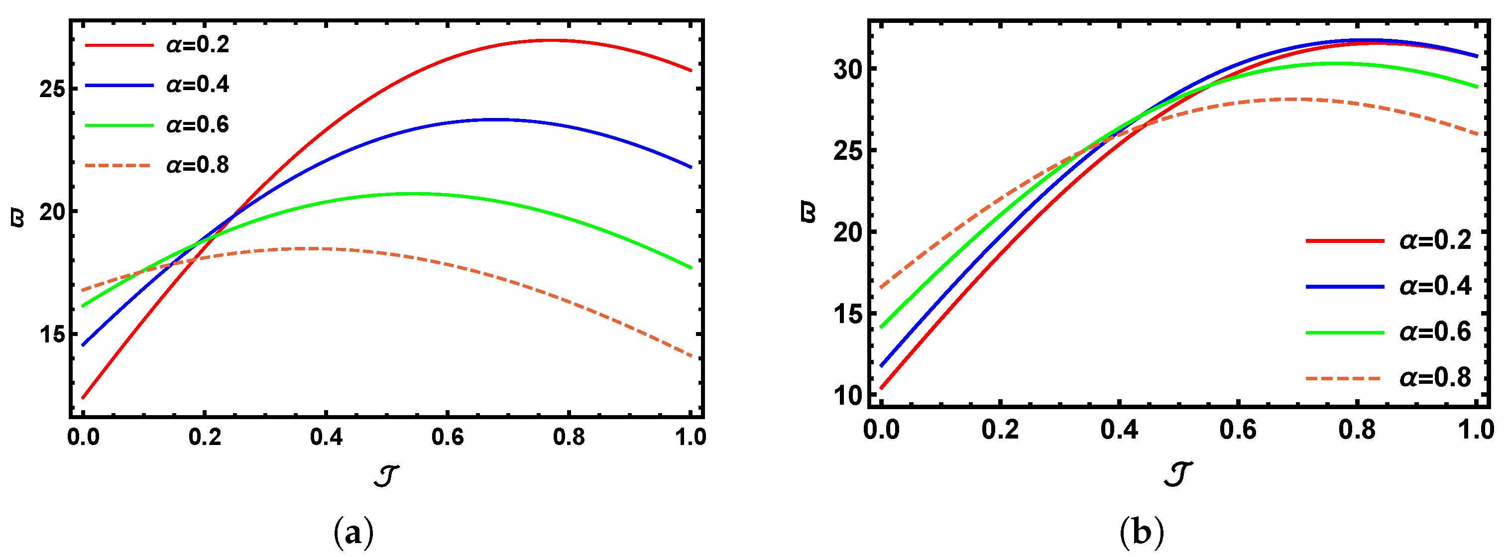
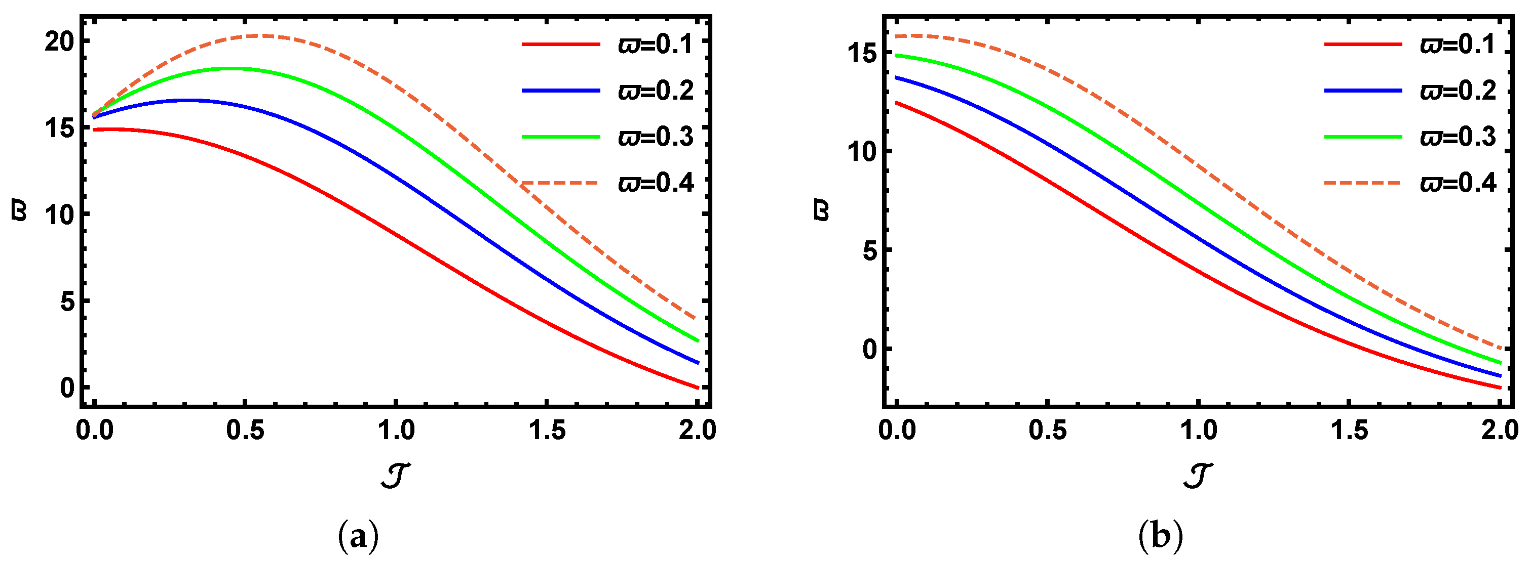
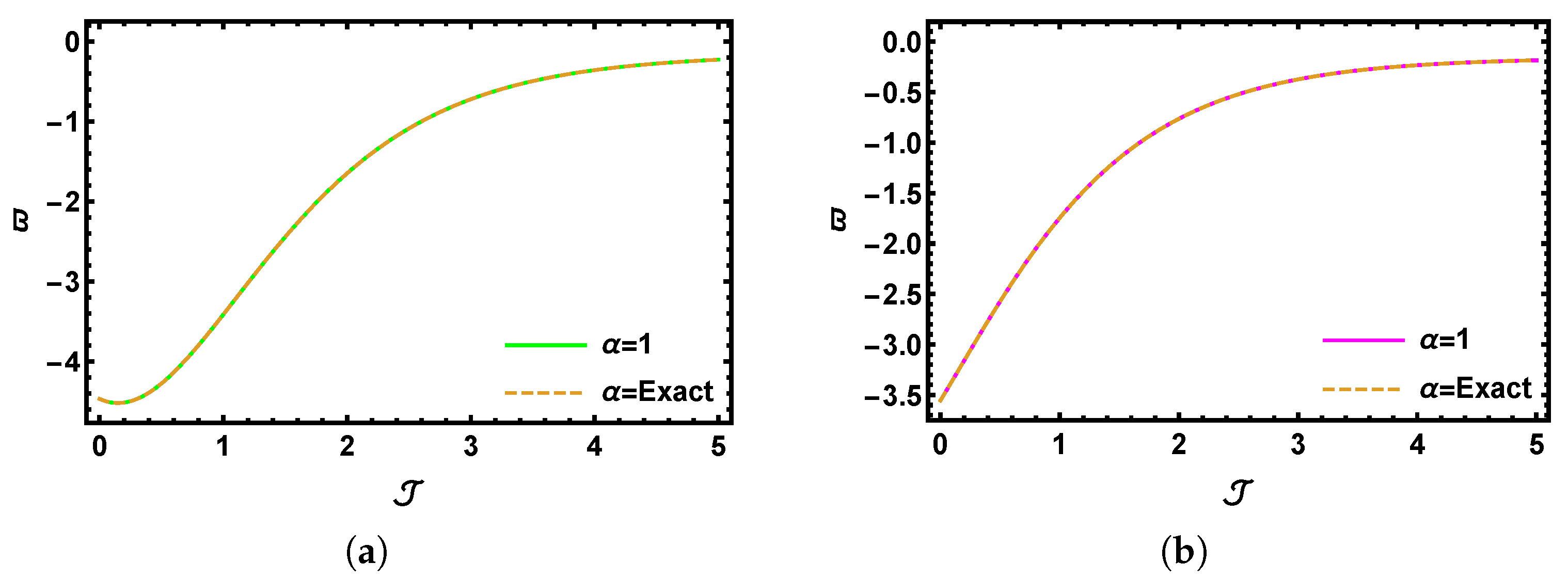
Figure 1a presents the 3D graphical representation generated from the numerical results of the SHTM for the time-fractional K-S model at α = 0.5 . In contrast, Figure 1b illustrates the corresponding physical behavior at α = 0.75 . Similarly, Figure 1c displays the output of the K-S problem at α = 1 , while Figure 1d captures the profile of the precise outcome within the domain 10 10 and 0 ϖ 0.1 for the K-S problem (Section 5.1). The graphical results demonstrate that as the fractional value of α increases, the outcome increasingly converges with the precise 3D model. Figure 2a,b provide a visual comparison of ϑ ( , ϖ ) over the interval 0 1 , showcasing the outcomes for ϖ = 0.2 (solid red line), α = 0.4 (solid blue line), α = 0.6 (solid green line), and α = 0.8 (dashed line). Figure 3a,b provide a visual comparison of ϑ ( , ϖ ) over the interval 0 2 , showcasing the outcomes for ϖ = 0.1 (solid red line), ϖ = 0.2 (solid blue line), ϖ = 0.3 (solid green line), and ϖ = 0.4 (dashed line) with α = 0.6 and α = 1 , respectively. Figure 4a illustrates the contrast between the SHTM findings and the exact outcomes over the interval 0 5 when α = 0.5 and ϖ = 0.5 , whereas Figure 4b offers the relationship across the SHTM and the precise outcomes over the interval 0 1 when α = 1 and ϖ = 0.1 . It is evident that the SHTM solution at α = 1 shows excellent accuracy to the precise outcomes that confirm the reliability of the proposed method. Moreover, the solution becomes increasingly precise as the fractional-order α value approaches unity.
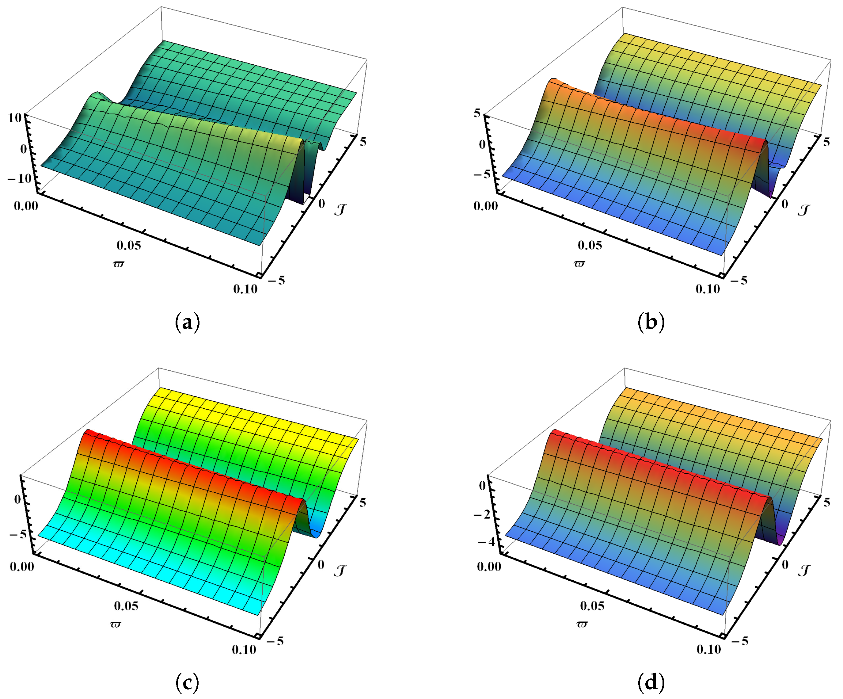
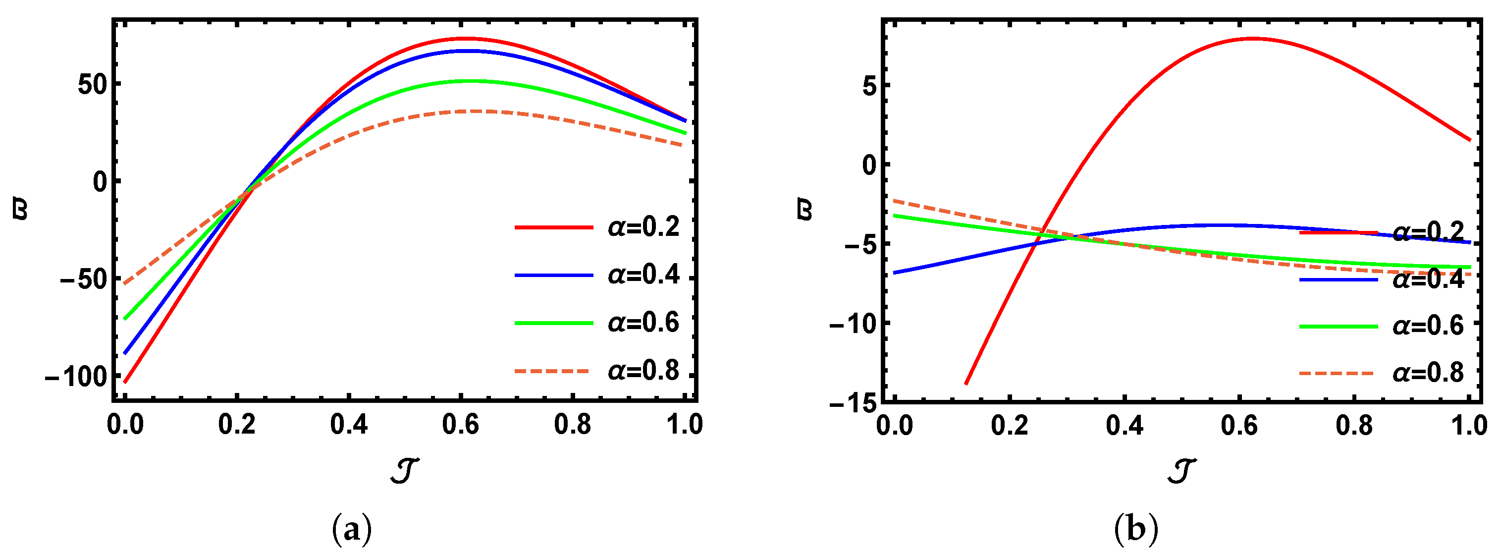
Figure 5a displays a three-dimensional visualization generated from the numerical results of the SHTM applied to the time fractional K-S model at α = 0.5 . Meanwhile, Figure 5b illustrates the corresponding physical structure for α = 0.75 . Figure 5c shows the graphical outcome of the K-S problem for the classical case when α = 1 . Lastly, Figure 5d presents the behavior of the precise outcomes for the time-fractional K-S problem within the limited domains 5 5 and 0 ϖ 0.1 , associated with the previously mentioned problem (Section 5.2). The graphical outcomes indicate that when the fractional value α is higher, the profile progressively aligns with the exact 3D solution. Figure 6a,b provide a visual comparison for ϑ ( , ϖ ) over the interval 0 1 , showcasing the outcomes for ϖ = 0.2 (solid red line), α = 0.4 (solid blue line), α = 0.6 (solid green line), and α = 0.8 (dashed line). Figure 7a,b provide a visual comparison of ϑ ( , ϖ ) over the interval 0 2 , showcasing the outcomes for ϖ = 0.1 (solid red line), ϖ = 0.2 (solid blue line), ϖ = 0.3 (solid green line), and ϖ = 0.4 (dashed line) with α = 0.6 and α = 1 , respectively. Figure 8a shows the comparison between the SHTM results with the precise results over the interval 0 5 when α = 0.5 and ϖ = 0.5 , whereas Figure 8b displays an analysis with the SHTM and the precise outcomes over the interval 0 5 when α = 1 and ϖ = 0.1 . The comparison clearly demonstrates that the SHTM solution at α = 1 closely matches the exact values, confirming the reliability of the method. Additionally, the SHTM output improves as the fractional-order α value increases.
The SHTM yields rapid convergence, producing results that closely match the exact solution after just a few iterations, particularly when α = 1 . Both the graphical representations and tabulated data confirm that the proposed method is not only accurate but also efficient and dependable for analyzing the time-fractional EM model.

7. Concluding Remarks

In the present study, we have investigated the fractional behavior of nonlinear time-fractional Kuramoto–Sivashinsky equations using an advanced numerical technique known as the Sumudu homotopy transform method. By employing the Caputo definition of fractional derivatives, we address the complexities of systems that cannot be effectively modeled with classical integer-order derivatives. Our methodology involves applying the Sumudu transform to convert the fractional components into a simpler form within the Sumudu space, which results in a nonlinear recurrence relation. We efficiently managed the nonlinear terms that arise during this process using He’s polynomials within the framework of the homotopy perturbation method.
Furthermore, two numerical applications were presented to validate the reliability and practicality of the approach. This method produced a convergent series solution through a recursive process that starts with the initial condition, without necessitating any assumptions or parameter constraints. Our findings show that this approach yields accurate results with fewer iterations and significantly reduced computational time compared to conventional methods.
Finally, we have included both 2D and 3D graphical visualizations of the results to clarify the numerical findings. These results confirm that our proposed approach is a robust, efficient, and reliable tool for solving a wide range of fractional-order linear and nonlinear problems. In the future, we aim to extend this method to more complex models involving time–space fractional derivatives in various scientific and engineering applications.

Author Contributions

Methodology, M.N.; Software, L.F.I.; Investigation, M.N.; Writing—original draft, M.N.; Writing—review & editing, L.F.I.; Funding acquisition, L.F.I. All authors have read and agreed to the published version of the manuscript.

Funding

The invoice was paid from the funds of the University of Oradea.

Data Availability Statement

The original contributions presented in this study are included in the article. Further inquiries can be directed to the corresponding authors.

Conflicts of Interest

The authors declare no conflicts of interest.

References

  1. Miller, K.S.; Ross, B. An Introduction to the Fractional Calculus and Fractional Differential Equations; Wiley: New York, NY, USA, 1993. [Google Scholar]
  2. Podlubny, I. Fractional Differential Equations; Academic Press: New York, NY, USA, 1999. [Google Scholar]
  3. Diethelm, K.; Ford, N.J. Analysis of fractional differential equations. J. Math. Anal. Appl. 2002, 265, 229–248. [Google Scholar] [CrossRef]
  4. Mainardi, F. Fractional calculus in wave propagation problems. Forum Berl. Math. Ges. 2012, 19, 20–52. [Google Scholar]
  5. Gomez-Aguilar, J.; Atangana, A. Applications of Fractional Calculus to Modeling in Dynamics and Chaos; CRC Press: Boca Raton, FL, USA, 2022. [Google Scholar]
  6. Ameen, I.G.; Baleanu, D.; Hussien, H.S. Efficient method for solving nonlinear weakly singular kernel fractional integro-differential equations. AIMS Math. 2024, 9, 15819–15836. [Google Scholar] [CrossRef]
  7. Ghader, G.; Reza, P.; Yavar, K.Y. Three-Dimensional and Multiple Image Encryption Algorithm Using a Fractional-Order Chaotic System. Computation 2025, 13, 115. [Google Scholar]
  8. Valério, D.; Machado, J.; Kiryakova, V. Some pioneers of the applications of fractional calculus. Fract. Calc. Appl. Anal. 2014, 17, 552–578. [Google Scholar] [CrossRef]
  9. Sun, H.; Zhang, Y.; Baleanu, D.; Chen, W.; Chen, Y. A new collection of real world applications of fractional calculus in science and engineering. Commun. Nonlinear Sci. Numer. Simul. 2018, 64, 213–231. [Google Scholar] [CrossRef]
  10. Magin, R.L. Fractional calculus models of complex dynamics in biological tissues. Comput. Math. Appl. 2010, 59, 1586–1593. [Google Scholar] [CrossRef]
  11. Kumar, S.; Yildirim, A.; Khan, Y.; Wei, L. A fractional model of the diffusion equation and its analytical solution using Laplace transform. Sci. Iran. 2012, 19, 1117–1123. [Google Scholar] [CrossRef]
  12. Huang, L.; Li, X.F.; Zhao, Y.; Duan, X.Y. Approximate solution of fractional integro-differential equations by Taylor expansion method. Comput. Math. Appl. 2011, 62, 1127–1134. [Google Scholar] [CrossRef]
  13. Nawaz, R.; Zada, L.; Ullah, F.; Ahmad, H.; Ayaz, M.; Ahmad, I.; Nofal, T.A. An extension of optimal auxiliary function method to fractional order high dimensional equations. Alex. Eng. J. 2021, 60, 4809–4818. [Google Scholar] [CrossRef]
  14. Ali, A.; Senu, N.; Wahi, N.; Almakayeel, N.; Ahmadian, A. An adaptive algorithm for numerically solving fractional partial differential equations using hermite wavelet artificial neural networks. Commun. Nonlinear Sci. Numer. Simul. 2024, 137, 108121. [Google Scholar] [CrossRef]
  15. Sartanpara, P.P.; Meher, R.; Meher, S. The generalized time-fractional Fornberg–Whitham equation: An analytic approach. Partial. Differ. Equ. Appl. Math. 2022, 5, 100350. [Google Scholar] [CrossRef]
  16. Sontakke, B.R.; Shelke, A.S.; Shaikh, A.S. Solution of non-linear fractional differential equations by variational iteration method and applications. Far East J. Math. Sci. 2019, 110, 113–129. [Google Scholar] [CrossRef]
  17. ur Rahman, M.; Arfan, M.; Shah, Z.; Alzahrani, E. Evolution of fractional mathematical model for drinking under Atangana-Baleanu Caputo derivatives. Phys. Scr. 2021, 96, 115203. [Google Scholar] [CrossRef]
  18. Luo, X.; Nadeem, M.; Asjad, M.I.; Abdo, M.S. A Computational Approach for the Calculation of Temperature Distribution in Casting-Mould Heterogeneous System with Fractional Order. Comput. Math. Methods Med. 2022, 2022, 3648277. [Google Scholar] [CrossRef]
  19. Nadeem, M.; Li, Z. A new strategy for the approximate solution of fourth-order parabolic partial differential equations with fractional derivative. Int. J. Numer. Methods Heat Fluid Flow 2022, 33, 1062–1075. [Google Scholar] [CrossRef]
  20. Liu, F.; Liu, J.; Nadeem, M. A numerical strategy for the approximate solution of the nonlinear time-fractional foam drainage equation. Fractal Fract. 2022, 6, 452. [Google Scholar] [CrossRef]
  21. Porshokouhi, M.G.; Ghanbari, B. Application of He’s variational iteration method for solution of the family of Kuramoto–Sivashinsky equations. J. King Saud Univ.-Sci. 2011, 23, 407–411. [Google Scholar] [CrossRef]
  22. Kilicman, A.; Silambarasan, R. Modified Kudryashov method to solve generalized Kuramoto-Sivashinsky equation. Symmetry 2018, 10, 527. [Google Scholar] [CrossRef]
  23. Grimshaw, R.; Hooper, A. The non-existence of a certain class of travelling wave solutions of the Kuramoto-Sivashinsky equation. Phys. D Nonlinear Phenom. 1991, 50, 231–238. [Google Scholar] [CrossRef]
  24. Liu, X. Gevrey class regularity and approximate inertial manifolds for the Kuramoto-Sivashinsky equation. Phys. D Nonlinear Phenom. 1991, 50, 135–151. [Google Scholar] [CrossRef]
  25. Veeresha, P.; Prakasha, D. Solution for fractional Kuramoto–Sivashinsky equation using novel computational technique. Int. J. Appl. Comput. Math. 2021, 7, 33. [Google Scholar] [CrossRef]
  26. Sahoo, S.; Ray, S.S. New approach to find exact solutions of time-fractional Kuramoto–Sivashinsky equation. Phys. A Stat. Mech. Its Appl. 2015, 434, 240–245. [Google Scholar] [CrossRef]
  27. Kumar, A. Dynamic behaviour and semi-analytical solution of nonlinear fractional-order Kuramoto–Sivashinsky equation. Pramana 2024, 98, 48. [Google Scholar] [CrossRef]
  28. Wang, J.; Jiang, X.; Yang, X.; Zhang, H. A new robust compact difference scheme on graded meshes for the time-fractional nonlinear Kuramoto–Sivashinsky equation. Comput. Appl. Math. 2024, 43, 381. [Google Scholar] [CrossRef]
  29. Shah, R.; Khan, H.; Baleanu, D.; Kumam, P.; Arif, M. A semi-analytical method to solve family of Kuramoto–Sivashinsky equations. J. Taibah Univ. Sci. 2020, 14, 402–411. [Google Scholar] [CrossRef]
  30. Kurulay, M.; Secer, A.; Akinlar, M.A. A new approximate analytical solution of Kuramoto-Sivashinsky equation using homotopy analysis method. Appl. Math. Inf. Sci. 2013, 7, 267–271. [Google Scholar] [CrossRef]
  31. Saad Alshehry, A.; Imran, M.; Khan, A.; Shah, R.; Weera, W. Fractional view analysis of Kuramoto–Sivashinsky equations with non-singular kernel operators. Symmetry 2022, 14, 1463. [Google Scholar] [CrossRef]
  32. Lakestani, M.; Dehghan, M. Numerical solutions of the generalized Kuramoto–Sivashinsky equation using B-spline functions. Appl. Math. Model. 2012, 36, 605–617. [Google Scholar] [CrossRef]
  33. Elbeleze, A.A.; Kılıçman, A.; Taib, B.M. Homotopy Perturbation Method for Fractional Black-Scholes European Option Pricing Equations Using Sumudu Transform. Math. Probl. Eng. 2013, 2013, 524852. [Google Scholar] [CrossRef]
  34. Hamed, S.H.; Yousif, E.A.; Arbab, A.I. Analytic and Approximate Solutions of the Space-Time Fractional Schrödinger Equations by Homotopy Perturbation Sumudu Transform Method. Abstr. Appl. Anal. 2014, 2014, 863015. [Google Scholar] [CrossRef]
  35. Alomari, A. Homotopy-Sumudu transforms for solving system of fractional partial differential equations. Adv. Differ. Equ. 2020, 2020, 222. [Google Scholar] [CrossRef]
  36. Sarikaya, M.Z.; Ogunmez, H. On New Inequalities via Riemann-Liouville Fractional Integration. Abstr. Appl. Anal. 2012, 2012, 428983. [Google Scholar] [CrossRef]
  37. Jarad, F.; Abdeljawad, T. A modified Laplace transform for certain generalized fractional operators. Results Nonlinear Anal. 2018, 1, 88–98. [Google Scholar]
  38. Katatbeh, Q.D.; Belgacem, F.B.M. Applications of the Sumudu transform to fractional differential equations. Nonlinear Stud. 2011, 18, 99–112. [Google Scholar]
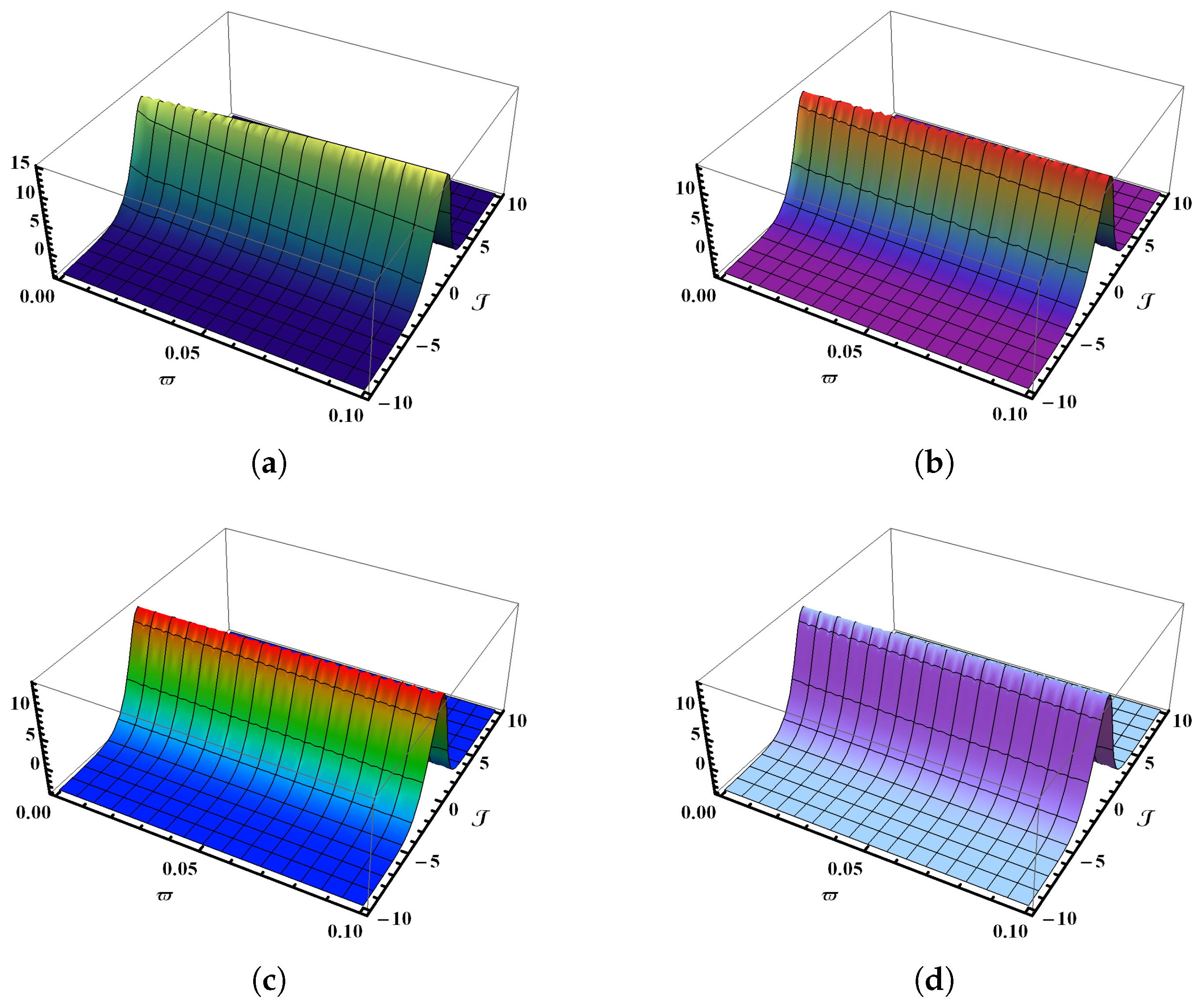
Figure 1. Comparison of 3D graphical renderings of SHTM results with exact results for ϑ ( , ϖ ) with multiple values of fractional-order α . (a) shows 3D graphics of SHTM results for ϑ ( , ϖ ) using α = 0.50 ; (b) shows 3D graphics of SHTM results for ϑ ( , ϖ ) using α = 0.75 ; (c) shows 3D graphics of SHTM results for ϑ ( , ϖ ) using α = 1 ; (d) shows 3D graphics of exact results for ϑ ( , ϖ ) .
Fractalfract 09 00418 g001
Figure 2. Graphs of 2D visual comparison between SHTM results and the precise outcomes for ϑ ( , ϖ ) with multiple fractional values of α when 0 1 with (a) ϖ = 0.5 and (b) ϖ = 1 .
Fractalfract 09 00418 g002
Figure 3. Graphs of 2D visual comparison between SHTM results and the precise outcomes for ϑ ( , ϖ ) with multiple values of ϖ when 0 2 with (a) α = 0.5 and (b) α = 1 .
Fractalfract 09 00418 g003
Figure 4. Results of 2D graphical comparison of SHTM results with precise outcomes with fractional values of α = 1 when 0 5 with (a) ϖ = 0.5 and (b) ϖ = 1 .
Fractalfract 09 00418 g004
Figure 5. Comparison of 3D graphical renderings of SHTM results with exact results for ϑ ( , ϖ ) with multiple values of fractional-order α . (a) shows 3D graphics of SHTM results for ϑ ( , ϖ ) using α = 0.50 ; (b) shows 3D graphics of SHTM results for ϑ ( , ϖ ) using α = 0.75 ; (c) shows 3D graphics of SHTM results for ϑ ( , ϖ ) using α = 1 ; (d) shows 3D graphics of exact results for ϑ ( , ϖ ) .
Fractalfract 09 00418 g005
Figure 6. A 2D visual comparison between SHTM results and the precise outcomes for ϑ ( , ϖ ) with multiple fractional values of α when 0 1 with (a) ϖ = 0.5 and (b) ϖ = 1 .
Fractalfract 09 00418 g006
Figure 7. A 2D visual comparison between SHTM results and the precise outcomes for ϑ ( , ϖ ) with multiple values of ϖ when 0 2 with (a) α = 0.5 and (b) α = 1 .
Fractalfract 09 00418 g007
Figure 8. A 2D graphical comparison of SHTM results with precise outcomes with fractional values of α = 1 when 0 5 with (a) ϖ = 0.5 and (b) ϖ = 1 .
Fractalfract 09 00418 g008
Disclaimer/Publisher’s Note: The statements, opinions and data contained in all publications are solely those of the individual author(s) and contributor(s) and not of MDPI and/or the editor(s). MDPI and/or the editor(s) disclaim responsibility for any injury to people or property resulting from any ideas, methods, instructions or products referred to in the content.