Parameterized Fractal–Fractional Analysis of Ostrowski- and Simpson-Type Inequalities with Applications

Abstract

In this paper, we first introduce a parametric identity for generalized differentiable functions using a generalized fractal–fractional integral operators. Based on this identity, we establish several variants of parameterized inequalities for functions whose local fractional derivatives in absolute value satisfy generalized convexity conditions. Furthermore, we demonstrate that our main results reduce to well-known Ostrowski- and Simpson-type inequalities by selecting suitable parameters. These inequalities contribute to finding tight bounds for various integrals over fractal spaces. By comparing the classical Hölder and Power mean inequalities with their new generalized versions, we show that the improved forms yield sharper and more refined upper bounds. In particular, we illustrate that the generalizations of Hölder and Power mean inequalities provide better results when applied to fractal integrals, with their tighter bounds supported by graphical representations. Finally, a series of applications are discussed, including generalized special means, generalized probability density functions and generalized quadrature formulas, which highlight the practical significance of the proposed results in fractal analysis.

1. Introduction and Preliminaries

Convexity is a very important concept in mathematical analysis and finds applications in such areas as optimization, economics and functional analysis. To say that a function is convex is to say that for any two points on its graph, the straight line segment joining them lies above or on the graph itself. This apparently obvious geometric property has a variety of powerful mathematical consequences. For example, convexity plays a fundamental role in the development of important inequalities and the construction of important approximation methods that play a vital role in many areas of mathematics and computation. Convexity can reveal crucial information about the behavior of complex functions, so that such functions and systems may be understood more effectively in terms of their properties. This makes convexity not only a geometric concept but also a tool that facilitates deeper analysis and clearer conclusions in both theoretical and applied contexts. It ranges from the effectiveness of optimization algorithms to helping economists model consumer behavior and is, therefore, an essential concept in modern mathematics and its applications.

Definition 1

([1]). Let a function $\mathsf{ϝ}:I\subseteq \mathbb{R}\to \mathbb{R},$ be called convex if

$$\begin{array}{c}\hfill \mathsf{ϝ}({\tau }_o{\sigma }_o+(1-{\tau }_o){\rho }_o)\le {\tau }_o\mathsf{ϝ}\left({\sigma }_o\right)+(1-{\tau }_o)\mathsf{ϝ}\left({\rho }_o\right),\end{array}$$

(1)

for each ${\sigma }_o,{\rho }_o\in I$ and ${\tau }_o\in [0,1]$ hold.

Theorem 1

([2]). Let a function $\mathsf{ϝ}:\mathrm{I}\to \mathbb{R},$ be convex. Then, the below mentioned inequality holds, famously known as the Hermite–Hadamard inequality:

$$\begin{array}{c}\hfill \mathsf{ϝ}\left(\frac{{\sigma }_o+{\rho }_o}{2}\right)\le \frac{1}{{\rho }_o-{\sigma }_o}{\int }_{{\sigma }_o}^{{\rho }_o}\mathsf{ϝ}\left(\varkappa \right)d\varkappa \le \frac{\mathsf{ϝ}\left({\sigma }_o\right)+\mathsf{ϝ}\left({\rho }_o\right)}{2},\end{array}$$

(2)

for all ${\sigma }_o,{\rho }_o\in I$ with ${\sigma }_o<{\rho }_o$.

Based on the double set of inequalities (2), several generalizations in terms of notable convexities and functional properties have been formulated; brief collections of them are artistically compiled in monographs [2,3].

The Ostrowski inequality approximates the deviation of the function’s values from the mean value of a smooth function within a defined interval. It gives an upper bound for an integral average $\frac{1}{{\rho }_o-{\sigma }_o}{\int }_{{\sigma }_o}^{{\rho }_o}\mathsf{ϝ}\left(\varkappa \right)d\varkappa$ for all $\varkappa \in [{\sigma }_o,{\rho }_o].$ This inequality is more pertinent to the theory of mathematical inequalities, as it provides an exact measure of how much the values of $\mathsf{ϝ}\left(\varkappa \right)$ (a function) deviate from its mean.

Theorem 2

([4]). Let $\mathsf{ϝ}:I\subseteq \mathbb{R}\to \mathbb{R},$ be a differential mapping on $I^{\circ }$, the interior of the interval I, such that I $\in L[{\sigma }_o,{\rho }_o]$ where ${\sigma }_o,{\rho }_o\in$ I with ${\rho }_o>{\sigma }_o.$ If $|{\mathsf{ϝ}}^{\prime }\left({\tau }_o\right)|\le M$ for all ${\tau }_o\in [{\sigma }_o,{\rho }_o]$, then the below inequality holds:

$$\begin{array}{cc}\hfill & |\mathsf{ϝ}\left({\tau }_o\right)-\frac{1}{{\rho }_o-{\sigma }_o}{\int }_{{\sigma }_o}^{{\rho }_o}\mathsf{ϝ}\left(\varkappa \right)d\varkappa |\le M({\rho }_o-{\sigma }_o)\left[\frac{1}{4}-\frac{{({\tau }_o-\frac{{\sigma }_o+{\rho }_o}{2})}^2}{{({\rho }_o-{\sigma }_o)}^2}\right].\hfill \end{array}$$

(3)

In approximation theory, convexity is the main tool used to assess and enhance numerical algorithms for definite integral computations. Such numerical methods approximate the area under a curve, that is the integral of a function, which cannot be obtained exactly in many cases. Probably one of the best known methods to this end is Simpson’s rule, which is especially appreciated for its simplicity and high accuracy when applied on smooth functions in closed intervals. Simpson’s rule approximates definite integral values fitting quadratic polynomials to segments of the function as opposed to the piecewise linear approximations used by simpler methods, which gives the approximation a finer accuracy, especially for smooth and continuous functions. Because straight-line approximations, such as those used in the midpoint rule and the trapezoidal rule, are relatively crude, Simpson’s rule is far more accurate due to the better fit of quadratic polynomials to curvatures of the function. Therefore, Simpson’s rule has become an excellent choice for many applications in numerical integration since it has a good balance between simplicity and accuracy. Therefore, the role that convexity assumes aids in verifying that approximations conducted using the method of Simpson’s rule hold very strong weight; therefore, it forms a cornerstone application within the area of numerical analysis.

Butt et al. [5,6] developed fractional versions of Newton- and Simpson-type inequalities via majorization and Jensen–Hermite–Hadamard–Mercer type inequalities for generalized strongly convex functions on fractal sets. Saleh et al. [7] established analysis of Newton-type inequalities in the biparameterized fractional setting. Dragomir et al. [8,9] investigated the remainder term in Simpson’s formula, while [10] introduced fractional Simpson’s inequalities for functions exhibiting absolute value convexity in their second derivatives. Butt et al. [11] established Milne-type inequalities for strongly multiplicative convex functions via multiplicative calculus. Li et al. [12] derived Hermite–Hadamard-type results for fractional calculus with exponential kernels. Butt et al. [13] introduced some novel approaches to Simpson-type estimates via fractal–fractional calculus for twice differentiable functions. For further studies on Newton-type inequalities see [14,15,16,17].

In many areas of mathematics, Simpson’s inequality is significant. For functions that are four times continuously differentiable, the classical Simpson’s inequality is written as follows:

Theorem 3

([18]). Let $\mathsf{ϝ}:[{\sigma }_o,{\rho }_o]\to \mathbb{R},$ is a four time continuously differentiable mapping on $({\sigma }_o,{\rho }_o)$ and let $\left|\right|{\mathsf{ϝ}}^{\left(4\right)}{\left|\right|}_{\infty }={sup}_{\varkappa \in ({\sigma }_o,{\rho }_o)}\left|{\mathsf{ϝ}}^{\left(4\right)}\left(\varkappa \right)\right|<\infty$ then the following inequality holds:

$$\begin{array}{cc}\hfill & |\frac{1}{3}\left[\frac{\mathsf{ϝ}\left({\sigma }_o\right)+\mathsf{ϝ}\left({\rho }_o\right)}{2}+2\mathsf{ϝ}\left(\frac{{\sigma }_o+{\rho }_o}{2}\right)\right]-\frac{1}{{\rho }_o-{\sigma }_o}{\int }_{{\sigma }_o}^{{\rho }_o}\mathsf{ϝ}\left(\varkappa \right)d\varkappa |\hfill \\ \hfill & \le \frac{1}{2880}\left|\right|{\mathsf{ϝ}}^{\left(4\right)}{\left|\right|}_{\infty }{({\rho }_o-{\sigma }_o)}^4.\hfill \end{array}$$

One of the most well-known and frequently applied techniques in this field is Simpson’s quadrature formulas. Interestingly, this mathematical tool is widely used to estimate the error related to quadrature formulas.

Theorem 4

([18]). Let $\mathsf{ϝ}:[{\sigma }_o,{\rho }_o]\to \mathbb{R},$ be a four-times continuously differentiable mapping on $({\sigma }_o,{\rho }_o)$ and let $\left|\right|{\mathsf{ϝ}}^{\left(4\right)}{\left|\right|}_{\infty }={sup}_{\varkappa \in ({\sigma }_o,{\rho }_o)}\left|{\mathsf{ϝ}}^{\left(4\right)}\left(\varkappa \right)\right|<\infty$, then the following inequality holds:

$$\begin{array}{cc}\hfill & |\frac{1}{8}\left[\mathsf{ϝ}\left({\sigma }_o\right)+3\mathsf{ϝ}\left(\frac{2{\sigma }_o+{\rho }_o}{3}\right)+3\mathsf{ϝ}\left(\frac{{\sigma }_o+2{\rho }_o}{3}\right)+\mathsf{ϝ}\left({\rho }_o\right)\right]-\frac{1}{{\rho }_o-{\sigma }_o}{\int }_{{\sigma }_o}^{{\rho }_o}\mathsf{ϝ}\left(\varkappa \right)d\varkappa |\hfill \\ \hfill & \le \frac{1}{6480}\left|\right|{\mathsf{ϝ}}^{\left(4\right)}{\left|\right|}_{\infty }{({\rho }_o-{\sigma }_o)}^4.\hfill \end{array}$$

For further work on Simpson’s inequality using different types of integral operators, we refer readers to [19,20,21].

Fractal sets are geometric structures known for their complexity, irregularity of shapes and their unique property of self-similarity. The same pattern occurs at different scales. The usual way of defining such structures is by means of recursive processes in which simple rules are iteratively applied to produce more complex shapes. Fractals are important in such fields as dynamical systems and signal processing because they are able to model natural phenomena displaying irregular patterns, i.e., the jagged edges of coastlines or the unpredictability of turbulent fluid flows. Other than their very direct applications, fractals have become important to mathematicians and scientists for quantifying complexity in any system or entity, as through the Hausdorff dimension, for instance, that would describe just how detailed or broken up a fractal was at different scales. This makes possible the catching of the detail involved in a fractal, thereby making its quantitative capture possible; in this sense, fractals serve as powerful tools in research, whether theoretical or applied.

For example, Butt et al. [22] introduced recent advances in fractal–fractional parametric inequalities and their applications. Akkurt et al. [23], Sarikaya and Budak et al. [24] and Tomar et al. [25] presented some generalized Ostrowski-type integral inequalities in terms of generalized moments, generalized convexity and generalized s-convexity, respectively. Erden and Sarikaya et al. [26] established some generalized Pompeiu-type inequalities and their corresponding applications within the framework of local fractional integrals. Atangana et al. in [27] introduced fractal–fractional derivatives and integrals, merging fractal and fractional calculus for predicting complex phenomena. Sun et al. in [28] developed some recent inequalities for generalized h-convex functions using local fractional operators with a Mittag–Leffler kernel. Waden et al., in [29], presented some observations on inequalities of local fractional integrals involving Mittag–Leffler kernels and (E,h)-convexity. Sun et al., in [30], established generalized Hermite–Hadamard inequalities via local fractional integrals for s-preinvex functions. Butt et al. [31] worked out the Hadamard–Mercer type inequalities along with their applications within the framework of fractal space. Recently, Atangana et al., in [32], introduced some application of fractal–fractional operators in modeling attractors of chaotic synamics. For additional results consistent with local fractional calculus, it is possible to refer to [33,34,35,36,37] and the bibliographies quoted within them. Additionally, some applications based on fractal space can be searched within the literature, for instance, in [38,39,40,41,42] and the bibliographies quoted within them.

We recall the Gao-Yang-Kang concept to explain the definition of the local fractional integral and local fractional derivative, keeping in mind the set ${\mathrm{R}}^{{\alpha }_o}$ of real line numbers. A recent development in fractional directions is the theory of Yang’s local fractional calculus, which can be given as follows:

• For $0<{\alpha }_o\le 1$, the ${\alpha }_o$-type set of the element are given below:
• ${\mathbb{Z}}^{{\alpha }_o}$: The ${\alpha }_o$-type set of integer numbers is used to define the set $\left\{0^{{\alpha }_o},\pm 1^{{\alpha }_o},\pm 2^{{\alpha }_o},\dots ,\pm n^{{\alpha }_o},\dots \right\}$.
• ${\mathbb{Q}}^{{\alpha }_o}$: The ${\alpha }_o$-type set of rational numbers is used to define the set
• &$\left\{{\mathfrak{m}}^{{\alpha }_o}={\left(\frac{\varkappa }{{\varkappa }_1}\right)}^{{\alpha }_o}:\varkappa ,{\varkappa }_1\in \mathbb{Z},{\varkappa }_1\ne 0\right\}$.
• ${\mathbb{J}}^{{\alpha }_o}$: The ${\alpha }_o$-type set of irrational numbers is used to define the set
• & $\left\{{\mathfrak{m}}^{{\alpha }_o}\ne {\left(\frac{\varkappa }{{\varkappa }_1}\right)}^{{\alpha }_o}:\varkappa ,{\varkappa }_1\in \mathbb{Z},{\varkappa }_1\ne 0\right\}$.
• ${\mathbb{R}}^{{\alpha }_o}$: The ${\alpha }_o$-type set of real numbers is used to define the set ${\mathbb{R}}^{{\alpha }_o}$=${\mathbb{Q}}^{{\alpha }_o}$∪${\mathbb{J}}^{{\alpha }_o}$.
• The following operations hold for ${\varkappa }^{{\alpha }_o},{{\varkappa }_1}^{{\alpha }_o},$ and ${{\tau }_o}^{{\alpha }_o},$ belong to the set ${\mathbb{R}}^{{\alpha }_o},$ of real line numbers:

(i)

${\varkappa }^{{\alpha }_o}+{{\varkappa }_1}^{{\alpha }_o}$ and ${\varkappa }^{{\alpha }_o}{{\varkappa }_1}^{{\alpha }_o}$ belong to the set ${\mathbb{R}}^{{\alpha }_o}$;

(ii)

${\varkappa }^{{\alpha }_o}+{{\varkappa }_1}^{{\alpha }_o}={{\varkappa }_1}^{{\alpha }_o}+{\varkappa }^{{\alpha }_o}={(\varkappa +{\varkappa }_1)}^{{\alpha }_o}={(\varkappa +{\varkappa }_1)}^{{\alpha }_o}$;

(iii)

${\varkappa }^{{\alpha }_o}+({{\varkappa }_1}^{{\alpha }_o}+{{{\tau }_o}_o}^{{\alpha }_o})={(\varkappa +{\varkappa }_1)}^{{\alpha }_o}+{{\tau }_o}^{{\alpha }_o}$;

(iv)

${\varkappa }^{{\alpha }_o}{{\varkappa }_1}^{{\alpha }_o}={{\varkappa }_1}^{{\alpha }_o}{\varkappa }^{{\alpha }_o}={\left(\varkappa {\varkappa }_1\right)}^{{\alpha }_o}={\left({\varkappa }_1\varkappa \right)}^{{\alpha }_o}$;

(v)

${\varkappa }^{{\alpha }_o}\left({{\varkappa }_1}^{{\alpha }_o}{{\tau }_o}^{{\alpha }_o}\right)=\left({\varkappa }^{{\alpha }_o}{{\varkappa }_1}^{{\alpha }_o}\right){{\tau }_o}^{{\alpha }_o}$;

(vi)

${\varkappa }^{{\alpha }_o}({{\varkappa }_1}^{{\alpha }_o}+{{\tau }_o}^{{\alpha }_o})={\varkappa }^{{\alpha }_o}{{\varkappa }_1}^{{\alpha }_o}+{\varkappa }^{{\alpha }_o}{{\tau }_o}^{{\alpha }_o}$;

(vii)

${\varkappa }^{{\alpha }_o}+0^{{\alpha }_o}=0^{{\alpha }_o}+{\varkappa }^{{\alpha }_o}={\varkappa }^{{\alpha }_o}$ and ${\varkappa }^{{\alpha }_o}{1}^{{\alpha }_o}=1^{{\alpha }_o}{\varkappa }^{{\alpha }_o}={\varkappa }^{{\alpha }_o}$;

(viii)

${\varkappa }^{{\alpha }_o}={{\varkappa }_1}^{{\alpha }_o}$ when and only when $\varkappa ={\varkappa }_1,\varkappa ,{\varkappa }_1\subset \mathbb{R}$;

(ix)

${\varkappa }^{{\alpha }_o}\ge {\varkappa }_1$ when and only when $\varkappa \ge {\varkappa }_1,\varkappa ,{\varkappa }_1\subset \mathbb{R}$;

(x)

${\left({\varkappa }^{{\alpha }_o}\right)}^{{\mathrm{q}}_{\mathrm{o}}}$=${\left({\varkappa }^{{\mathrm{q}}_{\mathrm{o}}}\right)}^{{\alpha }_o},{\mathrm{q}}_{\mathrm{o}}>0$ and $\varkappa >0$.

Definition 2

([42]). For any ${\sigma }_o,{\rho }_o\in \mathrm{I}$ and ${\tau }_o\in [0,1]$, if the following inequality

$$\begin{array}{c}\hfill \mathsf{ϝ}({\tau }_o{\sigma }_o+(1-{\tau }_o){\rho }_o)\le {{\tau }_o}^{{\alpha }_o}\mathsf{ϝ}\left({\sigma }_o\right)+{(1-{\tau }_o)}^{{\alpha }_o}\mathsf{ϝ}\left({\rho }_o\right),\end{array}$$

holds, then ϝ is called the generalized convex function on I, where ϝ:$I\subseteq \mathbb{R}$ $\to {\mathbb{R}}^{{\alpha }_o}.$

Theorem 5

([31]). If $\mathsf{ϝ}\left(\varkappa \right)\in {}_{{\sigma }_o}I_{{\rho }_o}^{{\alpha }_o}$ is a generalized convex function on $[{\sigma }_o,{\rho }_o]$ with ${\sigma }_o<{\rho }_o$, then

$$\begin{array}{cc}\hfill \mathsf{ϝ}\left(\frac{{\sigma }_o+{\rho }_o}{2}\right)& \le \frac{\mathrm{\Gamma }\left(1+{\alpha }_o\right)}{{({\rho }_o-{\sigma }_o)}^{{\alpha }_o}}{}_{{\sigma }_o}I_{{\rho }_o}^{{\alpha }_o}\mathsf{ϝ}\left(\varkappa \right)\le \frac{\mathsf{ϝ}\left({\sigma }_o\right)+\mathsf{ϝ}\left({\rho }_o\right)}{2^{{\alpha }_o}}.\hfill \end{array}$$

In the recent past, Du et al., in [43], introduced the concept of generalized fractal fractional integral operators, as given below:

Definition 3

([44]). Let us consider a function $\eta :[0,\infty )\to [0^{{\alpha }_o},{\infty }^{{\alpha }_o})$ satisfying the following conditions:

$$\begin{array}{cc}\hfill & \frac{1}{\mathrm{\Gamma }(1+{\alpha }_o)}{\int }_0^1\frac{\eta \left({\tau }_o\right)}{{{\tau }_o}^{{\alpha }_o}}{\left(d{\tau }_o\right)}^{{\alpha }_o}<{\infty }^{{\alpha }_o}.\hfill \end{array}$$

The following right-sided and left-sided generalized fractal integral operators are, respectively,

$$\begin{array}{cc}\hfill & {}_{{{\sigma }_o}^{+}}\mathrm{I}_{\eta }^{{\alpha }_o}\mathsf{ϝ}\left(\varkappa \right)=\frac{1}{\mathrm{\Gamma }(1+{\alpha }_o)}{\int }_{{\sigma }_o}^{\varkappa }\frac{\eta (\varkappa -{\tau }_o)}{{(\varkappa -{\tau }_o)}^{{\alpha }_o}}\mathsf{ϝ}\left({\tau }_o\right){\left(d{\tau }_o\right)}^{{\alpha }_o},\hfill \end{array}$$

and

$$\begin{array}{cc}\hfill & {}_{{{\rho }_o}^{-}}\mathrm{I}_{\eta }^{{\alpha }_o}\mathsf{ϝ}\left(\varkappa \right)=\frac{1}{\mathrm{\Gamma }(1+{\alpha }_o)}{\int }_{\varkappa }^{{\rho }_o}\frac{\eta ({\tau }_o-\varkappa )}{{({\tau }_o-\varkappa )}^{{\alpha }_o}}\mathsf{ϝ}\left({\tau }_o\right){\left(d{\tau }_o\right)}^{{\alpha }_o}.\hfill \end{array}$$

Definition 4

([42]). Let a function that is not differentiable $\mathsf{ϝ}:\mathbb{R}\to {\mathbb{R}}^{{\alpha }_o},{\varkappa }_1\to \mathsf{ϝ}\left({\varkappa }_1\right)$ be called to be the local fractional continuous at ${\varkappa }_0$ if for any $\epsilon \in {\mathbb{R}}^{+}$ there exist $\delta \in {\mathbb{R}}^{+}$ such that

$$\begin{array}{c}\hfill |\mathsf{ϝ}\left({\varkappa }_1\right)-\mathsf{ϝ}\left({\varkappa }_0\right)|<{\epsilon }^{{\alpha }_o},\end{array}$$

(4)

holds for $|{\varkappa }_1-{\varkappa }_o|<\delta where\mathsf{ϝ},\delta \in \mathbb{R}.$ If $\mathrm{I}\left({\varkappa }_1\right)$ is local fractional that is continuous on the interval $({\sigma }_o,{\rho }_o)$, we denote $\mathsf{ϝ}\left(\varkappa \right)\in C_{{\alpha }_o}({\sigma }_o,{\rho }_o).$

Definition 5

([42]). The local fractional derivative of $\mathsf{ϝ}\left(\varkappa \right)$ of order ${\alpha }_o$ at $\varkappa ={\varkappa }_0$ is defined by

$$\begin{array}{c}\hfill {\mathsf{ϝ}}^{\left({\alpha }_o\right)}\left({\varkappa }_o\right)={\varkappa }_o{D}_{\varkappa }^{{\alpha }_o}\mathsf{ϝ}\left(\varkappa \right)=\frac{d^{\left({\alpha }_o\right)}\mathsf{ϝ}\left(\varkappa \right)}{d\left({\varkappa }^{{\alpha }_o}\right)}{|}_{\varkappa ={\varkappa }_o}=li{m}_{\varkappa \to {\varkappa }_o}\frac{{\Delta }^{{\alpha }_o}(\mathsf{ϝ}\left(\varkappa \right)-\mathsf{ϝ}\left({\varkappa }_o\right))}{{(\varkappa -{\varkappa }_o)}^{{\alpha }_o}},\end{array}$$

(5)

where ${\Delta }^{{\alpha }_o}(\mathsf{ϝ}\left(\varkappa \right)-\mathsf{ϝ}\left({\varkappa }_o\right))\cong \mathrm{\Gamma }(1+{\sigma }_o)(\mathsf{ϝ}\left(\varkappa \right)-\mathsf{ϝ}\left({\varkappa }_o\right))$ and $\mathrm{\Gamma }$ is the well-known gamma function. Let ${\mathsf{ϝ}}^{\left({\alpha }_o\right)}\left(\varkappa \right)=D_{\varkappa }^{{\alpha }_o}\mathsf{ϝ}\left(\varkappa \right)$. If there holds ${\mathsf{ϝ}}^{(\mathrm{k}+1){\alpha }_o}\left(\varkappa \right)$=$\stackrel{(\mathrm{k}+1)times}{\overbrace{D_{\varkappa }^{{\alpha }_o}\dots D_{\varkappa }^{{\alpha }_o}\mathsf{ϝ}\left(\varkappa \right)}}$ for any $\varkappa \in I\subseteq \mathbb{R}$, then we denote $\mathsf{ϝ}\in D_{(\mathrm{k}+1){\alpha }_o}\left(I\right)$, where $\mathrm{k}=0,1,2,3,\dots$

Definition 6

([42]). The local fractional integral of ϝ on the interval $[{\sigma }_o,{\rho }_o]$ of order ${\alpha }_o$ is defined by

$${}_{{\sigma }_o}\mathrm{I}_{{\rho }_o}^{\left({\alpha }_o\right)}=\frac{1}{\mathrm{\Gamma }({\alpha }_o+1)}{\int }_{{\sigma }_o}^{{\rho }_o}\mathsf{ϝ}\left(\varkappa \right){\left(d\varkappa \right)}^{{\alpha }_o}:=\frac{1}{\mathrm{\Gamma }({\alpha }_o+1)}\underset{\Delta \eta \to 0}{\lim }{{\Sigma }_o}_{j=0}^{\mathrm{N}-1}\mathsf{ϝ}\left({\eta }_{\mathrm{j}}\right){(\Delta {\eta }_{\mathrm{j}})}^{{\alpha }_o}$$

(6)

provided that the limit exists.

Here, it follows that ${}_{{\sigma }_o}\mathrm{I}_{{\rho }_o}^{\left({\alpha }_o\right)}\mathsf{ϝ}=0$ if ${\sigma }_o={\rho }_o$ and ${}_{{\sigma }_o}\mathrm{I}_{{\rho }_o}^{\left({\alpha }_o\right)}\mathsf{ϝ}={-}_{{\rho }_o}{\mathrm{I}}_{{\sigma }_o}^{\left({\alpha }_o\right)}\mathsf{ϝ},$ if ${\sigma }_o<{\rho }_o$.

Lemma 1.

We recall some important properties of the local fractional calculus (see [42]) that are necessary for our key conclusions.

The below mentioned properties are

(1) 

(The local fractional derivative of ${\varkappa }^{{\tau }_o{\alpha }_o}$ at the local level):

$$\begin{array}{c}\hfill \frac{d^{{\alpha }_o}{\varkappa }^{{\tau }_o{\alpha }_o}}{d{\varkappa }^{{\alpha }_o}}=\frac{\mathrm{\Gamma }(1+{\tau }_o{\alpha }_o)}{\mathrm{\Gamma }(1+({\tau }_o-1){\alpha }_o)}{\varkappa }^{({\tau }_o-1){\alpha }_o}.\end{array}$$

(2) 

(The local fractional integration is anti-differentiation):

Let $\mathsf{ϝ}\left(\varkappa \right)={{\mathsf{ϝ}}_o}^{\left({\alpha }_o\right)}\left(\varkappa \right)\in C_{{\alpha }_o}[{\sigma }_o,{\rho }_o]$. Then, we have

$$\begin{array}{c}\hfill {}_{{\sigma }_o}\mathrm{I}_{{\rho }_o}^{\left({\alpha }_o\right)}\mathsf{ϝ}\left(\varkappa \right)={\mathsf{ϝ}}_o\left({\rho }_o\right)-{\mathsf{ϝ}}_o\left({\sigma }_o\right).\end{array}$$

(3) 

(Local fractional integral by parts at a local level):

Let $\mathsf{ϝ}\left(\varkappa \right),{\mathsf{ϝ}}_o\left(\varkappa \right)\in D_{{\alpha }_o}[{\sigma }_o,{\rho }_o]$ and ${\mathsf{ϝ}}^{\left({\alpha }_o\right)}\left(\varkappa \right),{{\mathsf{ϝ}}_o}^{\left({\alpha }_o\right)}\left(\varkappa \right)\in C_{{\alpha }_o}[{\sigma }_o,{\rho }_o]$. Then, we have

$$\begin{array}{c}\hfill {}_{{\sigma }_o}\mathrm{I}_{{\rho }_o}^{\left({\alpha }_o\right)}\mathsf{ϝ}\left(\varkappa \right){{\mathsf{ϝ}}_o}^{\left({\alpha }_o\right)}\left(\varkappa \right)=\mathsf{ϝ}\left(\varkappa \right){\mathsf{ϝ}}_o{\left(\varkappa \right)|}_{{\sigma }_o}^{{\rho }_o}-{}_{{\sigma }_o}\mathrm{I}_{{\rho }_o}^{\left({\alpha }_o\right)}{\mathsf{ϝ}}^{\left({\alpha }_o\right)}\left(\varkappa \right){\mathsf{ϝ}}_o\left(\varkappa \right).\end{array}$$

Lemma 2.

The definite local fractional integrals of ${\varkappa }^{{\tau }_o{\alpha }_o}$ are as defined below:

$$\begin{array}{c}\hfill \frac{1}{\mathrm{\Gamma }(1+{\alpha }_o)}{\int }_{{\sigma }_o}^{{\rho }_o}{\varkappa }^{{\tau }_o{\alpha }_o}{\left(d\varkappa \right)}^{{\alpha }_o}=\frac{\mathrm{\Gamma }(1+{\tau }_o{\alpha }_o)}{\mathrm{\Gamma }(1+({\tau }_o+1){\alpha }_o)}({{\rho }_o}^{({\tau }_o+1){\alpha }_o}-{{\sigma }_o}^{({\tau }_o+1){\alpha }_o}),{\tau }_o\in \mathbb{R}.\end{array}$$

Recently, the well-known Hölder’s integral inequality on fractional sets, also referred to as the generalized Hölder’s integral inequality, has gained significant attention from researchers. This version was proposed by Yang, as noted below.

Lemma 3

([42]). Let the functions ϝ and ${\mathsf{ϝ}}_1$ be designated on the real-value interval $[{\sigma }_o,{\rho }_o]$ satisfying that $\mathsf{ϝ},{\mathsf{ϝ}}_1\in C_{{\alpha }_o}[{\sigma }_o,{\rho }_o]$, and also ${|\mathsf{ϝ}|}^{{\mathrm{p}}_{\mathrm{o}}}$ and $|{\mathsf{ϝ}}_1{|}^{{\mathrm{q}}_{\mathrm{o}}}$ be designated on the real-value interval $[{\sigma }_o,{\rho }_o]$ and both be local fractional integrals, ${\mathrm{p}}_{\mathrm{o}},{\mathrm{q}}_{\mathrm{o}}>1$, along with $\frac{1}{{\mathrm{p}}_{\mathrm{o}}}+\frac{1}{{\mathrm{q}}_{\mathrm{o}}}=1$. Then, the below mentioned set of integral inequalities hold:

$$\begin{array}{cc}\hfill & \frac{1}{\mathrm{\Gamma }(1+{\sigma }_o)}{\int }_{{\sigma }_o}^{{\rho }_o}|\mathsf{ϝ}\left(\varkappa \right){\mathsf{ϝ}}_1\left(\varkappa \right)|{\left(d\varkappa \right)}^{{\alpha }_o}\hfill \\ \hfill & \le {\left(\frac{1}{\mathrm{\Gamma }(1+{\alpha }_o)}{\int }_{{\sigma }_o}^{{\rho }_o}{|\mathsf{ϝ}\left(\varkappa \right)|}^{{\mathrm{p}}_{\mathrm{o}}}{\left(d\varkappa \right)}^{{\alpha }_o}\right)}^{\frac{1}{{\mathrm{p}}_{\mathrm{o}}}}{\left(\frac{1}{\mathrm{\Gamma }(1+{\alpha }_o)}{\int }_{{\sigma }_o}^{{\rho }_o}|{\mathsf{ϝ}}_1{\left(\varkappa \right)|}^{{\mathrm{q}}_{\mathrm{o}}}{\left(d\varkappa \right)}^{{\alpha }_o}\right)}^{\frac{1}{{\mathrm{q}}_{\mathrm{o}}}}.\hfill \end{array}$$

In 2021, Luo et al. proposed a modified version of Hölder’s integral inequality on fractal space, providing a tighter upper bound compared to the generalized Hölder’s integral inequality, as stated below.

Lemma 4

([45]). Let the functions ϝ and ${\mathsf{ϝ}}_1$ be designated on the real-value interval $[{\sigma }_o,{\rho }_o]$ satisfying that $\mathsf{ϝ},{\mathsf{ϝ}}_1\in C_{{\alpha }_o}[{\sigma }_o,{\rho }_o]$ and also the functions ${|\mathsf{ϝ}|}^{{\mathrm{p}}_{\mathrm{o}}}$ and $|{\mathsf{ϝ}}_1{|}^{{\mathrm{q}}_{\mathrm{o}}}$ be designated on the real-value interval $[{\sigma }_o,{\rho }_o]$ and both be local fractional integrals, ${\mathrm{p}}_{\mathrm{o}},{\mathrm{q}}_{\mathrm{o}}>1$ along with $\frac{1}{{\mathrm{p}}_{\mathrm{o}}}+\frac{1}{{\mathrm{q}}_{\mathrm{o}}}=1$. Then, the below-mentioned set of integral inequalities holds:

$$\begin{array}{cc}\hfill & \frac{1}{\mathrm{\Gamma }(1+{\sigma }_o)}{\int }_{{\sigma }_o}^{{\rho }_o}|\mathsf{ϝ}\left(\varkappa \right){\mathsf{ϝ}}_1\left(\varkappa \right)|{\left(d\varkappa \right)}^{{\alpha }_o}\hfill \\ \hfill & \le {\left(\frac{1}{{\rho }_o-{\sigma }_o}\right)}^{{\alpha }_o}\{{\left(\frac{1}{\mathrm{\Gamma }(1+{\alpha }_o)}{\int }_{{\sigma }_o}^{{\rho }_o}{({\rho }_o-\varkappa )}^{{\alpha }_o}{|\mathsf{ϝ}\left(\varkappa \right)|}^{{\mathrm{p}}_{\mathrm{o}}}{\left(d\varkappa \right)}^{{\alpha }_o}\right)}^{\frac{1}{{\mathrm{p}}_{\mathrm{o}}}}\hfill \\ \hfill & \times {\left(\frac{1}{\mathrm{\Gamma }(1+{\alpha }_o)}{\int }_{{\sigma }_o}^{{\rho }_o}{({\rho }_o-\varkappa )}^{{\alpha }_o}|{\mathsf{ϝ}}_1{\left(\varkappa \right)|}^{{\mathrm{q}}_{\mathrm{o}}}{\left(d\varkappa \right)}^{{\alpha }_o}\right)}^{\frac{1}{{\mathrm{q}}_{\mathrm{o}}}}\hfill \\ \hfill & +{\left(\frac{1}{\mathrm{\Gamma }(1+{\alpha }_o)}{\int }_{{\sigma }_o}^{{\rho }_o}{(\varkappa -{\sigma }_o)}^{{\alpha }_o}{|\mathsf{ϝ}\left(\varkappa \right)|}^{{\mathrm{p}}_{\mathrm{o}}}{\left(d\varkappa \right)}^{{\alpha }_o}\right)}^{\frac{1}{{\mathrm{p}}_{\mathrm{o}}}}\hfill \\ \hfill & \times {\left(\frac{1}{\mathrm{\Gamma }(1+{\alpha }_o)}{\int }_{{\sigma }_o}^{{\rho }_o}{(\varkappa -{\sigma }_o)}^{{\alpha }_o}|{\mathsf{ϝ}}_1{\left(\varkappa \right)|}^{{\mathrm{q}}_{\mathrm{o}}}{\left(d\varkappa \right)}^{{\alpha }_o}\right)}^{\frac{1}{{\mathrm{q}}_{\mathrm{o}}}}\}\hfill \\ \hfill & \le {\left(\frac{1}{\mathrm{\Gamma }(1+{\alpha }_o)}{\int }_{{\sigma }_o}^{{\rho }_o}{|\mathsf{ϝ}\left(\varkappa \right)|}^{{\mathrm{p}}_{\mathrm{o}}}{\left(d\varkappa \right)}^{{\alpha }_o}\right)}^{\frac{1}{{\mathrm{p}}_{\mathrm{o}}}}{\left(\frac{1}{\mathrm{\Gamma }(1+{\alpha }_o)}{\int }_{{\sigma }_o}^{{\rho }_o}|{\mathsf{ϝ}}_1{\left(\varkappa \right)|}^{{\mathrm{q}}_{\mathrm{o}}}{\left(d\varkappa \right)}^{{\alpha }_o}\right)}^{\frac{1}{{\mathrm{q}}_{\mathrm{o}}}}.\hfill \end{array}$$

In 2022, Yu et al. [46] provided a simple proof of the generalized power-mean integral inequality and introduced a modified version of it in the fractal setting, as stated below.

Lemma 5

([46]). For ${\mathrm{q}}_{\mathrm{o}}\ge 1,$ the functions ϝ and ${\mathsf{ϝ}}_1$ are designated on the real-value interval $[{\sigma }_o,{\rho }_o]$, satisfying that $\mathsf{ϝ},{\mathsf{ϝ}}_1\in C_{{\alpha }_o}[{\sigma }_o,{\rho }_o]$ and also the functions $|\mathsf{ϝ}|$ and $|\mathsf{ϝ}||{\mathsf{ϝ}}_1{|}^{{\mathrm{q}}_{\mathrm{o}}}$ are designated on the real-value interval $[{\sigma }_o,{\rho }_o]$ and both are local fractional integrals, then the below mentioned set of generalized power-mean integral inequalities holds:

$$\begin{array}{cc}\hfill & \frac{1}{\mathrm{\Gamma }(1+{\alpha }_o)}{\int }_{{\sigma }_o}^{{\rho }_o}|\mathsf{ϝ}\left(\varkappa \right){\mathsf{ϝ}}_1\left(\varkappa \right)|{\left(d\varkappa \right)}^{{\alpha }_o}\hfill \\ \hfill & \le {\left(\frac{1}{\mathrm{\Gamma }(1+{\alpha }_o)}{\int }_{{\sigma }_o}^{{\rho }_o}|\mathsf{ϝ}(\varkappa \left)\right|{\left(d\varkappa \right)}^{{\alpha }_o}\right)}^{1-\frac{1}{{\mathrm{q}}_{\mathrm{o}}}}{\left(\frac{1}{\mathrm{\Gamma }(1+{\alpha }_o)}{\int }_{{\sigma }_o}^{{\rho }_o}|\mathsf{ϝ}\left(\varkappa \right)||{\mathsf{ϝ}}_1{\left(\varkappa \right)|}^{{\mathrm{q}}_{\mathrm{o}}}{\left(d\varkappa \right)}^{{\alpha }_o}\right)}^{\frac{1}{{\mathrm{q}}_{\mathrm{o}}}}.\hfill \end{array}$$

Lemma 6

([46]). For ${\mathrm{q}}_{\mathrm{o}}\ge 1,$ the functions ϝ and ${\mathsf{ϝ}}_1$ are designated on the real-value interval $[{\sigma }_o,{\rho }_o]$, satisfying that $\mathsf{ϝ},{\mathsf{ϝ}}_1\in C_{{\alpha }_o}[{\sigma }_o,{\rho }_o]$ and also the functions $|\mathsf{ϝ}|$ and $|\mathsf{ϝ}||{\mathsf{ϝ}}_1{|}^{{\mathrm{q}}_{\mathrm{o}}}$ are designated on the real-value interval $[{\sigma }_o,{\rho }_o]$ and are both local fractional integrals, then the below-mentioned set of generalized improved power-mean integral inequalities holds:

$$\begin{array}{cc}\hfill & \frac{1}{\mathrm{\Gamma }(1+{\alpha }_o)}{\int }_{{\sigma }_o}^{{\rho }_o}|\mathsf{ϝ}\left(\varkappa \right){\mathsf{ϝ}}_1\left(\varkappa \right)|{\left(d\varkappa \right)}^{{\alpha }_o}\hfill \\ \hfill & \le {\left(\frac{1}{{\rho }_o-{\sigma }_o}\right)}^{{\alpha }_o}\{{\left(\frac{1}{\mathrm{\Gamma }(1+{\alpha }_o)}{\int }_{{\sigma }_o}^{{\rho }_o}{({\rho }_o-\varkappa )}^{{\alpha }_o}|\mathsf{ϝ}(\varkappa \left)\right|{\left(d\varkappa \right)}^{{\alpha }_o}\right)}^{1-\frac{1}{{\mathrm{q}}_{\mathrm{o}}}}\hfill \\ \hfill & \times {\left(\frac{1}{\mathrm{\Gamma }(1+{\alpha }_o)}{\int }_{{\sigma }_o}^{{\rho }_o}{({\rho }_o-\varkappa )}^{{\alpha }_o}|\mathsf{ϝ}\left(\varkappa \right)||{\mathsf{ϝ}}_1{\left(\varkappa \right)|}^{{\mathrm{q}}_{\mathrm{o}}}{\left(d\varkappa \right)}^{{\alpha }_o}\right)}^{\frac{1}{{\mathrm{q}}_{\mathrm{o}}}}\hfill \\ \hfill & +{\left(\frac{1}{\mathrm{\Gamma }(1+{\alpha }_o)}{\int }_{{\sigma }_o}^{{\rho }_o}{(\varkappa -{\sigma }_o)}^{{\alpha }_o}|\mathsf{ϝ}(\varkappa \left)\right|{\left(d\varkappa \right)}^{{\alpha }_o}\right)}^{1-\frac{1}{{\mathrm{q}}_{\mathrm{o}}}}\hfill \\ \hfill & \times {\left(\frac{1}{\mathrm{\Gamma }(1+{\alpha }_o)}{\int }_{{\sigma }_o}^{{\rho }_o}{(\varkappa -{\sigma }_o)}^{{\alpha }_o}|\mathsf{ϝ}\left(\varkappa \right)||{\mathsf{ϝ}}_1{\left(\varkappa \right)|}^{{\mathrm{q}}_{\mathrm{o}}}{\left(d\varkappa \right)}^{{\alpha }_o}\right)}^{\frac{1}{{\mathrm{q}}_{\mathrm{o}}}}\}\hfill \\ \hfill & \le {\left(\frac{1}{\mathrm{\Gamma }(1+{\alpha }_o)}{\int }_{{\sigma }_o}^{{\rho }_o}|\mathsf{ϝ}(\varkappa \left)\right|{\left(d\varkappa \right)}^{{\alpha }_o}\right)}^{1-\frac{1}{{\mathrm{q}}_{\mathrm{o}}}}{\left(\frac{1}{\mathrm{\Gamma }(1+{\alpha }_o)}{\int }_{{\sigma }_o}^{{\rho }_o}|\mathsf{ϝ}\left(\varkappa \right)||{\mathsf{ϝ}}_1{\left(\varkappa \right)|}^{{\mathrm{q}}_{\mathrm{o}}}{\left(d\varkappa \right)}^{{\alpha }_o}\right)}^{\frac{1}{{\mathrm{q}}_{\mathrm{o}}}}.\hfill \end{array}$$

The subject matter of this paper is the special case of the non-availability of Ostrowski-type and Simpson-type parameterized inequalities that can be utilized by fractal sets by employing fractional calculus. Systematic coverage of the generalization of Ostrowski- and Simpson-type inequalities to problems involving fractal geometry and fractal–fractional operators has not, as yet, appeared in the literature. This gap in the literature hinders not just the development of theory but also the practical applications of these inequalities, like in the special means analysis within fractal spaces, quadrature formulae and probability density functions.

The below-mentioned paragraph explains the structure of the paper:

Section 1 contains the introduction, preliminaries, literature review and problem description, respectively, of the research. Derivation of the parameterized inequalities of Ostrowski- and Simpson-type through extended fractal-fractional operators and examples and graphical descriptions are presented in Section 2. Section 3 contains the comparison between the derived parameterized inequalities of the Ostrowski- and Simpson-type to comprehend their refinements. Then, in Section 4, we present the applications of the results that were obtained. The last section, which is Section 5, provides a conclusion and future research directions.

2. Main Results

In this section, we first prove an identity for generalized local fractional integrals involving some parameters. Then, we present several inequalities for generalized convex functions.

Lemma 7.

Let $\mathsf{ϝ}:\mathbb{I}=[{\sigma }_o,{\rho }_o]\subseteq \mathbb{R}\to {\mathbb{R}}^{{\alpha }_o}$ be a differentiable function on $[{\sigma }_o,{\rho }_o]$ with ${\sigma }_o<{\rho }_o$ and ${\mathsf{ϝ}}^{{\alpha }_o}\in {\mathrm{C}}_{{\alpha }_o}[{\sigma }_o,{\rho }_o]$, then the below-mentioned equality holds for ${{\lambda }_o}^{{\alpha }_o},{{\mu }_o}^{{\alpha }_o}>0:$

$$\begin{array}{cc}\hfill & {\mathrm{A}}_{1_o}({\tau }_o,1)\left[{(1-{\lambda }_o)}^{{\alpha }_o}\mathsf{ϝ}\left({\tau }_o\right)+{{\lambda }_o}^{{\alpha }_o}\mathsf{ϝ}\left({\rho }_o\right)\right]+{\mathrm{B}}_{1_o}({\tau }_o,1)\left[{(1-{\mu }_o)}^{{\alpha }_o}\mathsf{ϝ}\left({\tau }_o\right)+{{\mu }_o}^{{\alpha }_o}\mathsf{ϝ}\left({\rho }_o\right)\right]\hfill \\ \hfill & -\left[{}_{{\tau }_o+}\mathrm{I}_{\eta }^{{\alpha }_o}\mathsf{ϝ}\left({\rho }_o\right){+}_{{\tau }_o-}{\mathrm{I}}_{\eta }^{{\alpha }_o}\mathsf{ϝ}\left({\sigma }_o\right)\right]\hfill \\ \hfill & ={({\rho }_o-{\tau }_o)}^{{\alpha }_o}\frac{1}{\mathrm{\Gamma }(1+{\alpha }_o)}{\int }_0^1({{\lambda }_o}^{{\alpha }_o}{\mathrm{A}}_{1_o}({\tau }_o,1)-{\mathrm{A}}_{1_o}({\tau }_o,\varkappa )){\mathsf{ϝ}}^{{\alpha }_o}(\varkappa {\tau }_o+(1-\varkappa ){\rho }_o){\left(d\varkappa \right)}^{{\alpha }_o}\hfill \\ \hfill & -{({\tau }_o-{\sigma }_o)}^{{\alpha }_o}\frac{1}{\mathrm{\Gamma }(1+{\alpha }_o)}{\int }_0^1({{\mu }_o}^{{\alpha }_o}{\mathrm{B}}_{1_o}({\tau }_o,1)-{\mathrm{B}}_{1_o}({\tau }_o,\varkappa )){\mathsf{ϝ}}^{{\alpha }_o}(\varkappa {\tau }_o+(1-\varkappa ){\sigma }_o){\left(d\varkappa \right)}^{{\alpha }_o},\hfill \end{array}$$

where

$$\begin{array}{cc}\hfill & {\mathrm{A}}_{1_o}({\tau }_o,\varkappa )=\frac{1}{\mathrm{\Gamma }(1+{\alpha }_o)}{\int }_0^{\varkappa }\frac{\eta \left(({\rho }_o-{\tau }_o)\mathrm{u}\right)}{{\mathrm{u}}^{{\alpha }_o}}{\left(d\mathrm{u}\right)}^{{\alpha }_o}<{\infty }^{{\alpha }_o},\hfill \end{array}$$

and

$$\begin{array}{cc}\hfill & {\mathrm{B}}_{1_o}({\tau }_o,\varkappa )=\frac{1}{\mathrm{\Gamma }(1+{\alpha }_o)}{\int }_0^{\varkappa }\frac{\eta \left(({\tau }_o-{\sigma }_o)\mathrm{u}\right)}{{\mathrm{u}}^{{\alpha }_o}}{\left(d\mathrm{u}\right)}^{{\alpha }_o}<{\infty }^{{\alpha }_o}.\hfill \end{array}$$

Proof. 

Using the local fractional integration by parts, we obtain

$$\begin{array}{cc}\hfill {\mathrm{M}}_1=& \frac{1}{\mathrm{\Gamma }(1+{\alpha }_o)}{\int }_0^1({{\lambda }_o}^{{\alpha }_o}{\mathrm{A}}_{1_o}({\tau }_o,1)-{\mathrm{A}}_{1_o}({\tau }_o,\varkappa )){\mathsf{ϝ}}^{{\alpha }_o}(\varkappa {\tau }_o+(1-\varkappa ){\rho }_o){\left(d\varkappa \right)}^{{\alpha }_o}\hfill \\ \hfill =& \frac{1}{{({\rho }_o-{\tau }_o)}^{{\alpha }_o}}{\mathrm{A}}_{1_o}({\tau }_o,1)\left[{(1-{\lambda }_o)}^{{\alpha }_o}\mathsf{ϝ}\left({\tau }_o\right)+{{\lambda }_o}^{{\alpha }_o}\mathsf{ϝ}\left({\rho }_o\right)\right]\hfill \\ \hfill +& \frac{1}{{({\tau }_o-{\rho }_o)}^{{\alpha }_o}}\frac{1}{\mathrm{\Gamma }(1+{\alpha }_o)}{\int }_0^1\mathsf{ϝ}(\varkappa {\tau }_o+(1-\varkappa ){\rho }_o)\frac{\eta \left(({\rho }_o-{\tau }_o)\varkappa \right)}{{\varkappa }^{{\alpha }_o}}{\left(d\varkappa \right)}^{{\alpha }_o},\hfill \end{array}$$

by substituting the variable, we obtain

$$\begin{array}{cc}\hfill & =\frac{1}{{({\rho }_o-{\tau }_o)}^{{\alpha }_o}}{\mathrm{A}}_{1_o}({\tau }_o,1)\left[{(1-{\lambda }_o)}^{{\alpha }_o}\mathsf{ϝ}\left({\tau }_o\right)+{{\lambda }_o}^{{\alpha }_o}\mathsf{ϝ}\left({\rho }_o\right)\right]\hfill \\ \hfill & -\frac{1}{{({\rho }_o-{\tau }_o)}^{{\alpha }_o}}\frac{1}{\mathrm{\Gamma }(1+{\alpha }_o)}{\int }_{{\tau }_o}^{{\rho }_o}\frac{\eta ({\rho }_o-\mathrm{u})}{{({\rho }_o-\mathrm{u})}^{{\alpha }_o}}\mathsf{ϝ}\left(\mathrm{u}\right){\left(d\mathrm{u}\right)}^{{\alpha }_o}\hfill \\ \hfill & =\frac{{\mathrm{A}}_{1_o}({\tau }_o,1)}{{({\rho }_o-{\tau }_o)}^{{\alpha }_o}}\left[{(1-{\lambda }_o)}^{{\alpha }_o}\mathsf{ϝ}\left({\tau }_o\right)+{{\lambda }_o}^{{\alpha }_o}\mathsf{ϝ}\left({\rho }_o\right)\right]-\frac{1}{{({\rho }_o-{\tau }_o)}^{{\alpha }_o}}{}_{{\tau }_o+}\mathrm{I}_{\eta }^{{\alpha }_o}\mathsf{ϝ}\left({\rho }_o\right).\hfill \end{array}$$

(7)

Similarly, we obtain

$$\begin{array}{cc}\hfill & {\mathrm{M}}_2=\frac{1}{\mathrm{\Gamma }(1+{\alpha }_o)}{\int }_0^1({{\mu }_o}^{{\alpha }_o}{\mathrm{B}}_{1_o}({\tau }_o,1)-{\mathrm{B}}_{1_o}({\tau }_o,\varkappa )){\mathsf{ϝ}}^{{\alpha }_o}(\varkappa {\tau }_o+(1-\varkappa ){\sigma }_o){\left(d\varkappa \right)}^{{\alpha }_o}\hfill \\ \hfill & =\frac{{\mathrm{B}}_{1_o}({\tau }_o,1)}{{({\tau }_o-{\sigma }_o)}^{{\alpha }_o}}\left[-{(1-{\mu }_o)}^{{\alpha }_o}\mathsf{ϝ}\left({\tau }_o\right)-{{\mu }_o}^{{\alpha }_o}\mathsf{ϝ}\left({\rho }_o\right)\right]+\frac{1}{{({\tau }_o-{\sigma }_o)}^{{\alpha }_o}}{}_{{\tau }_o-}\mathrm{I}_{\eta }^{{\alpha }_o}\mathsf{ϝ}\left({\sigma }_o\right).\hfill \end{array}$$

(8)

From Equations (7) and (8), we have

$$\begin{array}{cc}\hfill & {({\rho }_o-{\tau }_o)}^{{\alpha }_o}{\mathrm{M}}_1-{({\tau }_o-{\sigma }_o)}^{{\alpha }_o}{\mathrm{M}}_2\hfill \\ \hfill & ={\mathrm{A}}_{1_o}({\tau }_o,1)\left[{(1-{\lambda }_o)}^{{\alpha }_o}\mathsf{ϝ}\left({\tau }_o\right)+{{\lambda }_o}^{{\alpha }_o}\mathsf{ϝ}\left({\rho }_o\right)\right]+{\mathrm{B}}_{1_o}({\tau }_o,1)\left[{(1-{\mu }_o)}^{{\alpha }_o}\mathsf{ϝ}\left({\tau }_o\right)+{{\mu }_o}^{{\alpha }_o}\mathsf{ϝ}\left({\rho }_o\right)\right]\hfill \\ \hfill & -\left[{}_{{\tau }_o+}\mathrm{I}_{\eta }^{{\alpha }_o}\mathsf{ϝ}\left({\rho }_o\right){+}_{{\tau }_o-}{\mathrm{I}}_{\eta }^{{\alpha }_o}\mathsf{ϝ}\left({\sigma }_o\right)\right].\hfill \end{array}$$

This completed the proof of Lemma 7. □

Corollary 1.

In Lemma 7, if we choose $\eta \left({\tau }_o\right)={{\tau }_o}^{{\alpha }_o}$, then we obtain the below-mentioned identity via local fractional integral:

$$\begin{array}{cc}\hfill & {({\rho }_o-{\tau }_o)}^{{\alpha }_o}\left[{(1-{\lambda }_o)}^{{\alpha }_o}\mathsf{ϝ}\left({\tau }_o\right)+{{\lambda }_o}^{{\alpha }_o}\mathsf{ϝ}\left({\rho }_o\right)\right]+{({\tau }_o-{\sigma }_o)}^{{\alpha }_o}\left[{(1-{\mu }_o)}^{{\alpha }_o}\mathsf{ϝ}\left({\tau }_o\right)+{{\mu }_o}^{{\alpha }_o}\mathsf{ϝ}\left({\sigma }_o\right)\right]\hfill \\ \hfill & -\mathrm{\Gamma }(1+{\alpha }_o){}_{{\sigma }_o}\mathrm{I}_{{\rho }_o}^{{\alpha }_o}\mathsf{ϝ}\left(\varkappa \right)\hfill \\ \hfill & ={({\rho }_o-{\tau }_o)}^{2{\alpha }_o}\frac{1}{\mathrm{\Gamma }(1+{\alpha }_o)}{\int }_0^1{({\lambda }_o-\varkappa )}^{{\alpha }_o}{\mathsf{ϝ}}^{{\alpha }_o}(\varkappa {\tau }_o+(1-\varkappa ){\rho }_o){\left(d\varkappa \right)}^{{\alpha }_o}\hfill \\ \hfill & -{({\tau }_o-{\sigma }_o)}^{2{\alpha }_o}\frac{1}{\mathrm{\Gamma }(1+{\alpha }_o)}{\int }_0^1{({\mu }_o-\varkappa )}^{{\alpha }_o}{\mathsf{ϝ}}^{{\alpha }_o}(\varkappa {\tau }_o+(1-\varkappa ){\sigma }_o){\left(d\varkappa \right)}^{{\alpha }_o},\hfill \end{array}$$

(9)

which represents a new contribution to the literature.

Remark 1.

If we choose ${\alpha }_o=1$ in Lemma 7, then we obtain the identity that is proved by Budak et al. in [47] (Lemma 1).

Remark 2.

In Corollary 1:

(1) 

If we choose ${\lambda }_o=0={\mu }_o$, then Corollary 1 will convert to

$$\begin{array}{cc}\hfill & \mathsf{ϝ}\left({\tau }_o\right)-\frac{\mathrm{\Gamma }(1+{\alpha }_o)}{{({\rho }_o-{\sigma }_o)}^{{\alpha }_o}}{}_{{\sigma }_o}\mathrm{I}_{{\rho }_o}^{{\alpha }_o}\mathsf{ϝ}\left(\varkappa \right)\hfill \\ \hfill & =\frac{{({\tau }_o-{\sigma }_o)}^{2{\alpha }_o}}{{({\rho }_o-{\sigma }_o)}^{{\alpha }_o}}\frac{1}{\mathrm{\Gamma }(1+{\alpha }_o)}{\int }_0^1{\varkappa }^{{\alpha }_o}{\mathsf{ϝ}}^{{\alpha }_o}(\varkappa {\tau }_o+(1-\varkappa ){\sigma }_o){\left(\mathrm{d}\varkappa \right)}^{{\alpha }_o}\hfill \\ \hfill & -\frac{{({\rho }_o-{\tau }_o)}^{2{\alpha }_o}}{{({\rho }_o-{\sigma }_o)}^{{\alpha }_o}}\frac{1}{\mathrm{\Gamma }(1+{\alpha }_o)}{\int }_0^1{\varkappa }^{{\alpha }_o}{\mathsf{ϝ}}^{{\alpha }_o}(\varkappa {\tau }_o+(1-\varkappa ){\rho }_o){\left(\mathrm{d}\varkappa \right)}^{{\alpha }_o}.\hfill \end{array}$$

(10)

(2) 

If we choose ${\lambda }_o=1={\mu }_o$, then Corollary 1 will convert to

$$\begin{array}{cc}\hfill & \frac{{({\rho }_o-{\tau }_o)}^{{\alpha }_o}\mathsf{ϝ}\left({\rho }_o\right)+{({\tau }_o-{\sigma }_o)}^{{\alpha }_o}\mathsf{ϝ}\left({\sigma }_o\right)}{{({\rho }_o-{\sigma }_o)}^{{\alpha }_o}}-\frac{\mathrm{\Gamma }(1+{\alpha }_o)}{{({\rho }_o-{\sigma }_o)}^{{\alpha }_o}}{}_{{\sigma }_o}\mathrm{I}_{{\rho }_o}^{{\alpha }_o}\mathsf{ϝ}\left(\varkappa \right)\hfill \\ \hfill & =\frac{{({\rho }_o-{\tau }_o)}^{2{\alpha }_o}}{{({\rho }_o-{\sigma }_o)}^{{\alpha }_o}}\frac{1}{\mathrm{\Gamma }(1+{\alpha }_o)}{\int }_0^1{(1-\varkappa )}^{{\alpha }_o}{\mathsf{ϝ}}^{{\alpha }_o}(\varkappa {\tau }_o+(1-\varkappa ){\rho }_o){\left(\mathrm{d}\varkappa \right)}^{{\alpha }_o}\hfill \\ \hfill & -\frac{{({\tau }_o-{\sigma }_o)}^{2{\alpha }_o}}{{({\rho }_o-{\sigma }_o)}^{{\alpha }_o}}\frac{1}{\mathrm{\Gamma }(1+{\alpha }_o)}{\int }_0^1{(1-\varkappa )}^{{\alpha }_o}{\mathsf{ϝ}}^{{\alpha }_o}(\varkappa {\tau }_o+(1-\varkappa ){\sigma }_o){\left(\mathrm{d}\varkappa \right)}^{{\alpha }_o}.\hfill \end{array}$$

(11)

(3) 

If we choose ${\lambda }_o=\frac{1}{3}={\mu }_o$, then Corollary 1 will convert to

$$\begin{array}{cc}\hfill & \frac{{({\rho }_o-{\tau }_o)}^{{\alpha }_o}}{3^{{\alpha }_o}}[2^{{\alpha }_o}\mathsf{ϝ}\left({\tau }_o\right)+\mathsf{ϝ}\left({\rho }_o\right)]+\frac{{({\tau }_o-{\sigma }_o)}^{{\alpha }_o}}{3^{{\alpha }_o}}[2^{{\alpha }_o}\mathsf{ϝ}\left({\tau }_o\right)+\mathsf{ϝ}\left({\sigma }_o\right)]-\mathrm{\Gamma }(1+{\alpha }_o){}_{{\sigma }_o}\mathrm{I}_{{\rho }_o}^{{\alpha }_o}\mathsf{ϝ}\left(\varkappa \right)\hfill \\ \hfill & =\frac{{({\rho }_o-{\tau }_o)}^{2{\alpha }_o}}{3^{{\alpha }_o}}\frac{1}{\mathrm{\Gamma }(1+{\alpha }_o)}{\int }_0^1{(1-3\varkappa )}^{{\alpha }_o}{\mathsf{ϝ}}^{{\alpha }_o}(\varkappa {\tau }_o+(1-\varkappa ){\rho }_o){\left(\mathrm{d}\varkappa \right)}^{{\alpha }_o}\hfill \\ \hfill & -\frac{{({\tau }_o-{\sigma }_o)}^{2{\alpha }_o}}{3^{{\alpha }_o}}\frac{1}{\mathrm{\Gamma }(1+{\alpha }_o)}{\int }_0^1{(1-3\varkappa )}^{{\alpha }_o}{\mathsf{ϝ}}^{{\alpha }_o}(\varkappa {\tau }_o+(1-\varkappa ){\sigma }_o){\left(\mathrm{d}\varkappa \right)}^{{\alpha }_o}.\hfill \end{array}$$

(12)

Remark 3.

Here we have some cases:

(1) 

If we choose ${\alpha }_o=1$ in (10), then one recaptured identity is proved by Alomari et al. in [48] (Lemma 1).

(2) 

If we choose ${\alpha }_o=1$ in (11), then one recaptured identity is proved by Kavurmaci et al. in [49] (Lemma 1).

(3) 

If we choose ${\alpha }_o=1$ in (12), then one recaptured identity is proved by Budak et al. in [47] (Remark 1).

Theorem 6.

Let $\mathsf{ϝ}:\mathrm{I}=[{\sigma }_o,{\rho }_o]\subseteq \mathbb{R}\to {\mathbb{R}}^{{\alpha }_o},$ be a differentiable function on $({\sigma }_o,{\rho }_o)$ with ${\sigma }_o<{\rho }_o$ and ${\mathsf{ϝ}}^{{\alpha }_o}\in {\mathrm{C}}_{{\alpha }_o}[{\sigma }_o,{\rho }_o].$ If $|{\mathsf{ϝ}}^{{\alpha }_o}|$ is generalized convex on $[{\sigma }_o,{\rho }_o]$, then the below mentioned inequality holds:

$$\begin{array}{cc}\hfill & |{\mathrm{A}}_{1_o}({\tau }_o,1)\left[{(1-{\lambda }_o)}^{{\alpha }_o}\mathsf{ϝ}\left({\tau }_o\right)+{{\lambda }_o}^{{\alpha }_o}\mathsf{ϝ}\left({\rho }_o\right)\right]+{\mathrm{B}}_{1_o}({\tau }_o,1)\left[{(1-{\mu }_o)}^{{\alpha }_o}\mathsf{ϝ}\left({\tau }_o\right)+{{\mu }_o}^{{\alpha }_o}\mathsf{ϝ}\left({\sigma }_o\right)\right]\hfill \\ \hfill & -\left[{}_{{\tau }_o+}\mathrm{I}_{\eta }^{{\alpha }_o}\mathsf{ϝ}\left({\rho }_o\right){+}_{{\tau }_o-}{\mathrm{I}}_{\eta }^{{\alpha }_o}\mathsf{ϝ}\left({\sigma }_o\right)\right]|\hfill \\ \hfill & \le {({\rho }_o-{\tau }_o)}^{{\alpha }_o}\left[{\mathrm{M}}_{1_o}|{\mathsf{ϝ}}^{{\alpha }_o}\left({\tau }_o\right)|+{\mathrm{M}}_{2_o}\left|{\mathsf{ϝ}}^{{\alpha }_o}\left({\rho }_o\right)\right|\right]+{({\tau }_o-{\sigma }_o)}^{{\alpha }_o}\left[{\mathrm{M}}_{3_o}|{\mathsf{ϝ}}^{{\alpha }_o}\left({\tau }_o\right)|+{\mathrm{M}}_{4_o}\left|{\mathsf{ϝ}}^{{\alpha }_o}\left({\sigma }_o\right)\right|\right],\hfill \end{array}$$

where

$$\begin{array}{cc}\hfill & {\mathrm{M}}_{1_o}=\frac{1}{\mathrm{\Gamma }(1+{\alpha }_o)}{\int }_0^1{\varkappa }^{{\alpha }_o}|{{\lambda }_o}^{{\alpha }_o}{\mathrm{A}}_{1_o}({\tau }_o,1)-{\mathrm{A}}_{1_o}({\tau }_o,\varkappa )|{\left(d\varkappa \right)}^{{\alpha }_o},\hfill \\ \hfill & {\mathrm{M}}_{2_o}=\frac{1}{\mathrm{\Gamma }(1+{\alpha }_o)}{\int }_0^1{(1-\varkappa )}^{{\alpha }_o}|{{\lambda }_o}^{{\alpha }_o}{\mathrm{A}}_{1_o}({\tau }_o,1)-{\mathrm{A}}_{1_o}({\tau }_o,\varkappa )|{\left(d\varkappa \right)}^{{\alpha }_o},\hfill \\ \hfill & {\mathrm{M}}_{3_o}=\frac{1}{\mathrm{\Gamma }(1+{\alpha }_o)}{\int }_0^1{\varkappa }^{{\alpha }_o}|{{\mu }_o}^{{\alpha }_o}{\mathrm{B}}_{1_o}({\tau }_o,1)-{\mathrm{B}}_{1_o}({\tau }_o,\varkappa )|{\left(d\varkappa \right)}^{{\alpha }_o},\hfill \\ \hfill & {\mathrm{M}}_{4_o}=\frac{1}{\mathrm{\Gamma }(1+{\alpha }_o)}{\int }_0^1{(1-\varkappa )}^{{\alpha }_o}|{{\mu }_o}^{{\alpha }_o}{\mathrm{B}}_{1_o}({\tau }_o,1)-{\mathrm{B}}_{1_o}({\tau }_o,\varkappa )|{\left(d\varkappa \right)}^{{\alpha }_o}.\hfill \end{array}$$

Proof. 

By taking modulus in Lemma 7, we have

$$\begin{array}{cc}\hfill & |{\mathrm{A}}_{1_o}({\tau }_o,1)\left[{(1-{\lambda }_o)}^{{\alpha }_o}\mathsf{ϝ}\left({\tau }_o\right)+{{\lambda }_o}^{{\alpha }_o}\mathsf{ϝ}\left({\rho }_o\right)\right]+{\mathrm{B}}_{1_o}({\tau }_o,1)\left[{(1-{\mu }_o)}^{{\alpha }_o}\mathsf{ϝ}\left({\tau }_o\right)+{{\mu }_o}^{{\alpha }_o}\mathsf{ϝ}\left({\sigma }_o\right)\right]\hfill \\ \hfill & -\left[{}_{{\tau }_o+}\mathrm{I}_{\eta }^{{\alpha }_o}\mathsf{ϝ}\left({\rho }_o\right){+}_{{\tau }_o-}{\mathrm{I}}_{\eta }^{{\alpha }_o}\mathsf{ϝ}\left({\sigma }_o\right)\right]|\hfill \\ \hfill & \le {({\rho }_o-{\tau }_o)}^{{\alpha }_o}\frac{1}{\mathrm{\Gamma }(1+{\alpha }_o)}{\int }_0^1|{{\lambda }_o}^{{\alpha }_o}{\mathrm{A}}_{1_o}({\tau }_o,1)-{\mathrm{A}}_{1_o}({\tau }_o,\varkappa )\left|\right|{\mathsf{ϝ}}^{{\alpha }_o}(\varkappa {\tau }_o+(1-\varkappa ){\rho }_o)|{\left(d\varkappa \right)}^{{\alpha }_o}\hfill \\ \hfill & +{({\tau }_o-{\sigma }_o)}^{{\alpha }_o}\frac{1}{\mathrm{\Gamma }(1+{\alpha }_o)}{\int }_0^1|{{\mu }_o}^{{\alpha }_o}{\mathrm{B}}_{1_o}({\tau }_o,1)-{\mathrm{B}}_{1_o}({\tau }_o,\varkappa )\left|\right|{\mathsf{ϝ}}^{{\alpha }_o}(\varkappa {\tau }_o+(1-\varkappa ){\sigma }_o)|{\left(d\varkappa \right)}^{{\alpha }_o}.\hfill \end{array}$$

By utilizing the convexity of $|{\mathsf{ϝ}}^{{\alpha }_o}|,$ we have

$$\begin{array}{cc}\hfill & |{\mathrm{A}}_{1_o}({\tau }_o,1)\left[{(1-{\lambda }_o)}^{{\alpha }_o}\mathsf{ϝ}\left({\tau }_o\right)+{{\lambda }_o}^{{\alpha }_o}\mathsf{ϝ}\left({\rho }_o\right)\right]+{\mathrm{B}}_{1_o}({\tau }_o,1)\left[{(1-{\mu }_o)}^{{\alpha }_o}\mathsf{ϝ}\left({\tau }_o\right)+{{\mu }_o}^{{\alpha }_o}\mathsf{ϝ}\left({\sigma }_o\right)\right]\hfill \\ \hfill & -\left[{}_{{\tau }_o+}\mathrm{I}_{\eta }^{{\alpha }_o}\mathsf{ϝ}\left({\rho }_o\right){+}_{{\tau }_o-}{\mathrm{I}}_{\eta }^{{\alpha }_o}\mathsf{ϝ}\left({\sigma }_o\right)\right]|\hfill \\ \hfill & \le {({\rho }_o-{\tau }_o)}^{{\alpha }_o}\frac{1}{\mathrm{\Gamma }(1+{\alpha }_o)}{\int }_0^1|{{\lambda }_o}^{{\alpha }_o}{\mathrm{A}}_{1_o}({\tau }_o,1)-{\mathrm{A}}_{1_o}({\tau }_o,\varkappa )|\hfill \\ \hfill & \times \left({\varkappa }^{{\alpha }_o}|{\mathsf{ϝ}}^{{\alpha }_o}\left({\tau }_o\right)|+{(1-\varkappa )}^{{\alpha }_o}\left|{\mathsf{ϝ}}^{{\alpha }_o}\left({\rho }_o\right)\right|\right){\left(d\varkappa \right)}^{{\alpha }_o}\hfill \\ \hfill & +{({\tau }_o-{\sigma }_o)}^{{\alpha }_o}\frac{1}{\mathrm{\Gamma }(1+{\alpha }_o)}{\int }_0^1|{{\mu }_o}^{{\alpha }_o}{\mathrm{B}}_{1_o}({\tau }_o,1)-{\mathrm{B}}_{1_o}({\tau }_o,\varkappa )|\hfill \\ \hfill & \times \left({\varkappa }^{{\alpha }_o}|{\mathsf{ϝ}}^{{\alpha }_o}\left({\tau }_o\right)|+{(1-\varkappa )}^{{\alpha }_o}\left|{\mathsf{ϝ}}^{{\alpha }_o}\left({\sigma }_o\right)\right|\right){\left(d\varkappa \right)}^{{\alpha }_o}\hfill \\ \hfill & \le {({\rho }_o-{\tau }_o)}^{{\alpha }_o}(\frac{1}{\mathrm{\Gamma }(1+{\alpha }_o)}{\int }_0^1{\varkappa }^{{\alpha }_o}|{{\lambda }_o}^{{\alpha }_o}{\mathrm{A}}_{1_o}({\tau }_o,1)-{\mathrm{A}}_{1_o}({\tau }_o,\varkappa )\left|\right|{\mathsf{ϝ}}^{{\alpha }_o}\left({\tau }_o\right)|{\left(d\varkappa \right)}^{{\alpha }_o}\hfill \\ \hfill & +\frac{1}{\mathrm{\Gamma }(1+{\alpha }_o)}{\int }_0^1{(1-\varkappa )}^{{\alpha }_o}|{{\lambda }_o}^{{\alpha }_o}{\mathrm{A}}_{1_o}({\tau }_o,1)-{\mathrm{A}}_{1_o}({\tau }_o,\varkappa )\left|\right|{\mathsf{ϝ}}^{{\alpha }_o}\left({\rho }_o\right)|{\left(d\varkappa \right)}^{{\alpha }_o})\hfill \\ \hfill & +{({\tau }_o-{\sigma }_o)}^{{\alpha }_o}(\frac{1}{\mathrm{\Gamma }(1+{\alpha }_o)}{\int }_0^1{\varkappa }^{{\alpha }_o}|{{\mu }_o}^{{\alpha }_o}{\mathrm{B}}_{1_o}({\tau }_o,1)-{\mathrm{B}}_{1_o}({\tau }_o,\varkappa )\left|\right|{\mathsf{ϝ}}^{{\alpha }_o}\left({\tau }_o\right)|{\left(d\varkappa \right)}^{{\alpha }_o}\hfill \\ \hfill & +\frac{1}{\mathrm{\Gamma }(1+{\alpha }_o)}{\int }_0^1{(1-\varkappa )}^{{\alpha }_o}|{{\mu }_o}^{{\alpha }_o}{\mathrm{B}}_{1_o}({\tau }_o,1)-{\mathrm{B}}_{1_o}({\tau }_o,\varkappa )\left|\right|{\mathsf{ϝ}}^{{\alpha }_o}\left({\sigma }_o\right)|{\left(d\varkappa \right)}^{{\alpha }_o})\hfill \\ \hfill & ={({\rho }_o-{\tau }_o)}^{{\alpha }_o}\left[{\mathrm{M}}_{1_o}|{\mathsf{ϝ}}^{{\alpha }_o}\left({\tau }_o\right)|+{\mathrm{M}}_{2_o}\left|{\mathsf{ϝ}}^{{\alpha }_o}\left({\rho }_o\right)\right|\right]+{({\tau }_o-{\sigma }_o)}^{{\alpha }_o}\left[{\mathrm{M}}_{3_o}|{\mathsf{ϝ}}^{{\alpha }_o}\left({\tau }_o\right)|+{\mathrm{M}}_{4_o}\left|{\mathsf{ϝ}}^{{\alpha }_o}\left({\sigma }_o\right)\right|\right].\hfill \end{array}$$

This completed the proof of Theorem 6. □

Corollary 2.

In Theorem 6, if we choose $\eta \left({\tau }_o\right)={{\tau }_o}^{{\alpha }_o}$, then we obtain the below-mentioned inequality via a local fractional integral:

$$\begin{array}{cc}\hfill & |{({\rho }_o-{\tau }_o)}^{{\alpha }_o}\left[{(1-{\lambda }_o)}^{{\alpha }_o}\mathsf{ϝ}\left({\tau }_o\right)+{{\lambda }_o}^{{\alpha }_o}\mathsf{ϝ}\left({\rho }_o\right)\right]+{({\tau }_o-{\sigma }_o)}^{{\alpha }_o}\left[{(1-{\mu }_o)}^{{\alpha }_o}\mathsf{ϝ}\left({\tau }_o\right)+{{\mu }_o}^{{\alpha }_o}\mathsf{ϝ}\left({\sigma }_o\right)\right]\hfill \\ \hfill & -\mathrm{\Gamma }(1+{\alpha }_o){}_{{\sigma }_o}\mathrm{I}_{{\rho }_o}^{{\alpha }_o}\mathsf{ϝ}\left(\varkappa \right)|\hfill \\ \hfill & \le {({\rho }_o-{\tau }_o)}^{2{\alpha }_o}\{\left(\frac{\mathrm{\Gamma }(1+{\alpha }_o)}{\mathrm{\Gamma }(1+2{\alpha }_o)}(2^{{\alpha }_o}{{\lambda }_o}^{3{\alpha }_o}-{{\lambda }_o}^{{\alpha }_o})+\frac{\mathrm{\Gamma }(1+2{\alpha }_o)}{\mathrm{\Gamma }(1+3{\alpha }_o)}\left(1^{{\alpha }_o}-2^{{\alpha }_o}{{\lambda }_o}^{3{\alpha }_o}\right)\right)\left|{\mathsf{ϝ}}^{{\alpha }_o}\left({\tau }_o\right)\right|\hfill \\ \hfill & +(\frac{1^{{\alpha }_o}}{\mathrm{\Gamma }(1+{\alpha }_o)}(2^{{\alpha }_o}{{\lambda }_o}^{2{\alpha }_o}-{{\lambda }_o}^{{\alpha }_o})+\frac{\mathrm{\Gamma }(1+{\alpha }_o)}{\mathrm{\Gamma }(1+2{\alpha }_o)}(-2^{{\alpha }_o}{{\lambda }_o}^{3{\alpha }_o}-2^{{\alpha }_o}{{\lambda }_o}^{2{\alpha }_o}+{{\lambda }_o}^{{\alpha }_o}+1^{{\alpha }_o})\hfill \\ \hfill & +\frac{\mathrm{\Gamma }(1+2{\alpha }_o)}{\mathrm{\Gamma }(1+3{\alpha }_o)}(2^{{\alpha }_o}{{\lambda }_o}^{3{\alpha }_o}-1^{{\alpha }_o})\left)\left|{\mathsf{ϝ}}^{{\alpha }_o}\left({\rho }_o\right)\right|\right\}\hfill \\ \hfill & +{({\tau }_o-{\sigma }_o)}^{2{\alpha }_o}\{\left(\frac{\mathrm{\Gamma }(1+{\alpha }_o)}{\mathrm{\Gamma }(1+2{\alpha }_o)}(2^{{\alpha }_o}{{\mu }_o}^{3{\alpha }_o}-{{\mu }_o}^{{\alpha }_o})+\frac{\mathrm{\Gamma }(1+2{\alpha }_o)}{\mathrm{\Gamma }(1+3{\alpha }_o)}\left(1^{{\alpha }_o}-2^{{\alpha }_o}{{\mu }_o}^{3{\alpha }_o}\right)\right)\left|{\mathsf{ϝ}}^{{\alpha }_o}\left({\tau }_o\right)\right|\hfill \\ \hfill & +(\frac{1^{{\alpha }_o}}{\mathrm{\Gamma }(1+{\alpha }_o)}(2^{{\alpha }_o}{{\mu }_o}^{2{\alpha }_o}-{{\mu }_o}^{{\alpha }_o})+\frac{\mathrm{\Gamma }(1+{\alpha }_o)}{\mathrm{\Gamma }(1+2{\alpha }_o)}(-2^{{\alpha }_o}{{\mu }_o}^{3{\alpha }_o}-2^{{\alpha }_o}{{\mu }_o}^{2{\alpha }_o}+{{\mu }_o}^{{\alpha }_o}+1^{{\alpha }_o})\hfill \\ \hfill & +\frac{\mathrm{\Gamma }(1+2{\alpha }_o)}{\mathrm{\Gamma }(1+3{\alpha }_o)}(2^{{\alpha }_o}{{\mu }_o}^{3{\alpha }_o}-1^{{\alpha }_o})\left)\left|{\mathsf{ϝ}}^{{\alpha }_o}\left({\sigma }_o\right)\right|\right\},\hfill \end{array}$$

which represents a new contribution to the literature.

Remark 4.

In Theorem 6, if we choose ${\alpha }_o=1$, then we obtain the inequality that is proved by Budak et al. in [47] (Theorem 2).

Remark 5.

In Corollary 2:

(1) 

If we choose ${\lambda }_o=0={\mu }_o$ and $|{\mathsf{ϝ}}^{{\alpha }_o}|\le \mathrm{M}$ for all $\varkappa \in [{\sigma }_o,{\rho }_o]$, then Corollary 2 will convert to

$$\begin{array}{cc}\hfill & |\mathsf{ϝ}\left({\tau }_o\right)-\frac{\mathrm{\Gamma }(1+{\alpha }_o)}{{({\rho }_o-{\sigma }_o)}^{{\alpha }_o}}{}_{{\sigma }_o}\mathrm{I}_{{\rho }_o}^{{\alpha }_o}\mathsf{ϝ}\left(\varkappa \right)|\le \frac{\mathrm{M}\mathrm{\Gamma }(1+{\alpha }_o)}{\mathrm{\Gamma }(1+2{\alpha }_o)}\left(\frac{{({\rho }_o-{\tau }_o)}^{2{\alpha }_o}+{({\tau }_o-{\sigma }_o)}^{2{\alpha }_o}}{{({\rho }_o-{\sigma }_o)}^{{\alpha }_o}}\right).\hfill \end{array}$$

(13)

(2) 

If we choose ${\lambda }_o=1={\mu }_o$, then Corollary 2 will convert to

$$\begin{array}{cc}\hfill & |\frac{{({\rho }_o-{\tau }_o)}^{{\alpha }_o}\mathsf{ϝ}\left({\rho }_o\right)+{({\tau }_o-{\sigma }_o)}^{{\alpha }_o}\mathsf{ϝ}\left({\sigma }_o\right)}{{({\rho }_o-{\sigma }_o)}^{{\alpha }_o}}-\frac{\mathrm{\Gamma }(1+{\alpha }_o)}{{({\rho }_o-{\sigma }_o)}^{{\alpha }_o}}{}_{{\sigma }_o}\mathrm{I}_{{\rho }_o}^{{\alpha }_o}\mathsf{ϝ}\left(\varkappa \right)|\hfill \\ \hfill & \le \frac{{({\rho }_o-{\tau }_o)}^{2{\alpha }_o}}{{({\rho }_o-{\sigma }_o)}^{{\alpha }_o}}\{\left(\frac{\mathrm{\Gamma }(1+{\alpha }_o)}{\mathrm{\Gamma }(1+2{\alpha }_o)}-\frac{\mathrm{\Gamma }(1+2{\alpha }_o)}{\mathrm{\Gamma }(1+3{\alpha }_o)}\right)\left|{\mathsf{ϝ}}^{{\alpha }_o}\left({\tau }_o\right)\right|\hfill \\ \hfill & +\left(\frac{1^{{\alpha }_o}}{\mathrm{\Gamma }(1+{\alpha }_o)}-\frac{2^{{\alpha }_o}\mathrm{\Gamma }(1+{\alpha }_o)}{\mathrm{\Gamma }(1+2{\alpha }_o)}+\frac{\mathrm{\Gamma }(1+2{\alpha }_o)}{\mathrm{\Gamma }(1+3{\alpha }_o)}\right)\left|{\mathsf{ϝ}}^{{\alpha }_o}\left({\rho }_o\right)\right|\}\hfill \\ \hfill & +\frac{{({\tau }_o-{\sigma }_o)}^{2{\alpha }_o}}{{({\rho }_o-{\sigma }_o)}^{{\alpha }_o}}\{\left(\frac{\mathrm{\Gamma }(1+{\alpha }_o)}{\mathrm{\Gamma }(1+2{\alpha }_o)}-\frac{\mathrm{\Gamma }(1+2{\alpha }_o)}{\mathrm{\Gamma }(1+3{\alpha }_o)}\right)\left|{\mathsf{ϝ}}^{{\alpha }_o}\left({\tau }_o\right)\right|\hfill \\ \hfill & +\left(\frac{1^{{\alpha }_o}}{\mathrm{\Gamma }(1+{\alpha }_o)}-\frac{2^{{\alpha }_o}\mathrm{\Gamma }(1+{\alpha }_o)}{\mathrm{\Gamma }(1+2{\alpha }_o)}+\frac{\mathrm{\Gamma }(1+2{\alpha }_o)}{\mathrm{\Gamma }(1+3{\alpha }_o)}\right)\left|{\mathsf{ϝ}}^{{\alpha }_o}\left({\sigma }_o\right)\right|\}.\hfill \end{array}$$

(14)

(3) 

If we choose ${\lambda }_o=\frac{1}{3}={\mu }_o$ and ${\tau }_o=\frac{{\sigma }_o+{\rho }_o}{2}$, then Corollary 2 will convert to

$$\begin{array}{cc}\hfill & |\frac{1^{{\alpha }_o}}{6^{{\alpha }_o}}\left[\mathsf{ϝ}\left({\rho }_o\right)+4\mathsf{ϝ}\left(\frac{{\sigma }_o+{\rho }_o}{2}\right)+\mathsf{ϝ}\left({\sigma }_o\right)\right]-\frac{\mathrm{\Gamma }(1+{\alpha }_o)}{{({\rho }_o-{\sigma }_o)}^{{\alpha }_o}}{}_{{\sigma }_o}\mathrm{I}_{{\rho }_o}^{{\alpha }_o}\mathsf{ϝ}\left(\varkappa \right)|\hfill \\ \hfill & \le \frac{{({\rho }_o-{\sigma }_o)}^{{\alpha }_o}}{4^{{\alpha }_o}}\left[\right\{\left(\frac{{25}^{{\alpha }_o}}{{27}^{{\alpha }_o}}\frac{\mathrm{\Gamma }(1+2{\alpha }_o)}{\mathrm{\Gamma }(1+3{\alpha }_o)}-\frac{7^{{\alpha }_o}}{{27}^{{\alpha }_o}}\frac{\mathrm{\Gamma }(1+{\alpha }_o)}{\mathrm{\Gamma }(1+2{\alpha }_o)}\right)\left|{\mathsf{ϝ}}^{{\alpha }_o}\left(\frac{{\sigma }_o+{\rho }_o}{2}\right)\right|\hfill \\ \hfill & +\left(\frac{1^{{\alpha }_o}}{\mathrm{\Gamma }(1+{\alpha }_o)}\left(-\frac{1^{{\alpha }_o}}{9^{{\alpha }_o}}\right)+\frac{{28}^{{\alpha }_o}}{{27}^{{\alpha }_o}}\frac{\mathrm{\Gamma }(1+{\alpha }_o)}{\mathrm{\Gamma }(1+2{\alpha }_o)}+\frac{\mathrm{\Gamma }(1+2{\alpha }_o)}{\mathrm{\Gamma }(1+3{\alpha }_o)}\left(-\frac{{25}^{{\alpha }_o}}{{27}^{{\alpha }_o}}\right)\right)\left|{\mathsf{ϝ}}^{{\alpha }_o}\left({\rho }_o\right)\right|\}\hfill \\ \hfill & +\left\{\left(\frac{{25}^{{\alpha }_o}}{{27}^{{\alpha }_o}}\frac{\mathrm{\Gamma }(1+2{\alpha }_o)}{\mathrm{\Gamma }(1+3{\alpha }_o)}-\frac{7^{{\alpha }_o}}{{27}^{{\alpha }_o}}\frac{\mathrm{\Gamma }(1+{\alpha }_o)}{\mathrm{\Gamma }(1+2{\alpha }_o)}\right)\right|{\mathsf{ϝ}}^{{\alpha }_o}\left(\frac{{\sigma }_o+{\rho }_o}{2}\right)|\hfill \\ \hfill & +\left(\frac{1^{{\alpha }_o}}{\mathrm{\Gamma }(1+{\alpha }_o)}\left(-\frac{1^{{\alpha }_o}}{9^{{\alpha }_o}}\right)+\frac{{28}^{{\alpha }_o}}{{27}^{{\alpha }_o}}\frac{\mathrm{\Gamma }(1+{\alpha }_o)}{\mathrm{\Gamma }(1+2{\alpha }_o)}+\frac{\mathrm{\Gamma }(1+2{\alpha }_o)}{\mathrm{\Gamma }(1+3{\alpha }_o)}\left(-\frac{{25}^{{\alpha }_o}}{{27}^{{\alpha }_o}}\right)\right)\left|{\mathsf{ϝ}}^{{\alpha }_o}\left({\sigma }_o\right)\right|\left\}\right].\hfill \end{array}$$

(15)

Remark 6.

Here we have some cases:

(1) 

If we choose ${\alpha }_o=1$ in (13), then one recaptured inequality is proved by Alomari et al. in [48] (Theorem 2 for $s=1$).

(2) 

If we choose ${\alpha }_o=1$ in (14), then one recaptured inequality is proved by Kavurmaci et al. in [49] (Theorem 4).

(3) 

If we choose ${\alpha }_o=1$ in (15) and use the convexity $|{\mathsf{ϝ}}^{{\alpha }_o}|$, then one recaptured inequality is proved by Sarikaya et al. in [50] (Corollary 1).

Example 1.

Case 1: Let $\mathsf{ϝ}\left(\varkappa \right)=\frac{\mathrm{\Gamma }(1+2{\alpha }_o)}{\mathrm{\Gamma }(1+3{\alpha }_o)}{\varkappa }^{3{\alpha }_o},$ $\varkappa >0$. If we choose ${\sigma }_o=1, {\tau }_o=2, {\rho }_o=3,$ ${\lambda }_o=1={\mu }_o$ and ${\alpha }_o\in (0,1]$, then the function $|{\mathsf{ϝ}}^{{\alpha }_o}\left(\varkappa \right)|={\varkappa }^{2{\alpha }_o}$ is convex for $\varkappa >0$. Under these conditions, the left-hand side of Corollary 2 will convert to

$$\begin{array}{cc}\hfill & |\frac{{28}^{{\alpha }_o}\mathrm{\Gamma }(1+2{\alpha }_o)}{\mathrm{\Gamma }(1+3{\alpha }_o)}-\frac{{80}^{{\alpha }_o}\mathrm{\Gamma }(1+{\alpha }_o)\mathrm{\Gamma }(1+2{\alpha }_o)}{\mathrm{\Gamma }(1+4{\alpha }_o)}|\hfill \\ \hfill & =LHS.\hfill \end{array}$$

On the other side, since $|{\mathsf{ϝ}}^{{\alpha }_o}\left({\sigma }_o\right)|=1^{{\alpha }_o},$ $|{\mathsf{ϝ}}^{{\alpha }_o}\left({\tau }_o\right)|=4^{{\alpha }_o}$ and $|{\mathsf{ϝ}}^{{\alpha }_o}\left({\rho }_o\right)|=9^{{\alpha }_o}$. then the right-hand side of Corollary 2 will convert to

$$\begin{array}{cc}\hfill & \{\left(\frac{1^{{\alpha }_o}\mathrm{\Gamma }(1+{\alpha }_o)}{\mathrm{\Gamma }(1+2{\alpha }_o)}-\frac{1^{{\alpha }_o}\mathrm{\Gamma }(1+2{\alpha }_o)}{\mathrm{\Gamma }(1+3{\alpha }_o)}\right)\left(2^{{\alpha }_o}\left|4^{{\alpha }_o}\right|\right)\hfill \\ \hfill & +\left(\frac{1^{{\alpha }_o}}{\mathrm{\Gamma }(1+{\alpha }_o)}-\frac{2^{{\alpha }_o}\mathrm{\Gamma }(1+{\alpha }_o)}{\mathrm{\Gamma }(1+2{\alpha }_o)}-\frac{1^{{\alpha }_o}\mathrm{\Gamma }(1+2{\alpha }_o)}{\mathrm{\Gamma }(1+3{\alpha }_o)}\right)\left(|1^{{\alpha }_o}|+|9^{{\alpha }_o}|\right)\}\hfill \\ \hfill & =RHS.\hfill \end{array}$$

Case 2: Let $\mathsf{ϝ}\left(\varkappa \right)=\frac{\mathrm{\Gamma }(1+2{\alpha }_o)}{\mathrm{\Gamma }(1+3{\alpha }_o)}{\varkappa }^{3{\alpha }_o},$ $\varkappa >0$. If we choose ${\sigma }_o=1,{\tau }_o=2,$ ${\lambda }_o=1={\mu }_o,$ ${\rho }_o\in [2,3]$ and ${\alpha }_o\in (0,1]$, then the function $|{\mathsf{ϝ}}^{{\alpha }_o}\left(\varkappa \right)|={\varkappa }^{2{\alpha }_o}$ is convex for $\varkappa >0$. Under these conditions, the left-hand side of Corollary 2 will convert to

$$\begin{array}{cc}\hfill & |\frac{\mathrm{\Gamma }(1+2{\alpha }_o)}{\mathrm{\Gamma }(1+3{\alpha }_o)}{({{\rho }_o}^4-2{{\rho }_o}^3)}^{{\alpha }_o}+\frac{\mathrm{\Gamma }(1+2{\alpha }_o)}{\mathrm{\Gamma }(1+3{\alpha }_o)}-\frac{\mathrm{\Gamma }(1+{\alpha }_o)\mathrm{\Gamma }(1+2{\alpha }_o)}{\mathrm{\Gamma }(1+4{\alpha }_o)}{({{\rho }_o}^4-1^4)}^{{\alpha }_o}|\hfill \\ \hfill & =LHS.\hfill \end{array}$$

On the other side, since $|{\mathsf{ϝ}}^{{\alpha }_o}\left({\sigma }_o\right)|=1^{2{\alpha }_o},$ $|{\mathsf{ϝ}}^{{\alpha }_o}\left({\tau }_o\right)|=2^{2{\alpha }_o}$ and $|{\mathsf{ϝ}}^{{\alpha }_o}\left({\rho }_o\right)|={{\rho }_o}^{2{\alpha }_o}$, then the right hand side of Corollary 2 will convert to

$$\begin{array}{cc}\hfill & {({\rho }_o-2)}^{2{\alpha }_o}\{\left(\frac{1^{{\alpha }_o}\mathrm{\Gamma }(1+{\alpha }_o)}{\mathrm{\Gamma }(1+2{\alpha }_o)}-\frac{1^{{\alpha }_o}\mathrm{\Gamma }(1+2{\alpha }_o)}{\mathrm{\Gamma }(1+3{\alpha }_o)}\right)\left|2^{2{\alpha }_o}\right|\hfill \\ \hfill & +\left(\frac{1^{{\alpha }_o}}{\mathrm{\Gamma }(1+{\alpha }_o)}-\frac{2^{{\alpha }_o}\mathrm{\Gamma }(1+{\alpha }_o)}{\mathrm{\Gamma }(1+2{\alpha }_o)}-\frac{1^{{\alpha }_o}\mathrm{\Gamma }(1+2{\alpha }_o)}{\mathrm{\Gamma }(1+3{\alpha }_o)}\right)\left|{{\rho }_o}^{2{\alpha }_o}\right|\}\hfill \\ \hfill & +{(2-1)}^{2{\alpha }_o}\{\left(\frac{1^{{\alpha }_o}\mathrm{\Gamma }(1+{\alpha }_o)}{\mathrm{\Gamma }(1+2{\alpha }_o)}-\frac{1^{{\alpha }_o}\mathrm{\Gamma }(1+2{\alpha }_o)}{\mathrm{\Gamma }(1+3{\alpha }_o)}\right)\left|2^{2{\alpha }_o}\right|\hfill \\ \hfill & +\left(\frac{1^{{\alpha }_o}}{\mathrm{\Gamma }(1+{\alpha }_o)}-\frac{2^{{\alpha }_o}\mathrm{\Gamma }(1+{\alpha }_o)}{\mathrm{\Gamma }(1+2{\alpha }_o)}-\frac{1^{{\alpha }_o}\mathrm{\Gamma }(1+2{\alpha }_o)}{\mathrm{\Gamma }(1+3{\alpha }_o)}\right)\left|1^{2{\alpha }_o}\right|\}\hfill \\ \hfill & =RHS.\hfill \end{array}$$

It is clear from the Figure 1 and Figure 2 that LHS ≤ RHS.

Theorem 7.

Let $\mathsf{ϝ}:\mathbb{I}=[{\sigma }_o,{\rho }_o]\subseteq \mathbb{R}\to {\mathbb{R}}^{{\alpha }_o},$ be a differentiable function on $({\sigma }_o,{\rho }_o)$ with ${\sigma }_o<{\rho }_o$ and ${\mathsf{ϝ}}^{{\alpha }_o}\in {\mathrm{C}}_{{\alpha }_o}[{\sigma }_o,{\rho }_o].$ If $|{\mathsf{ϝ}}^{{\alpha }_o}{|}^{{\mathrm{q}}_{\mathrm{o}}}$ is generalized convex on $[{\sigma }_o,{\rho }_o]$ where ${\mathrm{q}}_{\mathrm{o}}>1$, with $\frac{1}{{\mathrm{p}}_{\mathrm{o}}}+\frac{1}{{\mathrm{q}}_{\mathrm{o}}}=1$, then the below-mentioned inequality holds:

$$\begin{array}{cc}\hfill & |{\mathrm{A}}_{1_o}({\tau }_o,1)\left[{(1-{\lambda }_o)}^{{\alpha }_o}\mathsf{ϝ}\left({\tau }_o\right)+{{\lambda }_o}^{{\alpha }_o}\mathsf{ϝ}\left({\rho }_o\right)\right]+{\mathrm{B}}_{1_o}({\tau }_o,1)\left[{(1-{\mu }_o)}^{{\alpha }_o}\mathsf{ϝ}\left({\tau }_o\right)+{{\mu }_o}^{{\alpha }_o}\mathsf{ϝ}\left({\rho }_o\right)\right]\hfill \\ \hfill & -\left[{}_{{\tau }_o+}\mathrm{I}_{\eta }^{{\alpha }_o}\mathsf{ϝ}\left({\rho }_o\right){+}_{{\tau }_o-}{\mathrm{I}}_{\eta }^{{\alpha }_o}\mathsf{ϝ}\left({\sigma }_o\right)\right]|\hfill \\ \hfill & \le {({\rho }_o-{\tau }_o)}^{{\alpha }_o}\{{\left(\frac{1}{\mathrm{\Gamma }(1+{\alpha }_o)}{\int }_0^1{|{{\lambda }_o}^{{\alpha }_o}{\mathrm{A}}_{1_o}({\tau }_o,1)-{\mathrm{A}}_{1_o}({\tau }_o,\varkappa )|}^{{\mathrm{p}}_{\mathrm{o}}}{\left(d\varkappa \right)}^{{\alpha }_o}\right)}^{\frac{1}{{\mathrm{p}}_{\mathrm{o}}}}\hfill \\ \hfill & \times {\left(|{\mathsf{ϝ}}^{{\alpha }_o}\left({\tau }_o\right){|}^{{\mathrm{q}}_{\mathrm{o}}}{\mathrm{m}}_1+{\left|{\mathsf{ϝ}}^{{\alpha }_o}\left({\rho }_o\right)\right|}^{{\mathrm{q}}_{\mathrm{o}}}{\mathrm{m}}_2\right)}^{\frac{1}{{\mathrm{q}}_{\mathrm{o}}}}\}\hfill \\ \hfill & +{({\tau }_o-{\sigma }_o)}^{{\alpha }_o}{\left(\frac{1}{\mathrm{\Gamma }(1+{\alpha }_o)}{\int }_0^1{|{{\mu }_o}^{{\alpha }_o}{\mathrm{B}}_{1_o}({\tau }_o,1)-{\mathrm{B}}_{1_o}({\tau }_o,\varkappa )|}^{{\mathrm{p}}_{\mathrm{o}}}{\left(d\varkappa \right)}^{{\alpha }_o}\right)}^{\frac{1}{{\mathrm{p}}_{\mathrm{o}}}}\hfill \\ \hfill & \times {\left(|{\mathsf{ϝ}}^{{\alpha }_o}\left({\tau }_o\right){|}^{{\mathrm{q}}_{\mathrm{o}}}{\mathrm{m}}_1+{\left|{\mathsf{ϝ}}^{{\alpha }_o}\left({\sigma }_o\right)\right|}^{{\mathrm{q}}_{\mathrm{o}}}{\mathrm{m}}_2\right)}^{\frac{1}{{\mathrm{q}}_{\mathrm{o}}}}\},\hfill \end{array}$$

where

$$\begin{array}{cc}\hfill & {\mathrm{m}}_1=\frac{\mathrm{\Gamma }(1+{\alpha }_o)}{\mathrm{\Gamma }(1+2{\alpha }_o)},{\mathrm{m}}_2=\frac{1^{{\alpha }_o}}{\mathrm{\Gamma }(1+{\alpha }_o)}-\frac{\mathrm{\Gamma }(1+{\alpha }_o)}{\mathrm{\Gamma }(1+2{\alpha }_o)}.\hfill \end{array}$$

Proof. 

By applying the Hölder’s inequality after taking the modulus on Lemma 7, we have

$$\begin{array}{cc}\hfill & |{\mathrm{A}}_{1_o}({\tau }_o,1)\left[{(1-{\lambda }_o)}^{{\alpha }_o}\mathsf{ϝ}\left({\tau }_o\right)+{{\lambda }_o}^{{\alpha }_o}\mathsf{ϝ}\left({\rho }_o\right)\right]+{\mathrm{B}}_{1_o}({\tau }_o,1)\left[{(1-{\mu }_o)}^{{\alpha }_o}\mathsf{ϝ}\left({\tau }_o\right)+{{\mu }_o}^{{\alpha }_o}\mathsf{ϝ}\left({\rho }_o\right)\right]\hfill \\ \hfill & -\left[{}_{{\tau }_o+}\mathrm{I}_{\eta }^{{\alpha }_o}\mathsf{ϝ}\left({\rho }_o\right){+}_{{\tau }_o-}{\mathrm{I}}_{\eta }^{{\alpha }_o}\mathsf{ϝ}\left({\sigma }_o\right)\right]|\hfill \\ \hfill & \le {({\rho }_o-{\tau }_o)}^{{\alpha }_o}\{{\left(\frac{1}{\mathrm{\Gamma }(1+{\alpha }_o)}{\int }_0^1{|{{\lambda }_o}^{{\alpha }_o}{\mathrm{A}}_{1_o}({\tau }_o,1)-{\mathrm{A}}_{1_o}({\tau }_o,\varkappa )|}^{{\mathrm{p}}_{\mathrm{o}}}{\left(d\varkappa \right)}^{{\alpha }_o}\right)}^{\frac{1}{{\mathrm{p}}_{\mathrm{o}}}}\hfill \\ \hfill & \times {\left(\frac{1}{\mathrm{\Gamma }(1+{\alpha }_o)}{\int }_0^1{\left|{\mathsf{ϝ}}^{{\alpha }_o}(\varkappa {\tau }_o+(1-\varkappa ){\rho }_o)\right|}^{{\mathrm{q}}_{\mathrm{o}}}{\left(d\varkappa \right)}^{{\alpha }_o}\right)}^{\frac{1}{{\mathrm{q}}_{\mathrm{o}}}}\}\hfill \\ \hfill & +{({\tau }_o-{\sigma }_o)}^{{\alpha }_o}\{{\left(\frac{1}{\mathrm{\Gamma }(1+{\alpha }_o)}{\int }_0^1{|{{\mu }_o}^{{\alpha }_o}{\mathrm{B}}_{1_o}({\tau }_o,1)-{\mathrm{B}}_{1_o}({\tau }_o,\varkappa )|}^{{\mathrm{p}}_{\mathrm{o}}}{\left(d\varkappa \right)}^{{\alpha }_o}\right)}^{\frac{1}{{\mathrm{p}}_{\mathrm{o}}}}\hfill \\ \hfill & \times {\left(\frac{1}{\mathrm{\Gamma }(1+{\alpha }_o)}{\int }_0^1{\left|{\mathsf{ϝ}}^{{\alpha }_o}(\varkappa {\tau }_o+(1-\varkappa ){\sigma }_o)\right|}^{{\mathrm{q}}_{\mathrm{o}}}{\left(d\varkappa \right)}^{{\alpha }_o}\right)}^{\frac{1}{{\mathrm{q}}_{\mathrm{o}}}}\}.\hfill \end{array}$$

By utilizing the convexity of $|{\mathsf{ϝ}}^{{\alpha }_o}{|}^{{\mathrm{q}}_{\mathrm{o}}},$ we have

$$\begin{array}{cc}\hfill & |{\mathrm{A}}_{1_o}({\tau }_o,1)\left[{(1-{\lambda }_o)}^{{\alpha }_o}\mathsf{ϝ}\left({\tau }_o\right)+{{\lambda }_o}^{{\alpha }_o}\mathsf{ϝ}\left({\rho }_o\right)\right]+{\mathrm{B}}_{1_o}({\tau }_o,1)\left[{(1-{\mu }_o)}^{{\alpha }_o}\mathsf{ϝ}\left({\tau }_o\right)+{{\mu }_o}^{{\alpha }_o}\mathsf{ϝ}\left({\rho }_o\right)\right]\hfill \\ \hfill & -\left[{}_{{\tau }_o+}\mathrm{I}_{\eta }^{{\alpha }_o}\mathsf{ϝ}\left({\rho }_o\right){+}_{{\tau }_o-}{\mathrm{I}}_{\eta }^{{\alpha }_o}\mathsf{ϝ}\left({\sigma }_o\right)\right]|\hfill \\ \hfill & \le {({\rho }_o-{\tau }_o)}^{{\alpha }_o}{\left(\frac{1}{\mathrm{\Gamma }(1+{\alpha }_o)}{\int }_0^1{|{{\lambda }_o}^{{\alpha }_o}{\mathrm{A}}_{1_o}({\tau }_o,1)-{\mathrm{A}}_{1_o}({\tau }_o,\varkappa )|}^{{\mathrm{p}}_{\mathrm{o}}}{\left(d\varkappa \right)}^{{\alpha }_o}\right)}^{\frac{1}{{\mathrm{p}}_{\mathrm{o}}}}\hfill \\ \hfill & \times {\left(|{\mathsf{ϝ}}^{{\alpha }_o}\left({\tau }_o\right){|}^{{\mathrm{q}}_{\mathrm{o}}}\frac{1}{\mathrm{\Gamma }(1+{\alpha }_o)}{\int }_0^1{\varkappa }^{{\alpha }_o}{\left(d\varkappa \right)}^{{\alpha }_o}+{\left|{\mathsf{ϝ}}^{{\alpha }_o}\left({\rho }_o\right)\right|}^{{\mathrm{q}}_{\mathrm{o}}}\frac{1}{\mathrm{\Gamma }(1+{\alpha }_o)}{\int }_0^1{(1-\varkappa )}^{{\alpha }_o}{\left(d\varkappa \right)}^{{\alpha }_o}\right)}^{\frac{1}{{\mathrm{q}}_{\mathrm{o}}}}\hfill \\ \hfill & +{({\tau }_o-{\sigma }_o)}^{{\alpha }_o}{\left(\frac{1}{\mathrm{\Gamma }(1+{\alpha }_o)}{\int }_0^1{|{{\mu }_o}^{{\alpha }_o}{\mathrm{B}}_{1_o}({\tau }_o,1)-{\mathrm{B}}_{1_o}({\tau }_o,\varkappa )|}^{{\mathrm{p}}_{\mathrm{o}}}{\left(d\varkappa \right)}^{{\alpha }_o}\right)}^{\frac{1}{{\mathrm{p}}_{\mathrm{o}}}}\hfill \\ \hfill & \times {\left(|{\mathsf{ϝ}}^{{\alpha }_o}\left({\tau }_o\right){|}^{{\mathrm{q}}_{\mathrm{o}}}\frac{1}{\mathrm{\Gamma }(1+{\alpha }_o)}{\int }_0^1{\varkappa }^{{\alpha }_o}{\left(d\varkappa \right)}^{{\alpha }_o}+{\left|{\mathsf{ϝ}}^{{\alpha }_o}\left({\sigma }_o\right)\right|}^{{\mathrm{q}}_{\mathrm{o}}}\frac{1}{\mathrm{\Gamma }(1+{\alpha }_o)}{\int }_0^1{(1-\varkappa )}^{{\alpha }_o}{\left(d\varkappa \right)}^{{\alpha }_o}\right)}^{\frac{1}{{\mathrm{q}}_{\mathrm{o}}}}\hfill \\ \hfill & ={({\rho }_o-{\tau }_o)}^{{\alpha }_o}\{{\left(\frac{1}{\mathrm{\Gamma }(1+{\alpha }_o)}{\int }_0^1{|{{\lambda }_o}^{{\alpha }_o}{\mathrm{A}}_{1_o}({\tau }_o,1)-{\mathrm{A}}_{1_o}({\tau }_o,\varkappa )|}^{{\mathrm{p}}_{\mathrm{o}}}{\left(d\varkappa \right)}^{{\alpha }_o}\right)}^{\frac{1}{{\mathrm{p}}_{\mathrm{o}}}}\hfill \\ \hfill & \times {\left(|{\mathsf{ϝ}}^{{\alpha }_o}\left({\tau }_o\right){|}^{{\mathrm{q}}_{\mathrm{o}}}{\mathrm{m}}_1+{\left|{\mathsf{ϝ}}^{{\alpha }_o}\left({\rho }_o\right)\right|}^{{\mathrm{q}}_{\mathrm{o}}}{\mathrm{m}}_2\right)}^{\frac{1}{{\mathrm{q}}_{\mathrm{o}}}}\}\hfill \\ \hfill & +{({\tau }_o-{\sigma }_o)}^{{\alpha }_o}\{{\left(\frac{1}{\mathrm{\Gamma }(1+{\alpha }_o)}{\int }_0^1{|{{\mu }_o}^{{\alpha }_o}{\mathrm{B}}_{1_o}({\tau }_o,1)-{\mathrm{B}}_{1_o}({\tau }_o,\varkappa )|}^{{\mathrm{p}}_{\mathrm{o}}}{\left(d\varkappa \right)}^{{\alpha }_o}\right)}^{\frac{1}{{\mathrm{p}}_{\mathrm{o}}}}\hfill \\ \hfill & \times {\left(|{\mathsf{ϝ}}^{{\alpha }_o}\left({\tau }_o\right){|}^{{\mathrm{q}}_{\mathrm{o}}}{\mathrm{m}}_1+{\left|{\mathsf{ϝ}}^{{\alpha }_o}\left({\sigma }_o\right)\right|}^{{\mathrm{q}}_{\mathrm{o}}}{\mathrm{m}}_2\right)}^{\frac{1}{{\mathrm{q}}_{\mathrm{o}}}}\}.\hfill \end{array}$$

This completed the proof of Theorem 7. □

Corollary 3.

In Theorem 7, if we choose $\eta \left({\tau }_o\right)={{\tau }_o}^{{\alpha }_o}$, then we obtain the following inequality via local fractional integral:

$$\begin{array}{cc}\hfill & |{({\rho }_o-{\tau }_o)}^{{\alpha }_o}\left[{(1-{\lambda }_o)}^{{\alpha }_o}\mathsf{ϝ}\left({\tau }_o\right)+{{\lambda }_o}^{{\alpha }_o}\mathsf{ϝ}\left({\rho }_o\right)\right]+{({\tau }_o-{\sigma }_o)}^{{\alpha }_o}\left[{(1-{\mu }_o)}^{{\alpha }_o}\mathsf{ϝ}\left({\tau }_o\right)+{{\mu }_o}^{{\alpha }_o}\mathsf{ϝ}\left({\sigma }_o\right)\right]\hfill \\ \hfill & -\mathrm{\Gamma }(1+{\alpha }_o){}_{{\sigma }_o}\mathrm{I}_{{\rho }_o}^{{\alpha }_o}\mathsf{ϝ}\left(\varkappa \right)|\hfill \end{array}$$

$$\begin{array}{cc}\hfill & \le {({\rho }_o-{\tau }_o)}^{2{\alpha }_o}\{{\left(\frac{\mathrm{\Gamma }(1+{\mathrm{p}}_{\mathrm{o}}{\alpha }_o)}{\mathrm{\Gamma }(1+({\mathrm{p}}_{\mathrm{o}}+1){\alpha }_o)}\left[{{\lambda }_o}^{({\mathrm{p}}_{\mathrm{o}}+1){\alpha }_o}+{(1-{\lambda }_o)}^{({\mathrm{p}}_{\mathrm{o}}+1){\alpha }_o}\right]\right)}^{\frac{1}{{\mathrm{p}}_{\mathrm{o}}}}\hfill \\ \hfill & \times {\left(|{\mathsf{ϝ}}^{{\alpha }_o}\left({\tau }_o\right){|}^{{\mathrm{q}}_{\mathrm{o}}}{\mathrm{m}}_1+{\left|{\mathsf{ϝ}}^{{\alpha }_o}\left({\rho }_o\right)\right|}^{{\mathrm{q}}_{\mathrm{o}}}{\mathrm{m}}_2\right)}^{\frac{1}{{\mathrm{q}}_{\mathrm{o}}}}\}\hfill \\ \hfill & +{({\tau }_o-{\sigma }_o)}^{2{\alpha }_o}\{{\left(\frac{\mathrm{\Gamma }(1+{\mathrm{p}}_{\mathrm{o}}{\alpha }_o)}{\mathrm{\Gamma }(1+({\mathrm{p}}_{\mathrm{o}}+1){\alpha }_o)}\left[{{\mu }_o}^{({\mathrm{p}}_{\mathrm{o}}+1){\alpha }_o}+{(1-{\mu }_o)}^{({\mathrm{p}}_{\mathrm{o}}+1){\alpha }_o}\right]\right)}^{\frac{1}{{\mathrm{p}}_{\mathrm{o}}}}\hfill \\ \hfill & \times {\left(|{\mathsf{ϝ}}^{{\alpha }_o}\left({\tau }_o\right){|}^{{\mathrm{q}}_{\mathrm{o}}}{\mathrm{m}}_1+{\left|{\mathsf{ϝ}}^{{\alpha }_o}\left({\sigma }_o\right)\right|}^{{\mathrm{q}}_{\mathrm{o}}}{\mathrm{m}}_2\right)}^{\frac{1}{{\mathrm{q}}_{\mathrm{o}}}}\},\hfill \end{array}$$

which represents a new contribution to the literature.

Remark 7.

In Theorem 7, if we choose ${\alpha }_o=1$, then we obtain the inequality that is proven by Budak et al. in [47] (Theorem 3).

Remark 8.

In Corollary 3:

(1) 

If we choose ${\lambda }_o=0={\mu }_o$ and $|{\mathsf{ϝ}}^{{\alpha }_o}|\le \mathrm{M}$ for all $\varkappa \in [{\sigma }_o,{\rho }_o]$, then Corollary 3 will convert to

$$\begin{array}{cc}\hfill & |\mathsf{ϝ}\left({\tau }_o\right)-\frac{\mathrm{\Gamma }(1+{\alpha }_o)}{{({\rho }_o-{\sigma }_o)}^{{\alpha }_o}}{}_{{\sigma }_o}\mathrm{I}_{{\rho }_o}^{{\alpha }_o}\mathsf{ϝ}\left(\varkappa \right)|\hfill \\ \hfill & \le \mathrm{M}{\left(\frac{\mathrm{\Gamma }(1+{\mathrm{p}}_{\mathrm{o}}{\alpha }_o)}{\mathrm{\Gamma }(1+(1+{\mathrm{p}}_{\mathrm{o}}){\alpha }_o)}\right)}^{\frac{1}{{\mathrm{p}}_{\mathrm{o}}}}{\left(\frac{1^{{\alpha }_o}}{\mathrm{\Gamma }(1+{\alpha }_o)}\right)}^{\frac{1}{{\mathrm{q}}_{\mathrm{o}}}}\left(\frac{{({\rho }_o-{\tau }_o)}^{2{\alpha }_o}+{({\tau }_o-{\sigma }_o)}^{2{\alpha }_o}}{{({\rho }_o-{\sigma }_o)}^{{\alpha }_o}}\right).\hfill \end{array}$$

(16)

(2) 

If we choose ${\lambda }_o=1={\mu }_o$, then Corollary 3 will convert to

$$\begin{array}{cc}\hfill & |\frac{{({\rho }_o-{\tau }_o)}^{{\alpha }_o}\mathsf{ϝ}\left({\rho }_o\right)+{({\tau }_o-{\sigma }_o)}^{{\alpha }_o}\mathsf{ϝ}\left({\sigma }_o\right)}{{({\rho }_o-{\sigma }_o)}^{{\alpha }_o}}-\frac{\mathrm{\Gamma }(1+{\alpha }_o)}{{({\rho }_o-{\sigma }_o)}^{{\alpha }_o}}{}_{{\sigma }_o}\mathrm{I}_{{\rho }_o}^{{\alpha }_o}\mathsf{ϝ}\left(\varkappa \right)|\hfill \\ \hfill & \le {\left(\frac{\mathrm{\Gamma }(1+{\mathrm{p}}_{\mathrm{o}}{\alpha }_o)}{\mathrm{\Gamma }(1+(1+{\mathrm{p}}_{\mathrm{o}}){\alpha }_o)}\right)}^{\frac{1}{{\mathrm{p}}_{\mathrm{o}}}}\hfill \\ \hfill & \times (\frac{{({\rho }_o-{\tau }_o)}^{2{\alpha }_o}{\left[{\mathrm{m}}_1|{\mathsf{ϝ}}^{{\alpha }_o}\left({\tau }_o\right){|}^{{\mathrm{q}}_{\mathrm{o}}}+{\mathrm{m}}_2{\left|{\mathsf{ϝ}}^{{\alpha }_o}\left({\rho }_o\right)\right|}^{{\mathrm{q}}_{\mathrm{o}}}\right]}^{\frac{1}{{\mathrm{q}}_{\mathrm{o}}}}}{{({\rho }_o-{\sigma }_o)}^{{\alpha }_o}}\hfill \\ \hfill & +\frac{{({\tau }_o-{\sigma }_o)}^{2{\alpha }_o}{\left[{\mathrm{m}}_1|{\mathsf{ϝ}}^{{\alpha }_o}\left({\tau }_o\right){|}^{{\mathrm{q}}_{\mathrm{o}}}+{\mathrm{m}}_2{\left|{\mathsf{ϝ}}^{{\alpha }_o}\left({\sigma }_o\right)\right|}^{{\mathrm{q}}_{\mathrm{o}}}\right]}^{\frac{1}{{\mathrm{q}}_{\mathrm{o}}}}}{{({\rho }_o-{\sigma }_o)}^{{\alpha }_o}}).\hfill \end{array}$$

(17)

(3) 

If we choose ${\lambda }_o=\frac{1}{3}={\mu }_o$ and ${\tau }_o=\frac{{\sigma }_o+{\rho }_o}{2}$, then Corollary 3 will convert to

$$\begin{array}{cc}\hfill & |\frac{1^{{\alpha }_o}}{6^{{\alpha }_o}}\left[\mathsf{ϝ}\left({\rho }_o\right)+4^{{\alpha }_o}\mathsf{ϝ}\left(\frac{{\sigma }_o+{\rho }_o}{2}\right)+\mathsf{ϝ}\left({\sigma }_o\right)\right]-\frac{\mathrm{\Gamma }(1+{\alpha }_o)}{{({\rho }_o-{\sigma }_o)}^{{\alpha }_o}}{}_{{\sigma }_o}\mathrm{I}_{{\rho }_o}^{{\alpha }_o}\mathsf{ϝ}\left(\varkappa \right)|\hfill \\ \hfill & \le \frac{{({\rho }_o-{\sigma }_o)}^{{\alpha }_o}}{4^{{\alpha }_o}}{\left(\frac{\mathrm{\Gamma }(1+{\mathrm{p}}_{\mathrm{o}}{\alpha }_o)}{\mathrm{\Gamma }(1+(1+{\mathrm{p}}_{\mathrm{o}}){\alpha }_o)}\left({\left(\frac{1}{3}\right)}^{({\mathrm{p}}_{\mathrm{o}}+1){\alpha }_o}+{\left(\frac{2}{3}\right)}^{({\mathrm{p}}_{\mathrm{o}}+1){\alpha }_o}\right)\right)}^{\frac{1}{{\mathrm{p}}_{\mathrm{o}}}}\hfill \\ \hfill & \times ({\left[{\mathrm{m}}_1|{\mathsf{ϝ}}^{{\alpha }_o}\left(\frac{{\sigma }_o+{\rho }_o}{2}\right){|}^{{\mathrm{q}}_{\mathrm{o}}}+{\mathrm{m}}_2{\left|{\mathsf{ϝ}}^{{\alpha }_o}\left({\rho }_o\right)\right|}^{{\mathrm{q}}_{\mathrm{o}}}\right]}^{\frac{1}{{\mathrm{q}}_{\mathrm{o}}}}\hfill \\ \hfill & +{\left[{\mathrm{m}}_1|{\mathsf{ϝ}}^{{\alpha }_o}\left(\frac{{\sigma }_o+{\rho }_o}{2}\right){|}^{{\mathrm{q}}_{\mathrm{o}}}+{\mathrm{m}}_2{\left|{\mathsf{ϝ}}^{{\alpha }_o}\left({\sigma }_o\right)\right|}^{{\mathrm{q}}_{\mathrm{o}}}\right]}^{\frac{1}{{\mathrm{q}}_{\mathrm{o}}}}).\hfill \end{array}$$

(18)

Remark 9.

Here we have some cases:

(1) 

If we choose ${\alpha }_o=1$ in (16), then one recaptured inequality is proved by Alomari et al. in [48] (Theorem 3 for $s=1$).

(2) 

If we choose ${\alpha }_o=1$ in (17), then one recaptured inequality is proved by Kavurmaci et al. in [49] (Theorem 5).

(3) 

If we choose ${\alpha }_o=1$ in (18), then one recaptured inequality is proved by Sarikaya et al. in [50] (Corollary 3).

Example 2.

Case 1: Let $\mathsf{ϝ}\left(\varkappa \right)={\left(\frac{1}{4}{\varkappa }^4\right)}^{{\alpha }_o},$ $\varkappa >0$. If we choose ${\alpha }_o=1,{\sigma }_o=2,{\tau }_o=3,{\rho }_o=4,$ and ${\lambda }_o=1={\mu }_o$, then the function $|{\mathsf{ϝ}}^{\prime }\left(\varkappa \right)|={\varkappa }^3$ is convex for $\varkappa >0$. Under these conditions, the left-hand side of Corollary 3 will convert to

$$\begin{array}{cc}\hfill & |68-\frac{1}{4}{\int }_2^4{\varkappa }^4\left(d\varkappa \right)|\approx 18.4\hfill \\ \hfill & =LHS.\hfill \end{array}$$

On the other side, for ${\mathrm{q}}_{\mathrm{o}}\in [1.1,1.2]$, since $|{\mathsf{ϝ}}^{\prime }\left({\sigma }_o\right){|}^{{\mathrm{q}}_{\mathrm{o}}}=8^{{\mathrm{q}}_{\mathrm{o}}},$ $|{\mathsf{ϝ}}^{\prime }\left({\tau }_o\right)|={27}^{{\mathrm{q}}_{\mathrm{o}}}$ and $|{\mathsf{ϝ}}^{\prime }\left({\rho }_o\right)|={64}^{{\mathrm{q}}_{\mathrm{o}}}$, then the right-hand side of Corollary 3 will convert to

$$\begin{array}{cc}\hfill & {\left(\frac{1}{(\frac{{\mathrm{q}}_{\mathrm{o}}}{{\mathrm{q}}_{\mathrm{o}}-1}+1)}\right)}^{1-\frac{1}{{\mathrm{q}}_{\mathrm{o}}}}\left[{\left(\frac{{\left(27\right)}^{{\mathrm{q}}_{\mathrm{o}}}+{\left(64\right)}^{{\mathrm{q}}_{\mathrm{o}}}}{2}\right)}^{\frac{1}{{\mathrm{q}}_{\mathrm{o}}}}+{\left(\frac{{\left(27\right)}^{{\mathrm{q}}_{\mathrm{o}}}+{\left(8\right)}^{{\mathrm{q}}_{\mathrm{o}}}}{2}\right)}^{\frac{1}{{\mathrm{q}}_{\mathrm{o}}}}\right]\hfill \\ \hfill & =RHS.\hfill \end{array}$$

Case 2: Let $\mathsf{ϝ}\left(\varkappa \right)={\left(\frac{1}{4}{\varkappa }^4\right)}^{{\alpha }_o},$ $\varkappa >0$. If we choose ${\alpha }_o=1,{\tau }_o=4,$ ${\lambda }_o=1={\mu }_o,$ ${\sigma }_o\in [1,1.1]$ and ${\rho }_o\in [4.1,4.2]$, then the function $|{\mathsf{ϝ}}^{\prime }\left(\varkappa \right)|={\varkappa }^3$ is convex for $\varkappa >0$. Under these conditions, the left-hand side of Corollary 3 will convert to

$$\begin{array}{cc}\hfill & |\frac{1}{4}[({{\rho }_o}^5-4{{\rho }_o}^4)+(4-{\sigma }_o){{\sigma }_o}^4]-\frac{1}{20}({{\rho }_o}^5-{{\sigma }_o}^5)|\hfill \\ \hfill & =LHS.\hfill \end{array}$$

On the other hand, for ${\mathrm{q}}_{\mathrm{o}}=2,$ since $|{\mathsf{ϝ}}^{\prime }\left({\sigma }_o\right){|}^{{\mathrm{q}}_{\mathrm{o}}}={\left|{{\sigma }_o}^3\right|}^2,$ $|{\mathsf{ϝ}}^{\prime }\left({\tau }_o\right){|}^{{\mathrm{q}}_{\mathrm{o}}}={\left|64\right|}^2$ and $|{\mathsf{ϝ}}^{\prime }\left({\rho }_o\right){|}^{{\mathrm{q}}_{\mathrm{o}}}={\left|{{\rho }_o}^3\right|}^2$, then the right-hand side of Corollary 3 will convert to

$$\begin{array}{cc}\hfill & {\left(\frac{1}{3}\right)}^{\frac{1}{2}}\left\{{({\rho }_o-4)}^2{\left(\frac{{\left(64\right)}^2+{\left({{\rho }_o}^3\right)}^2}{2}\right)}^{\frac{1}{2}}+{(4-{\sigma }_o)}^2{\left(\frac{{\left(64\right)}^2+{\left({{\sigma }_o}^3\right)}^2}{2}\right)}^{\frac{1}{2}}\right\}\hfill \\ \hfill & =RHS.\hfill \end{array}$$

It is clear from the Figure 3 and Figure 4 that LHS ≤ RHS.

Theorem 8.

Let $\mathsf{ϝ}:\mathrm{I}=[{\sigma }_o,{\rho }_o]\subseteq \mathbb{R}\to {\mathbb{R}}^{{\alpha }_o},$ be a differentiable function on $({\sigma }_o,{\rho }_o)$ with ${\sigma }_o<{\rho }_o$ and ${\mathsf{ϝ}}^{{\alpha }_o}\in {\mathrm{C}}_{{\alpha }_o}[{\sigma }_o,{\rho }_o].$ If $|{\mathsf{ϝ}}^{{\alpha }_o}{|}^{{\mathrm{q}}_{\mathrm{o}}}$ is generalized convex on $[{\sigma }_o,{\rho }_o]$ where ${\mathrm{q}}_{\mathrm{o}}\ge 1$, then the below-mentioned inequality holds:

$$\begin{array}{cc}\hfill & |{\mathrm{A}}_{1_o}({\tau }_o,1)\left[{(1-{\lambda }_o)}^{{\alpha }_o}\mathsf{ϝ}\left({\tau }_o\right)+{{\lambda }_o}^{{\alpha }_o}\mathsf{ϝ}\left({\rho }_o\right)\right]+{\mathrm{B}}_{1_o}({\tau }_o,1)\left[{(1-{\mu }_o)}^{{\alpha }_o}\mathsf{ϝ}\left({\tau }_o\right)+{{\mu }_o}^{{\alpha }_o}\mathsf{ϝ}\left({\rho }_o\right)\right]\hfill \\ \hfill & -\left[{}_{{\tau }_o+}\mathrm{I}_{\eta }^{{\alpha }_o}\mathsf{ϝ}\left({\rho }_o\right){+}_{{\tau }_o-}{\mathrm{I}}_{\eta }^{{\alpha }_o}\mathsf{ϝ}\left({\sigma }_o\right)\right]|\hfill \\ \hfill & \le {({\rho }_o-{\tau }_o)}^{{\alpha }_o}\{{\left(\frac{1}{\mathrm{\Gamma }(1+{\alpha }_o)}{\int }_0^1|{{\lambda }_o}^{{\alpha }_o}{\mathrm{A}}_{1_o}({\tau }_o,1)-{\mathrm{A}}_{1_o}({\tau }_o,\varkappa )|{\left(d\varkappa \right)}^{{\alpha }_o}\right)}^{1-\frac{1}{{\mathrm{q}}_{\mathrm{o}}}}\hfill \end{array}$$

$$\begin{array}{cc}\hfill & \times {\left({\mathrm{M}}_{1_o}|{\mathsf{ϝ}}^{{\alpha }_o}\left({\tau }_o\right){|}^{{\mathrm{q}}_{\mathrm{o}}}+{\mathrm{M}}_{2_o}{\left|{\mathsf{ϝ}}^{{\alpha }_o}\left({\rho }_o\right)\right|}^{{\mathrm{q}}_{\mathrm{o}}}\right)}^{\frac{1}{{\mathrm{q}}_{\mathrm{o}}}}\}\hfill \\ \hfill & +{({\tau }_o-{\sigma }_o)}^{{\alpha }_o}\{{\left(\frac{1}{\mathrm{\Gamma }(1+{\alpha }_o)}{\int }_0^1|{{\mu }_o}^{{\alpha }_o}{\mathrm{B}}_{1_o}({\tau }_o,1)-{\mathrm{B}}_{1_o}({\tau }_o,\varkappa )|{\left(d\varkappa \right)}^{{\alpha }_o}\right)}^{1-\frac{1}{{\mathrm{q}}_{\mathrm{o}}}}\hfill \\ \hfill & \times {\left({\mathrm{M}}_{3_o}|{\mathsf{ϝ}}^{{\alpha }_o}\left({\tau }_o\right){|}^{{\mathrm{q}}_{\mathrm{o}}}+{\mathrm{M}}_{4_o}{\left|{\mathsf{ϝ}}^{{\alpha }_o}\left({\sigma }_o\right)\right|}^{{\mathrm{q}}_{\mathrm{o}}}\right)}^{\frac{1}{{\mathrm{q}}_{\mathrm{o}}}}\},\hfill \end{array}$$

(19)

where

$$\begin{array}{cc}\hfill & {\mathrm{M}}_{1_o}=\frac{1}{\mathrm{\Gamma }(1+{\alpha }_o)}{\int }_0^1{\varkappa }^{{\alpha }_o}|{{\lambda }_o}^{{\alpha }_o}{\mathrm{A}}_{1_o}({\tau }_o,1)-{\mathrm{A}}_{1_o}({\tau }_o,\varkappa )|{\left(d\varkappa \right)}^{{\alpha }_o},\hfill \\ \hfill & {\mathrm{M}}_{2_o}=\frac{1}{\mathrm{\Gamma }(1+{\alpha }_o)}{\int }_0^1{(1-\varkappa )}^{{\alpha }_o}|{{\lambda }_o}^{{\alpha }_o}{\mathrm{A}}_{1_o}({\tau }_o,1)-{\mathrm{A}}_{1_o}({\tau }_o,\varkappa )|{\left(d\varkappa \right)}^{{\alpha }_o},\hfill \\ \hfill & {\mathrm{M}}_{3_o}=\frac{1}{\mathrm{\Gamma }(1+{\alpha }_o)}{\int }_0^1{\varkappa }^{{\alpha }_o}|{{\mu }_o}^{{\alpha }_o}{\mathrm{B}}_{1_o}({\tau }_o,1)-{\mathrm{B}}_{1_o}({\tau }_o,\varkappa )|{\left(d\varkappa \right)}^{{\alpha }_o},\hfill \\ \hfill & {\mathrm{M}}_{4_o}=\frac{1}{\mathrm{\Gamma }(1+{\alpha }_o)}{\int }_0^1{(1-\varkappa )}^{{\alpha }_o}|{{\mu }_o}^{{\alpha }_o}{\mathrm{B}}_{1_o}({\tau }_o,1)-{\mathrm{B}}_{1_o}({\tau }_o,\varkappa )|{\left(d\varkappa \right)}^{{\alpha }_o}.\hfill \end{array}$$

Proof. 

By applying the power mean inequality after taking the modulus on Lemma 7, we have

$$\begin{array}{cc}\hfill & |{\mathrm{A}}_{1_o}({\tau }_o,1)\left[{(1-{\lambda }_o)}^{{\alpha }_o}\mathsf{ϝ}\left({\tau }_o\right)+{{\lambda }_o}^{{\alpha }_o}\mathsf{ϝ}\left({\rho }_o\right)\right]+{\mathrm{B}}_{1_o}({\tau }_o,1)\left[{(1-{\mu }_o)}^{{\alpha }_o}\mathsf{ϝ}\left({\tau }_o\right)+{{\mu }_o}^{{\alpha }_o}\mathsf{ϝ}\left({\rho }_o\right)\right]\hfill \\ \hfill & -\left[{}_{{\tau }_o+}\mathrm{I}_{\eta }^{{\alpha }_o}\mathsf{ϝ}\left({\rho }_o\right){+}_{{\tau }_o-}{\mathrm{I}}_{\eta }^{{\alpha }_o}\mathsf{ϝ}\left({\sigma }_o\right)\right]|\hfill \\ \hfill & \le {({\rho }_o-{\tau }_o)}^{{\alpha }_o}{\left(\frac{1}{\mathrm{\Gamma }(1+{\alpha }_o)}{\int }_0^1|{{\lambda }_o}^{{\alpha }_o}{\mathrm{A}}_{1_o}({\tau }_o,1)-{\mathrm{A}}_{1_o}({\tau }_o,\varkappa )|{\left(d\varkappa \right)}^{{\alpha }_o}\right)}^{1-\frac{1}{{\mathrm{q}}_{\mathrm{o}}}}\hfill \\ \hfill & \times {\left(\frac{1}{\mathrm{\Gamma }(1+{\alpha }_o)}{\int }_0^1|{{\lambda }_o}^{{\alpha }_o}{\mathrm{A}}_{1_o}({\tau }_o,1)-{\mathrm{A}}_{1_o}({\tau }_o,\varkappa )\left|\right|{\mathsf{ϝ}}^{{\alpha }_o}(\varkappa {\tau }_o+(1-\varkappa ){\rho }_o){|}^{{\mathrm{q}}_{\mathrm{o}}}{\left(d\varkappa \right)}^{{\alpha }_o}\right)}^{\frac{1}{{\mathrm{q}}_{\mathrm{o}}}}\hfill \\ \hfill & +{({\tau }_o-{\sigma }_o)}^{{\alpha }_o}{\left(\frac{1}{\mathrm{\Gamma }(1+{\alpha }_o)}{\int }_0^1|{{\mu }_o}^{{\alpha }_o}{\mathrm{B}}_{1_o}({\tau }_o,1)-{\mathrm{B}}_{1_o}({\tau }_o,\varkappa )|{\left(d\varkappa \right)}^{{\alpha }_o}\right)}^{1-\frac{1}{{\mathrm{q}}_{\mathrm{o}}}}\hfill \\ \hfill & \times {\left(\frac{1}{\mathrm{\Gamma }(1+{\alpha }_o)}{\int }_0^1|{{\mu }_o}^{{\alpha }_o}{\mathrm{B}}_{1_o}({\tau }_o,1)-{\mathrm{B}}_{1_o}({\tau }_o,\varkappa )\left|\right|{\mathsf{ϝ}}^{{\alpha }_o}(\varkappa {\tau }_o+(1-\varkappa ){\sigma }_o){|}^{{\mathrm{q}}_{\mathrm{o}}}{\left(d\varkappa \right)}^{{\alpha }_o}\right)}^{\frac{1}{{\mathrm{q}}_{\mathrm{o}}}}.\hfill \end{array}$$

By utilizing the convexity of $|{\mathsf{ϝ}}^{{\alpha }_o}{|}^{{\mathrm{q}}_{\mathrm{o}}},$ we have

$$\begin{array}{cc}\hfill & |{\mathrm{A}}_{1_o}({\tau }_o,1)\left[{(1-{\lambda }_o)}^{{\alpha }_o}\mathsf{ϝ}\left({\tau }_o\right)+{{\lambda }_o}^{{\alpha }_o}\mathsf{ϝ}\left({\rho }_o\right)\right]+{\mathrm{B}}_{1_o}({\tau }_o,1)\left[{(1-{\mu }_o)}^{{\alpha }_o}\mathsf{ϝ}\left({\tau }_o\right)+{{\mu }_o}^{{\alpha }_o}\mathsf{ϝ}\left({\rho }_o\right)\right]\hfill \\ \hfill & -\left[{}_{{\tau }_o+}\mathrm{I}_{\eta }^{{\alpha }_o}\mathsf{ϝ}\left({\rho }_o\right){+}_{{\tau }_o-}{\mathrm{I}}_{\eta }^{{\alpha }_o}\mathsf{ϝ}\left({\sigma }_o\right)\right]|\hfill \\ \hfill & \le {({\rho }_o-{\tau }_o)}^{{\alpha }_o}{\left(\frac{1}{\mathrm{\Gamma }(1+{\alpha }_o)}{\int }_0^1|{{\lambda }_o}^{{\alpha }_o}{\mathrm{A}}_{1_o}({\tau }_o,1)-{\mathrm{A}}_{1_o}({\tau }_o,\varkappa )|{\left(d\varkappa \right)}^{{\alpha }_o}\right)}^{1-\frac{1}{{\mathrm{q}}_{\mathrm{o}}}}\hfill \\ \hfill & \times (\frac{1}{\mathrm{\Gamma }(1+{\alpha }_o)}{\int }_0^1{\varkappa }^{{\alpha }_o}|{{\lambda }_o}^{{\alpha }_o}{\mathrm{A}}_{1_o}({\tau }_o,1)-{\mathrm{A}}_{1_o}({\tau }_o,\varkappa )\left|\right|{\mathsf{ϝ}}^{{\alpha }_o}\left({\tau }_o\right){|}^{{\mathrm{q}}_{\mathrm{o}}}{\left(d\varkappa \right)}^{{\alpha }_o}\hfill \\ \hfill & +\frac{1}{\mathrm{\Gamma }(1+{\alpha }_o)}{\int }_0^1{(1-\varkappa )}^{{\alpha }_o}|{{\lambda }_o}^{{\alpha }_o}{\mathrm{A}}_{1_o}({\tau }_o,1)-{\mathrm{A}}_{1_o}({\tau }_o,\varkappa )\left|\right|{\mathsf{ϝ}}^{{\alpha }_o}\left({\rho }_o\right){|}^{{\mathrm{q}}_{\mathrm{o}}}{\left(d\varkappa \right)}^{{\alpha }_o}{)}^{\frac{1}{{\mathrm{q}}_{\mathrm{o}}}}\hfill \\ \hfill & +{({\tau }_o-{\sigma }_o)}^{{\alpha }_o}{\left(\frac{1}{\mathrm{\Gamma }(1+{\alpha }_o)}{\int }_0^1|{{\mu }_o}^{{\alpha }_o}{\mathrm{B}}_{1_o}({\tau }_o,1)-{\mathrm{B}}_{1_o}({\tau }_o,\varkappa )|{\left(d\varkappa \right)}^{{\alpha }_o}\right)}^{1-\frac{1}{{\mathrm{q}}_{\mathrm{o}}}}\hfill \\ \hfill & \times (\frac{1}{\mathrm{\Gamma }(1+{\alpha }_o)}{\int }_0^1{\varkappa }^{{\alpha }_o}|{{\mu }_o}^{{\alpha }_o}{\mathrm{B}}_{1_o}({\tau }_o,1)-{\mathrm{B}}_{1_o}({\tau }_o,\varkappa )\left|\right|{\mathsf{ϝ}}^{{\alpha }_o}\left({\tau }_o\right){|}^{{\mathrm{q}}_{\mathrm{o}}}{\left(d\varkappa \right)}^{{\alpha }_o}\hfill \\ \hfill & +\frac{1}{\mathrm{\Gamma }(1+{\alpha }_o)}{\int }_0^1{(1-\varkappa )}^{{\alpha }_o}|{{\mu }_o}^{{\alpha }_o}{\mathrm{B}}_{1_o}({\tau }_o,1)-{\mathrm{B}}_{1_o}({\tau }_o,\varkappa )\left|\right|{\mathsf{ϝ}}^{{\alpha }_o}\left({\sigma }_o\right){|}^{{\mathrm{q}}_{\mathrm{o}}}{\left(d\varkappa \right)}^{{\alpha }_o}{)}^{\frac{1}{{\mathrm{q}}_{\mathrm{o}}}}\hfill \\ \hfill & ={({\rho }_o-{\tau }_o)}^{{\alpha }_o}\{{\left(\frac{1}{\mathrm{\Gamma }(1+{\alpha }_o)}{\int }_0^1|{{\lambda }_o}^{{\alpha }_o}{\mathrm{A}}_{1_o}({\tau }_o,1)-{\mathrm{A}}_{1_o}({\tau }_o,\varkappa )|{\left(d\varkappa \right)}^{{\alpha }_o}\right)}^{1-\frac{1}{{\mathrm{q}}_{\mathrm{o}}}}\hfill \\ \hfill & \times {\left({\mathrm{M}}_{1_o}|{\mathsf{ϝ}}^{{\alpha }_o}\left({\tau }_o\right){|}^{{\mathrm{q}}_{\mathrm{o}}}+{\mathrm{M}}_{2_o}{\left|{\mathsf{ϝ}}^{{\alpha }_o}\left({\rho }_o\right)\right|}^{{\mathrm{q}}_{\mathrm{o}}}\right)}^{\frac{1}{{\mathrm{q}}_{\mathrm{o}}}}\}\hfill \\ \hfill & +{({\tau }_o-{\sigma }_o)}^{{\alpha }_o}\{{\left(\frac{1}{\mathrm{\Gamma }(1+{\alpha }_o)}{\int }_0^1|{{\mu }_o}^{{\alpha }_o}{\mathrm{B}}_{1_o}({\tau }_o,1)-{\mathrm{B}}_{1_o}({\tau }_o,\varkappa )|{\left(d\varkappa \right)}^{{\alpha }_o}\right)}^{1-\frac{1}{{\mathrm{q}}_{\mathrm{o}}}}\hfill \\ \hfill & \times {\left({\mathrm{M}}_{3_o}|{\mathsf{ϝ}}^{{\alpha }_o}\left({\tau }_o\right){|}^{{\mathrm{q}}_{\mathrm{o}}}+{\mathrm{M}}_{4_o}{\left|{\mathsf{ϝ}}^{{\alpha }_o}\left({\sigma }_o\right)\right|}^{{\mathrm{q}}_{\mathrm{o}}}\right)}^{\frac{1}{{\mathrm{q}}_{\mathrm{o}}}}\}.\hfill \end{array}$$

This completed the proof of Theorem 8. □

Corollary 4.

In Theorem 8, if we choose $\eta \left({\tau }_o\right)={{\tau }_o}^{{\alpha }_o}$, then we obtain the below-mentioned inequality via a local fractional integral:

$$\begin{array}{cc}\hfill & |{({\rho }_o-{\tau }_o)}^{{\alpha }_o}\left[{(1-{\lambda }_o)}^{{\alpha }_o}\mathsf{ϝ}\left({\tau }_o\right)+{{\lambda }_o}^{{\alpha }_o}\mathsf{ϝ}\left({\rho }_o\right)\right]+{({\tau }_o-{\sigma }_o)}^{{\alpha }_o}\left[{(1-{\mu }_o)}^{{\alpha }_o}\mathsf{ϝ}\left({\tau }_o\right)+{{\mu }_o}^{{\alpha }_o}\mathsf{ϝ}\left({\sigma }_o\right)\right]\hfill \\ \hfill & -\mathrm{\Gamma }(1+{\alpha }_o){}_{{\sigma }_o}\mathrm{I}_{{\rho }_o}^{{\alpha }_o}\mathsf{ϝ}\left(\varkappa \right)|\hfill \\ \hfill & \le {({\rho }_o-{\tau }_o)}^{2{\alpha }_o}\{{\left(\frac{\mathrm{\Gamma }(1+{\alpha }_o)}{\mathrm{\Gamma }(1+2{\alpha }_o)}({{\lambda }_o}^{2{\alpha }_o}+{(1-{\lambda }_o)}^{2{\alpha }_o})\right)}^{1-\frac{1}{{\mathrm{q}}_{\mathrm{o}}}}\hfill \\ \hfill & \times [\left(\frac{\mathrm{\Gamma }(1+{\alpha }_o)}{\mathrm{\Gamma }(1+2{\alpha }_o)}(2^{{\alpha }_o}{{\lambda }_o}^{3{\alpha }_o}-{{\lambda }_o}^{{\alpha }_o})+\frac{\mathrm{\Gamma }(1+2{\alpha }_o)}{\mathrm{\Gamma }(1+3{\alpha }_o)}\left(1^{{\alpha }_o}-2^{{\alpha }_o}{{\lambda }_o}^{3{\alpha }_o}\right)\right){\left|{\mathsf{ϝ}}^{{\alpha }_o}\left({\tau }_o\right)\right|}^{{\mathrm{q}}_{\mathrm{o}}}\hfill \\ \hfill & +(\frac{1^{{\alpha }_o}}{\mathrm{\Gamma }(1+{\alpha }_o)}(2^{{\alpha }_o}{{\lambda }_o}^{2{\alpha }_o}-{{\lambda }_o}^{{\alpha }_o})+\frac{\mathrm{\Gamma }(1+{\alpha }_o)}{\mathrm{\Gamma }(1+2{\alpha }_o)}(-2^{{\alpha }_o}{{\lambda }_o}^{3{\alpha }_o}-2^{{\alpha }_o}{{\lambda }_o}^{2{\alpha }_o}+{{\lambda }_o}^{{\alpha }_o}+1^{{\alpha }_o})\hfill \\ \hfill & +\frac{\mathrm{\Gamma }(1+2{\alpha }_o)}{\mathrm{\Gamma }(1+3{\alpha }_o)}(2^{{\alpha }_o}{{\lambda }_o}^{3{\alpha }_o}-1^{{\alpha }_o})\left)\right|{\mathsf{ϝ}}^{{\alpha }_o}\left({\rho }_o\right){|}^{{\mathrm{q}}_{\mathrm{o}}}{]}^{\frac{1}{{\mathrm{q}}_{\mathrm{o}}}}\}\hfill \\ \hfill & +{({\tau }_o-{\sigma }_o)}^{2{\alpha }_o}\{{\left(\frac{\mathrm{\Gamma }(1+{\alpha }_o)}{\mathrm{\Gamma }(1+2{\alpha }_o)}({{\mu }_o}^{2{\alpha }_o}+{(1-{\mu }_o)}^{2{\alpha }_o})\right)}^{1-\frac{1}{{\mathrm{q}}_{\mathrm{o}}}}\hfill \\ \hfill & \times [\left(\frac{\mathrm{\Gamma }(1+{\alpha }_o)}{\mathrm{\Gamma }(1+2{\alpha }_o)}(2^{{\alpha }_o}{{\mu }_o}^{3{\alpha }_o}-{{\mu }_o}^{{\alpha }_o})+\frac{\mathrm{\Gamma }(1+2{\alpha }_o)}{\mathrm{\Gamma }(1+3{\alpha }_o)}\left(1^{{\alpha }_o}-2^{{\alpha }_o}{{\mu }_o}^{3{\alpha }_o}\right)\right){\left|{\mathsf{ϝ}}^{{\alpha }_o}\left({\tau }_o\right)\right|}^{{\mathrm{q}}_{\mathrm{o}}}\hfill \\ \hfill & +(\frac{1^{{\alpha }_o}}{\mathrm{\Gamma }(1+{\alpha }_o)}(2^{{\alpha }_o}{{\mu }_o}^{2{\alpha }_o}-{{\mu }_o}^{{\alpha }_o})+\frac{\mathrm{\Gamma }(1+{\alpha }_o)}{\mathrm{\Gamma }(1+2{\alpha }_o)}(-2^{{\alpha }_o}{{\mu }_o}^{3{\alpha }_o}-2^{{\alpha }_o}{{\mu }_o}^{2{\alpha }_o}+{{\mu }_o}^{{\alpha }_o}+1^{{\alpha }_o})\hfill \\ \hfill & +\frac{\mathrm{\Gamma }(1+2{\alpha }_o)}{\mathrm{\Gamma }(1+3{\alpha }_o)}(2^{{\alpha }_o}{{\mu }_o}^{3{\alpha }_o}-1^{{\alpha }_o})\left){\left|{\mathsf{ϝ}}^{{\alpha }_o}\left({\sigma }_o\right)\right|}^{{\mathrm{q}}_{\mathrm{o}}}{]}^{\frac{1}{{\mathrm{q}}_{\mathrm{o}}}}\right\},\hfill \end{array}$$

which represents a new contribution to the literature.

Remark 10.

In Theorem 8, if we choose ${\alpha }_o=1$, then we obtain the inequality that is proven by Budak et al. in [47] (Theorem 4).

Remark 11.

In Corollary 4:

(1) 

If we choose ${\lambda }_o=0={\mu }_o$ and let also $|{\mathsf{ϝ}}^{{\alpha }_o}|\le \mathrm{M}$ for all $\varkappa \in [{\sigma }_o,{\rho }_o]$, then Corollary 4 will convert to

$$\begin{array}{cc}\hfill & |\mathsf{ϝ}\left({\tau }_o\right)-\frac{\mathrm{\Gamma }(1+{\alpha }_o)}{{({\rho }_o-{\sigma }_o)}^{{\alpha }_o}}{}_{{\sigma }_o}\mathrm{I}_{{\rho }_o}^{{\alpha }_o}\mathsf{ϝ}\left(\varkappa \right)|\le \frac{\mathrm{M}\mathrm{\Gamma }(1+{\alpha }_o)}{\mathrm{\Gamma }(1+2{\alpha }_o)}\left(\frac{{({\rho }_o-{\tau }_o)}^{2{\alpha }_o}+{({\tau }_o-{\sigma }_o)}^{2{\alpha }_o}}{{({\rho }_o-{\sigma }_o)}^{{\alpha }_o}}\right).\hfill \end{array}$$

(20)

(2) 

If we choose ${\lambda }_o=1={\mu }_o$, then Corollary 4 will convert to

$$\begin{array}{cc}\hfill & |\frac{{({\rho }_o-{\tau }_o)}^{{\alpha }_o}\mathsf{ϝ}\left({\rho }_o\right)+{({\tau }_o-{\sigma }_o)}^{{\alpha }_o}\mathsf{ϝ}\left({\sigma }_o\right)}{{({\rho }_o-{\sigma }_o)}^{{\alpha }_o}}-\frac{\mathrm{\Gamma }(1+{\alpha }_o)}{{({\rho }_o-{\sigma }_o)}^{{\alpha }_o}}{}_{{\sigma }_o}\mathrm{I}_{{\rho }_o}^{{\alpha }_o}\mathsf{ϝ}\left(\varkappa \right)|\hfill \\ \hfill & \le \frac{{({\rho }_o-{\tau }_o)}^{2{\alpha }_o}}{{({\rho }_o-{\sigma }_o)}^{{\alpha }_o}}{\left(\frac{\mathrm{\Gamma }(1+{\alpha }_o)}{\mathrm{\Gamma }(1+2{\alpha }_o)}\right)}^{1-\frac{1}{{\mathrm{q}}_{\mathrm{o}}}}\left\{\right[\left(\frac{\mathrm{\Gamma }(1+{\alpha }_o)}{\mathrm{\Gamma }(1+2{\alpha }_o)}-\frac{\mathrm{\Gamma }(1+2{\alpha }_o)}{\mathrm{\Gamma }(1+3{\alpha }_o)}\right){\left|{\mathsf{ϝ}}^{{\alpha }_o}\left({\tau }_o\right)\right|}^{{\mathrm{q}}_{\mathrm{o}}}\hfill \\ \hfill & +\left(\frac{1^{{\alpha }_o}}{\mathrm{\Gamma }(1+{\alpha }_o)}-\frac{2^{{\alpha }_o}\mathrm{\Gamma }(1+{\alpha }_o)}{\mathrm{\Gamma }(1+2{\alpha }_o)}+\frac{\mathrm{\Gamma }(1+2{\alpha }_o)}{\mathrm{\Gamma }(1+3{\alpha }_o)}\right){\left|{\mathsf{ϝ}}^{{\alpha }_o}\left({\rho }_o\right)\right|}^{{\mathrm{q}}_{\mathrm{o}}}{]}^{\frac{1}{{\mathrm{q}}_{\mathrm{o}}}}\}\hfill \\ \hfill & +\frac{{({\tau }_o-{\sigma }_o)}^{2{\alpha }_o}}{{({\rho }_o-{\sigma }_o)}^{{\alpha }_o}}{\left(\frac{\mathrm{\Gamma }(1+{\alpha }_o)}{\mathrm{\Gamma }(1+2{\alpha }_o)}\right)}^{1-\frac{1}{{\mathrm{q}}_{\mathrm{o}}}}\left\{\right[\left(\frac{\mathrm{\Gamma }(1+{\alpha }_o)}{\mathrm{\Gamma }(1+2{\alpha }_o)}-\frac{\mathrm{\Gamma }(1+2{\alpha }_o)}{\mathrm{\Gamma }(1+3{\alpha }_o)}\right){\left|{\mathsf{ϝ}}^{{\alpha }_o}\left({\tau }_o\right)\right|}^{{\mathrm{q}}_{\mathrm{o}}}\hfill \\ \hfill & +\left(\frac{1^{{\alpha }_o}}{\mathrm{\Gamma }(1+{\alpha }_o)}-\frac{2^{{\alpha }_o}\mathrm{\Gamma }(1+{\alpha }_o)}{\mathrm{\Gamma }(1+2{\alpha }_o)}+\frac{\mathrm{\Gamma }(1+2{\alpha }_o)}{\mathrm{\Gamma }(1+3{\alpha }_o)}\right){\left|{\mathsf{ϝ}}^{{\alpha }_o}\left({\sigma }_o\right)\right|}^{{\mathrm{q}}_{\mathrm{o}}}{]}^{\frac{1}{q}}\}.\hfill \end{array}$$

(21)

(3) 

If we choose ${\lambda }_o=\frac{1}{3}={\mu }_o$ and ${\tau }_o=\frac{{\sigma }_o+{\rho }_o}{2}$, then Corollary 4 will convert to

$$\begin{array}{cc}\hfill & |\frac{1^{{\alpha }_o}}{6^{{\alpha }_o}}\left[\mathsf{ϝ}\left({\rho }_o\right)+4\mathsf{ϝ}\left(\frac{{\sigma }_o+{\rho }_o}{2}\right)+\mathsf{ϝ}\left({\sigma }_o\right)\right]-\frac{\mathrm{\Gamma }(1+{\alpha }_o)}{{({\rho }_o-{\sigma }_o)}^{{\alpha }_o}}{}_{{\sigma }_o}\mathrm{I}_{{\rho }_o}^{{\alpha }_o}\mathsf{ϝ}\left(\varkappa \right)|\hfill \\ \hfill & \le \frac{{({\rho }_o-{\sigma }_o)}^{{\alpha }_o}}{4^{{\alpha }_o}}{\left(\frac{\mathrm{\Gamma }(1+{\alpha }_o)}{\mathrm{\Gamma }(1+2{\alpha }_o)}\frac{5^{{\alpha }_o}}{9^{{\alpha }_o}}\right)}^{1-\frac{1}{{\mathrm{q}}_{\mathrm{o}}}}\hfill \\ \hfill & \times \left\{\right[\left(\frac{{25}^{{\alpha }_o}}{{27}^{{\alpha }_o}}\frac{\mathrm{\Gamma }(1+2{\alpha }_o)}{\mathrm{\Gamma }(1+3{\alpha }_o)}-\frac{7^{{\alpha }_o}}{{27}^{{\alpha }_o}}\frac{\mathrm{\Gamma }(1+{\alpha }_o)}{\mathrm{\Gamma }(1+2{\alpha }_o)}\right)|{\mathsf{ϝ}}^{{\alpha }_o}\left(\frac{{\sigma }_o+{\rho }_o}{2}\right){|}^{{\mathrm{q}}_{\mathrm{o}}}\hfill \\ \hfill & +\left(\frac{1^{{\alpha }_o}}{\mathrm{\Gamma }(1+{\alpha }_o)}\left(-\frac{1^{{\alpha }_o}}{9^{{\alpha }_o}}\right)+\frac{{28}^{{\alpha }_o}}{{27}^{{\alpha }_o}}\frac{\mathrm{\Gamma }(1+{\alpha }_o)}{\mathrm{\Gamma }(1+2{\alpha }_o)}+\frac{\mathrm{\Gamma }(1+2{\alpha }_o)}{\mathrm{\Gamma }(1+3{\alpha }_o)}\left(-\frac{{25}^{{\alpha }_o}}{{27}^{{\alpha }_o}}\right)\right){\left|{\mathsf{ϝ}}^{{\alpha }_o}\left({\rho }_o\right)\right|}^{{\mathrm{q}}_{\mathrm{o}}}{]}^{\frac{1}{{\mathrm{q}}_{\mathrm{o}}}}\hfill \\ \hfill & +\left[\left(\frac{{25}^{{\alpha }_o}}{{27}^{{\alpha }_o}}\frac{\mathrm{\Gamma }(1+2{\alpha }_o)}{\mathrm{\Gamma }(1+3{\alpha }_o)}-\frac{7^{{\alpha }_o}}{{27}^{{\alpha }_o}}\frac{\mathrm{\Gamma }(1+{\alpha }_o)}{\mathrm{\Gamma }(1+2{\alpha }_o)}\right)\right|{\mathsf{ϝ}}^{{\alpha }_o}\left(\frac{{\sigma }_o+{\rho }_o}{2}\right){|}^{{\mathrm{q}}_{\mathrm{o}}}\hfill \\ \hfill & +\left(\frac{1^{{\alpha }_o}}{\mathrm{\Gamma }(1+{\alpha }_o)}\left(-\frac{1^{{\alpha }_o}}{9^{{\alpha }_o}}\right)+\frac{{28}^{{\alpha }_o}}{{27}^{{\alpha }_o}}\frac{\mathrm{\Gamma }(1+{\alpha }_o)}{\mathrm{\Gamma }(1+2{\alpha }_o)}+\frac{\mathrm{\Gamma }(1+2{\alpha }_o)}{\mathrm{\Gamma }(1+3{\alpha }_o)}\left(-\frac{{25}^{{\alpha }_o}}{{27}^{{\alpha }_o}}\right)\right){\left|{\mathsf{ϝ}}^{{\alpha }_o}\left({\sigma }_o\right)\right|}^{{\mathrm{q}}_{\mathrm{o}}}{]}^{\frac{1}{{\mathrm{q}}_{\mathrm{o}}}}\}.\hfill \end{array}$$

(22)

Remark 12.

Here we have some cases:

(1) 

If we choose ${\alpha }_o=1$ in (20), then one recaptured inequality is proved by Alomari et al. in [48] (Theorem 4 for $s=1$).

(2) 

If we choose ${\alpha }_o=1$ in (21), then one recaptured inequality is proved by Kavurmaci et al. in [49] (Theorem 7).

(3) 

If we choose ${\alpha }_o=1$ in (22) and use the convexity $|{\mathsf{ϝ}}^{{\alpha }_o}|$, then one recaptured inequality is proved by Sarikaya et al. in [50] (Theorem 10 for $s=1$).

Example 3.

Case 1: Let $\mathsf{ϝ}\left(\varkappa \right)={\left(\frac{1}{3}{\varkappa }^3\right)}^{{\alpha }_o},$ $\varkappa >0$. If we choose ${\alpha }_o=1,{\sigma }_o=1,{\tau }_o=2,{\rho }_o=3$ ${\lambda }_o=1={\mu }_o$ and ${\mathrm{q}}_{\mathrm{o}}\in [1.1,10]$, then the function $|{\mathsf{ϝ}}^{\prime }\left(\varkappa \right)|={\varkappa }^2$ is convex for $\varkappa >0$. Under these conditions, the left-hand side of Corollary 4 will convert to

$$\begin{array}{cc}\hfill & |\frac{28}{3}-\frac{1}{3}{\int }_1^3{\varkappa }^3\left(d\varkappa \right)|\approx 2.66667\hfill \\ \hfill & =LHS.\hfill \end{array}$$

On the other side, for ${\mathrm{q}}_{\mathrm{o}}\in [1.1,10]$, since $|{\mathsf{ϝ}}^{\prime }\left({\sigma }_o\right){|}^{{\mathrm{q}}_{\mathrm{o}}}={\left(1\right)}^{2{\mathrm{q}}_{\mathrm{o}}},$ $|{\mathsf{ϝ}}^{\prime }\left({\tau }_o\right){|}^{{\mathrm{q}}_{\mathrm{o}}}={\left(2\right)}^{2{\mathrm{q}}_{\mathrm{o}}}$ and $|{\mathsf{ϝ}}^{\prime }\left({\rho }_o\right){|}^{{\mathrm{q}}_{\mathrm{o}}}={\left(3\right)}^{2{\mathrm{q}}_{\mathrm{o}}}$, then the right-hand side of Corollary 4 will convert to

$$\begin{array}{cc}\hfill & {\left(\frac{1}{2}\right)}^{1-\frac{1}{{\mathrm{q}}_{\mathrm{o}}}}\left[{\left(\frac{{\left(4\right)}^{{\mathrm{q}}_{\mathrm{o}}}+2{\left(9\right)}^{{\mathrm{q}}_{\mathrm{o}}}}{6}\right)}^{\frac{1}{{\mathrm{q}}_{\mathrm{o}}}}+{\left(\frac{{\left(4\right)}^{{\mathrm{q}}_{\mathrm{o}}}+2{\left(1\right)}^{{\mathrm{q}}_{\mathrm{o}}}}{6}\right)}^{\frac{1}{{\mathrm{q}}_{\mathrm{o}}}}\right]\hfill \\ \hfill & =RHS.\hfill \end{array}$$

Case 2: Let $\mathsf{ϝ}\left(\varkappa \right)={\left(\frac{1}{3}{\varkappa }^3\right)}^{{\alpha }_o},$ $\varkappa >0$. If we choose ${\alpha }_o=1,{\tau }_o=3,$ ${\lambda }_o=1={\mu }_o,{\sigma }_o\in [1,1.1]$ and ${\rho }_o\in [3.1,3.2]$, then the function $|{\mathsf{ϝ}}^{\prime }\left(\varkappa \right)|={\varkappa }^2$ is convex for $\varkappa >0$. Under these conditions, the left-hand side of Corollary 4 will convert to

$$\begin{array}{cc}\hfill & |\frac{1}{3}[({{\rho }_o}^4-3{{\rho }_o}^3)+(3-{\sigma }_o){{\sigma }_o}^3]-\frac{1}{12}({{\rho }_o}^4-{{\sigma }_o}^4)|\hfill \\ \hfill & =LHS.\hfill \end{array}$$

On the other side, for ${\mathrm{q}}_{\mathrm{o}}=2$, since $|{\mathsf{ϝ}}^{\prime }\left({\sigma }_o\right){|}^2={\left({{\sigma }_o}^2\right)}^2,$ $|{\mathsf{ϝ}}^{\prime }\left({\tau }_o\right){|}^2={\left(9\right)}^2$ and $|{\mathsf{ϝ}}^{\prime }\left({\rho }_o\right){|}^2={\left({{\rho }_o}^2\right)}^2$, then the right-hand side of Corollary 4 will convert to

$$\begin{array}{cc}\hfill & {\left(\frac{1}{2}\right)}^{1-\frac{1}{2}}\left\{{({\rho }_o-3)}^2{\left(\frac{{\left(9\right)}^2+2{\left({{\rho }_o}^2\right)}^2}{6}\right)}^{\frac{1}{2}}+{(3-{\sigma }_o)}^2{\left(\frac{{\left(9\right)}^2+2{\left({{\sigma }_o}^2\right)}^2}{6}\right)}^{\frac{1}{2}}\right\}\hfill \\ \hfill & =RHS.\hfill \end{array}$$

It is clear from the Figure 5 and Figure 6 that LHS ≤ RHS.

Theorem 9.

Let $\mathsf{ϝ}:\mathrm{I}=[{\sigma }_o,{\rho }_o]\subseteq \mathbb{R}\to {\mathbb{R}}^{{\alpha }_o},$ be a differentiable function on $({\sigma }_o,{\rho }_o)$ with ${\sigma }_o<{\rho }_o$ and ${\mathsf{ϝ}}^{{\alpha }_o}\in {\mathrm{C}}_{{\alpha }_o}[{\sigma }_o,{\rho }_o].$ If $|{\mathsf{ϝ}}^{{\alpha }_o}{|}^{{\mathrm{q}}_{\mathrm{o}}}$ is generalized convex on $[{\sigma }_o,{\rho }_o]$, where ${\mathrm{q}}_{\mathrm{o}}\ge 1$ is with $\frac{1}{{\mathrm{p}}_{\mathrm{o}}}+\frac{1}{{\mathrm{q}}_{\mathrm{o}}}=1$, then the below-mentioned inequality holds:

$$\begin{array}{cc}\hfill & |{\mathrm{A}}_{1_o}({\tau }_o,1)\left[{(1-{\lambda }_o)}^{{\alpha }_o}\mathsf{ϝ}\left({\tau }_o\right)+{{\lambda }_o}^{{\alpha }_o}\mathsf{ϝ}\left({\rho }_o\right)\right]+{\mathrm{B}}_{1_o}({\tau }_o,1)\left[{(1-{\mu }_o)}^{{\alpha }_o}\mathsf{ϝ}\left({\tau }_o\right)+{{\mu }_o}^{{\alpha }_o}\mathsf{ϝ}\left({\rho }_o\right)\right]\hfill \\ \hfill & -\left[{}_{{\tau }_o+}\mathrm{I}_{\eta }^{{\alpha }_o}\mathsf{ϝ}\left({\rho }_o\right){+}_{{\tau }_o-}{\mathrm{I}}_{\eta }^{{\alpha }_o}\mathsf{ϝ}\left({\sigma }_o\right)\right]|\hfill \\ \hfill & \le {({\rho }_o-{\tau }_o)}^{{\alpha }_o}\{{\left(\frac{1}{\mathrm{\Gamma }(1+{\alpha }_o)}{\int }_0^1{(1-\varkappa )}^{{\alpha }_o}{|{{\lambda }_o}^{{\alpha }_o}{\mathrm{A}}_{1_o}({\tau }_o,1)-{\mathrm{A}}_{1_o}({\tau }_o,\varkappa )|}^{{\mathrm{p}}_{\mathrm{o}}}{\left(d\varkappa \right)}^{{\alpha }_o}\right)}^{\frac{1}{{\mathrm{p}}_{\mathrm{o}}}}\hfill \\ \hfill & \times {\left({\mathrm{L}}_{1_o}\left({\alpha }_o\right)|{\mathsf{ϝ}}^{{\alpha }_o}\left({\tau }_o\right){|}^{{\mathrm{q}}_{\mathrm{o}}}+{\mathrm{L}}_{2_o}\left({\alpha }_o\right){\left|{\mathsf{ϝ}}^{{\alpha }_o}\left({\rho }_o\right)\right|}^{{\mathrm{q}}_{\mathrm{o}}}\right)}^{\frac{1}{{\mathrm{q}}_{\mathrm{o}}}}\hfill \\ \hfill & +{\left(\frac{1}{\mathrm{\Gamma }(1+{\alpha }_o)}{\int }_0^1{\varkappa }^{{\alpha }_o}{|{{\lambda }_o}^{{\alpha }_o}{\mathrm{A}}_{1_o}({\tau }_o,1)-{\mathrm{A}}_{1_o}({\tau }_o,\varkappa )|}^{{\mathrm{p}}_{\mathrm{o}}}{\left(d\varkappa \right)}^{{\alpha }_o}\right)}^{\frac{1}{{\mathrm{p}}_{\mathrm{o}}}}\hfill \\ \hfill & \times {\left({\mathrm{L}}_{3_o}\left({\alpha }_o\right)|{\mathsf{ϝ}}^{{\alpha }_o}\left({\tau }_o\right){|}^{{\mathrm{q}}_{\mathrm{o}}}+{\mathrm{L}}_{1_o}\left({\alpha }_o\right){\left|{\mathsf{ϝ}}^{{\alpha }_o}\left({\rho }_o\right)\right|}^{{\mathrm{q}}_{\mathrm{o}}}\right)}^{\frac{1}{{\mathrm{q}}_{\mathrm{o}}}}\}\hfill \\ \hfill & +{({\tau }_o-{\sigma }_o)}^{{\alpha }_o}\{{\left(\frac{1}{\mathrm{\Gamma }(1+{\alpha }_o)}{\int }_0^1{(1-\varkappa )}^{{\alpha }_o}{|{{\mu }_o}^{{\alpha }_o}{\mathrm{B}}_{1_o}({\tau }_o,1)-{\mathrm{B}}_{1_o}({\tau }_o,\varkappa )|}^{{\mathrm{p}}_{\mathrm{o}}}{\left(d\varkappa \right)}^{{\alpha }_o}\right)}^{\frac{1}{{\mathrm{p}}_{\mathrm{o}}}}\hfill \\ \hfill & \times {\left({\mathrm{L}}_{1_o}\left({\alpha }_o\right)|{\mathsf{ϝ}}^{{\alpha }_o}\left({\tau }_o\right){|}^{{\mathrm{q}}_{\mathrm{o}}}+{\mathrm{L}}_{2_o}\left({\alpha }_o\right){\left|{\mathsf{ϝ}}^{{\alpha }_o}\left({\sigma }_o\right)\right|}^{{\mathrm{q}}_{\mathrm{o}}}\right)}^{\frac{1}{{\mathrm{q}}_{\mathrm{o}}}}\hfill \\ \hfill & +{\left(\frac{1}{\mathrm{\Gamma }(1+{\alpha }_o)}{\int }_0^1{\varkappa }^{{\alpha }_o}{|{{\mu }_o}^{{\alpha }_o}{\mathrm{B}}_{1_o}({\tau }_o,1)-{\mathrm{B}}_{1_o}({\tau }_o,\varkappa )|}^{{\mathrm{p}}_{\mathrm{o}}}{\left(d\varkappa \right)}^{{\alpha }_o}\right)}^{\frac{1}{{\mathrm{p}}_{\mathrm{o}}}}\hfill \\ \hfill & \times {\left({\mathrm{L}}_{3_o}\left({\alpha }_o\right)|{\mathsf{ϝ}}^{{\alpha }_o}\left({\tau }_o\right){|}^{{\mathrm{q}}_{\mathrm{o}}}+{\mathrm{L}}_{1_o}\left({\alpha }_o\right){\left|{\mathsf{ϝ}}^{{\alpha }_o}\left({\sigma }_o\right)\right|}^{{\mathrm{q}}_{\mathrm{o}}}\right)}^{\frac{1}{{\mathrm{q}}_{\mathrm{o}}}}\},\hfill \end{array}$$

where ${\mathrm{L}}_{\mathrm{i}}\mathrm{o}\left({\alpha }_o\right)(\mathrm{i}=1,2,3)$ are defined as in (23)–(25), respectively.

Proof. 

By applying the improved version of generalized Hölder’s inequality after taking the modulus on Lemma 7, we have

$$\begin{array}{cc}\hfill & |{\mathrm{A}}_{1_o}({\tau }_o,1)\left[{(1-{\lambda }_o)}^{{\alpha }_o}\mathsf{ϝ}\left({\tau }_o\right)+{{\lambda }_o}^{{\alpha }_o}\mathsf{ϝ}\left({\rho }_o\right)\right]+{\mathrm{B}}_{1_o}({\tau }_o,1)\left[{(1-{\mu }_o)}^{{\alpha }_o}\mathsf{ϝ}\left({\tau }_o\right)+{{\mu }_o}^{{\alpha }_o}\mathsf{ϝ}\left({\rho }_o\right)\right]\hfill \\ \hfill & -\left[{}_{{\tau }_o+}\mathrm{I}_{\eta }^{{\alpha }_o}\mathsf{ϝ}\left({\rho }_o\right){+}_{{\tau }_o-}{\mathrm{I}}_{\eta }^{{\alpha }_o}\mathsf{ϝ}\left({\sigma }_o\right)\right]|\hfill \\ \hfill & \le {({\rho }_o-{\tau }_o)}^{{\alpha }_o}\{{\left(\frac{1}{\mathrm{\Gamma }(1+{\alpha }_o)}{\int }_0^1{(1-\varkappa )}^{{\alpha }_o}{|{{\lambda }_o}^{{\alpha }_o}{\mathrm{A}}_{1_o}({\tau }_o,1)-{\mathrm{A}}_{1_o}({\tau }_o,\varkappa )|}^{{\mathrm{p}}_{\mathrm{o}}}{\left(d\varkappa \right)}^{{\alpha }_o}\right)}^{\frac{1}{{\mathrm{p}}_{\mathrm{o}}}}\hfill \\ \hfill & \times {\left(\frac{1}{\mathrm{\Gamma }(1+{\alpha }_o)}{\int }_0^1{(1-\varkappa )}^{{\alpha }_o}{\left|{\mathsf{ϝ}}^{{\alpha }_o}(\varkappa {\tau }_o+(1-\varkappa ){\rho }_o)\right|}^{{\mathrm{q}}_{\mathrm{o}}}{\left(d\varkappa \right)}^{{\alpha }_o}\right)}^{\frac{1}{{\mathrm{q}}_{\mathrm{o}}}}\hfill \\ \hfill & +{\left(\frac{1}{\mathrm{\Gamma }(1+{\alpha }_o)}{\int }_0^1{\varkappa }^{{\alpha }_o}{|{{\lambda }_o}^{{\alpha }_o}{\mathrm{A}}_{1_o}({\tau }_o,1)-{\mathrm{A}}_{1_o}({\tau }_o,\varkappa )|}^{{\mathrm{p}}_{\mathrm{o}}}{\left(d\varkappa \right)}^{{\alpha }_o}\right)}^{\frac{1}{{\mathrm{p}}_{\mathrm{o}}}}\hfill \\ \hfill & \times {\left(\frac{1}{\mathrm{\Gamma }(1+{\alpha }_o)}{\int }_0^1{\varkappa }^{{\alpha }_o}{\left|{\mathsf{ϝ}}^{{\alpha }_o}(\varkappa {\tau }_o+(1-\varkappa ){\rho }_o)\right|}^{{\mathrm{q}}_{\mathrm{o}}}{\left(d\varkappa \right)}^{{\alpha }_o}\right)}^{\frac{1}{{\mathrm{q}}_{\mathrm{o}}}}\}\hfill \\ \hfill & +{({\tau }_o-{\sigma }_o)}^{{\alpha }_o}\{{\left(\frac{1}{\mathrm{\Gamma }(1+{\alpha }_o)}{\int }_0^1{(1-\varkappa )}^{{\alpha }_o}{|{{\mu }_o}^{{\alpha }_o}{\mathrm{B}}_{1_o}({\tau }_o,1)-{\mathrm{B}}_{1_o}({\tau }_o,\varkappa )|}^{{\mathrm{p}}_{\mathrm{o}}}{\left(d\varkappa \right)}^{{\alpha }_o}\right)}^{\frac{1}{{\mathrm{p}}_{\mathrm{o}}}}\hfill \\ \hfill & \times {\left(\frac{1}{\mathrm{\Gamma }(1+{\alpha }_o)}{\int }_0^1{(1-\varkappa )}^{{\alpha }_o}{\left|{\mathsf{ϝ}}^{{\alpha }_o}(\varkappa {\tau }_o+(1-\varkappa ){\sigma }_o)\right|}^{{\mathrm{q}}_{\mathrm{o}}}{\left(d\varkappa \right)}^{{\alpha }_o}\right)}^{\frac{1}{{\mathrm{q}}_{\mathrm{o}}}}\hfill \\ \hfill & +{\left(\frac{1}{\mathrm{\Gamma }(1+{\alpha }_o)}{\int }_0^1{\varkappa }^{{\alpha }_o}{|{{\mu }_o}^{{\alpha }_o}{\mathrm{B}}_{1_o}({\tau }_o,1)-{\mathrm{B}}_{1_o}({\tau }_o,\varkappa )|}^{{\mathrm{p}}_{\mathrm{o}}}{\left(d\varkappa \right)}^{{\alpha }_o}\right)}^{\frac{1}{{\mathrm{p}}_{\mathrm{o}}}}\hfill \\ \hfill & \times {\left(\frac{1}{\mathrm{\Gamma }(1+{\alpha }_o)}{\int }_0^1{\varkappa }^{{\alpha }_o}{\left|{\mathsf{ϝ}}^{{\alpha }_o}(\varkappa {\tau }_o+(1-\varkappa ){\sigma }_o)\right|}^{{\mathrm{q}}_{\mathrm{o}}}{\left(d\varkappa \right)}^{{\alpha }_o}\right)}^{\frac{1}{{\mathrm{q}}_{\mathrm{o}}}}\}.\hfill \end{array}$$

By utilizing the convexity of $|{\mathsf{ϝ}}^{{\alpha }_o}{|}^{{\mathrm{q}}_{\mathrm{o}}},$ we have

$$\begin{array}{cc}\hfill & |{\mathrm{A}}_{1_o}({\tau }_o,1)\left[{(1-{\lambda }_o)}^{{\alpha }_o}\mathsf{ϝ}\left({\tau }_o\right)+{{\lambda }_o}^{{\alpha }_o}\mathsf{ϝ}\left({\rho }_o\right)\right]+{\mathrm{B}}_{1_o}({\tau }_o,1)\left[{(1-{\mu }_o)}^{{\alpha }_o}\mathsf{ϝ}\left({\tau }_o\right)+{{\mu }_o}^{{\alpha }_o}\mathsf{ϝ}\left({\rho }_o\right)\right]\hfill \\ \hfill & -\left[{}_{{\tau }_o+}\mathrm{I}_{\eta }^{{\alpha }_o}\mathsf{ϝ}\left({\rho }_o\right){+}_{{\tau }_o-}{\mathrm{I}}_{\eta }^{{\alpha }_o}\mathsf{ϝ}\left({\sigma }_o\right)\right]|\hfill \\ \hfill & \le {({\rho }_o-{\tau }_o)}^{{\alpha }_o}\{{\left(\frac{1}{\mathrm{\Gamma }(1+{\alpha }_o)}{\int }_0^1{(1-\varkappa )}^{{\alpha }_o}{|{{\lambda }_o}^{{\alpha }_o}{\mathrm{A}}_{1_o}({\tau }_o,1)-{\mathrm{A}}_{1_o}({\tau }_o,\varkappa )|}^{{\mathrm{p}}_{\mathrm{o}}}{\left(d\varkappa \right)}^{{\alpha }_o}\right)}^{\frac{1}{{\mathrm{p}}_{\mathrm{o}}}}\hfill \\ \hfill & \times {\left(\frac{1}{\mathrm{\Gamma }(1+{\alpha }_o)}{\int }_0^1{(1-\varkappa )}^{{\alpha }_o}\left[{\varkappa }^{{\alpha }_o}|{\mathsf{ϝ}}^{{\alpha }_o}\left({\tau }_o\right){|}^{{\mathrm{q}}_{\mathrm{o}}}+{(1-\varkappa )}^{{\alpha }_o}{\left|{\mathsf{ϝ}}^{{\alpha }_o}\left({\rho }_o\right)\right|}^{{\mathrm{q}}_{\mathrm{o}}}\right]{\left(d\varkappa \right)}^{{\alpha }_o}\right)}^{\frac{1}{{\mathrm{q}}_{\mathrm{o}}}}\hfill \\ \hfill & +{\left(\frac{1}{\mathrm{\Gamma }(1+{\alpha }_o)}{\int }_0^1{\varkappa }^{{\alpha }_o}{|{{\lambda }_o}^{{\alpha }_o}{\mathrm{A}}_{1_o}({\tau }_o,1)-{\mathrm{A}}_{1_o}({\tau }_o,\varkappa )|}^{{\mathrm{p}}_{\mathrm{o}}}{\left(d\varkappa \right)}^{{\alpha }_o}\right)}^{\frac{1}{{\mathrm{p}}_{\mathrm{o}}}}\hfill \\ \hfill & \times {\left(\frac{1}{\mathrm{\Gamma }(1+{\alpha }_o)}{\int }_0^1{\varkappa }^{{\alpha }_o}\left[{\varkappa }^{{\alpha }_o}|{\mathsf{ϝ}}^{{\alpha }_o}\left({\tau }_o\right){|}^{{\mathrm{q}}_{\mathrm{o}}}+{(1-\varkappa )}^{{\alpha }_o}{\left|{\mathsf{ϝ}}^{{\alpha }_o}\left({\rho }_o\right)\right|}^{{\mathrm{q}}_{\mathrm{o}}}\right]{\left(d\varkappa \right)}^{{\alpha }_o}\right)}^{\frac{1}{{\mathrm{q}}_{\mathrm{o}}}}\}\hfill \\ \hfill & +{({\tau }_o-{\sigma }_o)}^{{\alpha }_o}\{{\left(\frac{1}{\mathrm{\Gamma }(1+{\alpha }_o)}{\int }_0^1{(1-\varkappa )}^{{\alpha }_o}{|{{\mu }_o}^{{\alpha }_o}{\mathrm{B}}_{1_o}({\tau }_o,1)-{\mathrm{B}}_{1_o}({\tau }_o,\varkappa )|}^{{\mathrm{p}}_{\mathrm{o}}}{\left(d\varkappa \right)}^{{\alpha }_o}\right)}^{\frac{1}{{\mathrm{p}}_{\mathrm{o}}}}\hfill \\ \hfill & \times {\left(\frac{1}{\mathrm{\Gamma }(1+{\alpha }_o)}{\int }_0^1{(1-\varkappa )}^{{\alpha }_o}\left[{\varkappa }^{{\alpha }_o}|{\mathsf{ϝ}}^{{\alpha }_o}\left({\tau }_o\right){|}^{{\mathrm{q}}_{\mathrm{o}}}+{(1-\varkappa )}^{{\alpha }_o}{\left|{\mathsf{ϝ}}^{{\alpha }_o}\left({\sigma }_o\right)\right|}^{{\mathrm{q}}_{\mathrm{o}}}\right]{\left(d\varkappa \right)}^{{\alpha }_o}\right)}^{\frac{1}{{\mathrm{q}}_{\mathrm{o}}}}\hfill \\ \hfill & +{\left(\frac{1}{\mathrm{\Gamma }(1+{\alpha }_o)}{\int }_0^1{\varkappa }^{{\alpha }_o}{|{{\mu }_o}^{{\alpha }_o}{\mathrm{B}}_{1_o}({\tau }_o,1)-{\mathrm{B}}_{1_o}({\tau }_o,\varkappa )|}^{{\mathrm{p}}_{\mathrm{o}}}{\left(d\varkappa \right)}^{{\alpha }_o}\right)}^{\frac{1}{{\mathrm{p}}_{\mathrm{o}}}}\hfill \\ \hfill & \times {\left(\frac{1}{\mathrm{\Gamma }(1+{\alpha }_o)}{\int }_0^1{\varkappa }^{{\alpha }_o}\left[{\varkappa }^{{\alpha }_o}|{\mathsf{ϝ}}^{{\alpha }_o}\left({\tau }_o\right){|}^{{\mathrm{q}}_{\mathrm{o}}}+{(1-\varkappa )}^{{\alpha }_o}{\left|{\mathsf{ϝ}}^{{\alpha }_o}\left({\sigma }_o\right)\right|}^{{\mathrm{q}}_{\mathrm{o}}}\right]{\left(d\varkappa \right)}^{{\alpha }_o}\right)}^{\frac{1}{{\mathrm{q}}_{\mathrm{o}}}}\}\hfill \\ \hfill & ={({\rho }_o-{\tau }_o)}^{{\alpha }_o}\{{\left(\frac{1}{\mathrm{\Gamma }(1+{\alpha }_o)}{\int }_0^1{(1-\varkappa )}^{{\alpha }_o}{|{{\lambda }_o}^{{\alpha }_o}{\mathrm{A}}_{1_o}({\tau }_o,1)-{\mathrm{A}}_{1_o}({\tau }_o,\varkappa )|}^{{\mathrm{p}}_{\mathrm{o}}}{\left(d\varkappa \right)}^{{\alpha }_o}\right)}^{\frac{1}{{\mathrm{p}}_{\mathrm{o}}}}\hfill \\ \hfill & \times {\left({\mathrm{L}}_{1_o}\left({\alpha }_o\right)|{\mathsf{ϝ}}^{{\alpha }_o}\left({\tau }_o\right){|}^{{\mathrm{q}}_{\mathrm{o}}}+{\mathrm{L}}_{2_o}\left({\alpha }_o\right){\left|{\mathsf{ϝ}}^{{\alpha }_o}\left({\rho }_o\right)\right|}^{{\mathrm{q}}_{\mathrm{o}}}\right)}^{\frac{1}{{\mathrm{q}}_{\mathrm{o}}}}\hfill \\ \hfill & +{\left(\frac{1}{\mathrm{\Gamma }(1+{\alpha }_o)}{\int }_0^1{\varkappa }^{{\alpha }_o}{|{{\lambda }_o}^{{\alpha }_o}{\mathrm{A}}_{1_o}({\tau }_o,1)-{\mathrm{A}}_{1_o}({\tau }_o,\varkappa )|}^{{\mathrm{p}}_{\mathrm{o}}}{\left(d\varkappa \right)}^{{\alpha }_o}\right)}^{\frac{1}{{\mathrm{p}}_{\mathrm{o}}}}\hfill \\ \hfill & \times {\left({\mathrm{L}}_{3_o}\left({\alpha }_o\right)|{\mathsf{ϝ}}^{{\alpha }_o}\left({\tau }_o\right){|}^{{\mathrm{q}}_{\mathrm{o}}}+{\mathrm{L}}_{1_o}\left({\alpha }_o\right){\left|{\mathsf{ϝ}}^{{\alpha }_o}\left({\rho }_o\right)\right|}^{{\mathrm{q}}_{\mathrm{o}}}\right)}^{\frac{1}{{\mathrm{q}}_{\mathrm{o}}}}\}\hfill \\ \hfill & +{({\tau }_o-{\sigma }_o)}^{{\alpha }_o}\{{\left(\frac{1}{\mathrm{\Gamma }(1+{\alpha }_o)}{\int }_0^1{(1-\varkappa )}^{{\alpha }_o}{|{{\mu }_o}^{{\alpha }_o}{\mathrm{B}}_{1_o}({\tau }_o,1)-{\mathrm{B}}_{1_o}({\tau }_o,\varkappa )|}^{{\mathrm{p}}_{\mathrm{o}}}{\left(d\varkappa \right)}^{{\alpha }_o}\right)}^{\frac{1}{{\mathrm{p}}_{\mathrm{o}}}}\hfill \\ \hfill & \times {\left({\mathrm{L}}_{1_o}\left({\alpha }_o\right)|{\mathsf{ϝ}}^{{\alpha }_o}\left({\tau }_o\right){|}^{{\mathrm{q}}_{\mathrm{o}}}+{\mathrm{L}}_{2_o}\left({\alpha }_o\right){\left|{\mathsf{ϝ}}^{{\alpha }_o}\left({\sigma }_o\right)\right|}^{{\mathrm{q}}_{\mathrm{o}}}\right)}^{\frac{1}{{\mathrm{q}}_{\mathrm{o}}}}\hfill \\ \hfill & +{\left(\frac{1}{\mathrm{\Gamma }(1+{\alpha }_o)}{\int }_0^1{\varkappa }^{{\alpha }_o}{|{{\mu }_o}^{{\alpha }_o}{\mathrm{B}}_{1_o}({\tau }_o,1)-{\mathrm{B}}_{1_o}({\tau }_o,\varkappa )|}^{{\mathrm{p}}_{\mathrm{o}}}{\left(d\varkappa \right)}^{{\alpha }_o}\right)}^{\frac{1}{{\mathrm{p}}_{\mathrm{o}}}}\hfill \\ \hfill & \times {\left({\mathrm{L}}_{3_o}\left({\alpha }_o\right)|{\mathsf{ϝ}}^{{\alpha }_o}\left({\tau }_o\right){|}^{{\mathrm{q}}_{\mathrm{o}}}+{\mathrm{L}}_{1_o}\left({\alpha }_o\right){\left|{\mathsf{ϝ}}^{{\alpha }_o}\left({\sigma }_o\right)\right|}^{{\mathrm{q}}_{\mathrm{o}}}\right)}^{\frac{1}{{\mathrm{q}}_{\mathrm{o}}}}\},\hfill \end{array}$$

where

$$\begin{array}{cc}\hfill & {\mathrm{L}}_{1_o}\left({\alpha }_o\right)=\frac{1}{\mathrm{\Gamma }(1+{\alpha }_o)}{\int }_0^1{\varkappa }^{{\alpha }_o}{(1-\varkappa )}^{{\alpha }_o}{\left(d\varkappa \right)}^{{\alpha }_o}=\frac{\mathrm{\Gamma }(1+{\alpha }_o)}{\mathrm{\Gamma }(1+2{\alpha }_o)}-\frac{\mathrm{\Gamma }(1+2{\alpha }_o)}{\mathrm{\Gamma }(1+3{\alpha }_o)},\hfill \end{array}$$

(23)

$$\begin{array}{cc}\hfill & {\mathrm{L}}_{2_o}\left({\alpha }_o\right)=\frac{1}{\mathrm{\Gamma }(1+{\alpha }_o)}{\int }_0^1{(1-\varkappa )}^{2{\alpha }_o}{\left(d\varkappa \right)}^{{\alpha }_o}=\frac{1^{{\alpha }_o}}{\mathrm{\Gamma }(1+{\alpha }_o)}+\frac{\mathrm{\Gamma }(1+2{\alpha }_o)}{\mathrm{\Gamma }(1+3{\alpha }_o)}-\frac{2^{{\alpha }_o}\mathrm{\Gamma }(1+{\alpha }_o)}{\mathrm{\Gamma }(1+2{\alpha }_o)},\hfill \end{array}$$

(24)

and

$$\begin{array}{cc}\hfill & {\mathrm{L}}_{3_o}\left({\alpha }_o\right)=\frac{1}{\mathrm{\Gamma }(1+{\alpha }_o)}{\int }_0^1{\varkappa }^{{\alpha }_o}{\varkappa }^{{\alpha }_o}{\left(d\varkappa \right)}^{{\alpha }_o}=\frac{\mathrm{\Gamma }(1+2{\alpha }_o)}{\mathrm{\Gamma }(1+3{\alpha }_o)}.\hfill \end{array}$$

(25)

This completed the proof of Theorem 9. □

Corollary 5.

In Theorem 9, if we choose $\eta \left({\tau }_o\right)={{\tau }_o}^{{\alpha }_o}$, then we obtain the below mentioned inequality via a local fractional integral:

$$\begin{array}{cc}\hfill & |{({\rho }_o-{\tau }_o)}^{{\alpha }_o}\left[{(1-{\lambda }_o)}^{{\alpha }_o}\mathsf{ϝ}\left({\tau }_o\right)+{{\lambda }_o}^{{\alpha }_o}\mathsf{ϝ}\left({\rho }_o\right)\right]+{({\tau }_o-{\sigma }_o)}^{{\alpha }_o}\left[{(1-{\mu }_o)}^{{\alpha }_o}\mathsf{ϝ}\left({\tau }_o\right)+{{\mu }_o}^{{\alpha }_o}\mathsf{ϝ}\left({\sigma }_o\right)\right]\hfill \\ \hfill & -\mathrm{\Gamma }(1+{\alpha }_o){}_{{\sigma }_o}\mathrm{I}_{{\rho }_o}^{{\alpha }_o}\mathsf{ϝ}\left(\varkappa \right)|\hfill \\ \hfill & \le {({\rho }_o-{\tau }_o)}^{2{\alpha }_o}\left\{\right(\frac{{(1-{\lambda }_o)}^{{\alpha }_o}\mathrm{\Gamma }(1+{\mathrm{p}}_{\mathrm{o}}{\alpha }_o)}{\mathrm{\Gamma }(1+({\mathrm{p}}_{\mathrm{o}}+1){\alpha }_o)}\left[{{\lambda }_o}^{({\mathrm{p}}_{\mathrm{o}}+1){\alpha }_o}+{(1-{\lambda }_o)}^{({\mathrm{p}}_{\mathrm{o}}+1){\alpha }_o}\right]\hfill \\ \hfill & +\frac{\mathrm{\Gamma }(1+({\mathrm{p}}_{\mathrm{o}}+1){\alpha }_o)}{\mathrm{\Gamma }(1+({\mathrm{p}}_{\mathrm{o}}+2){\alpha }_o)}\left[{{\lambda }_o}^{({\mathrm{p}}_{\mathrm{o}}+2){\alpha }_o}-{(1-{\lambda }_o)}^{({\mathrm{p}}_{\mathrm{o}}+2){\alpha }_o}\right]{)}^{\frac{1}{{\mathrm{p}}_{\mathrm{o}}}}\hfill \\ \hfill & \times {\left({\mathrm{L}}_{1_o}\left({\alpha }_o\right)|{\mathsf{ϝ}}^{{\alpha }_o}\left({\tau }_o\right){|}^{{\mathrm{q}}_{\mathrm{o}}}+{\mathrm{L}}_{2_o}\left({\alpha }_o\right){\left|{\mathsf{ϝ}}^{{\alpha }_o}\left({\rho }_o\right)\right|}^{{\mathrm{q}}_{\mathrm{o}}}\right)}^{\frac{1}{{\mathrm{q}}_{\mathrm{o}}}}\hfill \\ \hfill & +(\frac{{{\lambda }_o}^{{\alpha }_o}\mathrm{\Gamma }(1+{\mathrm{p}}_{\mathrm{o}}{\alpha }_o)}{\mathrm{\Gamma }(1+({\mathrm{p}}_{\mathrm{o}}+1){\alpha }_o)}\left[{{\lambda }_o}^{({\mathrm{p}}_{\mathrm{o}}+1){\alpha }_o}+{(1-{\lambda }_o)}^{({\mathrm{p}}_{\mathrm{o}}+1){\alpha }_o}\right]\hfill \\ \hfill & +\frac{\mathrm{\Gamma }(1+({\mathrm{p}}_{\mathrm{o}}+1){\alpha }_o)}{\mathrm{\Gamma }(1+({\mathrm{p}}_{\mathrm{o}}+2){\alpha }_o)}\left[{(1-{\lambda }_o)}^{({\mathrm{p}}_{\mathrm{o}}+2){\alpha }_o}-{{\lambda }_o}^{({\mathrm{p}}_{\mathrm{o}}+2){\alpha }_o}\right]{)}^{\frac{1}{{\mathrm{p}}_{\mathrm{o}}}}\hfill \\ \hfill & \times {\left({\mathrm{L}}_{3_o}\left({\alpha }_o\right)|{\mathsf{ϝ}}^{{\alpha }_o}\left({\tau }_o\right){|}^{{\mathrm{q}}_{\mathrm{o}}}+{\mathrm{L}}_{1_o}\left({\alpha }_o\right){\left|{\mathsf{ϝ}}^{{\alpha }_o}\left({\rho }_o\right)\right|}^{{\mathrm{q}}_{\mathrm{o}}}\right)}^{\frac{1}{{\mathrm{q}}_{\mathrm{o}}}}\}\hfill \\ \hfill & +{({\tau }_o-{\sigma }_o)}^{2{\alpha }_o}\left\{\right(\frac{{(1-{\mu }_o)}^{{\alpha }_o}\mathrm{\Gamma }(1+{\mathrm{p}}_{\mathrm{o}}{\alpha }_o)}{\mathrm{\Gamma }(1+({\mathrm{p}}_{\mathrm{o}}+1){\alpha }_o)}\left[{{\mu }_o}^{({\mathrm{p}}_{\mathrm{o}}+1){\alpha }_o}+{(1-{\mu }_o)}^{({\mathrm{p}}_{\mathrm{o}}+1){\alpha }_o}\right]\hfill \\ \hfill & +\frac{\mathrm{\Gamma }(1+({\mathrm{p}}_{\mathrm{o}}+1){\alpha }_o)}{\mathrm{\Gamma }(1+({\mathrm{p}}_{\mathrm{o}}+2){\alpha }_o)}\left[{{\mu }_o}^{({\mathrm{p}}_{\mathrm{o}}+2){\alpha }_o}-{(1-{\mu }_o)}^{({\mathrm{p}}_{\mathrm{o}}+2){\alpha }_o}\right]{)}^{\frac{1}{{\mathrm{p}}_{\mathrm{o}}}}\hfill \\ \hfill & \times {\left({\mathrm{L}}_{1_o}\left({\alpha }_o\right)|{\mathsf{ϝ}}^{{\alpha }_o}\left({\tau }_o\right){|}^{{\mathrm{q}}_{\mathrm{o}}}+{\mathrm{L}}_{2_o}\left({\alpha }_o\right){\left|{\mathsf{ϝ}}^{{\alpha }_o}\left({\sigma }_o\right)\right|}^{{\mathrm{q}}_{\mathrm{o}}}\right)}^{\frac{1}{{\mathrm{q}}_{\mathrm{o}}}}\hfill \\ \hfill & +(\frac{{{\mu }_o}^{{\alpha }_o}\mathrm{\Gamma }(1+{\mathrm{p}}_{\mathrm{o}}{\alpha }_o)}{\mathrm{\Gamma }(1+({\mathrm{p}}_{\mathrm{o}}+1){\alpha }_o)}\left[{{\mu }_o}^{({\mathrm{p}}_{\mathrm{o}}+1){\alpha }_o}+{(1-{\mu }_o)}^{({\mathrm{p}}_{\mathrm{o}}+1){\alpha }_o}\right]\hfill \\ \hfill & +\frac{\mathrm{\Gamma }(1+({\mathrm{p}}_{\mathrm{o}}+1){\alpha }_o)}{\mathrm{\Gamma }(1+({\mathrm{p}}_{\mathrm{o}}+2){\alpha }_o)}\left[{(1-{\mu }_o)}^{({\mathrm{p}}_{\mathrm{o}}+2){\alpha }_o}-{{\mu }_o}^{({\mathrm{p}}_{\mathrm{o}}+2){\alpha }_o}\right]{)}^{\frac{1}{{\mathrm{p}}_{\mathrm{o}}}}\hfill \\ \hfill & \times {\left({\mathrm{L}}_{3_o}\left({\alpha }_o\right)|{\mathsf{ϝ}}^{{\alpha }_o}\left({\tau }_o\right){|}^{{\mathrm{q}}_{\mathrm{o}}}+{\mathrm{L}}_{1_o}\left({\alpha }_o\right){\left|{\mathsf{ϝ}}^{{\alpha }_o}\left({\sigma }_o\right)\right|}^{{\mathrm{q}}_{\mathrm{o}}}\right)}^{\frac{1}{{\mathrm{q}}_{\mathrm{o}}}}\},\hfill \end{array}$$

where ${\mathrm{L}}_{\mathrm{i}}\mathrm{o}\left({\alpha }_o\right)(\mathrm{i}=1,2,3)$ are defined as in (23)–(25), respectively.

Remark 13.

If we choose ${\alpha }_o=1$ in Theorem 9, then we obtain the below-mentioned inequality

$$\begin{array}{cc}\hfill & |{\mathrm{A}}_{1_o}({\tau }_o,1)\left[(1-{\lambda }_o)\mathsf{ϝ}\left({\tau }_o\right)+{\lambda }_o\mathsf{ϝ}\left({\rho }_o\right)\right]+{\mathrm{B}}_{1_o}({\tau }_o,1)\left[(1-{\mu }_o)\mathsf{ϝ}\left({\tau }_o\right)+{\mu }_o\mathsf{ϝ}\left({\rho }_o\right)\right]\hfill \\ \hfill & -\left[{}_{{\tau }_o+}\mathrm{I}_{\eta }\mathsf{ϝ}\left({\rho }_o\right){+}_{{\tau }_o-}{\mathrm{I}}_{\eta }\mathsf{ϝ}\left({\sigma }_o\right)\right]|\hfill \\ \hfill & \le ({\rho }_o-{\tau }_o)\{{\left({\int }_0^1(1-\varkappa ){|{\lambda }_o{\mathrm{A}}_{1_o}({\tau }_o,1)-{\mathrm{A}}_{1_o}({\tau }_o,\varkappa )|}^{{\mathrm{p}}_{\mathrm{o}}}d\varkappa \right)}^{\frac{1}{{\mathrm{p}}_{\mathrm{o}}}}{\left(\frac{|{\mathsf{ϝ}}^{\prime }\left({\tau }_o\right){|}^{{\mathrm{q}}_{\mathrm{o}}}+2{\left|{\mathsf{ϝ}}^{\prime }\left({\rho }_o\right)\right|}^{{\mathrm{q}}_{\mathrm{o}}}}{6}\right)}^{\frac{1}{{\mathrm{q}}_{\mathrm{o}}}}\hfill \\ \hfill & +{\left({\int }_0^1\varkappa {|{\lambda }_o{\mathrm{A}}_{1_o}({\tau }_o,1)-{\mathrm{A}}_{1_o}({\tau }_o,\varkappa )|}^{{\mathrm{p}}_{\mathrm{o}}}d\varkappa \right)}^{\frac{1}{{\mathrm{p}}_{\mathrm{o}}}}{\left(\frac{2|{\mathsf{ϝ}}^{\prime }\left({\tau }_o\right){|}^{{\mathrm{q}}_{\mathrm{o}}}+{\left|{\mathsf{ϝ}}^{\prime }\left({\rho }_o\right)\right|}^{{\mathrm{q}}_{\mathrm{o}}}}{6}\right)}^{\frac{1}{{\mathrm{q}}_{\mathrm{o}}}}\}\hfill \\ \hfill & +({\tau }_o-{\sigma }_o)\{{\left({\int }_0^1(1-\varkappa ){|{\mu }_o{\mathrm{B}}_{1_o}({\tau }_o,1)-{\mathrm{B}}_{1_o}({\tau }_o,\varkappa )|}^{{\mathrm{p}}_{\mathrm{o}}}d\varkappa \right)}^{\frac{1}{{\mathrm{p}}_{\mathrm{o}}}}{\left(\frac{|{\mathsf{ϝ}}^{\prime }\left({\tau }_o\right){|}^{{\mathrm{q}}_{\mathrm{o}}}+2{\left|{\mathsf{ϝ}}^{\prime }\left({\sigma }_o\right)\right|}^{{\mathrm{q}}_{\mathrm{o}}}}{6}\right)}^{\frac{1}{{\mathrm{q}}_{\mathrm{o}}}}\hfill \\ \hfill & +{\left({\int }_0^1\varkappa {|{\lambda }_o{\mathrm{B}}_{1_o}({\tau }_o,1)-{\mathrm{B}}_{1_o}({\tau }_o,\varkappa )|}^{{\mathrm{p}}_{\mathrm{o}}}d\varkappa \right)}^{\frac{1}{{\mathrm{p}}_{\mathrm{o}}}}{\left(\frac{2|{\mathsf{ϝ}}^{\prime }\left({\tau }_o\right){|}^{{\mathrm{q}}_{\mathrm{o}}}+{\left|{\mathsf{ϝ}}^{\prime }\left({\sigma }_o\right)\right|}^{{\mathrm{q}}_{\mathrm{o}}}}{6}\right)}^{\frac{1}{{\mathrm{q}}_{\mathrm{o}}}}\},\hfill \end{array}$$

which is a new contribution to the literature.

Remark 14.

In Corollary 5

(1) 

If we choose ${\lambda }_o=0={\mu }_o$, then Corollary 4 will convert to

$$\begin{array}{cc}\hfill & |\mathsf{ϝ}\left({\tau }_o\right)-\frac{\mathrm{\Gamma }(1+{\alpha }_o)}{{({\rho }_o-{\sigma }_o)}^{{\alpha }_o}}{}_{{\sigma }_o}\mathrm{I}_{{\rho }_o}^{{\alpha }_o}\mathsf{ϝ}\left(\varkappa \right)|\hfill \\ \hfill & \le {({\rho }_o-{\tau }_o)}^{2{\alpha }_o}\{{\left(\frac{\mathrm{\Gamma }(1+{\mathrm{p}}_{\mathrm{o}}{\alpha }_o)}{\mathrm{\Gamma }(1+({\mathrm{p}}_{\mathrm{o}}+1){\alpha }_o)}-\frac{\mathrm{\Gamma }(1+({\mathrm{p}}_{\mathrm{o}}+1){\alpha }_o)}{\mathrm{\Gamma }(1+({\mathrm{p}}_{\mathrm{o}}+2){\alpha }_o)}\right)}^{\frac{1}{{\mathrm{p}}_{\mathrm{o}}}}\hfill \\ \hfill & \times {\left({\mathrm{L}}_{1_o}\left({\alpha }_o\right)|{\mathsf{ϝ}}^{{\alpha }_o}\left({\tau }_o\right){|}^{{\mathrm{q}}_{\mathrm{o}}}+{\mathrm{L}}_{2_o}\left({\alpha }_o\right){\left|{\mathsf{ϝ}}^{{\alpha }_o}\left({\rho }_o\right)\right|}^{{\mathrm{q}}_{\mathrm{o}}}\right)}^{\frac{1}{{\mathrm{q}}_{\mathrm{o}}}}\hfill \\ \hfill & +{\left(\frac{\mathrm{\Gamma }(1+({\mathrm{p}}_{\mathrm{o}}+1){\alpha }_o)}{\mathrm{\Gamma }(1+({\mathrm{p}}_{\mathrm{o}}+2){\alpha }_o)}\right)}^{\frac{1}{{\mathrm{p}}_{\mathrm{o}}}}{\left({\mathrm{L}}_{3_o}\left({\alpha }_o\right)|{\mathsf{ϝ}}^{{\alpha }_o}\left({\tau }_o\right){|}^{{\mathrm{q}}_{\mathrm{o}}}+{\mathrm{L}}_{1_o}\left({\alpha }_o\right){\left|{\mathsf{ϝ}}^{{\alpha }_o}\left({\rho }_o\right)\right|}^{{\mathrm{q}}_{\mathrm{o}}}\right)}^{\frac{1}{{\mathrm{q}}_{\mathrm{o}}}}\}\hfill \\ \hfill & +{({\tau }_o-{\sigma }_o)}^{2{\alpha }_o}\{{\left(\frac{\mathrm{\Gamma }(1+{\mathrm{p}}_{\mathrm{o}}{\alpha }_o)}{\mathrm{\Gamma }(1+({\mathrm{p}}_{\mathrm{o}}+1){\alpha }_o)}-\frac{\mathrm{\Gamma }(1+({\mathrm{p}}_{\mathrm{o}}+1){\alpha }_o)}{\mathrm{\Gamma }(1+({\mathrm{p}}_{\mathrm{o}}+2){\alpha }_o)}\right)}^{\frac{1}{{\mathrm{p}}_{\mathrm{o}}}}\hfill \\ \hfill & \times {\left({\mathrm{L}}_{1_o}\left({\alpha }_o\right)|{\mathsf{ϝ}}^{{\alpha }_o}\left({\tau }_o\right){|}^{{\mathrm{q}}_{\mathrm{o}}}+{\mathrm{L}}_{2_o}\left({\alpha }_o\right){\left|{\mathsf{ϝ}}^{{\alpha }_o}\left({\sigma }_o\right)\right|}^{{\mathrm{q}}_{\mathrm{o}}}\right)}^{\frac{1}{{\mathrm{q}}_{\mathrm{o}}}}\hfill \\ \hfill & +{\left(\frac{\mathrm{\Gamma }(1+({\mathrm{p}}_{\mathrm{o}}+1){\alpha }_o)}{\mathrm{\Gamma }(1+({\mathrm{p}}_{\mathrm{o}}+2){\alpha }_o)}\right)}^{\frac{1}{{\mathrm{p}}_{\mathrm{o}}}}{\left({\mathrm{L}}_{3_o}\left({\alpha }_o\right)|{\mathsf{ϝ}}^{{\alpha }_o}\left({\tau }_o\right){|}^{{\mathrm{q}}_{\mathrm{o}}}+{\mathrm{L}}_{1_o}\left({\alpha }_o\right){\left|{\mathsf{ϝ}}^{{\alpha }_o}\left({\sigma }_o\right)\right|}^{{\mathrm{q}}_{\mathrm{o}}}\right)}^{\frac{1}{{\mathrm{q}}_{\mathrm{o}}}}\}.\hfill \end{array}$$

(2) 

If we choose ${\lambda }_o=1={\mu }_o$, then Corollary 5 will convert to

$$\begin{array}{cc}\hfill & |\frac{{({\rho }_o-{\tau }_o)}^{{\alpha }_o}\mathsf{ϝ}\left({\rho }_o\right)+{({\tau }_o-{\sigma }_o)}^{{\alpha }_o}\mathsf{ϝ}\left({\sigma }_o\right)}{{({\rho }_o-{\sigma }_o)}^{{\alpha }_o}}-\frac{\mathrm{\Gamma }(1+{\alpha }_o)}{{({\rho }_o-{\sigma }_o)}^{{\alpha }_o}}{}_{{\sigma }_o}\mathrm{I}_{{\rho }_o}^{{\alpha }_o}\mathsf{ϝ}\left(\varkappa \right)|\hfill \\ \hfill & \le \frac{{({\rho }_o-{\tau }_o)}^{2{\alpha }_o}}{{({\rho }_o-{\sigma }_o)}^{{\alpha }_o}}\{{\left(\frac{\mathrm{\Gamma }(1+({\mathrm{p}}_{\mathrm{o}}+1){\alpha }_o)}{\mathrm{\Gamma }(1+({\mathrm{p}}_{\mathrm{o}}+2){\alpha }_o)}\right)}^{\frac{1}{{\mathrm{p}}_{\mathrm{o}}}}\hfill \\ \hfill & \times {\left({\mathrm{L}}_{1_o}\left({\alpha }_o\right)|{\mathsf{ϝ}}^{{\alpha }_o}\left({\tau }_o\right){|}^{{\mathrm{q}}_{\mathrm{o}}}+{\mathrm{L}}_{2_o}\left({\alpha }_o\right){\left|{\mathsf{ϝ}}^{{\alpha }_o}\left({\rho }_o\right)\right|}^{{\mathrm{q}}_{\mathrm{o}}}\right)}^{\frac{1}{{\mathrm{q}}_{\mathrm{o}}}}\hfill \\ \hfill & +{\left(\frac{\mathrm{\Gamma }(1+{\mathrm{p}}_{\mathrm{o}}{\alpha }_o)}{\mathrm{\Gamma }(1+({\mathrm{p}}_{\mathrm{o}}+1){\alpha }_o)}-\frac{\mathrm{\Gamma }(1+({\mathrm{p}}_{\mathrm{o}}+1){\alpha }_o)}{\mathrm{\Gamma }(1+({\mathrm{p}}_{\mathrm{o}}+2){\alpha }_o)}\right)}^{\frac{1}{{\mathrm{p}}_{\mathrm{o}}}}\hfill \\ \hfill & \times {\left({\mathrm{L}}_{3_o}\left({\alpha }_o\right)|{\mathsf{ϝ}}^{{\alpha }_o}\left({\tau }_o\right){|}^{{\mathrm{q}}_{\mathrm{o}}}+{\mathrm{L}}_{1_o}\left({\alpha }_o\right){\left|{\mathsf{ϝ}}^{{\alpha }_o}\left({\rho }_o\right)\right|}^{{\mathrm{q}}_{\mathrm{o}}}\right)}^{\frac{1}{{\mathrm{q}}_{\mathrm{o}}}}\}\hfill \\ \hfill & +\frac{{({\tau }_o-{\sigma }_o)}^{2{\alpha }_o}}{{({\rho }_o-{\sigma }_o)}^{{\alpha }_o}}\{{\left(\frac{\mathrm{\Gamma }(1+({\mathrm{p}}_{\mathrm{o}}+1){\alpha }_o)}{\mathrm{\Gamma }(1+({\mathrm{p}}_{\mathrm{o}}+2){\alpha }_o)}\right)}^{\frac{1}{{\mathrm{p}}_{\mathrm{o}}}}\hfill \\ \hfill & \times {\left({\mathrm{L}}_{1_o}\left({\alpha }_o\right)|{\mathsf{ϝ}}^{{\alpha }_o}\left({\tau }_o\right){|}^{{\mathrm{q}}_{\mathrm{o}}}+{\mathrm{L}}_{2_o}\left({\alpha }_o\right){\left|{\mathsf{ϝ}}^{{\alpha }_o}\left({\sigma }_o\right)\right|}^{{\mathrm{q}}_{\mathrm{o}}}\right)}^{\frac{1}{{\mathrm{q}}_{\mathrm{o}}}}\hfill \\ \hfill & +{\left(\frac{\mathrm{\Gamma }(1+{\mathrm{p}}_{\mathrm{o}}{\alpha }_o)}{\mathrm{\Gamma }(1+({\mathrm{p}}_{\mathrm{o}}+1){\alpha }_o)}-\frac{\mathrm{\Gamma }(1+({\mathrm{p}}_{\mathrm{o}}+1){\alpha }_o)}{\mathrm{\Gamma }(1+({\mathrm{p}}_{\mathrm{o}}+2){\alpha }_o)}\right)}^{\frac{1}{{\mathrm{p}}_{\mathrm{o}}}}\hfill \\ \hfill & \times {\left({\mathrm{L}}_{3_o}\left({\alpha }_o\right)|{\mathsf{ϝ}}^{{\alpha }_o}\left({\tau }_o\right){|}^{{\mathrm{q}}_{\mathrm{o}}}+{\mathrm{L}}_{1_o}\left({\alpha }_o\right){\left|{\mathsf{ϝ}}^{{\alpha }_o}\left({\sigma }_o\right)\right|}^{{\mathrm{q}}_{\mathrm{o}}}\right)}^{\frac{1}{{\mathrm{q}}_{\mathrm{o}}}}\}.\hfill \end{array}$$

(3) 

If we choose ${\lambda }_o=\frac{1}{3}={\mu }_o$ and ${\tau }_o=\frac{{\sigma }_o+{\rho }_o}{2}$, then Corollary 3 will convert to

$$\begin{array}{cc}\hfill & |\frac{1^{{\alpha }_o}}{6^{{\alpha }_o}}\left[\mathsf{ϝ}\left({\rho }_o\right)+4^{{\alpha }_o}\mathsf{ϝ}\left(\frac{{\sigma }_o+{\rho }_o}{2}\right)+\mathsf{ϝ}\left({\sigma }_o\right)\right]-\frac{\mathrm{\Gamma }(1+{\alpha }_o)}{{({\rho }_o-{\sigma }_o)}^{{\alpha }_o}}{}_{{\sigma }_o}\mathrm{I}_{{\rho }_o}^{{\alpha }_o}\mathsf{ϝ}\left(\varkappa \right)|\hfill \\ \hfill & \le \frac{{({\rho }_o-{\sigma }_o)}^{{\alpha }_o}}{4^{{\alpha }_o}}\left\{\right[\frac{2^{{\alpha }_o}}{3^{{\alpha }_o}}\frac{\mathrm{\Gamma }(1+{\mathrm{p}}_{\mathrm{o}}{\alpha }_o)}{\mathrm{\Gamma }(1+(1+{\mathrm{p}}_{\mathrm{o}}){\alpha }_o)}\left({\left(\frac{1}{3}\right)}^{({\mathrm{p}}_{\mathrm{o}}+1){\alpha }_o}+{\left(\frac{2}{3}\right)}^{({\mathrm{p}}_{\mathrm{o}}+1){\alpha }_o}\right)\hfill \\ \hfill & +\frac{\mathrm{\Gamma }(1+({\mathrm{p}}_{\mathrm{o}}+1){\alpha }_o)}{\mathrm{\Gamma }(1+({\mathrm{p}}_{\mathrm{o}}+2){\alpha }_o)}\left({\left(\frac{1}{3}\right)}^{({\mathrm{p}}_{\mathrm{o}}+2){\alpha }_o}-{\left(\frac{2}{3}\right)}^{({\mathrm{p}}_{\mathrm{o}}+2){\alpha }_o}\right){]}^{\frac{1}{{\mathrm{p}}_{\mathrm{o}}}}\hfill \\ \hfill & \times ({\left[{\mathrm{L}}_{1_o}\left({\alpha }_o\right)|{\mathsf{ϝ}}^{{\alpha }_o}\left(\frac{{\sigma }_o+{\rho }_o}{2}\right){|}^{{\mathrm{q}}_{\mathrm{o}}}+{\mathrm{L}}_{2_o}\left({\alpha }_o\right){\left|{\mathsf{ϝ}}^{{\alpha }_o}\left({\rho }_o\right)\right|}^{{\mathrm{q}}_{\mathrm{o}}}\right]}^{\frac{1}{{\mathrm{q}}_{\mathrm{o}}}}\hfill \\ \hfill & +{\left[{\mathrm{L}}_{1_o}\left({\alpha }_o\right)|{\mathsf{ϝ}}^{{\alpha }_o}\left(\frac{{\sigma }_o+{\rho }_o}{2}\right){|}^{{\mathrm{q}}_{\mathrm{o}}}+{\mathrm{L}}_{2_o}\left({\alpha }_o\right){\left|{\mathsf{ϝ}}^{{\alpha }_o}\left({\sigma }_o\right)\right|}^{{\mathrm{q}}_{\mathrm{o}}}\right]}^{\frac{1}{{\mathrm{q}}_{\mathrm{o}}}})\hfill \\ \hfill & +[\frac{1^{{\alpha }_o}}{3^{{\alpha }_o}}\frac{\mathrm{\Gamma }(1+{\mathrm{p}}_{\mathrm{o}}{\alpha }_o)}{\mathrm{\Gamma }(1+(1+{\mathrm{p}}_{\mathrm{o}}){\alpha }_o)}\left({\left(\frac{1}{3}\right)}^{({\mathrm{p}}_{\mathrm{o}}+1){\alpha }_o}+{\left(\frac{2}{3}\right)}^{({\mathrm{p}}_{\mathrm{o}}+1){\alpha }_o}\right)\hfill \\ \hfill & +\frac{\mathrm{\Gamma }(1+({\mathrm{p}}_{\mathrm{o}}+1){\alpha }_o)}{\mathrm{\Gamma }(1+({\mathrm{p}}_{\mathrm{o}}+2){\alpha }_o)}\left({\left(\frac{1}{3}\right)}^{({\mathrm{p}}_{\mathrm{o}}+2){\alpha }_o}-{\left(\frac{2}{3}\right)}^{({\mathrm{p}}_{\mathrm{o}}+2){\alpha }_o}\right){]}^{\frac{1}{{\mathrm{p}}_{\mathrm{o}}}}\hfill \\ \hfill & \times ({\left[{\mathrm{L}}_{3_o}\left({\alpha }_o\right)|{\mathsf{ϝ}}^{{\alpha }_o}\left(\frac{{\sigma }_o+{\rho }_o}{2}\right){|}^{{\mathrm{q}}_{\mathrm{o}}}+{\mathrm{L}}_{1_o}\left({\alpha }_o\right){\left|{\mathsf{ϝ}}^{{\alpha }_o}\left({\rho }_o\right)\right|}^{{\mathrm{q}}_{\mathrm{o}}}\right]}^{\frac{1}{{\mathrm{q}}_{\mathrm{o}}}}\hfill \\ \hfill & +{\left[{\mathrm{L}}_{3_o}\left({\alpha }_o\right)|{\mathsf{ϝ}}^{{\alpha }_o}\left(\frac{{\sigma }_o+{\rho }_o}{2}\right){|}^{{\mathrm{q}}_{\mathrm{o}}}+{\mathrm{L}}_{1_o}\left({\alpha }_o\right){\left|{\mathsf{ϝ}}^{{\alpha }_o}\left({\sigma }_o\right)\right|}^{{\mathrm{q}}_{\mathrm{o}}}\right]}^{\frac{1}{{\mathrm{q}}_{\mathrm{o}}}}\left)\right\}.\hfill \end{array}$$

Example 4.

Case 1: Let $\mathsf{ϝ}\left(\varkappa \right)={\left(\frac{1}{2}{e}^{\varkappa }\right)}^{{\alpha }_o},$ $\varkappa >0$. If we choose ${\alpha }_o=1,{\sigma }_o=2,{\tau }_o=3,{\rho }_o=4,$ ${\lambda }_o=1={\mu }_o$ and ${\mathrm{q}}_{\mathrm{o}}\in [1.1,10]$, then the function $|{\mathsf{ϝ}}^{\prime }\left(\varkappa \right)|=\left(\frac{1}{2}{e}^{\varkappa }\right)$ is convex for $\varkappa >0$. Under these conditions, the left-hand side of Corollary 5 will convert to

$$\begin{array}{cc}\hfill & |\frac{e^4+e^2}{2}-\frac{1}{2}{\int }_{{\sigma }_o}^{{\rho }_o}{e}^{\varkappa }d\varkappa |\approx 7.3891\hfill \\ \hfill & =LHS.\hfill \end{array}$$

On the other side, for ${\mathrm{q}}_{\mathrm{o}}\in [1.1,10]$, since $|{\mathsf{ϝ}}^{\prime }\left({\sigma }_o\right){|}^{{\mathrm{q}}_{\mathrm{o}}}={\left(\frac{1}{2}{e}^2\right)}^{{\mathrm{q}}_{\mathrm{o}}},$ $|{\mathsf{ϝ}}^{\prime }\left({\tau }_o\right){|}^{{\mathrm{q}}_{\mathrm{o}}}={\left(\frac{1}{2}{e}^3\right)}^{{\mathrm{q}}_{\mathrm{o}}}$ and $|{\mathsf{ϝ}}^{\prime }\left({\rho }_o\right){|}^{{\mathrm{q}}_{\mathrm{o}}}={\left(\frac{1}{2}{e}^4\right)}^{{\mathrm{q}}_{\mathrm{o}}}$, then the right hand side of Corollary 5 will convert to

$$\begin{array}{cc}\hfill & {\left(\frac{1}{(\frac{{\mathrm{q}}_{\mathrm{o}}}{{\mathrm{q}}_{\mathrm{o}}-1}+2)}\right)}^{1-\frac{1}{{\mathrm{q}}_{\mathrm{o}}}}\left\{{\left[\frac{1}{6}\times {\left(\frac{1}{2}{e}^3\right)}^{{\mathrm{q}}_{\mathrm{o}}}+\frac{1}{3}\times {\left(\frac{1}{2}{e}^4\right)}^{{\mathrm{q}}_{\mathrm{o}}}\right]}^{\frac{1}{{\mathrm{q}}_{\mathrm{o}}}}+{\left[\frac{1}{6}\times {\left(\frac{1}{2}{e}^3\right)}^{{\mathrm{q}}_{\mathrm{o}}}+\frac{1}{3}\times {\left(\frac{1}{2}{e}^4\right)}^{{\mathrm{q}}_{\mathrm{o}}}\right]}^{\frac{1}{{\mathrm{q}}_{\mathrm{o}}}}\right\}\hfill \\ \hfill & +{\left(\frac{1}{(\frac{{\mathrm{q}}_{\mathrm{o}}}{{\mathrm{q}}_{\mathrm{o}}-1}+1)(\frac{{\mathrm{q}}_{\mathrm{o}}}{{\mathrm{q}}_{\mathrm{o}}-1}+2)}\right)}^{1-\frac{1}{{\mathrm{q}}_{\mathrm{o}}}}\hfill \\ \hfill & \times \left\{{\left[\frac{1}{3}\times {\left(\frac{1}{2}{e}^3\right)}^{{\mathrm{q}}_{\mathrm{o}}}+\frac{1}{6}\times {\left(\frac{1}{2}{e}^2\right)}^{{\mathrm{q}}_{\mathrm{o}}}\right]}^{\frac{1}{{\mathrm{q}}_{\mathrm{o}}}}+{\left[\frac{1}{3}\times {\left(\frac{1}{2}{e}^3\right)}^{{\mathrm{q}}_{\mathrm{o}}}+\frac{1}{6}\times {\left(\frac{1}{2}{e}^2\right)}^{{\mathrm{q}}_{\mathrm{o}}}\right]}^{\frac{1}{{\mathrm{q}}_{\mathrm{o}}}}\right\}\hfill \\ \hfill & =RHS.\hfill \end{array}$$

Case 2: Let $\mathsf{ϝ}\left(\varkappa \right)={\left(\frac{1}{2}{e}^{\varkappa }\right)}^{{\alpha }_o},$ $\varkappa >0$. If we attempt to take ${\alpha }_o=1,{\tau }_o=3,$ ${\lambda }_o=1={\mu }_o,{\sigma }_o\in [1,1.3]$ and ${\rho }_o\in [4.1,4.2]$, then the function $|{\mathsf{ϝ}}^{\prime }\left(\varkappa \right)|=\left(\frac{1}{2}{e}^{\varkappa }\right)$ is convex for $\varkappa >0$. Under these conditions, the left-hand side of Corollary 5 will convert to

$$\begin{array}{cc}\hfill & |\frac{({\rho }_o-3)e^{{\rho }_o}+(3-{\sigma }_o)e^{{\sigma }_o}}{2}-\frac{1}{2}{\int }_{{\sigma }_o}^{{\rho }_o}{e}^{\varkappa }d\varkappa |\hfill \\ \hfill & =LHS.\hfill \end{array}$$

On the other side, for ${\mathrm{q}}_{\mathrm{o}}=2$, since $|{\mathsf{ϝ}}^{\prime }\left({\sigma }_o\right){|}^2={\left(\frac{1}{2}{e}^{{\sigma }_o}\right)}^2,$ $|{\mathsf{ϝ}}^{\prime }\left({\tau }_o\right){|}^2={\left(\frac{1}{2}{e}^3\right)}^2$ and $|{\mathsf{ϝ}}^{\prime }\left({\rho }_o\right){|}^2={\left(\frac{1}{2}{e}^{{\rho }_o}\right)}^2$, then the right hand side of the Corollary 5 will convert to

$$\begin{array}{cc}\hfill & {({\rho }_o-3)}^2\left\{{\left(\frac{1}{4}\right)}^{\frac{1}{2}}{\left[\frac{1}{6}\times {\left(\frac{1}{2}{e}^3\right)}^2+\frac{1}{3}\times {\left(\frac{1}{2}{e}^{{\rho }_o}\right)}^2\right]}^{\frac{1}{2}}+{\left(\frac{1}{12}\right)}^{\frac{1}{2}}{\left[\frac{1}{3}\times {\left(\frac{1}{2}{e}^3\right)}^2+\frac{1}{6}\times {\left(\frac{1}{2}{e}^{{\sigma }_o}\right)}^2\right]}^{\frac{1}{2}}\right\}\hfill \\ \hfill & +(3-{\sigma }_o)\left\{{\left(\frac{1}{4}\right)}^{\frac{1}{2}}{\left[\frac{1}{6}\times {\left(\frac{1}{2}{e}^3\right)}^2+\frac{1}{3}\times {\left(\frac{1}{2}{e}^{{\rho }_o}\right)}^2\right]}^{\frac{1}{2}}+{\left(\frac{1}{12}\right)}^{\frac{1}{2}}{\left[\frac{1}{3}\times {\left(\frac{1}{2}{e}^3\right)}^2+\frac{1}{6}\times {\left(\frac{1}{2}{e}^{{\sigma }_o}\right)}^2\right]}^{\frac{1}{2}}\right\}\hfill \\ \hfill & =RHS.\hfill \end{array}$$

It is clear from the Figure 7 and Figure 8 that LHS ≤ RHS.

Theorem 10.

Let $\mathsf{ϝ}:\mathrm{I}=[{\sigma }_o,{\rho }_o]\subseteq \mathbb{R}\to {\mathbb{R}}^{{\alpha }_o}$ be a differentiable function on $({\sigma }_o,{\rho }_o)$ with ${\sigma }_o<{\rho }_o$ and ${\mathsf{ϝ}}^{{\alpha }_o}\in {\mathrm{C}}_{{\alpha }_o}[{\sigma }_o,{\rho }_o].$ If $|{\mathsf{ϝ}}^{{\alpha }_o}{|}^{{\mathrm{q}}_{\mathrm{o}}}$ is generalized convex on $[{\sigma }_o,{\rho }_o]$, where ${\mathrm{q}}_{\mathrm{o}}\ge 1$, then the below-mentioned inequality holds:

$$\begin{array}{cc}\hfill & |{\mathrm{A}}_{1_o}({\tau }_o,1)\left[{(1-{\lambda }_o)}^{{\alpha }_o}\mathsf{ϝ}\left({\tau }_o\right)+{{\lambda }_o}^{{\alpha }_o}\mathsf{ϝ}\left({\rho }_o\right)\right]+{\mathrm{B}}_{1_o}({\tau }_o,1)\left[{(1-{\mu }_o)}^{{\alpha }_o}\mathsf{ϝ}\left({\tau }_o\right)+{{\mu }_o}^{{\alpha }_o}\mathsf{ϝ}\left({\rho }_o\right)\right]\hfill \\ \hfill & -\left[{}_{{\tau }_o+}\mathrm{I}_{\eta }^{{\alpha }_o}\mathsf{ϝ}\left({\rho }_o\right){+}_{{\tau }_o-}{\mathrm{I}}_{\eta }^{{\alpha }_o}\mathsf{ϝ}\left({\sigma }_o\right)\right]|\hfill \\ \hfill & \le {({\rho }_o-{\tau }_o)}^{{\alpha }_o}\{{\left(\frac{1}{\mathrm{\Gamma }(1+{\alpha }_o)}{\int }_0^1{(1-\varkappa )}^{{\alpha }_o}|{{\lambda }_o}^{{\alpha }_o}{\mathrm{A}}_{1_o}({\tau }_o,1)-{\mathrm{A}}_{1_o}({\tau }_o,\varkappa )|{\left(d\varkappa \right)}^{{\alpha }_o}\right)}^{1-\frac{1}{{\mathrm{q}}_{\mathrm{o}}}}\hfill \\ \hfill & \times {\left({\mho }_{1_o}\left({\alpha }_o\right)|{\mathsf{ϝ}}^{{\alpha }_o}\left({\tau }_o\right){|}^{{\mathrm{q}}_{\mathrm{o}}}+{\mho }_{2_o}\left({\alpha }_o\right){\left|{\mathsf{ϝ}}^{{\alpha }_o}\left({\rho }_o\right)\right|}^{{\mathrm{q}}_{\mathrm{o}}}\right)}^{\frac{1}{{\mathrm{q}}_{\mathrm{o}}}}\hfill \\ \hfill & +{\left(\frac{1}{\mathrm{\Gamma }(1+{\alpha }_o)}{\int }_0^1{\varkappa }^{{\alpha }_o}|{{\lambda }_o}^{{\alpha }_o}{\mathrm{A}}_{1_o}({\tau }_o,1)-{\mathrm{A}}_{1_o}({\tau }_o,\varkappa )|{\left(d\varkappa \right)}^{{\alpha }_o}\right)}^{1-\frac{1}{{\mathrm{q}}_{\mathrm{o}}}}\hfill \\ \hfill & \times {\left({\mho }_{3_o}\left({\alpha }_o\right)|{\mathsf{ϝ}}^{{\alpha }_o}\left({\tau }_o\right){|}^{{\mathrm{q}}_{\mathrm{o}}}+{\mho }_{1_o}\left({\alpha }_o\right){\left|{\mathsf{ϝ}}^{{\alpha }_o}\left({\rho }_o\right)\right|}^{{\mathrm{q}}_{\mathrm{o}}}\right)}^{\frac{1}{{\mathrm{q}}_{\mathrm{o}}}}\}\hfill \\ \hfill & +{({\tau }_o-{\sigma }_o)}^{{\alpha }_o}\{{\left(\frac{1}{\mathrm{\Gamma }(1+{\alpha }_o)}{\int }_0^1{(1-\varkappa )}^{{\alpha }_o}|{{\mu }_o}^{{\alpha }_o}{\mathrm{B}}_{1_o}({\tau }_o,1)-{\mathrm{B}}_{1_o}({\tau }_o,\varkappa )|{\left(d\varkappa \right)}^{{\alpha }_o}\right)}^{1-\frac{1}{{\mathrm{q}}_{\mathrm{o}}}}\hfill \\ \hfill & \times {\left({\mho }_{4_o}\left({\alpha }_o\right)|{\mathsf{ϝ}}^{{\alpha }_o}\left({\tau }_o\right){|}^{{\mathrm{q}}_{\mathrm{o}}}+{\mho }_{5_o}\left({\alpha }_o\right){\left|{\mathsf{ϝ}}^{{\alpha }_o}\left({\sigma }_o\right)\right|}^{{\mathrm{q}}_{\mathrm{o}}}\right)}^{\frac{1}{{\mathrm{q}}_{\mathrm{o}}}}\hfill \\ \hfill & +{\left(\frac{1}{\mathrm{\Gamma }(1+{\alpha }_o)}{\int }_0^1{\varkappa }^{{\alpha }_o}|{{\mu }_o}^{{\alpha }_o}{\mathrm{B}}_{1_o}({\tau }_o,1)-{\mathrm{B}}_{1_o}({\tau }_o,\varkappa )|{\left(d\varkappa \right)}^{{\alpha }_o}\right)}^{1-\frac{1}{{\mathrm{p}}_{\mathrm{o}}}}\hfill \\ \hfill & \times {\left({\mho }_{6_o}\left({\alpha }_o\right)|{\mathsf{ϝ}}^{{\alpha }_o}\left({\tau }_o\right){|}^{{\mathrm{q}}_{\mathrm{o}}}+{\mho }_{4_o}\left({\alpha }_o\right){\left|{\mathsf{ϝ}}^{{\alpha }_o}\left({\sigma }_o\right)\right|}^{{\mathrm{q}}_{\mathrm{o}}}\right)}^{\frac{1}{{\mathrm{q}}_{\mathrm{o}}}}\},\hfill \end{array}$$

where ${\mho }_{\mathrm{i}}(\mathrm{i}=1,\dots ,6)$ are defined as in (26)–(31), respectively.

Proof. 

By applying the improved version of generalized power mean inequality after taking the modulus on Lemma 7, we have

$$\begin{array}{cc}\hfill & |{\mathrm{A}}_{1_o}({\tau }_o,1)\left[{(1-{\lambda }_o)}^{{\alpha }_o}\mathsf{ϝ}\left({\tau }_o\right)+{{\lambda }_o}^{{\alpha }_o}\mathsf{ϝ}\left({\rho }_o\right)\right]+{\mathrm{B}}_{1_o}({\tau }_o,1)\left[{(1-{\mu }_o)}^{{\alpha }_o}\mathsf{ϝ}\left({\tau }_o\right)+{{\mu }_o}^{{\alpha }_o}\mathsf{ϝ}\left({\rho }_o\right)\right]\hfill \\ \hfill & -\left[{}_{{\tau }_o+}\mathrm{I}_{\eta }^{{\alpha }_o}\mathsf{ϝ}\left({\rho }_o\right){+}_{{\tau }_o-}{\mathrm{I}}_{\eta }^{{\alpha }_o}\mathsf{ϝ}\left({\sigma }_o\right)\right]|\hfill \\ \hfill & \le {({\rho }_o-{\tau }_o)}^{{\alpha }_o}\{{\left(\frac{1}{\mathrm{\Gamma }(1+{\alpha }_o)}{\int }_0^1{(1-\varkappa )}^{{\alpha }_o}|{{\lambda }_o}^{{\alpha }_o}{\mathrm{A}}_{1_o}({\tau }_o,1)-{\mathrm{A}}_{1_o}({\tau }_o,\varkappa )|{\left(d\varkappa \right)}^{{\alpha }_o}\right)}^{1-\frac{1}{{\mathrm{q}}_{\mathrm{o}}}}\hfill \\ \hfill & \times {\left(\frac{1}{\mathrm{\Gamma }(1+{\alpha }_o)}{\int }_0^1{(1-\varkappa )}^{{\alpha }_o}|{{\lambda }_o}^{{\alpha }_o}{\mathrm{A}}_{1_o}({\tau }_o,1)-{\mathrm{A}}_{1_o}({\tau }_o,\varkappa )\left|\right|{\mathsf{ϝ}}^{{\alpha }_o}(\varkappa {\tau }_o+(1-\varkappa ){\rho }_o){|}^{{\mathrm{q}}_{\mathrm{o}}}{\left(d\varkappa \right)}^{{\alpha }_o}\right)}^{\frac{1}{{\mathrm{q}}_{\mathrm{o}}}}\hfill \\ \hfill & +{\left(\frac{1}{\mathrm{\Gamma }(1+{\alpha }_o)}{\int }_0^1{\varkappa }^{{\alpha }_o}|{{\lambda }_o}^{{\alpha }_o}{\mathrm{A}}_{1_o}({\tau }_o,1)-{\mathrm{A}}_{1_o}({\tau }_o,\varkappa )|{\left(d\varkappa \right)}^{{\alpha }_o}\right)}^{1-\frac{1}{{\mathrm{q}}_{\mathrm{o}}}}\hfill \\ \hfill & \times {\left(\frac{1}{\mathrm{\Gamma }(1+{\alpha }_o)}{\int }_0^1{\varkappa }^{{\alpha }_o}|{{\lambda }_o}^{{\alpha }_o}{\mathrm{A}}_{1_o}({\tau }_o,1)-{\mathrm{A}}_{1_o}({\tau }_o,\varkappa )\left|\right|{\mathsf{ϝ}}^{{\alpha }_o}(\varkappa {\tau }_o+(1-\varkappa ){\rho }_o){|}^{{\mathrm{q}}_{\mathrm{o}}}{\left(d\varkappa \right)}^{{\alpha }_o}\right)}^{\frac{1}{{\mathrm{q}}_{\mathrm{o}}}}\}\hfill \\ \hfill & +{({\tau }_o-{\sigma }_o)}^{{\alpha }_o}\{{\left(\frac{1}{\mathrm{\Gamma }(1+{\alpha }_o)}{\int }_0^1{(1-\varkappa )}^{{\alpha }_o}|{{\mu }_o}^{{\alpha }_o}{\mathrm{B}}_{1_o}({\tau }_o,1)-{\mathrm{B}}_{1_o}({\tau }_o,\varkappa )|{\left(d\varkappa \right)}^{{\alpha }_o}\right)}^{1-\frac{1}{{\mathrm{q}}_{\mathrm{o}}}}\hfill \\ \hfill & \times {\left(\frac{1}{\mathrm{\Gamma }(1+{\alpha }_o)}{\int }_0^1{(1-\varkappa )}^{{\alpha }_o}|{{\mu }_o}^{{\alpha }_o}{\mathrm{B}}_{1_o}({\tau }_o,1)-{\mathrm{B}}_{1_o}({\tau }_o,\varkappa )\left|\right|{\mathsf{ϝ}}^{{\alpha }_o}(\varkappa {\tau }_o+(1-\varkappa ){\sigma }_o){|}^{{\mathrm{q}}_{\mathrm{o}}}{\left(d\varkappa \right)}^{{\alpha }_o}\right)}^{\frac{1}{{\mathrm{q}}_{\mathrm{o}}}}\hfill \\ \hfill & +{\left(\frac{1}{\mathrm{\Gamma }(1+{\alpha }_o)}{\int }_0^1{\varkappa }^{{\alpha }_o}|{{\mu }_o}^{{\alpha }_o}{\mathrm{B}}_{1_o}({\tau }_o,1)-{\mathrm{B}}_{1_o}({\tau }_o,\varkappa )|{\left(d\varkappa \right)}^{{\alpha }_o}\right)}^{1-\frac{1}{{\mathrm{p}}_{\mathrm{o}}}}\hfill \\ \hfill & \times {\left(\frac{1}{\mathrm{\Gamma }(1+{\alpha }_o)}{\int }_0^1{\varkappa }^{{\alpha }_o}|{{\mu }_o}^{{\alpha }_o}{\mathrm{B}}_{1_o}({\tau }_o,1)-{\mathrm{B}}_{1_o}({\tau }_o,\varkappa )\left|\right|{\mathsf{ϝ}}^{{\alpha }_o}(\varkappa {\tau }_o+(1-\varkappa ){\sigma }_o){|}^{{\mathrm{q}}_{\mathrm{o}}}{\left(d\varkappa \right)}^{{\alpha }_o}\right)}^{\frac{1}{{\mathrm{q}}_{\mathrm{o}}}}\}.\hfill \end{array}$$

By utilizing the convexity of $|{\mathsf{ϝ}}^{{\alpha }_o}{|}^{{\mathrm{q}}_{\mathrm{o}}},$ we have

$$\begin{array}{cc}\hfill & |{\mathrm{A}}_{1_o}({\tau }_o,1)\left[{(1-{\lambda }_o)}^{{\alpha }_o}\mathsf{ϝ}\left({\tau }_o\right)+{{\lambda }_o}^{{\alpha }_o}\mathsf{ϝ}\left({\rho }_o\right)\right]+{\mathrm{B}}_{1_o}({\tau }_o,1)\left[{(1-{\mu }_o)}^{{\alpha }_o}\mathsf{ϝ}\left({\tau }_o\right)+{{\mu }_o}^{{\alpha }_o}\mathsf{ϝ}\left({\rho }_o\right)\right]\hfill \\ \hfill & -\left[{}_{{\tau }_o+}\mathrm{I}_{\eta }^{{\alpha }_o}\mathsf{ϝ}\left({\rho }_o\right){+}_{{\tau }_o-}{\mathrm{I}}_{\eta }^{{\alpha }_o}\mathsf{ϝ}\left({\sigma }_o\right)\right]|\hfill \\ \hfill & \le {({\rho }_o-{\tau }_o)}^{{\alpha }_o}\{{\left(\frac{1}{\mathrm{\Gamma }(1+{\alpha }_o)}{\int }_0^1{(1-\varkappa )}^{{\alpha }_o}|{{\lambda }_o}^{{\alpha }_o}{\mathrm{A}}_{1_o}({\tau }_o,1)-{\mathrm{A}}_{1_o}({\tau }_o,\varkappa )|{\left(d\varkappa \right)}^{{\alpha }_o}\right)}^{1-\frac{1}{{\mathrm{q}}_{\mathrm{o}}}}\hfill \\ \hfill & \times (\frac{1}{\mathrm{\Gamma }(1+{\alpha }_o)}{\int }_0^1{(1-\varkappa )}^{{\alpha }_o}|{{\lambda }_o}^{{\alpha }_o}{\mathrm{A}}_{1_o}({\tau }_o,1)-{\mathrm{A}}_{1_o}({\tau }_o,\varkappa )|\hfill \\ \hfill & \times \left[{\varkappa }^{{\alpha }_o}|{\mathsf{ϝ}}^{{\alpha }_o}\left({\tau }_o\right){|}^{{\mathrm{q}}_{\mathrm{o}}}+{(1-\varkappa )}^{{\alpha }_o}{\left|{\mathsf{ϝ}}^{{\alpha }_o}\left({\rho }_o\right)\right|}^{{\mathrm{q}}_{\mathrm{o}}}\right]{\left(d\varkappa \right)}^{{\alpha }_o}{)}^{\frac{1}{{\mathrm{q}}_{\mathrm{o}}}}\hfill \\ \hfill & +{\left(\frac{1}{\mathrm{\Gamma }(1+{\alpha }_o)}{\int }_0^1{\varkappa }^{{\alpha }_o}|{{\lambda }_o}^{{\alpha }_o}{\mathrm{A}}_{1_o}({\tau }_o,1)-{\mathrm{A}}_{1_o}({\tau }_o,\varkappa )|{\left(d\varkappa \right)}^{{\alpha }_o}\right)}^{1-\frac{1}{{\mathrm{q}}_{\mathrm{o}}}}\hfill \\ \hfill & \times (\frac{1}{\mathrm{\Gamma }(1+{\alpha }_o)}{\int }_0^1{\varkappa }^{{\alpha }_o}|{{\lambda }_o}^{{\alpha }_o}{\mathrm{A}}_{1_o}({\tau }_o,1)-{\mathrm{A}}_{1_o}({\tau }_o,\varkappa )|\hfill \\ \hfill & \times \left[{\varkappa }^{{\alpha }_o}|{\mathsf{ϝ}}^{{\alpha }_o}\left({\tau }_o\right){|}^{{\mathrm{q}}_{\mathrm{o}}}+{(1-\varkappa )}^{{\alpha }_o}{\left|{\mathsf{ϝ}}^{{\alpha }_o}\left({\rho }_o\right)\right|}^{{\mathrm{q}}_{\mathrm{o}}}\right]{\left(d\varkappa \right)}^{{\alpha }_o}{)}^{\frac{1}{{\mathrm{q}}_{\mathrm{o}}}}\}\hfill \\ \hfill & +{({\tau }_o-{\sigma }_o)}^{{\alpha }_o}\{{\left(\frac{1}{\mathrm{\Gamma }(1+{\alpha }_o)}{\int }_0^1{(1-\varkappa )}^{{\alpha }_o}|{{\mu }_o}^{{\alpha }_o}{\mathrm{B}}_{1_o}({\tau }_o,1)-{\mathrm{B}}_{1_o}({\tau }_o,\varkappa )|{\left(d\varkappa \right)}^{{\alpha }_o}\right)}^{1-\frac{1}{{\mathrm{p}}_{\mathrm{o}}}}\hfill \\ \hfill & \times (\frac{1}{\mathrm{\Gamma }(1+{\alpha }_o)}{\int }_0^1{(1-\varkappa )}^{{\alpha }_o}|{{\mu }_o}^{{\alpha }_o}{\mathrm{B}}_{1_o}({\tau }_o,1)-{\mathrm{B}}_{1_o}({\tau }_o,\varkappa )|\hfill \\ \hfill & \times \left[{\varkappa }^{{\alpha }_o}|{\mathsf{ϝ}}^{{\alpha }_o}\left({\tau }_o\right){|}^{{\mathrm{q}}_{\mathrm{o}}}+{(1-\varkappa )}^{{\alpha }_o}{\left|{\mathsf{ϝ}}^{{\alpha }_o}\left({\sigma }_o\right)\right|}^{{\mathrm{q}}_{\mathrm{o}}}\right]{\left(d\varkappa \right)}^{{\alpha }_o}{)}^{\frac{1}{{\mathrm{q}}_{\mathrm{o}}}}\hfill \\ \hfill & +{\left(\frac{1}{\mathrm{\Gamma }(1+{\alpha }_o)}{\int }_0^1{\varkappa }^{{\alpha }_o}|{{\mu }_o}^{{\alpha }_o}{\mathrm{B}}_{1_o}({\tau }_o,1)-{\mathrm{B}}_{1_o}({\tau }_o,\varkappa )|{\left(d\varkappa \right)}^{{\alpha }_o}\right)}^{1-\frac{1}{{\mathrm{q}}_{\mathrm{o}}}}\hfill \\ \hfill & \times (\frac{1}{\mathrm{\Gamma }(1+{\alpha }_o)}{\int }_0^1{\varkappa }^{{\alpha }_o}|{{\mu }_o}^{{\alpha }_o}{\mathrm{B}}_{1_o}({\tau }_o,1)-{\mathrm{B}}_{1_o}({\tau }_o,\varkappa )|\hfill \\ \hfill & \times \left[{\varkappa }^{{\alpha }_o}|{\mathsf{ϝ}}^{{\alpha }_o}\left({\tau }_o\right){|}^{{\mathrm{q}}_{\mathrm{o}}}+{(1-\varkappa )}^{{\alpha }_o}{\left|{\mathsf{ϝ}}^{{\alpha }_o}\left({\sigma }_o\right)\right|}^{{\mathrm{q}}_{\mathrm{o}}}\right]{\left(d\varkappa \right)}^{{\alpha }_o}{)}^{\frac{1}{{\mathrm{q}}_{\mathrm{o}}}}\}\hfill \\ \hfill & ={({\rho }_o-{\tau }_o)}^{{\alpha }_o}\{{\left(\frac{1}{\mathrm{\Gamma }(1+{\alpha }_o)}{\int }_0^1{(1-\varkappa )}^{{\alpha }_o}|{{\lambda }_o}^{{\alpha }_o}{\mathrm{A}}_{1_o}({\tau }_o,1)-{\mathrm{A}}_{1_o}({\tau }_o,\varkappa )|{\left(d\varkappa \right)}^{{\alpha }_o}\right)}^{1-\frac{1}{{\mathrm{q}}_{\mathrm{o}}}}\hfill \\ \hfill & \times {\left({\mho }_{1_o}\left({\alpha }_o\right)|{\mathsf{ϝ}}^{{\alpha }_o}\left({\tau }_o\right){|}^{{\mathrm{q}}_{\mathrm{o}}}+{\mho }_{2_o}\left({\alpha }_o\right){\left|{\mathsf{ϝ}}^{{\alpha }_o}\left({\rho }_o\right)\right|}^{{\mathrm{q}}_{\mathrm{o}}}\right)}^{\frac{1}{{\mathrm{q}}_{\mathrm{o}}}}\hfill \\ \hfill & +{\left(\frac{1}{\mathrm{\Gamma }(1+{\alpha }_o)}{\int }_0^1{\varkappa }^{{\alpha }_o}|{{\lambda }_o}^{{\alpha }_o}{\mathrm{A}}_{1_o}({\tau }_o,1)-{\mathrm{A}}_{1_o}({\tau }_o,\varkappa )|{\left(d\varkappa \right)}^{{\alpha }_o}\right)}^{1-\frac{1}{{\mathrm{q}}_{\mathrm{o}}}}\hfill \\ \hfill & \times {\left({\mho }_{3_o}\left({\alpha }_o\right)|{\mathsf{ϝ}}^{{\alpha }_o}\left({\tau }_o\right){|}^{{\mathrm{q}}_{\mathrm{o}}}+{\mho }_{1_o}\left({\alpha }_o\right){\left|{\mathsf{ϝ}}^{{\alpha }_o}\left({\rho }_o\right)\right|}^{{\mathrm{q}}_{\mathrm{o}}}\right)}^{\frac{1}{{\mathrm{q}}_{\mathrm{o}}}}\}\hfill \\ \hfill & +{({\tau }_o-{\sigma }_o)}^{{\alpha }_o}\{{\left(\frac{1}{\mathrm{\Gamma }(1+{\alpha }_o)}{\int }_0^1{(1-\varkappa )}^{{\alpha }_o}|{{\mu }_o}^{{\alpha }_o}{\mathrm{B}}_{1_o}({\tau }_o,1)-{\mathrm{B}}_{1_o}({\tau }_o,\varkappa )|{\left(d\varkappa \right)}^{{\alpha }_o}\right)}^{1-\frac{1}{{\mathrm{q}}_{\mathrm{o}}}}\hfill \\ \hfill & \times {\left({\mho }_{4_o}\left({\alpha }_o\right)|{\mathsf{ϝ}}^{{\alpha }_o}\left({\tau }_o\right){|}^{{\mathrm{q}}_{\mathrm{o}}}+{\mho }_{5_o}\left({\alpha }_o\right){\left|{\mathsf{ϝ}}^{{\alpha }_o}\left({\sigma }_o\right)\right|}^{{\mathrm{q}}_{\mathrm{o}}}\right)}^{\frac{1}{{\mathrm{q}}_{\mathrm{o}}}}\hfill \\ \hfill & +{\left(\frac{1}{\mathrm{\Gamma }(1+{\alpha }_o)}{\int }_0^1{\varkappa }^{{\alpha }_o}|{{\mu }_o}^{{\alpha }_o}{\mathrm{B}}_{1_o}({\tau }_o,1)-{\mathrm{B}}_{1_o}({\tau }_o,\varkappa )|{\left(d\varkappa \right)}^{{\alpha }_o}\right)}^{1-\frac{1}{{\mathrm{p}}_{\mathrm{o}}}}\hfill \\ \hfill & \times {\left({\mho }_{6_o}\left({\alpha }_o\right)|{\mathsf{ϝ}}^{{\alpha }_o}\left({\tau }_o\right){|}^{{\mathrm{q}}_{\mathrm{o}}}+{\mho }_{4_o}\left({\alpha }_o\right){\left|{\mathsf{ϝ}}^{{\alpha }_o}\left({\sigma }_o\right)\right|}^{{\mathrm{q}}_{\mathrm{o}}}\right)}^{\frac{1}{{\mathrm{q}}_{\mathrm{o}}}}\},\hfill \end{array}$$

where we have used

$$\begin{array}{cc}\hfill & {\mho }_{1_o}\left({\alpha }_o\right)=\frac{1}{\mathrm{\Gamma }(1+{\alpha }_o)}{\int }_0^1{\varkappa }^{{\alpha }_o}{(1-\varkappa )}^{{\alpha }_o}|{{\lambda }_o}^{{\alpha }_o}{\mathrm{A}}_{1_o}({\tau }_o,1)-{\mathrm{A}}_{1_o}({\tau }_o,\varkappa )|{\left(d\varkappa \right)}^{{\alpha }_o},\hfill \end{array}$$

(26)

$$\begin{array}{cc}\hfill & {\mho }_{2_o}\left({\alpha }_o\right)=\frac{1}{\mathrm{\Gamma }(1+{\alpha }_o)}{\int }_0^1{(1-\varkappa )}^{2{\alpha }_o}|{{\lambda }_o}^{{\alpha }_o}{\mathrm{A}}_{1_o}({\tau }_o,1)-{\mathrm{A}}_{1_o}({\tau }_o,\varkappa )|{\left(d\varkappa \right)}^{{\alpha }_o},\hfill \end{array}$$

(27)

$$\begin{array}{cc}\hfill & {\mho }_{3_o}\left({\alpha }_o\right)=\frac{1}{\mathrm{\Gamma }(1+{\alpha }_o)}{\int }_0^1{\varkappa }^{{\alpha }_o}{\varkappa }^{{\alpha }_o}|{{\lambda }_o}^{{\alpha }_o}{\mathrm{A}}_{1_o}({\tau }_o,1)-{\mathrm{A}}_{1_o}({\tau }_o,\varkappa )|{\left(d\varkappa \right)}^{{\alpha }_o},\hfill \end{array}$$

(28)

$$\begin{array}{cc}\hfill & {\mho }_{4_o}\left({\alpha }_o\right)=\frac{1}{\mathrm{\Gamma }(1+{\alpha }_o)}{\int }_0^1{\varkappa }^{{\alpha }_o}{(1-\varkappa )}^{{\alpha }_o}|{{\mu }_o}^{{\alpha }_o}{\mathrm{B}}_{1_o}({\tau }_o,1)-{\mathrm{B}}_{1_o}({\tau }_o,\varkappa )|{\left(d\varkappa \right)}^{{\alpha }_o},\hfill \end{array}$$

(29)

$$\begin{array}{cc}\hfill & {\mho }_{5_o}\left({\alpha }_o\right)=\frac{1}{\mathrm{\Gamma }(1+{\alpha }_o)}{\int }_0^1{(1-\varkappa )}^{2{\alpha }_o}|{{\mu }_o}^{{\alpha }_o}{\mathrm{B}}_{1_o}({\tau }_o,1)-{\mathrm{B}}_{1_o}({\tau }_o,\varkappa )|{\left(d\varkappa \right)}^{{\alpha }_o},\hfill \end{array}$$

(30)

and

$$\begin{array}{cc}\hfill & {\mho }_{6_o}\left({\alpha }_o\right)=\frac{1}{\mathrm{\Gamma }(1+{\alpha }_o)}{\int }_0^1{\varkappa }^{{\alpha }_o}{\varkappa }^{{\alpha }_o}|{{\mu }_o}^{{\alpha }_o}{\mathrm{B}}_{1_o}({\tau }_o,1)-{\mathrm{B}}_{1_o}({\tau }_o,\varkappa )|{\left(d\varkappa \right)}^{{\alpha }_o}.\hfill \end{array}$$

(31)

This completed the proof of Theorem 10. □

Corollary 6.

In Theorem 10, if we choose $\eta \left({\tau }_o\right)={{\tau }_o}^{{\alpha }_o}$, then we obtain the below-mentioned inequality via a local fractional integral:

$$\begin{array}{cc}\hfill & |{({\rho }_o-{\tau }_o)}^{{\alpha }_o}\left[{(1-{\lambda }_o)}^{{\alpha }_o}\mathsf{ϝ}\left({\tau }_o\right)+{{\lambda }_o}^{{\alpha }_o}\mathsf{ϝ}\left({\rho }_o\right)\right]+{({\tau }_o-{\sigma }_o)}^{{\alpha }_o}\left[{(1-{\mu }_o)}^{{\alpha }_o}\mathsf{ϝ}\left({\tau }_o\right)+{{\mu }_o}^{{\alpha }_o}\mathsf{ϝ}\left({\sigma }_o\right)\right]\hfill \\ \hfill & -\mathrm{\Gamma }(1+{\alpha }_o){}_{{\sigma }_o}\mathrm{I}_{{\rho }_o}^{{\alpha }_o}\mathsf{ϝ}\left(\varkappa \right)|\hfill \\ \hfill & \le {({\rho }_o-{\tau }_o)}^{2{\alpha }_o}\hfill \\ \hfill & \times \{{\left(\frac{{(1-{\lambda }_o)}^{{\alpha }_o}\mathrm{\Gamma }(1+{\alpha }_o)}{\mathrm{\Gamma }(1+2{\alpha }_o)}\left[{{\lambda }_o}^{2{\alpha }_o}+{(1-{\lambda }_o)}^{2{\alpha }_o}\right]+\frac{\mathrm{\Gamma }(1+2{\alpha }_o)}{\mathrm{\Gamma }(1+3{\alpha }_o)}\left[{{\lambda }_o}^{3{\alpha }_o}-{(1-{\lambda }_o)}^{3{\alpha }_o}\right]\right)}^{1-\frac{1}{{\mathrm{q}}_{\mathrm{o}}}}\hfill \\ \hfill & \times \left[\right(\frac{{{\lambda }_o}^{{\alpha }_o}\mathrm{\Gamma }(1+{\alpha }_o)}{\mathrm{\Gamma }(1+2{\alpha }_o)}\left[{{\lambda }_o}^{2{\alpha }_o}+{(1-{\lambda }_o)}^{2{\alpha }_o}\right]+\frac{\mathrm{\Gamma }(1+2{\alpha }_o)}{\mathrm{\Gamma }(1+3{\alpha }_o)}\left[{{\lambda }_o}^{3{\alpha }_o}-{(1-{\lambda }_o)}^{3{\alpha }_o}\right]\hfill \\ \hfill & -\frac{{{\lambda }_o}^{2{\alpha }_o}\mathrm{\Gamma }(1+{\alpha }_o)}{\mathrm{\Gamma }(1+2{\alpha }_o)}\left[{{\lambda }_o}^{2{\alpha }_o}+{(1-{\lambda }_o)}^{2{\alpha }_o}\right]-\frac{\mathrm{\Gamma }(1+3{\alpha }_o)}{\mathrm{\Gamma }(1+4{\alpha }_o)}\left[{{\lambda }_o}^{4{\alpha }_o}+{(1-{\lambda }_o)}^{4{\alpha }_o}\right]\hfill \\ \hfill & +\frac{{\left(2{\lambda }_o\right)}^{{\alpha }_o}\mathrm{\Gamma }(1+2{\alpha }_o)}{\mathrm{\Gamma }(1+3{\alpha }_o)}\left[{{\lambda }_o}^{3{\alpha }_o}-{(1-{\lambda }_o)}^{3{\alpha }_o}\right]){\left|{\mathsf{ϝ}}^{{\alpha }_o}\left({\tau }_o\right)\right|}^{{\mathrm{q}}_{\mathrm{o}}}\hfill \\ \hfill & +(\frac{{(1-{\lambda }_o)}^{2{\alpha }_o}\mathrm{\Gamma }(1+{\alpha }_o)}{\mathrm{\Gamma }(1+2{\alpha }_o)}\left[{{\lambda }_o}^{2{\alpha }_o}+{(1-{\lambda }_o)}^{2{\alpha }_o}\right]+\frac{\mathrm{\Gamma }(1+3{\alpha }_o)}{\mathrm{\Gamma }(1+4{\alpha }_o)}\left[{{\lambda }_o}^{4{\alpha }_o}+{(1-{\lambda }_o)}^{4{\alpha }_o}\right]\hfill \\ \hfill & +\frac{{\left(2\right)}^{{\alpha }_o}{(1-{\lambda }_o)}^{{\alpha }_o}\mathrm{\Gamma }(1+2{\alpha }_o)}{\mathrm{\Gamma }(1+3{\alpha }_o)}\left[{{\lambda }_o}^{3{\alpha }_o}-{(1-{\lambda }_o)}^{3{\alpha }_o}\right]){\left|{\mathsf{ϝ}}^{{\alpha }_o}\left({\rho }_o\right)\right|}^{{\mathrm{q}}_{\mathrm{o}}}{]}^{\frac{1}{{\mathrm{q}}_{\mathrm{o}}}}\hfill \\ \hfill & +{\left(\frac{{{\lambda }_o}^{{\alpha }_o}\mathrm{\Gamma }(1+{\alpha }_o)}{\mathrm{\Gamma }(1+2{\alpha }_o)}\left[{{\lambda }_o}^{2{\alpha }_o}-{(1-{\lambda }_o)}^{2{\alpha }_o}\right]+\frac{\mathrm{\Gamma }(1+2{\alpha }_o)}{\mathrm{\Gamma }(1+3{\alpha }_o)}\left[{(1-{\lambda }_o)}^{3{\alpha }_o}-{{\lambda }_o}^{3{\alpha }_o}\right]\right)}^{1-\frac{1}{{\mathrm{q}}_{\mathrm{o}}}}\hfill \\ \hfill & \times \left[\right(\frac{{{\lambda }_o}^{2{\alpha }_o}\mathrm{\Gamma }(1+{\alpha }_o)}{\mathrm{\Gamma }(1+2{\alpha }_o)}\left[{{\lambda }_o}^{2{\alpha }_o}+{(1-{\lambda }_o)}^{2{\alpha }_o}\right]+\frac{\mathrm{\Gamma }(1+3{\alpha }_o)}{\mathrm{\Gamma }(1+4{\alpha }_o)}\left[{{\lambda }_o}^{4{\alpha }_o}+{(1-{\lambda }_o)}^{4{\alpha }_o}\right]\hfill \\ \hfill & +\frac{{\left(2{\lambda }_o\right)}^{{\alpha }_o}\mathrm{\Gamma }(1+2{\alpha }_o)}{\mathrm{\Gamma }(1+3{\alpha }_o)}\left[{(1-{\lambda }_o)}^{3{\alpha }_o}-{{\lambda }_o}^{3{\alpha }_o}\right]){\left|{\mathsf{ϝ}}^{{\alpha }_o}\left({\tau }_o\right)\right|}^{{\mathrm{q}}_{\mathrm{o}}}\hfill \\ \hfill & +(\frac{{{\lambda }_o}^{{\alpha }_o}\mathrm{\Gamma }(1+{\alpha }_o)}{\mathrm{\Gamma }(1+2{\alpha }_o)}\left[{{\lambda }_o}^{2{\alpha }_o}+{(1-{\lambda }_o)}^{2{\alpha }_o}\right]+\frac{\mathrm{\Gamma }(1+2{\alpha }_o)}{\mathrm{\Gamma }(1+3{\alpha }_o)}\left[{{\lambda }_o}^{3{\alpha }_o}-{(1-{\lambda }_o)}^{3{\alpha }_o}\right]\hfill \\ \hfill & -\frac{{{\lambda }_o}^{2{\alpha }_o}\mathrm{\Gamma }(1+{\alpha }_o)}{\mathrm{\Gamma }(1+2{\alpha }_o)}\left[{{\lambda }_o}^{2{\alpha }_o}+{(1-{\lambda }_o)}^{2{\alpha }_o}\right]-\frac{\mathrm{\Gamma }(1+3{\alpha }_o)}{\mathrm{\Gamma }(1+4{\alpha }_o)}\left[{{\lambda }_o}^{4{\alpha }_o}+{(1-{\lambda }_o)}^{4{\alpha }_o}\right]\hfill \\ \hfill & +\frac{{\left(2{\lambda }_o\right)}^{{\alpha }_o}\mathrm{\Gamma }(1+2{\alpha }_o)}{\mathrm{\Gamma }(1+3{\alpha }_o)}\left[{{\lambda }_o}^{3{\alpha }_o}-{(1-{\lambda }_o)}^{3{\alpha }_o}\right]\left){\left|{\mathsf{ϝ}}^{{\alpha }_o}\left({\rho }_o\right)\right|}^{{\mathrm{q}}_{\mathrm{o}}}{]}^{\frac{1}{{\mathrm{q}}_{\mathrm{o}}}}\right\}\hfill \\ \hfill & +{({\tau }_o-{\sigma }_o)}^{2{\alpha }_o}\hfill \\ \hfill & \times \{{\left(\frac{{(1-{\mu }_o)}^{{\alpha }_o}\mathrm{\Gamma }(1+{\alpha }_o)}{\mathrm{\Gamma }(1+2{\alpha }_o)}\left[{{\mu }_o}^{2{\alpha }_o}+{(1-{\mu }_o)}^{2{\alpha }_o}\right]+\frac{\mathrm{\Gamma }(1+2{\alpha }_o)}{\mathrm{\Gamma }(1+3{\alpha }_o)}\left[{{\mu }_o}^{3{\alpha }_o}-{(1-{\mu }_o)}^{3{\alpha }_o}\right]\right)}^{1-\frac{1}{{\mathrm{q}}_{\mathrm{o}}}}\hfill \\ \hfill & \times \left[\right(\frac{{{\mu }_o}^{{\alpha }_o}\mathrm{\Gamma }(1+{\alpha }_o)}{\mathrm{\Gamma }(1+2{\alpha }_o)}\left[{{\mu }_o}^{2{\alpha }_o}+{(1-{\mu }_o)}^{2{\alpha }_o}\right]+\frac{\mathrm{\Gamma }(1+2{\alpha }_o)}{\mathrm{\Gamma }(1+3{\alpha }_o)}\left[{{\mu }_o}^{3{\alpha }_o}-{(1-{\mu }_o)}^{3{\alpha }_o}\right]\hfill \\ \hfill & -\frac{{{\mu }_o}^{2{\alpha }_o}\mathrm{\Gamma }(1+{\alpha }_o)}{\mathrm{\Gamma }(1+2{\alpha }_o)}\left[{{\mu }_o}^{2{\alpha }_o}+{(1-{\mu }_o)}^{2{\alpha }_o}\right]-\frac{\mathrm{\Gamma }(1+3{\alpha }_o)}{\mathrm{\Gamma }(1+4{\alpha }_o)}\left[{{\mu }_o}^{4{\alpha }_o}+{(1-{\mu }_o)}^{4{\alpha }_o}\right]\hfill \\ \hfill & +\frac{{\left(2{\mu }_o\right)}^{{\alpha }_o}\mathrm{\Gamma }(1+2{\alpha }_o)}{\mathrm{\Gamma }(1+3{\alpha }_o)}\left[{{\mu }_o}^{3{\alpha }_o}-{(1-{\mu }_o)}^{3{\alpha }_o}\right]){\left|{\mathsf{ϝ}}^{{\alpha }_o}\left({\tau }_o\right)\right|}^{{\mathrm{q}}_{\mathrm{o}}}\hfill \\ \hfill & +(\frac{{(1-{\mu }_o)}^{2{\alpha }_o}\mathrm{\Gamma }(1+{\alpha }_o)}{\mathrm{\Gamma }(1+2{\alpha }_o)}\left[{{\mu }_o}^{2{\alpha }_o}+{(1-{\mu }_o)}^{2{\alpha }_o}\right]+\frac{\mathrm{\Gamma }(1+3{\alpha }_o)}{\mathrm{\Gamma }(1+4{\alpha }_o)}\left[{{\mu }_o}^{4{\alpha }_o}+{(1-{\mu }_o)}^{4{\alpha }_o}\right]\hfill \\ \hfill & +\frac{{\left(2\right)}^{{\alpha }_o}{(1-{\mu }_o)}^{{\alpha }_o}\mathrm{\Gamma }(1+2{\alpha }_o)}{\mathrm{\Gamma }(1+3{\alpha }_o)}\left[{{\mu }_o}^{3{\alpha }_o}-{(1-{\mu }_o)}^{3{\alpha }_o}\right]){\left|{\mathsf{ϝ}}^{{\alpha }_o}\left({\sigma }_o\right)\right|}^{{\mathrm{q}}_{\mathrm{o}}}{]}^{\frac{1}{{\mathrm{q}}_{\mathrm{o}}}}\hfill \\ \hfill & +{\left(\frac{{{\mu }_o}^{{\alpha }_o}\mathrm{\Gamma }(1+{\alpha }_o)}{\mathrm{\Gamma }(1+2{\alpha }_o)}\left[{{\mu }_o}^{2{\alpha }_o}-{(1-{\mu }_o)}^{2{\alpha }_o}\right]+\frac{\mathrm{\Gamma }(1+2{\alpha }_o)}{\mathrm{\Gamma }(1+3{\alpha }_o)}\left[{(1-{\mu }_o)}^{3{\alpha }_o}-{{\mu }_o}^{3{\alpha }_o}\right]\right)}^{1-\frac{1}{{\mathrm{q}}_{\mathrm{o}}}}\hfill \\ \hfill & \times \left[\right(\frac{{{\mu }_o}^{2{\alpha }_o}\mathrm{\Gamma }(1+{\alpha }_o)}{\mathrm{\Gamma }(1+2{\alpha }_o)}\left[{{\mu }_o}^{2{\alpha }_o}+{(1-{\mu }_o)}^{2{\alpha }_o}\right]+\frac{\mathrm{\Gamma }(1+3{\alpha }_o)}{\mathrm{\Gamma }(1+4{\alpha }_o)}\left[{{\mu }_o}^{4{\alpha }_o}+{(1-{\mu }_o)}^{4{\alpha }_o}\right]\hfill \\ \hfill & +\frac{{\left(2{\mu }_o\right)}^{{\alpha }_o}\mathrm{\Gamma }(1+2{\alpha }_o)}{\mathrm{\Gamma }(1+3{\alpha }_o)}\left[{(1-{\mu }_o)}^{3{\alpha }_o}-{{\mu }_o}^{3{\alpha }_o}\right]){\left|{\mathsf{ϝ}}^{{\alpha }_o}\left({\tau }_o\right)\right|}^{{\mathrm{q}}_{\mathrm{o}}}\hfill \\ \hfill & +(\frac{{{\mu }_o}^{{\alpha }_o}\mathrm{\Gamma }(1+{\alpha }_o)}{\mathrm{\Gamma }(1+2{\alpha }_o)}\left[{{\mu }_o}^{2{\alpha }_o}+{(1-{\mu }_o)}^{2{\alpha }_o}\right]+\frac{\mathrm{\Gamma }(1+2{\alpha }_o)}{\mathrm{\Gamma }(1+3{\alpha }_o)}\left[{{\mu }_o}^{3{\alpha }_o}-{(1-{\mu }_o)}^{3{\alpha }_o}\right]\hfill \\ \hfill & -\frac{{{\mu }_o}^{2{\alpha }_o}\mathrm{\Gamma }(1+{\alpha }_o)}{\mathrm{\Gamma }(1+2{\alpha }_o)}\left[{{\mu }_o}^{2{\alpha }_o}+{(1-{\mu }_o)}^{2{\alpha }_o}\right]-\frac{\mathrm{\Gamma }(1+3{\alpha }_o)}{\mathrm{\Gamma }(1+4{\alpha }_o)}\left[{{\mu }_o}^{4{\alpha }_o}+{(1-{\mu }_o)}^{4{\alpha }_o}\right]\hfill \\ \hfill & +\frac{{\left(2{\mu }_o\right)}^{{\alpha }_o}\mathrm{\Gamma }(1+2{\alpha }_o)}{\mathrm{\Gamma }(1+3{\alpha }_o)}\left[{{\mu }_o}^{3{\alpha }_o}-{(1-{\mu }_o)}^{3{\alpha }_o}\right]\left){\left|{\mathsf{ϝ}}^{{\alpha }_o}\left({\sigma }_o\right)\right|}^{{\mathrm{q}}_{\mathrm{o}}}{]}^{\frac{1}{{\mathrm{q}}_{\mathrm{o}}}}\right\},\hfill \end{array}$$

which is a newly contribution to the literature.

Remark 15.

If we choose ${\alpha }_o=1$ in Theorem 10, then we obtain the following inequality

$$\begin{array}{cc}\hfill & |{\mathrm{A}}_1({\tau }_o,1)\left[(1-{\lambda }_o)\mathsf{ϝ}\left({\tau }_o\right)+{\lambda }_o\mathsf{ϝ}\left({\rho }_o\right)\right]+{\mathrm{B}}_1({\tau }_o,1)\left[(1-{\mu }_o)\mathsf{ϝ}\left({\tau }_o\right)+{\mu }_o\mathsf{ϝ}\left({\rho }_o\right)\right]\hfill \\ \hfill & -\left[{}_{{\tau }_o+}\mathrm{I}_{\eta }\mathsf{ϝ}\left({\rho }_o\right){+}_{{\tau }_o-}{\mathrm{I}}_{\eta }\mathsf{ϝ}\left({\sigma }_o\right)\right]|\hfill \\ \hfill & \le ({\rho }_o-{\tau }_o)\{{\left({\int }_0^1(1-\varkappa )|{\lambda }_o{\mathrm{A}}_1({\tau }_o,1)-{\mathrm{A}}_1({\tau }_o,\varkappa )|d\varkappa \right)}^{1-\frac{1}{{\mathrm{q}}_{\mathrm{o}}}}{\left({\mho }_1|{\mathsf{ϝ}}^{\prime }\left({\tau }_o\right){|}^{{\mathrm{q}}_{\mathrm{o}}}+{\mho }_2{\left|{\mathsf{ϝ}}^{\prime }\left({\rho }_o\right)\right|}^{{\mathrm{q}}_{\mathrm{o}}}\right)}^{\frac{1}{{\mathrm{q}}_{\mathrm{o}}}}\hfill \\ \hfill & +{\left({\int }_0^1\varkappa |{\lambda }_o{\mathrm{A}}_1({\tau }_o,1)-{\mathrm{A}}_1({\tau }_o,\varkappa )|d\varkappa \right)}^{1-\frac{1}{{\mathrm{q}}_{\mathrm{o}}}}{\left({\mho }_3|{\mathsf{ϝ}}^{\prime }\left({\tau }_o\right){|}^{{\mathrm{q}}_{\mathrm{o}}}+{\mho }_1{\left|{\mathsf{ϝ}}^{\prime }\left({\rho }_o\right)\right|}^{{\mathrm{q}}_{\mathrm{o}}}\right)}^{\frac{1}{{\mathrm{q}}_{\mathrm{o}}}}\}\hfill \\ \hfill & +({\tau }_o-{\sigma }_o)\{{\left({\int }_0^1(1-\varkappa )|{\mu }_o{\mathrm{B}}_1({\tau }_o,1)-{\mathrm{B}}_1({\tau }_o,\varkappa )|d\varkappa \right)}^{1-\frac{1}{{\mathrm{q}}_{\mathrm{o}}}}{\left({\mho }_4|{\mathsf{ϝ}}^{\prime }\left({\tau }_o\right){|}^{{\mathrm{q}}_{\mathrm{o}}}+{\mho }_5{\left|{\mathsf{ϝ}}^{\prime }\left({\sigma }_o\right)\right|}^{{\mathrm{q}}_{\mathrm{o}}}\right)}^{\frac{1}{{\mathrm{q}}_{\mathrm{o}}}}\hfill \\ \hfill & +{\left({\int }_0^1\varkappa |{\mu }_o{\mathrm{B}}_1({\tau }_o,1)-{\mathrm{B}}_1({\tau }_o,\varkappa )|\left(d\varkappa \right)\right)}^{1-\frac{1}{{\mathrm{p}}_{\mathrm{o}}}}{\left({\mho }_6|{\mathsf{ϝ}}^{\prime }\left({\tau }_o\right){|}^{{\mathrm{q}}_{\mathrm{o}}}+{\mho }_4{\left|{\mathsf{ϝ}}^{\prime }\left({\sigma }_o\right)\right|}^{{\mathrm{q}}_{\mathrm{o}}}\right)}^{\frac{1}{{\mathrm{q}}_{\mathrm{o}}}}\},\hfill \end{array}$$

where

$$\begin{array}{cc}\hfill & {\mho }_1={\int }_0^1\varkappa (1-\varkappa )|{\lambda }_o{\mathrm{A}}_1({\tau }_o,1)-{\mathrm{A}}_1({\tau }_o,\varkappa )|d\varkappa ,\hfill \end{array}$$

$$\begin{array}{cc}\hfill & {\mho }_2={\int }_0^1{(1-\varkappa )}^2|{\lambda }_o{\mathrm{A}}_1({\tau }_o,1)-{\mathrm{A}}_1({\tau }_o,\varkappa )|d\varkappa ,\hfill \end{array}$$

$$\begin{array}{cc}\hfill & {\mho }_3={\int }_0^1{\varkappa }^2|{\lambda }_o{\mathrm{A}}_1({\tau }_o,1)-{\mathrm{A}}_1({\tau }_o,\varkappa )|d\varkappa ,\hfill \end{array}$$

$$\begin{array}{cc}\hfill & {\mho }_4={\int }_0^1\varkappa (1-\varkappa )|{\mu }_o{\mathrm{B}}_1({\tau }_o,1)-{\mathrm{B}}_1({\tau }_o,\varkappa )|d\varkappa ,\hfill \end{array}$$

$$\begin{array}{cc}\hfill & {\mho }_5={\int }_0^1{(1-\varkappa )}^2|{\mu }_o{\mathrm{B}}_1({\tau }_o,1)-{\mathrm{B}}_1({\tau }_o,\varkappa )|d\varkappa ,\hfill \end{array}$$

and

$$\begin{array}{cc}\hfill & {\mho }_6={\int }_0^1{\varkappa }^2|{\mu }_o{\mathrm{B}}_1({\tau }_o,1)-{\mathrm{B}}_1({\tau }_o,\varkappa )|d\varkappa ,\hfill \end{array}$$

which is the new contribution to the literature.

Remark 16.

In Corollary 6

(1) 

If we choose ${\lambda }_o=0={\mu }_o$, then Corollary 4 will convert to

$$\begin{array}{cc}\hfill & |\mathsf{ϝ}\left({\tau }_o\right)-\frac{\mathrm{\Gamma }(1+{\alpha }_o)}{{({\rho }_o-{\sigma }_o)}^{{\alpha }_o}}{}_{{\sigma }_o}\mathrm{I}_{{\rho }_o}^{{\alpha }_o}\mathsf{ϝ}\left(\varkappa \right)|\hfill \\ \hfill & \le {({\rho }_o-{\tau }_o)}^{2{\alpha }_o}\{{\left(\frac{\mathrm{\Gamma }(1+{\alpha }_o)}{\mathrm{\Gamma }(1+2{\alpha }_o)}-\frac{\mathrm{\Gamma }(1+2{\alpha }_o)}{\mathrm{\Gamma }(1+3{\alpha }_o)}\right)}^{1-\frac{1}{{\mathrm{q}}_{\mathrm{o}}}}\hfill \\ \hfill & \times [\left(-\frac{\mathrm{\Gamma }(1+2{\alpha }_o)}{\mathrm{\Gamma }(1+3{\alpha }_o)}-\frac{\mathrm{\Gamma }(1+3{\alpha }_o)}{\mathrm{\Gamma }(1+4{\alpha }_o)}\right){\left|{\mathsf{ϝ}}^{{\alpha }_o}\left({\tau }_o\right)\right|}^{{\mathrm{q}}_{\mathrm{o}}}\hfill \\ \hfill & +\left(\frac{\mathrm{\Gamma }(1+{\alpha }_o)}{\mathrm{\Gamma }(1+2{\alpha }_o)}+\frac{\mathrm{\Gamma }(1+3{\alpha }_o)}{\mathrm{\Gamma }(1+4{\alpha }_o)}-\frac{2^{{\alpha }_o}\mathrm{\Gamma }(1+2{\alpha }_o)}{\mathrm{\Gamma }(1+3{\alpha }_o)}\right){\left|{\mathsf{ϝ}}^{{\alpha }_o}\left({\rho }_o\right)\right|}^{{\mathrm{q}}_{\mathrm{o}}}{]}^{\frac{1}{{\mathrm{q}}_{\mathrm{o}}}}\hfill \\ \hfill & +{\left(\frac{\mathrm{\Gamma }(1+2{\alpha }_o)}{\mathrm{\Gamma }(1+3{\alpha }_o)}\right)}^{1-\frac{1}{{\mathrm{q}}_{\mathrm{o}}}}\hfill \\ \hfill & \times {\left[\left(\frac{\mathrm{\Gamma }(1+3{\alpha }_o)}{\mathrm{\Gamma }(1+4{\alpha }_o)}\right)|{\mathsf{ϝ}}^{{\alpha }_o}\left({\tau }_o\right){|}^{{\mathrm{q}}_{\mathrm{o}}}+\left(-\frac{\mathrm{\Gamma }(1+2{\alpha }_o)}{\mathrm{\Gamma }(1+3{\alpha }_o)}-\frac{\mathrm{\Gamma }(1+3{\alpha }_o)}{\mathrm{\Gamma }(1+4{\alpha }_o)}\right){\left|{\mathsf{ϝ}}^{{\alpha }_o}\left({\rho }_o\right)\right|}^{{\mathrm{q}}_{\mathrm{o}}}\right]}^{\frac{1}{{\mathrm{q}}_{\mathrm{o}}}}\}\hfill \\ \hfill & +{({\tau }_o-{\sigma }_o)}^{2{\alpha }_o}\{{\left(\frac{\mathrm{\Gamma }(1+{\alpha }_o)}{\mathrm{\Gamma }(1+2{\alpha }_o)}-\frac{\mathrm{\Gamma }(1+2{\alpha }_o)}{\mathrm{\Gamma }(1+3{\alpha }_o)}\right)}^{1-\frac{1}{{\mathrm{q}}_{\mathrm{o}}}}\hfill \\ \hfill & \times [\left(-\frac{\mathrm{\Gamma }(1+2{\alpha }_o)}{\mathrm{\Gamma }(1+3{\alpha }_o)}-\frac{\mathrm{\Gamma }(1+3{\alpha }_o)}{\mathrm{\Gamma }(1+4{\alpha }_o)}\right){\left|{\mathsf{ϝ}}^{{\alpha }_o}\left({\tau }_o\right)\right|}^{{\mathrm{q}}_{\mathrm{o}}}\hfill \\ \hfill & +\left(\frac{\mathrm{\Gamma }(1+{\alpha }_o)}{\mathrm{\Gamma }(1+2{\alpha }_o)}+\frac{\mathrm{\Gamma }(1+3{\alpha }_o)}{\mathrm{\Gamma }(1+4{\alpha }_o)}-\frac{2^{{\alpha }_o}\mathrm{\Gamma }(1+2{\alpha }_o)}{\mathrm{\Gamma }(1+3{\alpha }_o)}\right){\left|{\mathsf{ϝ}}^{{\alpha }_o}\left({\sigma }_o\right)\right|}^{{\mathrm{q}}_{\mathrm{o}}}{]}^{\frac{1}{{\mathrm{q}}_{\mathrm{o}}}}\hfill \\ \hfill & +{\left(\frac{\mathrm{\Gamma }(1+2{\alpha }_o)}{\mathrm{\Gamma }(1+3{\alpha }_o)}\right)}^{1-\frac{1}{{\mathrm{q}}_{\mathrm{o}}}}\hfill \\ \hfill & \times {\left[\left(\frac{\mathrm{\Gamma }(1+3{\alpha }_o)}{\mathrm{\Gamma }(1+4{\alpha }_o)}\right)|{\mathsf{ϝ}}^{{\alpha }_o}\left({\tau }_o\right){|}^{{\mathrm{q}}_{\mathrm{o}}}+\left(-\frac{\mathrm{\Gamma }(1+2{\alpha }_o)}{\mathrm{\Gamma }(1+3{\alpha }_o)}-\frac{\mathrm{\Gamma }(1+3{\alpha }_o)}{\mathrm{\Gamma }(1+4{\alpha }_o)}\right){\left|{\mathsf{ϝ}}^{{\alpha }_o}\left({\sigma }_o\right)\right|}^{{\mathrm{q}}_{\mathrm{o}}}\right]}^{\frac{1}{{\mathrm{q}}_{\mathrm{o}}}}\}.\hfill \end{array}$$

(2) 

If we choose ${\lambda }_o=1={\mu }_o$, then Corollary 6 will convert to

$$\begin{array}{cc}\hfill & |\frac{{({\rho }_o-{\tau }_o)}^{{\alpha }_o}\mathsf{ϝ}\left({\rho }_o\right)+{({\tau }_o-{\sigma }_o)}^{{\alpha }_o}\mathsf{ϝ}\left({\sigma }_o\right)}{{({\rho }_o-{\sigma }_o)}^{{\alpha }_o}}-\frac{\mathrm{\Gamma }(1+{\alpha }_o)}{{({\rho }_o-{\sigma }_o)}^{{\alpha }_o}}{}_{{\sigma }_o}\mathrm{I}_{{\rho }_o}^{{\alpha }_o}\mathsf{ϝ}\left(\varkappa \right)|\hfill \\ \hfill & \le \frac{{({\rho }_o-{\tau }_o)}^{2{\alpha }_o}}{{({\rho }_o-{\sigma }_o)}^{{\alpha }_o}}\{{\left(\frac{\mathrm{\Gamma }(1+2{\alpha }_o)}{\mathrm{\Gamma }(1+3{\alpha }_o)}\right)}^{1-\frac{1}{{\mathrm{q}}_{\mathrm{o}}}}\hfill \\ \hfill & \times {\left[\left(\frac{3^{{\alpha }_o}\mathrm{\Gamma }(1+2{\alpha }_o)}{\mathrm{\Gamma }(1+3{\alpha }_o)}-\frac{\mathrm{\Gamma }(1+3{\alpha }_o)}{\mathrm{\Gamma }(1+4{\alpha }_o)}\right)|{\mathsf{ϝ}}^{{\alpha }_o}\left({\tau }_o\right){|}^{{\mathrm{q}}_{\mathrm{o}}}+\left(\frac{\mathrm{\Gamma }(1+3{\alpha }_o)}{\mathrm{\Gamma }(1+4{\alpha }_o)}\right){\left|{\mathsf{ϝ}}^{{\alpha }_o}\left({\rho }_o\right)\right|}^{{\mathrm{q}}_{\mathrm{o}}}+\right]}^{\frac{1}{{\mathrm{q}}_{\mathrm{o}}}}\hfill \\ \hfill & +{\left(\frac{\mathrm{\Gamma }(1+{\alpha }_o)}{\mathrm{\Gamma }(1+2{\alpha }_o)}-\frac{\mathrm{\Gamma }(1+2{\alpha }_o)}{\mathrm{\Gamma }(1+3{\alpha }_o)}\right)}^{1-\frac{1}{{\mathrm{q}}_{\mathrm{o}}}}\hfill \\ \hfill & \times [\left(\frac{\mathrm{\Gamma }(1+{\alpha }_o)}{\mathrm{\Gamma }(1+2{\alpha }_o)}+\frac{\mathrm{\Gamma }(1+3{\alpha }_o)}{\mathrm{\Gamma }(1+4{\alpha }_o)}-\frac{2^{{\alpha }_o}\mathrm{\Gamma }(1+2{\alpha }_o)}{\mathrm{\Gamma }(1+3{\alpha }_o)}\right){\left|{\mathsf{ϝ}}^{{\alpha }_o}\left({\tau }_o\right)\right|}^{{\mathrm{q}}_{\mathrm{o}}}\hfill \\ \hfill & +\left(\frac{3^{{\alpha }_o}\mathrm{\Gamma }(1+2{\alpha }_o)}{\mathrm{\Gamma }(1+3{\alpha }_o)}-\frac{\mathrm{\Gamma }(1+3{\alpha }_o)}{\mathrm{\Gamma }(1+4{\alpha }_o)}\right){\left|{\mathsf{ϝ}}^{{\alpha }_o}\left({\rho }_o\right)\right|}^{{\mathrm{q}}_{\mathrm{o}}}{]}^{\frac{1}{{\mathrm{q}}_{\mathrm{o}}}}\}\hfill \\ \hfill & +\frac{{({\tau }_o-{\sigma }_o)}^{2{\alpha }_o}}{{({\rho }_o-{\sigma }_o)}^{{\alpha }_o}}\{{\left(\frac{\mathrm{\Gamma }(1+2{\alpha }_o)}{\mathrm{\Gamma }(1+3{\alpha }_o)}\right)}^{1-\frac{1}{{\mathrm{q}}_{\mathrm{o}}}}\hfill \\ \hfill & \times {\left[\left(\frac{3^{{\alpha }_o}\mathrm{\Gamma }(1+2{\alpha }_o)}{\mathrm{\Gamma }(1+3{\alpha }_o)}-\frac{\mathrm{\Gamma }(1+3{\alpha }_o)}{\mathrm{\Gamma }(1+4{\alpha }_o)}\right)|{\mathsf{ϝ}}^{{\alpha }_o}\left({\tau }_o\right){|}^{{\mathrm{q}}_{\mathrm{o}}}+\left(\frac{\mathrm{\Gamma }(1+3{\alpha }_o)}{\mathrm{\Gamma }(1+4{\alpha }_o)}\right){\left|{\mathsf{ϝ}}^{{\alpha }_o}\left({\sigma }_o\right)\right|}^{{\mathrm{q}}_{\mathrm{o}}}+\right]}^{\frac{1}{{\mathrm{q}}_{\mathrm{o}}}}\hfill \\ \hfill & +{\left(\frac{\mathrm{\Gamma }(1+{\alpha }_o)}{\mathrm{\Gamma }(1+2{\alpha }_o)}-\frac{\mathrm{\Gamma }(1+2{\alpha }_o)}{\mathrm{\Gamma }(1+3{\alpha }_o)}\right)}^{1-\frac{1}{{\mathrm{q}}_{\mathrm{o}}}}\hfill \\ \hfill & \times [\left(\frac{\mathrm{\Gamma }(1+{\alpha }_o)}{\mathrm{\Gamma }(1+2{\alpha }_o)}+\frac{\mathrm{\Gamma }(1+3{\alpha }_o)}{\mathrm{\Gamma }(1+4{\alpha }_o)}-\frac{2^{{\alpha }_o}\mathrm{\Gamma }(1+2{\alpha }_o)}{\mathrm{\Gamma }(1+3{\alpha }_o)}\right){\left|{\mathsf{ϝ}}^{{\alpha }_o}\left({\tau }_o\right)\right|}^{{\mathrm{q}}_{\mathrm{o}}}\hfill \\ \hfill & +\left(\frac{3^{{\alpha }_o}\mathrm{\Gamma }(1+2{\alpha }_o)}{\mathrm{\Gamma }(1+3{\alpha }_o)}-\frac{\mathrm{\Gamma }(1+3{\alpha }_o)}{\mathrm{\Gamma }(1+4{\alpha }_o)}\right){\left|{\mathsf{ϝ}}^{{\alpha }_o}\left({\sigma }_o\right)\right|}^{{\mathrm{q}}_{\mathrm{o}}}{]}^{\frac{1}{{\mathrm{q}}_{\mathrm{o}}}}\},\hfill \end{array}$$

(3) 

If we choose ${\lambda }_o=\frac{1}{3}={\mu }_o$ and ${\tau }_o=\frac{{\sigma }_o+{\rho }_o}{2}$, then Corollary 6 will convert to

$$\begin{array}{cc}\hfill & |\frac{1^{{\alpha }_o}}{6^{{\alpha }_o}}\left[\mathsf{ϝ}\left({\rho }_o\right)+4\mathsf{ϝ}\left(\frac{{\sigma }_o+{\rho }_o}{2}\right)+\mathsf{ϝ}\left({\sigma }_o\right)\right]-\frac{\mathrm{\Gamma }(1+{\alpha }_o)}{{({\rho }_o-{\sigma }_o)}^{{\alpha }_o}}{}_{{\sigma }_o}\mathrm{I}_{{\rho }_o}^{{\alpha }_o}\mathsf{ϝ}\left(\varkappa \right)|\hfill \\ \hfill & \le \frac{{({\rho }_o-{\sigma }_o)}^{{\alpha }_o}}{4^{{\alpha }_o}}[{\left(\frac{\mathrm{\Gamma }(1+{\alpha }_o)}{\mathrm{\Gamma }(1+2{\alpha }_o)}{\left(\frac{10}{27}\right)}^{{\alpha }_o}+\frac{\mathrm{\Gamma }(1+2{\alpha }_o)}{\mathrm{\Gamma }(1+3{\alpha }_o)}{\left(-\frac{7}{27}\right)}^{{\alpha }_o}\right)}^{1-\frac{1}{{\mathrm{q}}_{\mathrm{o}}}}\hfill \\ \hfill & \times \left\{\right[(\frac{\mathrm{\Gamma }(1+{\alpha }_o)}{\mathrm{\Gamma }(1+2{\alpha }_o)}{\left(\frac{10}{81}\right)}^{{\alpha }_o}+\frac{\mathrm{\Gamma }(1+2{\alpha }_o)}{\mathrm{\Gamma }(1+3{\alpha }_o)}{\left(\frac{-35}{81}\right)}^{{\alpha }_o}\hfill \\ \hfill & -\frac{\mathrm{\Gamma }(1+3{\alpha }_o)}{\mathrm{\Gamma }(1+4{\alpha }_o)}{\left(\frac{17}{81}\right)}^{{\alpha }_o}\left)\right|{\mathsf{ϝ}}^{{\alpha }_o}\left(\frac{{\sigma }_o+{\rho }_o}{2}\right){|}^{{\mathrm{q}}_{\mathrm{o}}}\hfill \\ \hfill & +(\frac{\mathrm{\Gamma }(1+{\alpha }_o)}{\mathrm{\Gamma }(1+2{\alpha }_o)}{\left(\frac{20}{81}\right)}^{{\alpha }_o}+\frac{\mathrm{\Gamma }(1+3{\alpha }_o)}{\mathrm{\Gamma }(1+4{\alpha }_o)}{\left(\frac{17}{81}\right)}^{{\alpha }_o}\hfill \\ \hfill & +\frac{\mathrm{\Gamma }(1+2{\alpha }_o)}{\mathrm{\Gamma }(1+3{\alpha }_o)}{\left(-\frac{28}{81}\right)}^{{\alpha }_o}\left)\right|{\mathsf{ϝ}}^{{\alpha }_o}\left({\rho }_o\right){|}^{{\mathrm{q}}_{\mathrm{o}}}{]}^{\frac{1}{{\mathrm{q}}_{\mathrm{o}}}}\hfill \\ \hfill & +\left[\right(\frac{\mathrm{\Gamma }(1+{\alpha }_o)}{\mathrm{\Gamma }(1+2{\alpha }_o)}{\left(\frac{10}{81}\right)}^{{\alpha }_o}+\frac{\mathrm{\Gamma }(1+2{\alpha }_o)}{\mathrm{\Gamma }(1+3{\alpha }_o)}{\left(\frac{-35}{81}\right)}^{{\alpha }_o}\hfill \\ \hfill & -\frac{\mathrm{\Gamma }(1+3{\alpha }_o)}{\mathrm{\Gamma }(1+4{\alpha }_o)}{\left(\frac{17}{81}\right)}^{{\alpha }_o}\left)\right|{\mathsf{ϝ}}^{{\alpha }_o}\left(\frac{{\sigma }_o+{\rho }_o}{2}\right){|}^{{\mathrm{q}}_{\mathrm{o}}}\hfill \\ \hfill & +(\frac{\mathrm{\Gamma }(1+{\alpha }_o)}{\mathrm{\Gamma }(1+2{\alpha }_o)}{\left(\frac{20}{81}\right)}^{{\alpha }_o}+\frac{\mathrm{\Gamma }(1+3{\alpha }_o)}{\mathrm{\Gamma }(1+4{\alpha }_o)}{\left(\frac{17}{81}\right)}^{{\alpha }_o}\hfill \\ \hfill & +\frac{\mathrm{\Gamma }(1+2{\alpha }_o)}{\mathrm{\Gamma }(1+3{\alpha }_o)}{\left(-\frac{28}{81}\right)}^{{\alpha }_o}\left)\right|{\mathsf{ϝ}}^{{\alpha }_o}\left({\sigma }_o\right){|}^{{\mathrm{q}}_{\mathrm{o}}}{]}^{\frac{1}{{\mathrm{q}}_{\mathrm{o}}}}\}\hfill \\ \hfill & +{\left(\frac{\mathrm{\Gamma }(1+{\alpha }_o)}{\mathrm{\Gamma }(1+2{\alpha }_o)}{\left(-\frac{1}{9}\right)}^{{\alpha }_o}+\frac{\mathrm{\Gamma }(1+2{\alpha }_o)}{\mathrm{\Gamma }(1+3{\alpha }_o)}{\left(\frac{7}{27}\right)}^{{\alpha }_o}\right)}^{1-\frac{1}{{\mathrm{q}}_{\mathrm{o}}}}\hfill \\ \hfill & \times \left\{\right[(\frac{\mathrm{\Gamma }(1+{\alpha }_o)}{\mathrm{\Gamma }(1+2{\alpha }_o)}{\left(\frac{5}{81}\right)}^{{\alpha }_o}+\frac{\mathrm{\Gamma }(1+3{\alpha }_o)}{\mathrm{\Gamma }(1+4{\alpha }_o)}{\left(\frac{17}{81}\right)}^{{\alpha }_o}\hfill \\ \hfill & +\frac{\mathrm{\Gamma }(1+2{\alpha }_o)}{\mathrm{\Gamma }(1+3{\alpha }_o)}{\left(\frac{14}{81}\right)}^{{\alpha }_o}\left)\right|{\mathsf{ϝ}}^{{\alpha }_o}\left(\frac{{\sigma }_o+{\rho }_o}{2}\right){|}^{{\mathrm{q}}_{\mathrm{o}}}\hfill \\ \hfill & +(\frac{\mathrm{\Gamma }(1+{\alpha }_o)}{\mathrm{\Gamma }(1+2{\alpha }_o)}{\left(\frac{10}{81}\right)}^{{\alpha }_o}+\frac{\mathrm{\Gamma }(1+2{\alpha }_o)}{\mathrm{\Gamma }(1+3{\alpha }_o)}{\left(-\frac{35}{81}\right)}^{{\alpha }_o}\hfill \\ \hfill & -\frac{\mathrm{\Gamma }(1+3{\alpha }_o)}{\mathrm{\Gamma }(1+4{\alpha }_o)}{\left(\frac{17}{81}\right)}^{{\alpha }_o}\left)\right|{\mathsf{ϝ}}^{{\alpha }_o}\left({\rho }_o\right){|}^{{\mathrm{q}}_{\mathrm{o}}}{]}^{\frac{1}{{\mathrm{q}}_{\mathrm{o}}}}\hfill \\ \hfill & +\left[\right(\frac{\mathrm{\Gamma }(1+{\alpha }_o)}{\mathrm{\Gamma }(1+2{\alpha }_o)}{\left(\frac{5}{81}\right)}^{{\alpha }_o}+\frac{\mathrm{\Gamma }(1+3{\alpha }_o)}{\mathrm{\Gamma }(1+4{\alpha }_o)}{\left(\frac{17}{81}\right)}^{{\alpha }_o}\hfill \\ \hfill & +\frac{\mathrm{\Gamma }(1+2{\alpha }_o)}{\mathrm{\Gamma }(1+3{\alpha }_o)}{\left(\frac{14}{81}\right)}^{{\alpha }_o}\left)\right|{\mathsf{ϝ}}^{{\alpha }_o}\left(\frac{{\sigma }_o+{\rho }_o}{2}\right){|}^{{\mathrm{q}}_{\mathrm{o}}}\hfill \\ \hfill & +(\frac{\mathrm{\Gamma }(1+{\alpha }_o)}{\mathrm{\Gamma }(1+2{\alpha }_o)}{\left(\frac{10}{81}\right)}^{{\alpha }_o}+\frac{\mathrm{\Gamma }(1+2{\alpha }_o)}{\mathrm{\Gamma }(1+3{\alpha }_o)}{\left(-\frac{35}{81}\right)}^{{\alpha }_o}\hfill \\ \hfill & -\frac{\mathrm{\Gamma }(1+3{\alpha }_o)}{\mathrm{\Gamma }(1+4{\alpha }_o)}{\left(\frac{17}{81}\right)}^{{\alpha }_o}\left)\right|{\mathsf{ϝ}}^{{\alpha }_o}\left({\sigma }_o\right){|}^{{\mathrm{q}}_{\mathrm{o}}}{]}^{\frac{1}{{\mathrm{q}}_{\mathrm{o}}}}\left\}\right].\hfill \end{array}$$

Example 5.

Case 1: Let $\mathsf{ϝ}\left(\varkappa \right)={\left(\frac{1}{3}{e}^{\varkappa }\right)}^{{\alpha }_o},$ $\varkappa >0$. If we choose ${\alpha }_o=1,{\sigma }_o=1,{\tau }_o=2,{\rho }_o=3,$ ${\lambda }_o=1={\mu }_o$ and ${\mathrm{q}}_{\mathrm{o}}\in [1.1,2]$, then the function $|{\mathsf{ϝ}}^{\prime }\left(\varkappa \right)|=\left(\frac{1}{3}{e}^{\varkappa }\right)$ is convex for $\varkappa >0$. Under these conditions, the left-hand side of Corollary 6 will convert to

$$\begin{array}{cc}\hfill & |\frac{e^3+e}{3}-\frac{1}{3}{\int }_{{\sigma }_o}^{{\rho }_o}{e}^{\varkappa }d\varkappa |\approx 1.8122\hfill \\ \hfill & =LHS.\hfill \end{array}$$

On the other side, for ${\mathrm{q}}_{\mathrm{o}}\in [1.1,2]$, since $|{\mathsf{ϝ}}^{\prime }\left({\sigma }_o\right){|}^{{\mathrm{q}}_{\mathrm{o}}}={\left(\frac{1}{3}{e}^1\right)}^{{\mathrm{q}}_{\mathrm{o}}},$ $|{\mathsf{ϝ}}^{\prime }\left({\tau }_o\right){|}^{{\mathrm{q}}_{\mathrm{o}}}={\left(\frac{1}{3}{e}^2\right)}^{{\mathrm{q}}_{\mathrm{o}}}$ and $|{\mathsf{ϝ}}^{\prime }\left({\rho }_o\right){|}^{{\mathrm{q}}_{\mathrm{o}}}={\left(\frac{1}{3}{e}^3\right)}^{{\mathrm{q}}_{\mathrm{o}}}$, then the right-hand side of Corollary 6 will convert to

$$\begin{array}{cc}\hfill & {\left(\frac{1}{3}\right)}^{1-\frac{1}{{\mathrm{q}}_{\mathrm{o}}}}\left\{{\left[\frac{3}{4}\times {\left(\frac{1}{3}{e}^2\right)}^{{\mathrm{q}}_{\mathrm{o}}}+\frac{1}{4}\times {\left(\frac{1}{3}{e}^3\right)}^{{\mathrm{q}}_{\mathrm{o}}}\right]}^{\frac{1}{{\mathrm{q}}_{\mathrm{o}}}}+{\left[\frac{3}{4}\times {\left(\frac{1}{3}{e}^2\right)}^{{\mathrm{q}}_{\mathrm{o}}}+\frac{1}{4}\times {\left(\frac{1}{3}{e}^1\right)}^{{\mathrm{q}}_{\mathrm{o}}}\right]}^{\frac{1}{{\mathrm{q}}_{\mathrm{o}}}}\right\}\hfill \\ \hfill & +{\left(\frac{1}{6}\right)}^{1-\frac{1}{{\mathrm{q}}_{\mathrm{o}}}}\left\{{\left[\frac{1}{12}\times {\left(\frac{1}{3}{e}^2\right)}^{{\mathrm{q}}_{\mathrm{o}}}+\frac{3}{4}\times {\left(\frac{1}{3}{e}^3\right)}^{{\mathrm{q}}_{\mathrm{o}}}\right]}^{\frac{1}{{\mathrm{q}}_{\mathrm{o}}}}+{\left[\frac{1}{12}\times {\left(\frac{1}{3}{e}^2\right)}^{{\mathrm{q}}_{\mathrm{o}}}+\frac{3}{4}\times {\left(\frac{1}{3}{e}^1\right)}^{{\mathrm{q}}_{\mathrm{o}}}\right]}^{\frac{1}{{\mathrm{q}}_{\mathrm{o}}}}\right\}\hfill \\ \hfill & =RHS.\hfill \end{array}$$

Case 2: Let $\mathsf{ϝ}\left(\varkappa \right)={\left(\frac{1}{3}{e}^{\varkappa }\right)}^{{\alpha }_o},$ $\varkappa >0$. If we choose ${\alpha }_o=1,{\tau }_o=3,$ ${\lambda }_o=1={\mu }_o,{\sigma }_o\in [1,1.2]$ and ${\rho }_o\in [3.1,3.2]$, then the function $|{\mathsf{ϝ}}^{\prime }\left(\varkappa \right)|=\left(\frac{1}{3}{e}^{\varkappa }\right)$ is convex for $\varkappa >0$. Under these conditions, the left-hand side of Corollary 6 will convert to

$$\begin{array}{cc}\hfill & |\frac{({\rho }_o-3)e^{{\rho }_o}+(3-{\sigma }_o)e^{{\sigma }_o}}{3}-\frac{1}{3}{\int }_{{\sigma }_o}^{{\rho }_o}{e}^{\varkappa }d\varkappa |\hfill \\ \hfill & =LHS.\hfill \end{array}$$

On the other side, for ${\mathrm{q}}_{\mathrm{o}}=2$, since $|{\mathsf{ϝ}}^{\prime }\left({\sigma }_o\right){|}^2={\left(\frac{1}{3}{e}^{{\sigma }_o}\right)}^2,$ $|{\mathsf{ϝ}}^{\prime }\left({\tau }_o\right){|}^2={\left(\frac{1}{3}{e}^3\right)}^2$ and $|{\mathsf{ϝ}}^{\prime }\left({\rho }_o\right){|}^2={\left(\frac{1}{3}{e}^{{\rho }_o}\right)}^2$, then the right-hand side of the Corollary 6 will convert to

$$\begin{array}{cc}\hfill & {({\rho }_o-3)}^2\left\{{\left(\frac{1}{3}\right)}^{\frac{1}{2}}{\left[\frac{3}{4}\times {\left(\frac{1}{3}{e}^3\right)}^2+\frac{1}{4}\times {\left(\frac{1}{3}{e}^{{\rho }_o}\right)}^2\right]}^{\frac{1}{2}}+{\left(\frac{1}{6}\right)}^{\frac{1}{2}}{\left[\frac{1}{12}\times {\left(\frac{1}{3}{e}^3\right)}^2+\frac{3}{4}\times {\left(\frac{1}{3}{e}^{{\rho }_o}\right)}^2\right]}^{\frac{1}{2}}\right\}\hfill \\ \hfill & +(3-{\sigma }_o)\left\{{\left(\frac{1}{3}\right)}^{\frac{1}{2}}{\left[\frac{3}{4}\times {\left(\frac{1}{3}{e}^3\right)}^2+\frac{1}{4}\times {\left(\frac{1}{3}{e}^{{\sigma }_o}\right)}^2\right]}^{\frac{1}{2}}+{\left(\frac{1}{6}\right)}^{\frac{1}{2}}{\left[\frac{1}{12}\times {\left(\frac{1}{3}{e}^3\right)}^2+\frac{3}{4}\times {\left(\frac{1}{3}{e}^{{\sigma }_o}\right)}^2\right]}^{\frac{1}{2}}\right\}\hfill \\ \hfill & =RHS.\hfill \end{array}$$

It is clear from the Figure 9 and Figure 10 that LHS ≤ RHS.

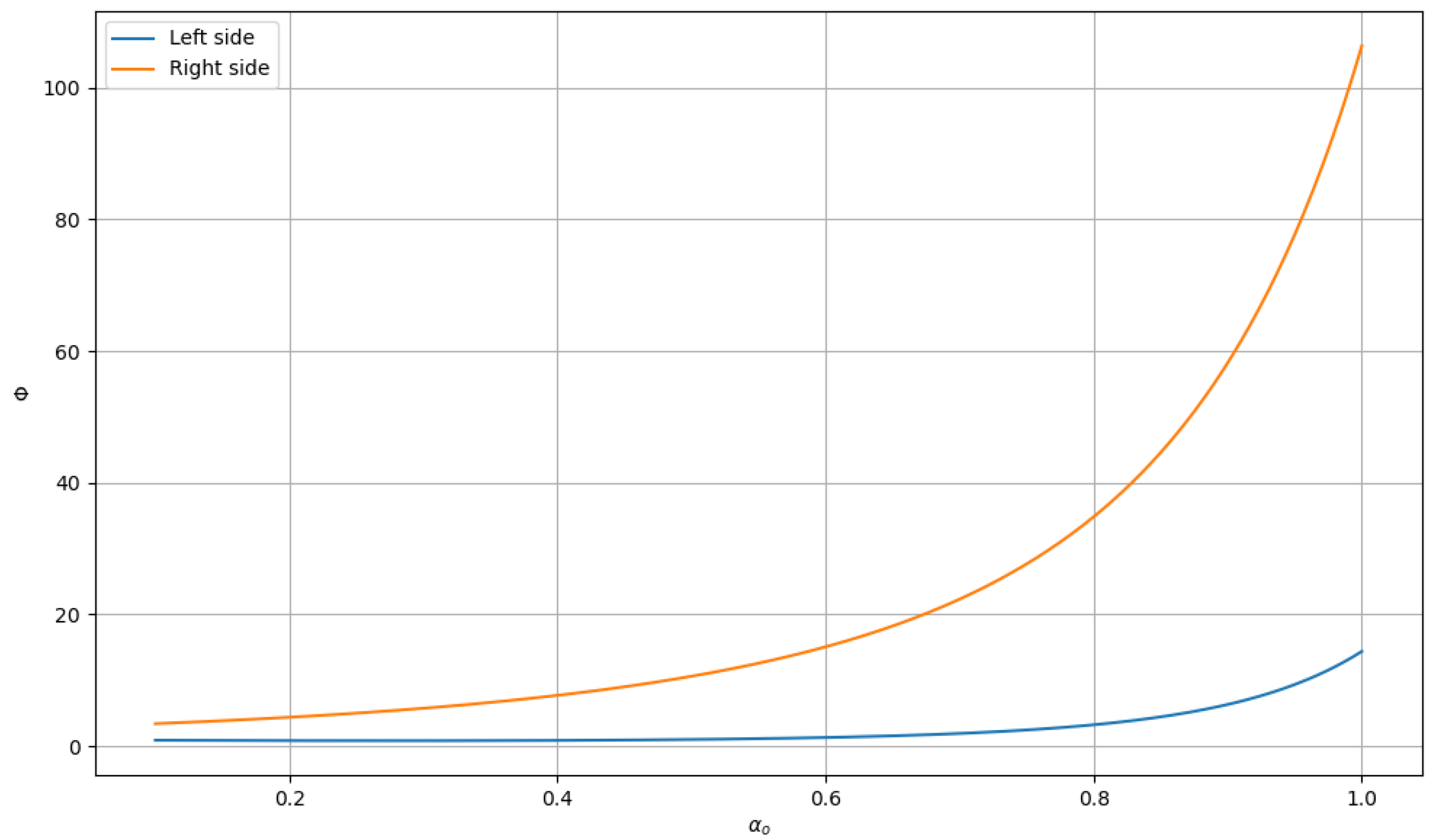
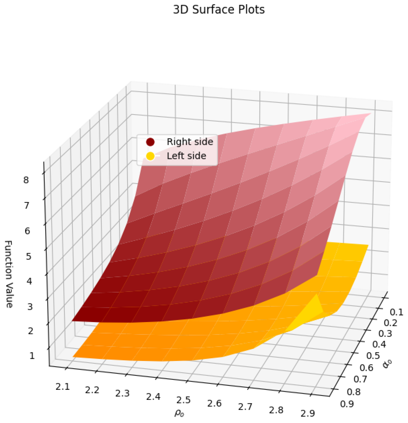
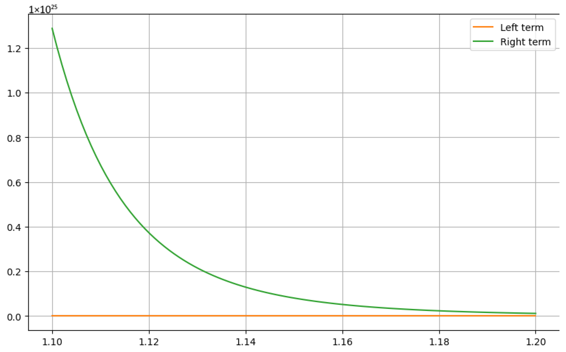
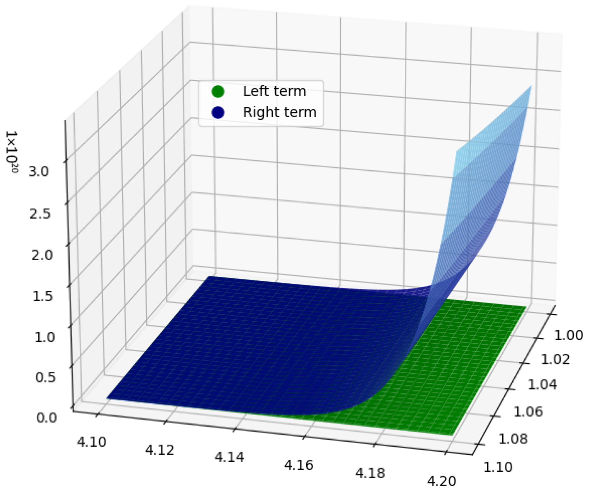
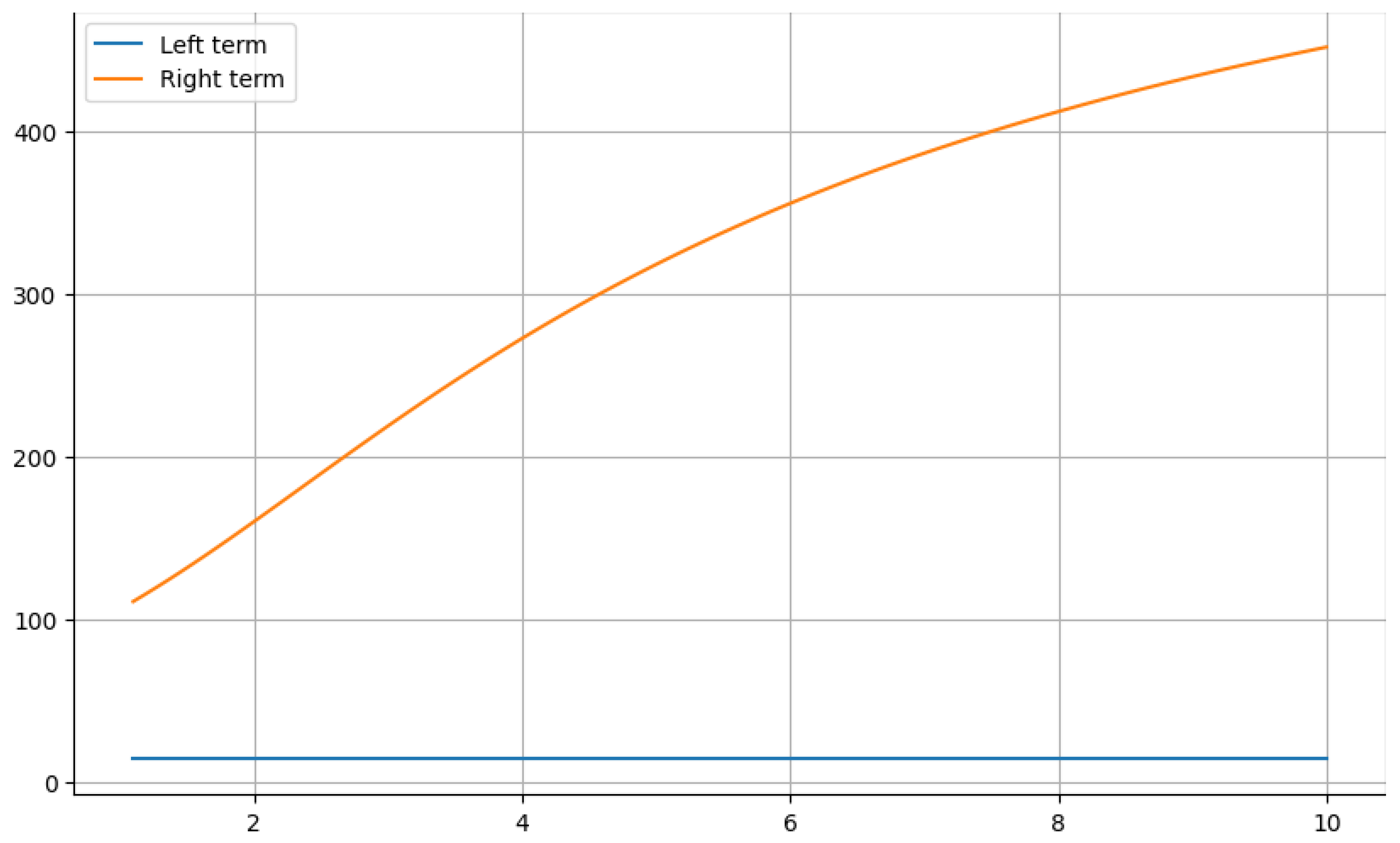
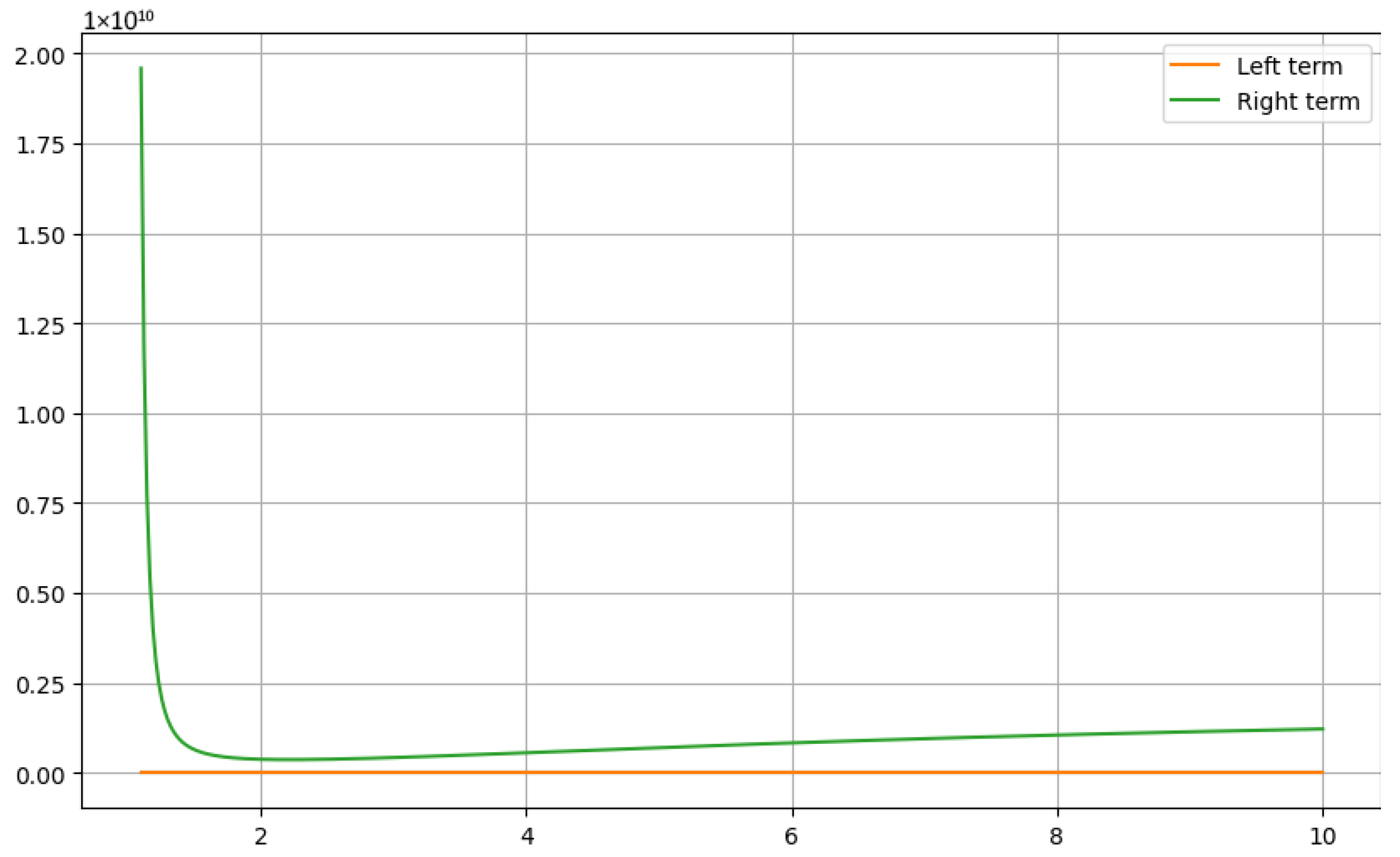
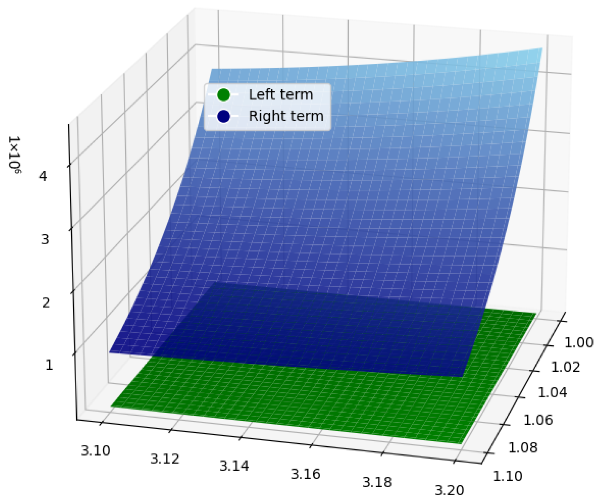
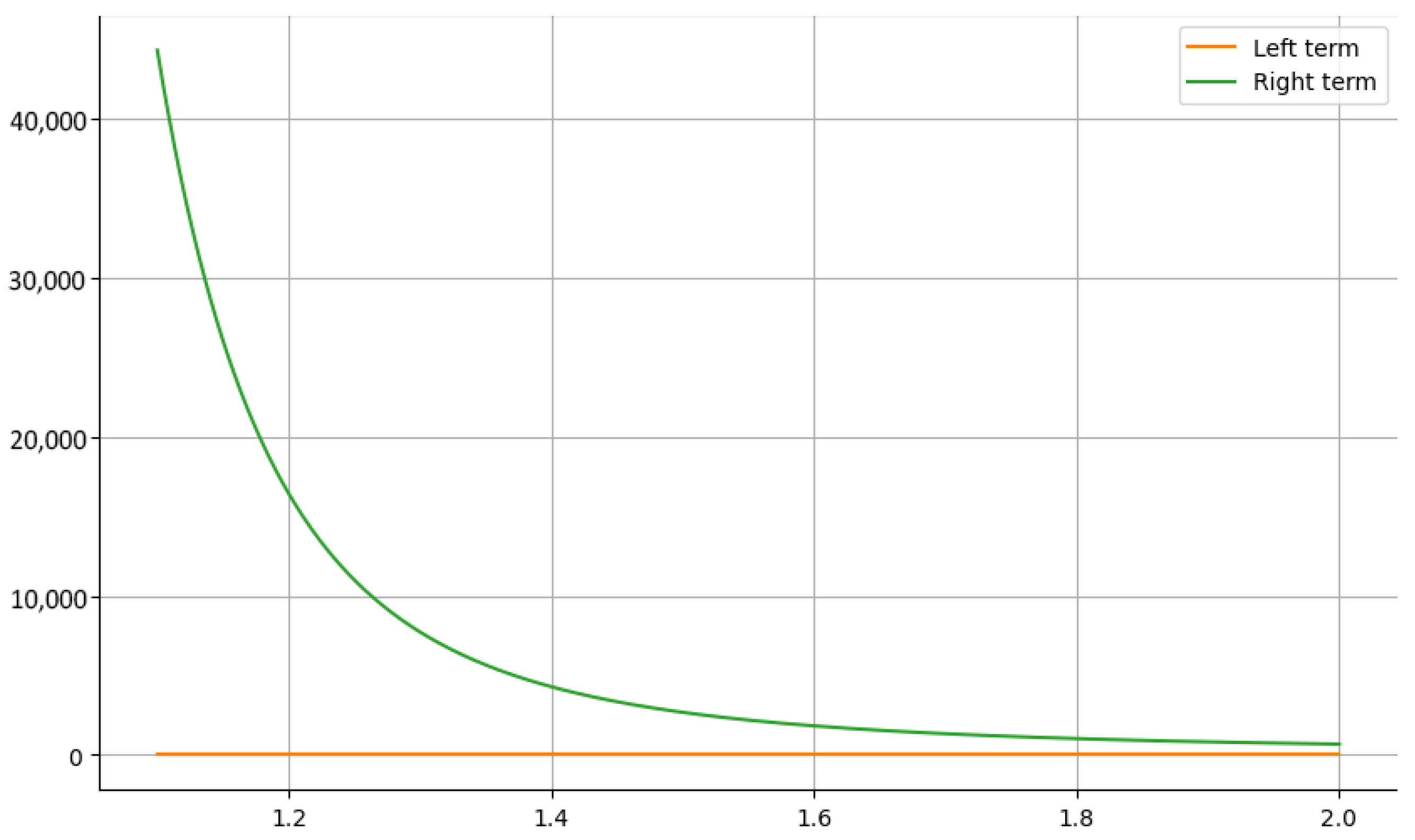
3. Comparison Examples with Graphical Analysis

In this section, making use of the improved version of Hölder–Yang’s integral inequality in Theorem 9, we obtain a smaller error bound than that in the original version of Theorem 7. Likewise, making use of the improved version of the generalized power-mean integral inequality in Theorem 10, we obtain a smaller error bound than that of the original version of Theorem 8. In this section, we shall demonstrate numerically that the altered forms of the Holder–Yang and generalized power-mean integral inequalities do present better methods than that of their original forms.

Example 6.

Let $\mathsf{ϝ}\left(\varkappa \right)=\frac{\mathrm{\Gamma }(1+5{\alpha }_o)}{\mathrm{\Gamma }(1+6{\alpha }_o)}{\varkappa }^{6{\alpha }_o},$ $\varkappa >0$. If we choose ${\sigma }_o=1,{\tau }_o=2,{\rho }_o=3,$ ${\lambda }_o=1={\mu }_o,$ ${\alpha }_o=1$ and ${\mathrm{q}}_{\mathrm{o}}=2,$, then the function $|{\mathsf{ϝ}}^{{\alpha }_o}\left(\varkappa \right)|={\varkappa }^{5{\alpha }_o}$ is convex for $\varkappa >0$. Here, we will determine the right part of the inequalities in Theorems 7 and 9 with $\eta \left({\tau }_o\right)={{\tau }_o}^{{\alpha }_o}$, then Corollaries 3 and 5 independently.

The right part of Corollary 3 will convert to

$$\begin{array}{cc}\hfill & {\left(\frac{1}{{\mathrm{p}}_{\mathrm{o}}+1}\right)}^{\frac{1}{{\mathrm{p}}_{\mathrm{o}}}}\left\{{\left(\frac{1}{2}|{\mathsf{ϝ}}^{\prime }\left({\tau }_o\right){|}^{{\mathrm{q}}_{\mathrm{o}}}+\frac{1}{2}{\left|{\mathsf{ϝ}}^{\prime }\left({\rho }_o\right)\right|}^{{\mathrm{q}}_{\mathrm{o}}}\right)}^{\frac{1}{{\mathrm{q}}_{\mathrm{o}}}}+{\left(\frac{1}{2}|{\mathsf{ϝ}}^{\prime }\left({\tau }_o\right){|}^{{\mathrm{q}}_{\mathrm{o}}}+\frac{1}{2}{\left|{\mathsf{ϝ}}^{\prime }\left({\sigma }_o\right)\right|}^{{\mathrm{q}}_{\mathrm{o}}}\right)}^{\frac{1}{{\mathrm{q}}_{\mathrm{o}}}}\right\}\hfill \\ \hfill & ={\left(\frac{1}{3}\right)}^{\frac{1}{2}}\left\{{\left(\frac{1}{2}\times 1024+\frac{1}{2}\times 59049\right)}^{\frac{1}{2}}+{\left(\frac{1}{2}\times 1024+\frac{1}{2}\times 1\right)}^{\frac{1}{2}}\right\}\hfill \\ \hfill & \approx 113.1311.\hfill \end{array}$$

The right part of Corollary 5 will convert to

$$\begin{array}{cc}\hfill & \{{\left(\frac{1}{{\mathrm{p}}_{\mathrm{o}}+2}\right)}^{\frac{1}{{\mathrm{p}}_{\mathrm{o}}}}{\left(\frac{1}{6}|{\mathsf{ϝ}}^{\prime }\left({\tau }_o\right){|}^{{\mathrm{q}}_{\mathrm{o}}}+\frac{1}{3}{\left|{\mathsf{ϝ}}^{\prime }\left({\rho }_o\right)\right|}^{{\mathrm{q}}_{\mathrm{o}}}\right)}^{\frac{1}{{\mathrm{q}}_{\mathrm{o}}}}\hfill \\ \hfill & +{\left(\frac{1}{({\mathrm{p}}_{\mathrm{o}}+1)({\mathrm{p}}_{\mathrm{o}}+2)}\right)}^{\frac{1}{{\mathrm{p}}_{\mathrm{o}}}}{\left(\frac{1}{3}|{\mathsf{ϝ}}^{\prime }\left({\tau }_o\right){|}^{{\mathrm{q}}_{\mathrm{o}}}+\frac{1}{6}{\left|{\mathsf{ϝ}}^{\prime }\left({\rho }_o\right)\right|}^{{\mathrm{q}}_{\mathrm{o}}}\right)}^{\frac{1}{{\mathrm{q}}_{\mathrm{o}}}}\}\hfill \\ \hfill & +\{{\left(\frac{1}{{\mathrm{p}}_{\mathrm{o}}+1}\right)}^{\frac{1}{{\mathrm{p}}_{\mathrm{o}}}}{\left(\frac{1}{6}|{\mathsf{ϝ}}^{\prime }\left({\tau }_o\right){|}^{{\mathrm{q}}_{\mathrm{o}}}+\frac{1}{3}{\left|{\mathsf{ϝ}}^{\prime }\left({\sigma }_o\right)\right|}^{{\mathrm{q}}_{\mathrm{o}}}\right)}^{\frac{1}{{\mathrm{q}}_{\mathrm{o}}}}\hfill \\ \hfill & +{\left(\frac{1}{({\mathrm{p}}_{\mathrm{o}}+1)({\mathrm{p}}_{\mathrm{o}}+2)}\right)}^{\frac{1}{{\mathrm{p}}_{\mathrm{o}}}}{\left(\frac{1}{3}|{\mathsf{ϝ}}^{\prime }\left({\tau }_o\right){|}^{{\mathrm{q}}_{\mathrm{o}}}+\frac{1}{6}{\left|{\mathsf{ϝ}}^{\prime }\left({\sigma }_o\right)\right|}^{{\mathrm{q}}_{\mathrm{o}}}\right)}^{\frac{1}{{\mathrm{q}}_{\mathrm{o}}}}\}\hfill \\ \hfill & =\left\{{\left(\frac{1}{4}\right)}^{\frac{1}{2}}{\left(\frac{1}{6}\times 1024+\frac{1}{3}\times 59049\right)}^{\frac{1}{2}}+{\left(\frac{1}{12}\right)}^{\frac{1}{2}}{\left(\frac{1}{3}\times 1024+\frac{1}{6}\times 59049\right)}^{\frac{1}{2}}\right\}\hfill \\ \hfill & +\left\{{\left(\frac{1}{4}\right)}^{\frac{1}{2}}{\left(\frac{1}{6}\times 1024+\frac{1}{3}\times 1\right)}^{\frac{1}{2}}+{\left(\frac{1}{12}\right)}^{\frac{1}{2}}{\left(\frac{1}{3}\times 1024+\frac{1}{6}\times 1\right)}^{\frac{1}{2}}\right\}\hfill \\ \hfill & \approx 111.4548.\hfill \end{array}$$

Obviously, 113.1311 > 111.4548, which validates that the error estimate inferred in Corollary 5 is bigger than that in Corollary 3.

Moreover, we choose ${\sigma }_o=1,{\tau }_o=2,{\rho }_o=3$ and ${\mathrm{q}}_{\mathrm{o}}\in [1.1,10]$, so the right-hand side of the Corollaries 3 and 5 will convert to

$$\begin{array}{cc}\hfill & {\mathfrak{F}}_{\mathfrak{1}}\left({\mathrm{q}}_{\mathrm{o}}\right)={\left(\frac{1}{{\mathrm{p}}_{\mathrm{o}}+1}\right)}^{\frac{1}{{\mathrm{p}}_{\mathrm{o}}}}\left\{{\left(\frac{1}{2}|{\mathsf{ϝ}}^{\prime }\left({\tau }_o\right){|}^{{\mathrm{q}}_{\mathrm{o}}}+\frac{1}{2}{\left|{\mathsf{ϝ}}^{\prime }\left({\rho }_o\right)\right|}^{{\mathrm{q}}_{\mathrm{o}}}\right)}^{\frac{1}{{\mathrm{q}}_{\mathrm{o}}}}+{\left(\frac{1}{2}|{\mathsf{ϝ}}^{\prime }\left({\tau }_o\right){|}^{{\mathrm{q}}_{\mathrm{o}}}+\frac{1}{2}{\left|{\mathsf{ϝ}}^{\prime }\left({\sigma }_o\right)\right|}^{{\mathrm{q}}_{\mathrm{o}}}\right)}^{\frac{1}{{\mathrm{q}}_{\mathrm{o}}}}\right\}\hfill \\ \hfill & ={\left(\frac{1}{{\mathrm{p}}_{\mathrm{o}}+1}\right)}^{\frac{1}{{\mathrm{p}}_{\mathrm{o}}}}\left\{{\left(\frac{1}{2}\times {\left|32\right|}^{{\mathrm{q}}_{\mathrm{o}}}+\frac{1}{2}\times {\left|243\right|}^{{\mathrm{q}}_{\mathrm{o}}}\right)}^{\frac{1}{{\mathrm{q}}_{\mathrm{o}}}}+{\left(\frac{1}{2}\times {\left|32\right|}^{{\mathrm{q}}_{\mathrm{o}}}+\frac{1}{2}\times {\left|1\right|}^{{\mathrm{q}}_{\mathrm{o}}}\right)}^{\frac{1}{{\mathrm{q}}_{\mathrm{o}}}}\right\},\hfill \end{array}$$

and

$$\begin{array}{cc}\hfill & {\mathfrak{F}}_{\mathfrak{2}}\left({\mathrm{q}}_{\mathrm{o}}\right)=\{{\left(\frac{1}{{\mathrm{p}}_{\mathrm{o}}+2}\right)}^{\frac{1}{{\mathrm{p}}_{\mathrm{o}}}}{\left(\frac{1}{6}|{\mathsf{ϝ}}^{\prime }\left({\tau }_o\right){|}^{{\mathrm{q}}_{\mathrm{o}}}+\frac{1}{3}{\left|{\mathsf{ϝ}}^{\prime }\left({\rho }_o\right)\right|}^{{\mathrm{q}}_{\mathrm{o}}}\right)}^{\frac{1}{{\mathrm{q}}_{\mathrm{o}}}}\hfill \\ \hfill & +{\left(\frac{1}{({\mathrm{p}}_{\mathrm{o}}+1)({\mathrm{p}}_{\mathrm{o}}+2)}\right)}^{\frac{1}{{\mathrm{p}}_{\mathrm{o}}}}{\left(\frac{1}{3}|{\mathsf{ϝ}}^{\prime }\left({\tau }_o\right){|}^{{\mathrm{q}}_{\mathrm{o}}}+\frac{1}{6}{\left|{\mathsf{ϝ}}^{\prime }\left({\rho }_o\right)\right|}^{{\mathrm{q}}_{\mathrm{o}}}\right)}^{\frac{1}{{\mathrm{q}}_{\mathrm{o}}}}\}\hfill \\ \hfill & +\{{\left(\frac{1}{{\mathrm{p}}_{\mathrm{o}}+1}\right)}^{\frac{1}{{\mathrm{p}}_{\mathrm{o}}}}{\left(\frac{1}{6}|{\mathsf{ϝ}}^{\prime }\left({\tau }_o\right){|}^{{\mathrm{q}}_{\mathrm{o}}}+\frac{1}{3}{\left|{\mathsf{ϝ}}^{\prime }\left({\sigma }_o\right)\right|}^{{\mathrm{q}}_{\mathrm{o}}}\right)}^{\frac{1}{{\mathrm{q}}_{\mathrm{o}}}}\hfill \\ \hfill & +{\left(\frac{1}{({\mathrm{p}}_{\mathrm{o}}+1)({\mathrm{p}}_{\mathrm{o}}+2)}\right)}^{\frac{1}{{\mathrm{p}}_{\mathrm{o}}}}{\left(\frac{1}{3}|{\mathsf{ϝ}}^{\prime }\left({\tau }_o\right){|}^{{\mathrm{q}}_{\mathrm{o}}}+\frac{1}{6}{\left|{\mathsf{ϝ}}^{\prime }\left({\sigma }_o\right)\right|}^{{\mathrm{q}}_{\mathrm{o}}}\right)}^{\frac{1}{{\mathrm{q}}_{\mathrm{o}}}}\}\hfill \\ \hfill & =\{{\left(\frac{1}{{\mathrm{p}}_{\mathrm{o}}+2}\right)}^{\frac{1}{{\mathrm{p}}_{\mathrm{o}}}}{\left(\frac{1}{6}\times {\left|32\right|}^{{\mathrm{q}}_{\mathrm{o}}}+\frac{1}{3}\times {\left|243\right|}^{{\mathrm{q}}_{\mathrm{o}}}\right)}^{\frac{1}{{\mathrm{q}}_{\mathrm{o}}}}\hfill \\ \hfill & +{\left(\frac{1}{({\mathrm{p}}_{\mathrm{o}}+1)({\mathrm{p}}_{\mathrm{o}}+2)}\right)}^{\frac{1}{{\mathrm{p}}_{\mathrm{o}}}}{\left(\frac{1}{3}\times {\left|32\right|}^{{\mathrm{q}}_{\mathrm{o}}}+\frac{1}{6}\times {\left|243\right|}^{{\mathrm{q}}_{\mathrm{o}}}\right)}^{\frac{1}{{\mathrm{q}}_{\mathrm{o}}}}\}\hfill \\ \hfill & +\{{\left(\frac{1}{{\mathrm{p}}_{\mathrm{o}}+2}\right)}^{\frac{1}{{\mathrm{p}}_{\mathrm{o}}}}{\left(\frac{1}{6}\times {\left|32\right|}^{{\mathrm{q}}_{\mathrm{o}}}+\frac{1}{3}\times {\left|1\right|}^{{\mathrm{q}}_{\mathrm{o}}}\right)}^{\frac{1}{{\mathrm{q}}_{\mathrm{o}}}}\hfill \\ \hfill & +{\left(\frac{1}{({\mathrm{p}}_{\mathrm{o}}+1)({\mathrm{p}}_{\mathrm{o}}+2)}\right)}^{\frac{1}{{\mathrm{p}}_{\mathrm{o}}}}{\left(\frac{1}{3}\times {\left|32\right|}^{{\mathrm{q}}_{\mathrm{o}}}+\frac{1}{6}\times {\left|1\right|}^{{\mathrm{q}}_{\mathrm{o}}}\right)}^{\frac{1}{{\mathrm{q}}_{\mathrm{o}}}}\},\hfill \end{array}$$

where $\frac{1}{{\mathrm{p}}_{\mathrm{o}}}+\frac{1}{{\mathrm{q}}_{\mathrm{o}}}=1.$ Drawing the graphical analysis in Figure 11 shows the upper bound deduced in Corollary 5 is bigger than that in Corollary 3.

Example 7.

Let $\mathsf{ϝ}\left(\varkappa \right)=\frac{\mathrm{\Gamma }(1+5{\alpha }_o)}{\mathrm{\Gamma }(1+6{\alpha }_o)}{\varkappa }^{6{\alpha }_o},$ $\varkappa >0$. If we choose ${\sigma }_o=1,{\tau }_o=2,{\rho }_o=3,$ ${\lambda }_o=1={\mu }_o,$ ${\alpha }_o=1$ and ${\mathrm{q}}_{\mathrm{o}}=2$, then the function $|{\mathsf{ϝ}}^{{\alpha }_o}\left(\varkappa \right)|={\varkappa }^{5{\alpha }_o}$ is convex for $\varkappa >0$. Here, we calculate the right part of the inequalities in Theorems 8 and 10 with $\eta \left({\tau }_o\right)={{\tau }_o}^{{\alpha }_o}$, then Corollaries 4 and 6 independently.

The right part of Corollary 4 will convert to

$$\begin{array}{cc}\hfill & {\left(\frac{1}{2}\right)}^{1-\frac{1}{{\mathrm{q}}_{\mathrm{o}}}}\left\{{\left(\frac{1}{6}|{\mathsf{ϝ}}^{\prime }\left({\tau }_o\right){|}^{{\mathrm{q}}_{\mathrm{o}}}+\frac{1}{3}{\left|{\mathsf{ϝ}}^{\prime }\left({\rho }_o\right)\right|}^{{\mathrm{q}}_{\mathrm{o}}}\right)}^{\frac{1}{{\mathrm{q}}_{\mathrm{o}}}}+{\left(\frac{1}{6}|{\mathsf{ϝ}}^{\prime }\left({\tau }_o\right){|}^{{\mathrm{q}}_{\mathrm{o}}}+\frac{1}{3}{\left|{\mathsf{ϝ}}^{\prime }\left({\sigma }_o\right)\right|}^{{\mathrm{q}}_{\mathrm{o}}}\right)}^{\frac{1}{{\mathrm{q}}_{\mathrm{o}}}}\right\}\hfill \\ \hfill & ={\left(\frac{1}{2}\right)}^{1-\frac{1}{2}}\left\{{\left(\frac{1}{6}\times 1024+\frac{1}{3}\times 59049\right)}^{\frac{1}{2}}+{\left(\frac{1}{6}\times 1024+\frac{1}{3}\times 1\right)}^{\frac{1}{2}}\right\},\hfill \\ \hfill & \approx 108.8801.\hfill \end{array}$$

The right part of Corollary 6 will convert to

$$\begin{array}{cc}\hfill & \{{\left(\frac{1}{3}\right)}^{1-\frac{1}{{\mathrm{q}}_{\mathrm{o}}}}{\left(\frac{1}{12}|{\mathsf{ϝ}}^{\prime }\left({\tau }_o\right){|}^{{\mathrm{q}}_{\mathrm{o}}}+\frac{1}{4}{\left|{\mathsf{ϝ}}^{\prime }\left({\rho }_o\right)\right|}^{{\mathrm{q}}_{\mathrm{o}}}\right)}^{\frac{1}{{\mathrm{q}}_{\mathrm{o}}}}\hfill \\ \hfill & +{\left(\frac{1}{6}\right)}^{1-\frac{1}{{\mathrm{q}}_{\mathrm{o}}}}{\left(\frac{1}{12}|{\mathsf{ϝ}}^{\prime }\left({\tau }_o\right){|}^{{\mathrm{q}}_{\mathrm{o}}}+\frac{1}{12}{\left|{\mathsf{ϝ}}^{\prime }\left({\rho }_o\right)\right|}^{{\mathrm{q}}_{\mathrm{o}}}\right)}^{\frac{1}{{\mathrm{q}}_{\mathrm{o}}}}\}\hfill \\ \hfill & +\{{\left(\frac{1}{3}\right)}^{1-\frac{1}{{\mathrm{p}}_{\mathrm{o}}}}{\left(\frac{1}{12}|{\mathsf{ϝ}}^{\prime }\left({\tau }_o\right){|}^{{\mathrm{q}}_{\mathrm{o}}}+\frac{1}{4}{\left|{\mathsf{ϝ}}^{\prime }\left({\sigma }_o\right)\right|}^{{\mathrm{q}}_{\mathrm{o}}}\right)}^{\frac{1}{{\mathrm{q}}_{\mathrm{o}}}}\hfill \\ \hfill & +{\left(\frac{1}{6}\right)}^{1-\frac{1}{{\mathrm{q}}_{\mathrm{o}}}}{\left(\frac{1}{12}|{\mathsf{ϝ}}^{\prime }\left({\tau }_o\right){|}^{{\mathrm{q}}_{\mathrm{o}}}+\frac{1}{12}{\left|{\mathsf{ϝ}}^{\prime }\left({\sigma }_o\right)\right|}^{{\mathrm{q}}_{\mathrm{o}}}\right)}^{\frac{1}{{\mathrm{q}}_{\mathrm{o}}}}\}\hfill \\ \hfill & =\{{\left(\frac{1}{3}\right)}^{\frac{1}{2}}{\left(\frac{1}{12}\times 1024+\frac{1}{4}\times 59049\right)}^{\frac{1}{2}}\hfill \\ \hfill & +{\left(\frac{1}{6}\right)}^{\frac{1}{2}}{\left(\frac{1}{12}\times 1024+\frac{1}{12}\times 59049\right)}^{\frac{1}{2}}\}\hfill \\ \hfill & +\{{\left(\frac{1}{3}\right)}^{\frac{1}{2}}{\left(\frac{1}{12}\times 1024+\frac{1}{4}\times 1\right)}^{\frac{1}{2}}\hfill \\ \hfill & +{\left(\frac{1}{6}\right)}^{\frac{1}{2}}{\left(\frac{1}{12}\times 1024+\frac{1}{12}\times 1\right)}^{\frac{1}{2}}\},\hfill \\ \hfill & \approx 108.3498.\hfill \end{array}$$

Obviously, 108.8801 > 108.3498, which validates that the error estimate inferred in Corollary 6 is bigger than that Corollary 4.

Moreover, we choose ${\tau }_o=2,{\mathrm{q}}_{\mathrm{o}}=2,{\sigma }_o\in [1,2]$ and ${\rho }_o\in [3,4]$, so the right-hand side of the Corollaries 4 and 6 will convert to

$$\begin{array}{cc}\hfill & {\mathfrak{G}}_{\mathfrak{1}}({\sigma }_o,{\rho }_o)={\left(\frac{1}{2}\right)}^{1-\frac{1}{{\mathrm{q}}_{\mathrm{o}}}}\left\{{\left(\frac{1}{6}|{\mathsf{ϝ}}^{\prime }\left({\tau }_o\right){|}^{{\mathrm{q}}_{\mathrm{o}}}+\frac{1}{3}{\left|{\mathsf{ϝ}}^{\prime }\left({\rho }_o\right)\right|}^{{\mathrm{q}}_{\mathrm{o}}}\right)}^{\frac{1}{{\mathrm{q}}_{\mathrm{o}}}}+{\left(\frac{1}{6}|{\mathsf{ϝ}}^{\prime }\left({\tau }_o\right){|}^{{\mathrm{q}}_{\mathrm{o}}}+\frac{1}{3}{\left|{\mathsf{ϝ}}^{\prime }\left({\sigma }_o\right)\right|}^{{\mathrm{q}}_{\mathrm{o}}}\right)}^{\frac{1}{{\mathrm{q}}_{\mathrm{o}}}}\right\},\hfill \\ \hfill & ={\left(\frac{1}{2}\right)}^{1-\frac{1}{2}}\left\{{\left(\frac{1}{6}\times {\left|32\right|}^2+\frac{1}{2}\times {\left|{\rho }_o\right|}^2\right)}^{\frac{1}{2}}+{\left(\frac{1}{2}\times {\left|32\right|}^2+\frac{1}{2}\times {\left|{\sigma }_o\right|}^2\right)}^{\frac{1}{2}}\right\},\hfill \end{array}$$

and

$$\begin{array}{cc}\hfill & {\mathfrak{G}}_{\mathfrak{2}}({\sigma }_o,{\rho }_o)=\{{\left(\frac{1}{3}\right)}^{1-\frac{1}{{\mathrm{q}}_{\mathrm{o}}}}{\left(\frac{1}{12}|{\mathsf{ϝ}}^{\prime }\left({\tau }_o\right){|}^{{\mathrm{q}}_{\mathrm{o}}}+\frac{1}{4}{\left|{\mathsf{ϝ}}^{\prime }\left({\rho }_o\right)\right|}^{{\mathrm{q}}_{\mathrm{o}}}\right)}^{\frac{1}{{\mathrm{q}}_{\mathrm{o}}}}\hfill \\ \hfill & +{\left(\frac{1}{6}\right)}^{1-\frac{1}{{\mathrm{q}}_{\mathrm{o}}}}{\left(\frac{1}{12}|{\mathsf{ϝ}}^{\prime }\left({\tau }_o\right){|}^{{\mathrm{q}}_{\mathrm{o}}}+\frac{1}{12}{\left|{\mathsf{ϝ}}^{\prime }\left({\rho }_o\right)\right|}^{{\mathrm{q}}_{\mathrm{o}}}\right)}^{\frac{1}{{\mathrm{q}}_{\mathrm{o}}}}\}\hfill \\ \hfill & +\{{\left(\frac{1}{3}\right)}^{1-\frac{1}{{\mathrm{q}}_{\mathrm{o}}}}{\left(\frac{1}{12}|{\mathsf{ϝ}}^{\prime }\left({\tau }_o\right){|}^{{\mathrm{q}}_{\mathrm{o}}}+\frac{1}{4}{\left|{\mathsf{ϝ}}^{\prime }\left({\sigma }_o\right)\right|}^{{\mathrm{q}}_{\mathrm{o}}}\right)}^{\frac{1}{{\mathrm{q}}_{\mathrm{o}}}}\hfill \\ \hfill & +{\left(\frac{1}{6}\right)}^{1-\frac{1}{{\mathrm{q}}_{\mathrm{o}}}}{\left(\frac{1}{12}|{\mathsf{ϝ}}^{\prime }\left({\tau }_o\right){|}^{{\mathrm{q}}_{\mathrm{o}}}+\frac{1}{12}{\left|{\mathsf{ϝ}}^{\prime }\left({\sigma }_o\right)\right|}^{{\mathrm{q}}_{\mathrm{o}}}\right)}^{\frac{1}{{\mathrm{q}}_{\mathrm{o}}}}\},\hfill \\ \hfill & =\left\{{\left(\frac{1}{3}\right)}^{\frac{1}{2}}{\left(\frac{1}{12}\times {\left|32\right|}^2+\frac{1}{4}\times {\left|{{\rho }_o}^5\right|}^2\right)}^{\frac{1}{2}}+{\left(\frac{1}{6}\right)}^{\frac{1}{2}}{\left(\frac{1}{12}\times {\left|32\right|}^2+\frac{1}{12}\times {\left|{{\rho }_o}^5\right|}^2\right)}^{\frac{1}{2}}\right\}\hfill \\ \hfill & +\left\{{\left(\frac{1}{3}\right)}^{\frac{1}{2}}{\left(\frac{1}{12}\times {\left|32\right|}^{{\mathrm{q}}_{\mathrm{o}}}+\frac{1}{4}\times {\left|{{\sigma }_o}^5\right|}^2\right)}^{\frac{1}{2}}+{\left(\frac{1}{6}\right)}^{\frac{1}{2}}{\left(\frac{1}{12}\times {\left|32\right|}^2+\frac{1}{12}\times {\left|{{\sigma }_o}^5\right|}^2\right)}^{\frac{1}{2}}\right\}.\hfill \end{array}$$

Drawing the graphical analysis in Figure 12 shows the upper bound deduced in Corollary 6 is bigger than that in Corollary 4.

All Figures in this paper were created with Python version (3.12.3), using the Matplotlib (3.10.0) and NumPy (2.3.0) libraries for numerical computation and visualization.

4. Applications

In this section, we provide some novel applications of our primary findings.

4.1. Special Means over Fractal Sets

In the framework of fractal space, the aforementioned process determined the n-lograithmic means and ${\alpha }_o$-like special means if $0<{\sigma }_o<{\rho }_o.$

(1)

The generalized arithmetic mean:

$$\begin{array}{cc}\hfill & {\mathrm{A}}_{{\alpha }_o}({\sigma }_o,{\rho }_o)=\frac{{{\sigma }_o}^{{\alpha }_o}+{{\rho }_o}^{{\alpha }_o}}{2^{{\alpha }_o}}.\hfill \end{array}$$

(2)

The generalized n-logarithmic mean:

$$\begin{array}{cc}\hfill & {\mathrm{L}}_{\mathrm{n}}{\alpha }_o({\sigma }_o,{\rho }_o)={\left[\frac{\mathrm{\Gamma }(1+\mathrm{n}{\alpha }_o)}{\mathrm{\Gamma }(1+(\mathrm{n}+1){\alpha }_o)}\frac{{\left({\rho }_o\right)}^{(\mathrm{n}+1){\alpha }_o}-{\left({\sigma }_o\right)}^{(\mathrm{n}+1){\alpha }_o}}{{({\rho }_o-{\sigma }_o)}^{{\alpha }_o}}\right]}^{\frac{1}{\mathrm{n}}},\hfill \end{array}$$

where $\mathrm{n}\in \mathbb{Z}\setminus$ $\{-1,0\},$ ${\sigma }_o,{\rho }_o\in \mathbb{R},$ ${\sigma }_o={\rho }_o.$

Proposition 1.

For $0<{\sigma }_o<{\rho }_o,$ ${\alpha }_o\in (0,1]$ and $\mathrm{n}\ge 1.$ If all conditions listed in Corollary 2 are satisfied with ${\lambda }_o=0={\mu }_o$ and ${\tau }_o=\frac{{\sigma }_o+{\rho }_o}{2}$, then we have

$$\begin{array}{cc}\hfill & |\frac{\mathrm{\Gamma }(1+\mathfrak{u}{\alpha }_o)}{\mathrm{\Gamma }(1+(\mathfrak{u}+1){\alpha }_o)}{\left({\mathrm{A}}_{{\alpha }_o}({\sigma }_o,{\rho }_o)\right)}^{(\mathfrak{u}+1)}-\frac{\mathrm{\Gamma }(1+{\alpha }_o)\mathrm{\Gamma }(1+\mathfrak{u}{\alpha }_o)}{\mathrm{\Gamma }(1+(\mathfrak{u}+1){\alpha }_o)}{\mathrm{L}}_{(\mathfrak{u}+1){\alpha }_o}^{(\mathfrak{u}+1)}({\sigma }_o,{\rho }_o)|\hfill \\ \hfill & \le \frac{{({\rho }_o-{\sigma }_o)}^{2{\alpha }_o}}{4^{{\alpha }_o}}\{\left(\frac{\mathrm{\Gamma }(1+{\alpha }_o)}{\mathrm{\Gamma }(1+2{\alpha }_o)}-\frac{\mathrm{\Gamma }(1+2{\alpha }_o)}{\mathrm{\Gamma }(1+3{\alpha }_o)}\right)\left[{\left({\rho }_o\right)}^{\mathfrak{u}{\alpha }_o}+{\left({\sigma }_o\right)}^{\mathfrak{u}{\alpha }_o}\right]\hfill \\ \hfill & +\frac{2^{{\alpha }_o}\mathrm{\Gamma }(1+2{\alpha }_o)}{\mathrm{\Gamma }(1+3{\alpha }_o)}{\left({\mathrm{A}}_{{\alpha }_o}({\sigma }_o,{\rho }_o)\right)}^{\left(\mathfrak{u}\right)}\}.\hfill \end{array}$$

Proof. 

We choose the function $\mathsf{ϝ}:\mathrm{I}=(0,\infty )\to {\mathbb{R}}^{{\alpha }_o},$ $\mathsf{ϝ}\left(\varkappa \right)=\frac{\mathrm{\Gamma }(1+\mathfrak{u}{\alpha }_o)}{\mathrm{\Gamma }(1+(\mathfrak{u}+1){\alpha }_o)}{\varkappa }^{(\mathfrak{u}+1){\alpha }_o}$ and its derivative ${\mathsf{ϝ}}^{{\alpha }_o}\left(\varkappa \right)={\varkappa }^{\mathfrak{u}{\alpha }_o}$; both are non-negative generalized convex functions under the interval $(0,+\infty ).$ So we have

$$\begin{array}{cc}\hfill & \mathsf{ϝ}\left({\sigma }_o\right)=\frac{\mathrm{\Gamma }(1+\mathfrak{u}{\alpha }_o)}{\mathrm{\Gamma }(1+(\mathfrak{u}+1){\alpha }_o)}{{\sigma }_o}^{(\mathfrak{u}+1){\alpha }_o},\left|{\mathsf{ϝ}}^{{\alpha }_o}\left({\sigma }_o\right)\right|={\left({\sigma }_o\right)}^{\mathfrak{u}{\alpha }_o},\hfill \\ \hfill & \mathsf{ϝ}\left({\rho }_o\right)=\frac{\mathrm{\Gamma }(1+\mathfrak{u}{\alpha }_o)}{\mathrm{\Gamma }(1+(\mathfrak{u}+1){\alpha }_o)}{{\rho }_o}^{(\mathfrak{u}+1){\alpha }_o},\left|{\mathsf{ϝ}}^{{\alpha }_o}\left({\rho }_o\right)\right|={\left({\rho }_o\right)}^{\mathfrak{u}{\alpha }_o},\hfill \\ \hfill & \mathsf{ϝ}\left(\frac{{\sigma }_o+{\rho }_o}{2}\right)=\frac{\mathrm{\Gamma }(1+\mathfrak{u}{\alpha }_o)}{\mathrm{\Gamma }(1+(\mathfrak{u}+1){\alpha }_o)}{\left(\frac{{\sigma }_o+{\rho }_o}{2}\right)}^{(\mathfrak{u}+1){\alpha }_o}=\frac{\mathrm{\Gamma }(1+\mathfrak{u}{\alpha }_o)}{\mathrm{\Gamma }(1+(\mathfrak{u}+1){\alpha }_o)}{\left({\mathrm{A}}_{{\alpha }_o}({\sigma }_o,{\rho }_o)\right)}^{(\mathfrak{u}+1)},\hfill \\ \hfill & \left|{\mathsf{ϝ}}^{{\alpha }_o}\left(\frac{{\sigma }_o+{\rho }_o}{2}\right)\right|={\left(\frac{{\sigma }_o+{\rho }_o}{2}\right)}^{\mathfrak{u}{\alpha }_o}{\left({\mathrm{A}}_{{\alpha }_o}({\sigma }_o,{\rho }_o)\right)}^{\left(\mathfrak{u}\right)},\hfill \\ \hfill and\\ \hfill & \frac{\mathrm{\Gamma }(1+{\alpha }_o)}{{({\rho }_o-{\sigma }_o)}^{{\alpha }_o}}{}_{{\sigma }_o}\mathrm{I}_{{\rho }_o}^{{\alpha }_o}\mathsf{ϝ}\left(\varkappa \right)=\frac{\mathrm{\Gamma }(1+{\alpha }_o)\mathrm{\Gamma }(1+\mathfrak{u}{\alpha }_o)}{\mathrm{\Gamma }(1+(\mathfrak{u}+1){\alpha }_o)}{\mathrm{L}}_{(\mathfrak{u}+1){\alpha }_o}^{(\mathfrak{u}+1)}({\sigma }_o,{\rho }_o).\hfill \end{array}$$

By employing the above-mentioned values and definition of special means in Corollary 2, we can obtained the expected result. □

Proposition 2.

For $0<{\sigma }_o<{\rho }_o,$ ${\alpha }_o\in (0,1]$ and $\mathrm{n}\ge 1.$ If all conditions listed in Corollary 2 are satisfied with ${\lambda }_o=\frac{1}{3}={\mu }_o$ and ${\tau }_o=\frac{{\sigma }_o+{\rho }_o}{2}$, then we have

$$\begin{array}{cc}\hfill & |\frac{1^{{\alpha }_o}}{6^{{\alpha }_o}}\frac{\mathrm{\Gamma }(1+\mathfrak{u}{\alpha }_o)}{\mathrm{\Gamma }(1+(\mathfrak{u}+1){\alpha }_o)}\left[{\left({\rho }_o\right)}^{(\mathfrak{u}+1){\alpha }_o}+4{\left({\mathrm{A}}_{{\alpha }_o}({\sigma }_o,{\rho }_o)\right)}^{(\mathfrak{u}+1)}+{\left({\sigma }_o\right)}^{(\mathfrak{u}+1){\alpha }_o}\right]\hfill \\ \hfill & -\frac{\mathrm{\Gamma }(1+{\alpha }_o)\mathrm{\Gamma }(1+\mathfrak{u}{\alpha }_o)}{\mathrm{\Gamma }(1+(\mathfrak{u}+1){\alpha }_o)}{\mathrm{L}}_{(\mathfrak{u}+1){\alpha }_o}^{(\mathfrak{u}+1)}({\sigma }_o,{\rho }_o)|\hfill \\ \hfill & \le \frac{{({\rho }_o-{\sigma }_o)}^{2{\alpha }_o}}{4^{{\alpha }_o}}\hfill \\ \hfill & \times \{\left(\frac{1^{{\alpha }_o}}{\mathrm{\Gamma }(1+{\alpha }_o)}\left(-\frac{1^{{\alpha }_o}}{9^{{\alpha }_o}}\right)+\frac{{28}^{{\alpha }_o}}{{27}^{{\alpha }_o}}\frac{\mathrm{\Gamma }(1+{\alpha }_o)}{\mathrm{\Gamma }(1+2{\alpha }_o)}+\frac{\mathrm{\Gamma }(1+2{\alpha }_o)}{\mathrm{\Gamma }(1+3{\alpha }_o)}\left(-\frac{{25}^{{\alpha }_o}}{{27}^{{\alpha }_o}}\right)\right)\left[{\left({\rho }_o\right)}^{\mathfrak{u}{\alpha }_o}+{\left({\sigma }_o\right)}^{\mathfrak{u}{\alpha }_o}\right]\hfill \\ \hfill & +2^{{\alpha }_o}{\left({\mathrm{A}}_{{\alpha }_o}({\sigma }_o,{\rho }_o)\right)}^{\left(\mathfrak{u}\right)}\left(\frac{{25}^{{\alpha }_o}}{{27}^{{\alpha }_o}}\frac{\mathrm{\Gamma }(1+2{\alpha }_o)}{\mathrm{\Gamma }(1+3{\alpha }_o)}-\frac{7^{{\alpha }_o}}{{27}^{{\alpha }_o}}\frac{\mathrm{\Gamma }(1+{\alpha }_o)}{\mathrm{\Gamma }(1+2{\alpha }_o)}\right)\}.\hfill \end{array}$$

Proof. 

We choose the function $\mathsf{ϝ}:\mathrm{I}=(0,\infty )\to {\mathbb{R}}^{{\alpha }_o},$ $\mathsf{ϝ}\left(\varkappa \right)=\frac{\mathrm{\Gamma }(1+\mathfrak{u}{\alpha }_o)}{\mathrm{\Gamma }(1+(\mathfrak{u}+1){\alpha }_o)}{\varkappa }^{(\mathfrak{u}+1){\alpha }_o}$ and its derivative ${\mathsf{ϝ}}^{{\alpha }_o}\left(\varkappa \right)={\varkappa }^{\mathfrak{u}{\alpha }_o}$; both are non-negative generalized convex functions under the interval $(0,+\infty ).$ So we have

$$\begin{array}{cc}\hfill & \mathsf{ϝ}\left({\sigma }_o\right)=\frac{\mathrm{\Gamma }(1+\mathfrak{u}{\alpha }_o)}{\mathrm{\Gamma }(1+(\mathfrak{u}+1){\alpha }_o)}{{\sigma }_o}^{(\mathfrak{u}+1){\alpha }_o},\left|{\mathsf{ϝ}}^{{\alpha }_o}\left({\sigma }_o\right)\right|={\left({\sigma }_o\right)}^{\mathfrak{u}{\alpha }_o},\hfill \\ \hfill & \mathsf{ϝ}\left({\rho }_o\right)=\frac{\mathrm{\Gamma }(1+\mathfrak{u}{\alpha }_o)}{\mathrm{\Gamma }(1+(\mathfrak{u}+1){\alpha }_o)}{{\rho }_o}^{(\mathfrak{u}+1){\alpha }_o},\left|{\mathsf{ϝ}}^{{\alpha }_o}\left({\rho }_o\right)\right|={\left({\rho }_o\right)}^{\mathfrak{u}{\alpha }_o},\hfill \\ \hfill & \mathsf{ϝ}\left(\frac{{\sigma }_o+{\rho }_o}{2}\right)=\frac{\mathrm{\Gamma }(1+\mathfrak{u}{\alpha }_o)}{\mathrm{\Gamma }(1+(\mathfrak{u}+1){\alpha }_o)}{\left(\frac{{\sigma }_o+{\rho }_o}{2}\right)}^{(\mathfrak{u}+1){\alpha }_o}=\frac{\mathrm{\Gamma }(1+\mathfrak{u}{\alpha }_o)}{\mathrm{\Gamma }(1+(\mathfrak{u}+1){\alpha }_o)}{\left({\mathrm{A}}_{{\alpha }_o}({\sigma }_o,{\rho }_o)\right)}^{(\mathfrak{u}+1)},\hfill \\ \hfill & \left|{\mathsf{ϝ}}^{{\alpha }_o}\left(\frac{{\sigma }_o+{\rho }_o}{2}\right)\right|={\left(\frac{{\sigma }_o+{\rho }_o}{2}\right)}^{\mathfrak{u}{\alpha }_o}{\left({\mathrm{A}}_{{\alpha }_o}({\sigma }_o,{\rho }_o)\right)}^{\left(\mathfrak{u}\right)},\hfill \\ \hfill and\\ \hfill & \frac{\mathrm{\Gamma }(1+{\alpha }_o)}{{({\rho }_o-{\sigma }_o)}^{{\alpha }_o}}{}_{{\sigma }_o}\mathrm{I}_{{\rho }_o}^{{\alpha }_o}\mathsf{ϝ}\left(\varkappa \right)=\frac{\mathrm{\Gamma }(1+{\alpha }_o)\mathrm{\Gamma }(1+\mathfrak{u}{\alpha }_o)}{\mathrm{\Gamma }(1+(\mathfrak{u}+1){\alpha }_o)}{\mathrm{L}}_{(\mathfrak{u}+1){\alpha }_o}^{(\mathfrak{u}+1)}({\sigma }_o,{\rho }_o).\hfill \end{array}$$

By employing the above-mentioned values and definition of special means in Corollary 2, we can obtained the expected result. □

4.2. Quadrature Formula over Fractal Sets

Let $\mathsf{\Phi }$ be a partition of the points ${\sigma }_o={{\sigma }_o}_0<{{\sigma }_o}_1<{{\sigma }_o}_2<\dots <{{\sigma }_o}_{\mathrm{n}}={\rho }_o$ of the interval $[{\sigma }_o,{\rho }_o]$ and consider the quadrature formula

$$\begin{array}{cc}\hfill & \frac{1}{\mathrm{\Gamma }(1+{\alpha }_o)}{\int }_{{\sigma }_o}^{{\rho }_o}\mathsf{ϝ}\left(\varkappa \right){\left(d\varkappa \right)}^{{\alpha }_o}=\mathrm{M}(\mathsf{ϝ},\mathsf{\Phi })+\mathbb{R}(\mathsf{ϝ},\mathsf{\Phi }),\hfill \end{array}$$

where

$$\begin{array}{cc}\hfill & \mathrm{M}(\mathsf{ϝ},\mathsf{\Phi })={\displaystyle \sum _{\mathrm{i}=1}^{\mathrm{n}-1}}\frac{{({{\sigma }_o}_{\mathrm{i}+1}-{{\sigma }_o}_{\mathrm{i}})}^{{\alpha }_o}}{\mathrm{\Gamma }(1+{\alpha }_o)}\left(\mathsf{ϝ}\left(\frac{{{\sigma }_o}_{\mathrm{i}}+{{\sigma }_o}_{\mathrm{i}+1}}{2}\right)\right),\hfill \end{array}$$

and

$$\begin{array}{cc}\hfill & \mathrm{M}(\mathsf{ϝ},\mathsf{\Phi })={\displaystyle \sum _{\mathrm{i}=1}^{\mathrm{n}-1}}\frac{{({{\sigma }_o}_{\mathrm{i}+1}-{{\sigma }_o}_{\mathrm{i}})}^{{\alpha }_o}}{6^{{\alpha }_o}\mathrm{\Gamma }(1+{\alpha }_o)}\left[\mathsf{ϝ}\left({{\sigma }_o}_{\mathrm{i}+1}\right)+4^{{\alpha }_o}\mathsf{ϝ}\left(\frac{{{\sigma }_o}_{\mathrm{i}}+{{\sigma }_o}_{\mathrm{i}+1}}{2}\right)+\mathsf{ϝ}\left({{\sigma }_o}_{\mathrm{i}}\right)\right],\hfill \end{array}$$

and $\mathbb{R}(\mathsf{ϝ},\mathsf{\Phi })$ denotes the associated approximation error.

Proposition 3.

If all conditions listed in Corollary 2 are satisfied with ${\lambda }_o=0={\mu }_o$ and ${\tau }_o=\frac{{\sigma }_o+{\rho }_o}{2}$, then the below-mentioned expression determines the quadrature formula’s error estimate:

$$\begin{array}{cc}\hfill & \left|\mathbb{R}(\mathsf{ϝ},\mathsf{\Phi })\right|\le {\displaystyle \sum _{\mathrm{i}=0}^{\mathrm{n}-1}}\frac{{({{\sigma }_o}_{\mathrm{i}+1}-{{\sigma }_o}_{\mathrm{i}})}^{2{\alpha }_o}}{4^{{\alpha }_o}\mathrm{\Gamma }(1+{\alpha }_o)}\hfill \\ \hfill & \times \{\left(\frac{\mathrm{\Gamma }(1+{\alpha }_o)}{\mathrm{\Gamma }(1+2{\alpha }_o)}-\frac{\mathrm{\Gamma }(1+2{\alpha }_o)}{\mathrm{\Gamma }(1+3{\alpha }_o)}\right)\left[|{\mathsf{ϝ}}^{{\alpha }_o}\left({{\sigma }_o}_{\mathrm{i}}\right)|+|{\mathsf{ϝ}}^{{\alpha }_o}\left({{\sigma }_o}_{\mathrm{i}+1}\right)|\right]\hfill \\ \hfill & +\frac{2^{{\alpha }_o}\mathrm{\Gamma }(1+2{\alpha }_o)}{\mathrm{\Gamma }(1+3{\alpha }_o)}\left|{\mathsf{ϝ}}^{{\alpha }_o}\left(\frac{{{\sigma }_o}_{\mathrm{i}}+{{\sigma }_o}_{\mathrm{i}+1}}{2}\right)\right|\}.\hfill \end{array}$$

Proof. 

If we apply the subintervals $[{{\sigma }_o}_{\mathrm{i}},{{\sigma }_o}_{\mathrm{i}+1}]$ $(\mathrm{i}=1,2,\dots ,\mathrm{n}-1)$ on Corollary 2, then we arrive at

$$\begin{array}{cc}\hfill & |\mathsf{ϝ}\left(\frac{{{\sigma }_o}_{\mathrm{i}}+{{\sigma }_o}_{\mathrm{i}+1}}{2}\right)-\frac{\mathrm{\Gamma }(1+{\alpha }_o)}{{({{\sigma }_o}_{\mathrm{i}+1}-{{\sigma }_o}_{\mathrm{i}})}^{{\alpha }_o}}\frac{1}{\mathrm{\Gamma }(1+{\alpha }_o)}{\int }_{{{\sigma }_o}_{\mathrm{i}}}^{{{\sigma }_o}_{\mathrm{i}+1}}\mathsf{ϝ}\left(\varkappa \right){\left(d\varkappa \right)}^{{\alpha }_o}|\hfill \\ \hfill & \le \frac{{({{\sigma }_o}_{\mathrm{i}+1}-{{\sigma }_o}_{\mathrm{i}})}^{2{\alpha }_o}}{4^{{\alpha }_o}}\hfill \\ \hfill & \times \{\left(\frac{\mathrm{\Gamma }(1+{\alpha }_o)}{\mathrm{\Gamma }(1+2{\alpha }_o)}-\frac{\mathrm{\Gamma }(1+2{\alpha }_o)}{\mathrm{\Gamma }(1+3{\alpha }_o)}\right)\left[|{\mathsf{ϝ}}^{{\alpha }_o}\left({{\sigma }_o}_{\mathrm{i}}\right)|+|{\mathsf{ϝ}}^{{\alpha }_o}\left({{\sigma }_o}_{\mathrm{i}+1}\right)|\right]\hfill \\ \hfill & +\frac{2^{{\alpha }_o}\mathrm{\Gamma }(1+2{\alpha }_o)}{\mathrm{\Gamma }(1+3{\alpha }_o)}\left|{\mathsf{ϝ}}^{{\alpha }_o}\left(\frac{{{\sigma }_o}_{\mathrm{i}}+{{\sigma }_o}_{\mathrm{i}+1}}{2}\right)\right|\},\hfill \end{array}$$

It implies that

$$\begin{array}{cc}\hfill & |\frac{{({{\sigma }_o}_{\mathrm{i}+1}-{{\sigma }_o}_{\mathrm{i}})}^{{\alpha }_o}}{\mathrm{\Gamma }(1+{\alpha }_o)}\mathsf{ϝ}\left(\frac{{{\sigma }_o}_{\mathrm{i}}+{{\sigma }_o}_{\mathrm{i}+1}}{2}\right){-}_{{{\sigma }_o}_{\mathrm{i}}}{\mathrm{I}}_{{{\sigma }_o}_{\mathrm{i}+1}}^{{\alpha }_o}\mathsf{ϝ}\left(\varkappa \right)|\hfill \\ \hfill & \le \frac{{({{\sigma }_o}_{\mathrm{i}+1}-{{\sigma }_o}_{\mathrm{i}})}^{3{\alpha }_o}}{4^{{\alpha }_o}\mathrm{\Gamma }(1+{\alpha }_o)}\hfill \\ \hfill & \times \{\left(\frac{\mathrm{\Gamma }(1+{\alpha }_o)}{\mathrm{\Gamma }(1+2{\alpha }_o)}-\frac{\mathrm{\Gamma }(1+2{\alpha }_o)}{\mathrm{\Gamma }(1+3{\alpha }_o)}\right)\left[|{\mathsf{ϝ}}^{{\alpha }_o}\left({{\sigma }_o}_{\mathrm{i}}\right)|+|{\mathsf{ϝ}}^{{\alpha }_o}\left({{\sigma }_o}_{\mathrm{i}+1}\right)|\right]\hfill \\ \hfill & +\frac{2^{{\alpha }_o}\mathrm{\Gamma }(1+2{\alpha }_o)}{\mathrm{\Gamma }(1+3{\alpha }_o)}\left|{\mathsf{ϝ}}^{{\alpha }_o}\left(\frac{{{\sigma }_o}_{\mathrm{i}}+{{\sigma }_o}_{\mathrm{i}+1}}{2}\right)\right|\}.\hfill \end{array}$$

By applying the triangular inequality and computing the summation from 0 to n − 1 over $\mathrm{i},$ one can obtain that

$$\begin{array}{cc}\hfill & \left|\mathbb{R}(\mathsf{ϝ},\mathsf{\Phi })\right|=|\mathrm{M}(\mathsf{ϝ},\mathsf{\Phi }){-}_{{{\sigma }_o}_{\mathrm{i}}}{\mathrm{I}}_{{{\sigma }_o}_{\mathrm{i}+1}}^{{\alpha }_o}\mathsf{ϝ}\left(\varkappa \right)|\hfill \\ \hfill & =|{\displaystyle \sum _{\mathrm{i}=1}^{\mathrm{n}-1}}\frac{{({{\sigma }_o}_{\mathrm{i}+1}-{{\sigma }_o}_{\mathrm{i}})}^{{\alpha }_o}}{\mathrm{\Gamma }(1+{\alpha }_o)}\left(\mathsf{ϝ}\left(\frac{{{\sigma }_o}_{\mathrm{i}}+{{\sigma }_o}_{\mathrm{i}+1}}{2}\right)\right){-}_{{{\sigma }_o}_{\mathrm{i}}}{\mathrm{I}}_{{{\sigma }_o}_{\mathrm{i}+1}}^{{\alpha }_o}\mathsf{ϝ}\left(\varkappa \right)|\hfill \\ \hfill & \le {\displaystyle \sum _{\mathrm{i}=1}^{\mathrm{n}-1}}\frac{{({{\sigma }_o}_{\mathrm{i}+1}-{{\sigma }_o}_{\mathrm{i}})}^{3{\alpha }_o}}{4^{{\alpha }_o}\mathrm{\Gamma }(1+{\alpha }_o)}\hfill \\ \hfill & \times \{\left(\frac{\mathrm{\Gamma }(1+{\alpha }_o)}{\mathrm{\Gamma }(1+2{\alpha }_o)}-\frac{\mathrm{\Gamma }(1+2{\alpha }_o)}{\mathrm{\Gamma }(1+3{\alpha }_o)}\right)\left[|{\mathsf{ϝ}}^{{\alpha }_o}\left({{\sigma }_o}_{\mathrm{i}}\right)|+|{\mathsf{ϝ}}^{{\alpha }_o}\left({{\sigma }_o}_{\mathrm{i}+1}\right)|\right]\hfill \\ \hfill & +\frac{2^{{\alpha }_o}\mathrm{\Gamma }(1+2{\alpha }_o)}{\mathrm{\Gamma }(1+3{\alpha }_o)}\left|{\mathsf{ϝ}}^{{\alpha }_o}\left(\frac{{{\sigma }_o}_{\mathrm{i}}+{{\sigma }_o}_{\mathrm{i}+1}}{2}\right)\right|\}.\hfill \end{array}$$

We can write this as

$$\begin{array}{cc}\hfill & \left|\mathbb{R}(\mathsf{ϝ},\mathsf{\Phi })\right|\le {\displaystyle \sum _{\mathrm{i}=1}^{\mathrm{n}-1}}\frac{{({{\sigma }_o}_{\mathrm{i}+1}-{{\sigma }_o}_{\mathrm{i}})}^{3{\alpha }_o}}{4^{{\alpha }_o}\mathrm{\Gamma }(1+{\alpha }_o)}\hfill \\ \hfill & \times \{\left(\frac{\mathrm{\Gamma }(1+{\alpha }_o)}{\mathrm{\Gamma }(1+2{\alpha }_o)}-\frac{\mathrm{\Gamma }(1+2{\alpha }_o)}{\mathrm{\Gamma }(1+3{\alpha }_o)}\right)\left[|{\mathsf{ϝ}}^{{\alpha }_o}\left({{\sigma }_o}_{\mathrm{i}}\right)|+|{\mathsf{ϝ}}^{{\alpha }_o}\left({{\sigma }_o}_{\mathrm{i}+1}\right)|\right]\hfill \\ \hfill & +\frac{2^{{\alpha }_o}\mathrm{\Gamma }(1+2{\alpha }_o)}{\mathrm{\Gamma }(1+3{\alpha }_o)}\left|{\mathsf{ϝ}}^{{\alpha }_o}\left(\frac{{{\sigma }_o}_{\mathrm{i}}+{{\sigma }_o}_{\mathrm{i}+1}}{2}\right)\right|\}.\hfill \end{array}$$

This completed the proof of Proposition 3. □

Remark 17.

By employing the generalized convexity of $|{\mathsf{ϝ}}^{{\alpha }_o}|$, then Proposition 3 will convert to

$$\begin{array}{cc}\hfill & \left|\mathbb{R}(\mathsf{ϝ},\mathsf{\Phi })\right|\le {\displaystyle \sum _{\mathrm{i}=1}^{\mathrm{n}-1}}\frac{{({{\sigma }_o}_{\mathrm{i}+1}-{{\sigma }_o}_{\mathrm{i}})}^{3{\alpha }_o}}{4^{{\alpha }_o}\mathrm{\Gamma }(1+{\alpha }_o)}\left\{\left(\frac{\mathrm{\Gamma }(1+{\alpha }_o)}{\mathrm{\Gamma }(1+2{\alpha }_o)}\right)\left[|{\mathsf{ϝ}}^{{\alpha }_o}\left({{\sigma }_o}_{\mathrm{i}}\right)|+|{\mathsf{ϝ}}^{{\alpha }_o}\left({{\sigma }_o}_{\mathrm{i}+1}\right)|\right]\right\},\hfill \end{array}$$

which is a new contribution to the literature.

Proposition 4.

If all conditions listed in Corollary 2 are satisfied with ${\lambda }_o=\frac{1}{3}={\mu }_o$ and ${\tau }_o=\frac{{\sigma }_o+{\rho }_o}{2}$, then the below-mentioned expression determines the quadrature formula’s error estimate:

$$\begin{array}{cc}\hfill & \left|\mathbb{R}(\mathsf{ϝ},\mathsf{\Phi })\right|\le {\displaystyle \sum _{\mathrm{i}=0}^{\mathrm{n}-1}}\frac{{({{\sigma }_o}_{\mathrm{i}+1}-{{\sigma }_o}_{\mathrm{i}})}^{2{\alpha }_o}}{4^{{\alpha }_o}\mathrm{\Gamma }(1+{\alpha }_o)}\hfill \\ \hfill & \times \left[\right\{\left(\frac{{25}^{{\alpha }_o}}{{27}^{{\alpha }_o}}\frac{\mathrm{\Gamma }(1+2{\alpha }_o)}{\mathrm{\Gamma }(1+3{\alpha }_o)}-\frac{7^{{\alpha }_o}}{{27}^{{\alpha }_o}}\frac{\mathrm{\Gamma }(1+{\alpha }_o)}{\mathrm{\Gamma }(1+2{\alpha }_o)}\right)\left|{\mathsf{ϝ}}^{{\alpha }_o}\left(\frac{{{\sigma }_o}_{\mathrm{i}}+{{\sigma }_o}_{\mathrm{i}+1}}{2}\right)\right|\hfill \\ \hfill & +\left(\frac{1^{{\alpha }_o}}{\mathrm{\Gamma }(1+{\alpha }_o)}\left(-\frac{1^{{\alpha }_o}}{9^{{\alpha }_o}}\right)+\frac{{28}^{{\alpha }_o}}{{27}^{{\alpha }_o}}\frac{\mathrm{\Gamma }(1+{\alpha }_o)}{\mathrm{\Gamma }(1+2{\alpha }_o)}+\frac{\mathrm{\Gamma }(1+2{\alpha }_o)}{\mathrm{\Gamma }(1+3{\alpha }_o)}\left(-\frac{{25}^{{\alpha }_o}}{{27}^{{\alpha }_o}}\right)\right)\left|{\mathsf{ϝ}}^{{\alpha }_o}\left({{\sigma }_o}_{\mathrm{i}+1}\right)\right|\}\hfill \\ \hfill & +\left\{\left(\frac{{25}^{{\alpha }_o}}{{27}^{{\alpha }_o}}\frac{\mathrm{\Gamma }(1+2{\alpha }_o)}{\mathrm{\Gamma }(1+3{\alpha }_o)}-\frac{7^{{\alpha }_o}}{{27}^{{\alpha }_o}}\frac{\mathrm{\Gamma }(1+{\alpha }_o)}{\mathrm{\Gamma }(1+2{\alpha }_o)}\right)\right|{\mathsf{ϝ}}^{{\alpha }_o}\left(\frac{{{\sigma }_o}_{\mathrm{i}}+{{\sigma }_o}_{\mathrm{i}+1}}{2}\right)|\hfill \\ \hfill & +\left(\frac{1^{{\alpha }_o}}{\mathrm{\Gamma }(1+{\alpha }_o)}\left(-\frac{1^{{\alpha }_o}}{9^{{\alpha }_o}}\right)+\frac{{28}^{{\alpha }_o}}{{27}^{{\alpha }_o}}\frac{\mathrm{\Gamma }(1+{\alpha }_o)}{\mathrm{\Gamma }(1+2{\alpha }_o)}+\frac{\mathrm{\Gamma }(1+2{\alpha }_o)}{\mathrm{\Gamma }(1+3{\alpha }_o)}\left(-\frac{{25}^{{\alpha }_o}}{{27}^{{\alpha }_o}}\right)\right)\left|{\mathsf{ϝ}}^{{\alpha }_o}\left({{\sigma }_o}_{\mathrm{i}}\right)\right|\left\}\right].\hfill \end{array}$$

Proof. 

If we apply the subintervals $[{{\sigma }_o}_{\mathrm{i}},{{\sigma }_o}_{\mathrm{i}+1}]$ $(\mathrm{i}=1,2,\dots ,\mathrm{n}-1)$ on Corollary 2, then we arrive at

$$\begin{array}{cc}\hfill & |\frac{1^{{\alpha }_o}}{6^{{\alpha }_o}}\left[\mathsf{ϝ}\left({{\sigma }_o}_{\mathrm{i}+1}\right)+4^{{\alpha }_o}\mathsf{ϝ}\left(\frac{{{\sigma }_o}_{\mathrm{i}}+{{\sigma }_o}_{\mathrm{i}+1}}{2}\right)+\mathsf{ϝ}\left({{\sigma }_o}_{\mathrm{i}}\right)\right]\hfill \\ \hfill & -\frac{\mathrm{\Gamma }(1+{\alpha }_o)}{{({{\sigma }_o}_{\mathrm{i}+1}-{{\sigma }_o}_{\mathrm{i}})}^{{\alpha }_o}}\frac{1}{\mathrm{\Gamma }(1+{\alpha }_o)}{\int }_{{{\sigma }_o}_{\mathrm{i}}}^{{{\sigma }_o}_{\mathrm{i}+1}}\mathsf{ϝ}\left(\varkappa \right){\left(d\varkappa \right)}^{{\alpha }_o}|\hfill \\ \hfill & \le \frac{{({{\sigma }_o}_{\mathrm{i}+1}-{{\sigma }_o}_{\mathrm{i}})}^{{\alpha }_o}}{4^{{\alpha }_o}}\left[\right\{\left(\frac{{25}^{{\alpha }_o}}{{27}^{{\alpha }_o}}\frac{\mathrm{\Gamma }(1+2{\alpha }_o)}{\mathrm{\Gamma }(1+3{\alpha }_o)}-\frac{7^{{\alpha }_o}}{{27}^{{\alpha }_o}}\frac{\mathrm{\Gamma }(1+{\alpha }_o)}{\mathrm{\Gamma }(1+2{\alpha }_o)}\right)\left|{\mathsf{ϝ}}^{{\alpha }_o}\left(\frac{{{\sigma }_o}_{\mathrm{i}}+{{\sigma }_o}_{\mathrm{i}+1}}{2}\right)\right|\hfill \\ \hfill & +\left(\frac{1^{{\alpha }_o}}{\mathrm{\Gamma }(1+{\alpha }_o)}\left(-\frac{1^{{\alpha }_o}}{9^{{\alpha }_o}}\right)+\frac{{28}^{{\alpha }_o}}{{27}^{{\alpha }_o}}\frac{\mathrm{\Gamma }(1+{\alpha }_o)}{\mathrm{\Gamma }(1+2{\alpha }_o)}+\frac{\mathrm{\Gamma }(1+2{\alpha }_o)}{\mathrm{\Gamma }(1+3{\alpha }_o)}\left(-\frac{{25}^{{\alpha }_o}}{{27}^{{\alpha }_o}}\right)\right)\left|{\mathsf{ϝ}}^{{\alpha }_o}\left({{\sigma }_o}_{\mathrm{i}+1}\right)\right|\}\hfill \\ \hfill & +\left\{\left(\frac{{25}^{{\alpha }_o}}{{27}^{{\alpha }_o}}\frac{\mathrm{\Gamma }(1+2{\alpha }_o)}{\mathrm{\Gamma }(1+3{\alpha }_o)}-\frac{7^{{\alpha }_o}}{{27}^{{\alpha }_o}}\frac{\mathrm{\Gamma }(1+{\alpha }_o)}{\mathrm{\Gamma }(1+2{\alpha }_o)}\right)\right|{\mathsf{ϝ}}^{{\alpha }_o}\left(\frac{{{\sigma }_o}_{\mathrm{i}}+{{\sigma }_o}_{\mathrm{i}+1}}{2}\right)|\hfill \\ \hfill & +\left(\frac{1^{{\alpha }_o}}{\mathrm{\Gamma }(1+{\alpha }_o)}\left(-\frac{1^{{\alpha }_o}}{9^{{\alpha }_o}}\right)+\frac{{28}^{{\alpha }_o}}{{27}^{{\alpha }_o}}\frac{\mathrm{\Gamma }(1+{\alpha }_o)}{\mathrm{\Gamma }(1+2{\alpha }_o)}+\frac{\mathrm{\Gamma }(1+2{\alpha }_o)}{\mathrm{\Gamma }(1+3{\alpha }_o)}\left(-\frac{{25}^{{\alpha }_o}}{{27}^{{\alpha }_o}}\right)\right)\left|{\mathsf{ϝ}}^{{\alpha }_o}\left({{\sigma }_o}_{\mathrm{i}}\right)\right|\left\}\right].\hfill \end{array}$$

It implies that

$$\begin{array}{cc}\hfill & |\frac{{({{\sigma }_o}_{\mathrm{i}+1}-{{\sigma }_o}_{\mathrm{i}})}^{{\alpha }_o}}{6^{{\alpha }_o}\mathrm{\Gamma }(1+{\alpha }_o)}\left[\mathsf{ϝ}\left({{\sigma }_o}_{\mathrm{i}+1}\right)+4^{{\alpha }_o}\mathsf{ϝ}\left(\frac{{{\sigma }_o}_{\mathrm{i}}+{{\sigma }_o}_{\mathrm{i}+1}}{2}\right)+\mathsf{ϝ}\left({{\sigma }_o}_{\mathrm{i}}\right)\right]{-}_{{{\sigma }_o}_{\mathrm{i}}}{\mathrm{I}}_{{{\sigma }_o}_{\mathrm{i}+1}}^{{\alpha }_o}\mathsf{ϝ}\left(\varkappa \right)|\hfill \\ \hfill & \le \frac{{({{\sigma }_o}_{\mathrm{i}+1}-{{\sigma }_o}_{\mathrm{i}})}^{2{\alpha }_o}}{4^{{\alpha }_o}\mathrm{\Gamma }(1+{\alpha }_o)}\left[\right\{\left(\frac{{25}^{{\alpha }_o}}{{27}^{{\alpha }_o}}\frac{\mathrm{\Gamma }(1+2{\alpha }_o)}{\mathrm{\Gamma }(1+3{\alpha }_o)}-\frac{7^{{\alpha }_o}}{{27}^{{\alpha }_o}}\frac{\mathrm{\Gamma }(1+{\alpha }_o)}{\mathrm{\Gamma }(1+2{\alpha }_o)}\right)\left|{\mathsf{ϝ}}^{{\alpha }_o}\left(\frac{{{\sigma }_o}_{\mathrm{i}}+{{\sigma }_o}_{\mathrm{i}+1}}{2}\right)\right|\hfill \\ \hfill & +\left(\frac{1^{{\alpha }_o}}{\mathrm{\Gamma }(1+{\alpha }_o)}\left(-\frac{1^{{\alpha }_o}}{9^{{\alpha }_o}}\right)+\frac{{28}^{{\alpha }_o}}{{27}^{{\alpha }_o}}\frac{\mathrm{\Gamma }(1+{\alpha }_o)}{\mathrm{\Gamma }(1+2{\alpha }_o)}+\frac{\mathrm{\Gamma }(1+2{\alpha }_o)}{\mathrm{\Gamma }(1+3{\alpha }_o)}\left(-\frac{{25}^{{\alpha }_o}}{{27}^{{\alpha }_o}}\right)\right)\left|{\mathsf{ϝ}}^{{\alpha }_o}\left({{\sigma }_o}_{\mathrm{i}+1}\right)\right|\}\hfill \\ \hfill & +\left\{\left(\frac{{25}^{{\alpha }_o}}{{27}^{{\alpha }_o}}\frac{\mathrm{\Gamma }(1+2{\alpha }_o)}{\mathrm{\Gamma }(1+3{\alpha }_o)}-\frac{7^{{\alpha }_o}}{{27}^{{\alpha }_o}}\frac{\mathrm{\Gamma }(1+{\alpha }_o)}{\mathrm{\Gamma }(1+2{\alpha }_o)}\right)\right|{\mathsf{ϝ}}^{{\alpha }_o}\left(\frac{{{\sigma }_o}_{\mathrm{i}}+{{\sigma }_o}_{\mathrm{i}+1}}{2}\right)|\hfill \\ \hfill & +\left(\frac{1^{{\alpha }_o}}{\mathrm{\Gamma }(1+{\alpha }_o)}\left(-\frac{1^{{\alpha }_o}}{9^{{\alpha }_o}}\right)+\frac{{28}^{{\alpha }_o}}{{27}^{{\alpha }_o}}\frac{\mathrm{\Gamma }(1+{\alpha }_o)}{\mathrm{\Gamma }(1+2{\alpha }_o)}+\frac{\mathrm{\Gamma }(1+2{\alpha }_o)}{\mathrm{\Gamma }(1+3{\alpha }_o)}\left(-\frac{{25}^{{\alpha }_o}}{{27}^{{\alpha }_o}}\right)\right)\left|{\mathsf{ϝ}}^{{\alpha }_o}\left({{\sigma }_o}_{\mathrm{i}}\right)\right|\left\}\right].\hfill \end{array}$$

By applying the triangular inequality and computing the summation from 0 to n-1 over $\mathrm{i},$ one can obtain that

$$\begin{array}{cc}\hfill & \left|\mathbb{R}(\mathsf{ϝ},\mathsf{\Phi })\right|=|\mathrm{M}(\mathsf{ϝ},\mathsf{\Phi }){-}_{{{\sigma }_o}_{\mathrm{i}}}{\mathrm{I}}_{{{\sigma }_o}_{\mathrm{i}+1}}^{{\alpha }_o}\mathsf{ϝ}\left(\varkappa \right)|\hfill \\ \hfill & =|{\displaystyle \sum _{\mathrm{i}=0}^{\mathrm{n}-1}}\frac{{({{\sigma }_o}_{\mathrm{i}+1}-{{\sigma }_o}_{\mathrm{i}})}^{{\alpha }_o}}{6^{{\alpha }_o}\mathrm{\Gamma }(1+{\alpha }_o)}\left[\mathsf{ϝ}\left({{\sigma }_o}_{\mathrm{i}+1}\right)+4^{{\alpha }_o}\mathsf{ϝ}\left(\frac{{{\sigma }_o}_{\mathrm{i}}+{{\sigma }_o}_{\mathrm{i}+1}}{2}\right)+\mathsf{ϝ}\left({{\sigma }_o}_{\mathrm{i}}\right)\right]{-}_{{{\sigma }_o}_{\mathrm{i}}}{\mathrm{I}}_{{{\sigma }_o}_{\mathrm{i}+1}}^{{\alpha }_o}\mathsf{ϝ}\left(\varkappa \right)|\hfill \\ \hfill & \le {\displaystyle \sum _{\mathrm{i}=0}^{\mathrm{n}-1}}\frac{{({{\sigma }_o}_{\mathrm{i}+1}-{{\sigma }_o}_{\mathrm{i}})}^{2{\alpha }_o}}{4^{{\alpha }_o}\mathrm{\Gamma }(1+{\alpha }_o)}\left[\right\{\left(\frac{{25}^{{\alpha }_o}}{{27}^{{\alpha }_o}}\frac{\mathrm{\Gamma }(1+2{\alpha }_o)}{\mathrm{\Gamma }(1+3{\alpha }_o)}-\frac{7^{{\alpha }_o}}{{27}^{{\alpha }_o}}\frac{\mathrm{\Gamma }(1+{\alpha }_o)}{\mathrm{\Gamma }(1+2{\alpha }_o)}\right)\left|{\mathsf{ϝ}}^{{\alpha }_o}\left(\frac{{{\sigma }_o}_{\mathrm{i}}+{{\sigma }_o}_{\mathrm{i}+1}}{2}\right)\right|\hfill \\ \hfill & +\left(\frac{1^{{\alpha }_o}}{\mathrm{\Gamma }(1+{\alpha }_o)}\left(-\frac{1^{{\alpha }_o}}{9^{{\alpha }_o}}\right)+\frac{{28}^{{\alpha }_o}}{{27}^{{\alpha }_o}}\frac{\mathrm{\Gamma }(1+{\alpha }_o)}{\mathrm{\Gamma }(1+2{\alpha }_o)}+\frac{\mathrm{\Gamma }(1+2{\alpha }_o)}{\mathrm{\Gamma }(1+3{\alpha }_o)}\left(-\frac{{25}^{{\alpha }_o}}{{27}^{{\alpha }_o}}\right)\right)\left|{\mathsf{ϝ}}^{{\alpha }_o}\left({{\sigma }_o}_{\mathrm{i}+1}\right)\right|\}\hfill \\ \hfill & +\left\{\left(\frac{{25}^{{\alpha }_o}}{{27}^{{\alpha }_o}}\frac{\mathrm{\Gamma }(1+2{\alpha }_o)}{\mathrm{\Gamma }(1+3{\alpha }_o)}-\frac{7^{{\alpha }_o}}{{27}^{{\alpha }_o}}\frac{\mathrm{\Gamma }(1+{\alpha }_o)}{\mathrm{\Gamma }(1+2{\alpha }_o)}\right)\right|{\mathsf{ϝ}}^{{\alpha }_o}\left(\frac{{{\sigma }_o}_{\mathrm{i}}+{{\sigma }_o}_{\mathrm{i}+1}}{2}\right)|\hfill \\ \hfill & +\left(\frac{1^{{\alpha }_o}}{\mathrm{\Gamma }(1+{\alpha }_o)}\left(-\frac{1^{{\alpha }_o}}{9^{{\alpha }_o}}\right)+\frac{{28}^{{\alpha }_o}}{{27}^{{\alpha }_o}}\frac{\mathrm{\Gamma }(1+{\alpha }_o)}{\mathrm{\Gamma }(1+2{\alpha }_o)}+\frac{\mathrm{\Gamma }(1+2{\alpha }_o)}{\mathrm{\Gamma }(1+3{\alpha }_o)}\left(-\frac{{25}^{{\alpha }_o}}{{27}^{{\alpha }_o}}\right)\right)\left|{\mathsf{ϝ}}^{{\alpha }_o}\left({{\sigma }_o}_{\mathrm{i}}\right)\right|\left\}\right].\hfill \end{array}$$

We can write this as

$$\begin{array}{cc}\hfill & \left|\mathbb{R}(\mathsf{ϝ},\mathsf{\Phi })\right|\le {\displaystyle \sum _{\mathrm{i}=0}^{\mathrm{n}-1}}\frac{{({{\sigma }_o}_{\mathrm{i}+1}-{{\sigma }_o}_{\mathrm{i}})}^{2{\alpha }_o}}{4^{{\alpha }_o}\mathrm{\Gamma }(1+{\alpha }_o)}\hfill \\ \hfill & \times \left[\right\{\left(\frac{{25}^{{\alpha }_o}}{{27}^{{\alpha }_o}}\frac{\mathrm{\Gamma }(1+2{\alpha }_o)}{\mathrm{\Gamma }(1+3{\alpha }_o)}-\frac{7^{{\alpha }_o}}{{27}^{{\alpha }_o}}\frac{\mathrm{\Gamma }(1+{\alpha }_o)}{\mathrm{\Gamma }(1+2{\alpha }_o)}\right)\left|{\mathsf{ϝ}}^{{\alpha }_o}\left(\frac{{{\sigma }_o}_{\mathrm{i}}+{{\sigma }_o}_{\mathrm{i}+1}}{2}\right)\right|\hfill \\ \hfill & +\left(\frac{1^{{\alpha }_o}}{\mathrm{\Gamma }(1+{\alpha }_o)}\left(-\frac{1^{{\alpha }_o}}{9^{{\alpha }_o}}\right)+\frac{{28}^{{\alpha }_o}}{{27}^{{\alpha }_o}}\frac{\mathrm{\Gamma }(1+{\alpha }_o)}{\mathrm{\Gamma }(1+2{\alpha }_o)}+\frac{\mathrm{\Gamma }(1+2{\alpha }_o)}{\mathrm{\Gamma }(1+3{\alpha }_o)}\left(-\frac{{25}^{{\alpha }_o}}{{27}^{{\alpha }_o}}\right)\right)\left|{\mathsf{ϝ}}^{{\alpha }_o}\left({{\sigma }_o}_{\mathrm{i}+1}\right)\right|\}\hfill \\ \hfill & +\left\{\left(\frac{{25}^{{\alpha }_o}}{{27}^{{\alpha }_o}}\frac{\mathrm{\Gamma }(1+2{\alpha }_o)}{\mathrm{\Gamma }(1+3{\alpha }_o)}-\frac{7^{{\alpha }_o}}{{27}^{{\alpha }_o}}\frac{\mathrm{\Gamma }(1+{\alpha }_o)}{\mathrm{\Gamma }(1+2{\alpha }_o)}\right)\right|{\mathsf{ϝ}}^{{\alpha }_o}\left(\frac{{{\sigma }_o}_{\mathrm{i}}+{{\sigma }_o}_{\mathrm{i}+1}}{2}\right)|\hfill \\ \hfill & +\left(\frac{1^{{\alpha }_o}}{\mathrm{\Gamma }(1+{\alpha }_o)}\left(-\frac{1^{{\alpha }_o}}{9^{{\alpha }_o}}\right)+\frac{{28}^{{\alpha }_o}}{{27}^{{\alpha }_o}}\frac{\mathrm{\Gamma }(1+{\alpha }_o)}{\mathrm{\Gamma }(1+2{\alpha }_o)}+\frac{\mathrm{\Gamma }(1+2{\alpha }_o)}{\mathrm{\Gamma }(1+3{\alpha }_o)}\left(-\frac{{25}^{{\alpha }_o}}{{27}^{{\alpha }_o}}\right)\right)\left|{\mathsf{ϝ}}^{{\alpha }_o}\left({{\sigma }_o}_{\mathrm{i}}\right)\right|\left\}\right].\hfill \end{array}$$

This completed the proof of Proposition 4. □

Remark 18.

By employing the generalized convexity of $|{\mathsf{ϝ}}^{{\alpha }_o}|$, then Proposition 4 will convert to

$$\begin{array}{cc}\hfill & \left|\mathbb{R}(\mathsf{ϝ},\mathsf{\Phi })\right|\le {\displaystyle \sum _{\mathrm{i}=1}^{\mathrm{n}-1}}\frac{{({{\sigma }_o}_{\mathrm{i}+1}-{{\sigma }_o}_{\mathrm{i}})}^{2{\alpha }_o}}{{36}^{{\alpha }_o}\mathrm{\Gamma }(1+{\alpha }_o)}\left\{\left(\frac{7^{{\alpha }_o}\mathrm{\Gamma }(1+{\alpha }_o)}{\mathrm{\Gamma }(1+2{\alpha }_o)}-\frac{1^{{\alpha }_o}}{\mathrm{\Gamma }(1+{\alpha }_o)}\right)\left[|{\mathsf{ϝ}}^{{\alpha }_o}\left({{\sigma }_o}_{\mathrm{i}}\right)|+|{\mathsf{ϝ}}^{{\alpha }_o}\left({{\sigma }_o}_{\mathrm{i}+1}\right)|\right]\right\},\hfill \end{array}$$

which is a new contribution to the literature.

4.3. Probability Density Function (pdf) over Fractal Sets

For a continuous random variable X, it is given that the generalized probability density function $\mathrm{p}:[{\sigma }_o,{\rho }_o]\to [0^{{\alpha }_o},1^{{\alpha }_o}]$ belongs to the non-negative generalized convex functions. The formula mentioned below is used to calculate the cumulative distribution function.

$$\begin{array}{cc}\hfill & Pr(X\le \mathrm{m})={\mathsf{ϝ}}_{{\alpha }_o}\left(\mathrm{m}\right):=\frac{1}{\mathrm{\Gamma }(1+{\alpha }_o)}{\int }_{{\sigma }_o}^{\mathrm{m}}\mathrm{p}\left(\varkappa \right){\left(d\varkappa \right)}^{{\alpha }_o}.\hfill \end{array}$$

Then, taking the advantage of the fact that

$$\begin{array}{cc}\hfill & {\mathrm{E}}_{{\alpha }_o}\left(X\right)=\frac{1}{\mathrm{\Gamma }(1+{\alpha }_o)}{\int }_{{\sigma }_o}^{{\rho }_o}{\varkappa }^{{\alpha }_o}\mathrm{p}\left(\varkappa \right){\left(d\varkappa \right)}^{{\alpha }_o}\hfill \end{array}$$

$$\begin{array}{cc}\hfill & =\frac{1}{\mathrm{\Gamma }(1+{\alpha }_o)}{\int }_{{\sigma }_o}^{{\rho }_o}{\varkappa }^{{\alpha }_o}{\mathsf{ϝ}}_{{\alpha }_o}\left(\varkappa \right){\left(d\varkappa \right)}^{{\alpha }_o}\hfill \end{array}$$

$$\begin{array}{cc}\hfill & ={{\rho }_o}^{{\alpha }_o}-\frac{1}{\mathrm{\Gamma }(1+{\alpha }_o)}{\int }_{{\sigma }_o}^{{\rho }_o}\mathrm{\Gamma }(1+{\alpha }_o){\mathsf{ϝ}}_{{\alpha }_o}\left(\varkappa \right){\left(d\varkappa \right)}^{{\alpha }_o}.\hfill \end{array}$$

Proposition 5.

If all conditions listed in Corollary 4 are satisfied with ${\lambda }_o=0={\mu }_o$ and ${\tau }_o=\frac{{\sigma }_o+{\rho }_o}{2}$, then the we have

$$\begin{array}{cc}\hfill & |{\mathsf{ϝ}}_{{\alpha }_o}\left(\frac{{\sigma }_o+{\rho }_o}{2}\right)-\frac{{{\rho }_o}^{{\alpha }_o}-{\mathrm{E}}_{{\alpha }_o}\left(X\right)}{{({\rho }_o-{\sigma }_o)}^{{\alpha }_o}}|\le \frac{{({\rho }_o-{\sigma }_o)}^{2{\alpha }_o}}{4^{{\alpha }_o}}{\left(\frac{\mathrm{\Gamma }(1+{\alpha }_o)}{\mathrm{\Gamma }(1+2{\alpha }_o)}\right)}^{1-\frac{1}{{\mathrm{q}}_o}}\hfill \\ \hfill & \times \{{\left(\frac{\mathrm{\Gamma }(1+{\alpha }_o)}{\mathrm{\Gamma }(1+2{\alpha }_o)}|\mathrm{p}\left(\frac{{\sigma }_o+{\rho }_o}{2}\right){|}^{{\mathrm{q}}_o}+\left(\frac{\mathrm{\Gamma }(1+{\alpha }_o)}{\mathrm{\Gamma }(1+2{\alpha }_o)}-\frac{\mathrm{\Gamma }(1+2{\alpha }_o)}{\mathrm{\Gamma }(1+3{\alpha }_o)}\right){\left|\mathrm{p}\left({\rho }_o\right)\right|}^{{\mathrm{q}}_o}\right)}^{\frac{1}{{\mathrm{q}}_o}}\hfill \\ \hfill & +{\left(\frac{\mathrm{\Gamma }(1+{\alpha }_o)}{\mathrm{\Gamma }(1+2{\alpha }_o)}|\mathrm{p}\left(\frac{{\sigma }_o+{\rho }_o}{2}\right){|}^{{\mathrm{q}}_o}+\left(\frac{\mathrm{\Gamma }(1+{\alpha }_o)}{\mathrm{\Gamma }(1+2{\alpha }_o)}-\frac{\mathrm{\Gamma }(1+2{\alpha }_o)}{\mathrm{\Gamma }(1+3{\alpha }_o)}\right){\left|\mathrm{p}\left({\sigma }_o\right)\right|}^{{\mathrm{q}}_o}\right)}^{\frac{1}{{\mathrm{q}}_o}}\}.\hfill \end{array}$$

Proof. 

Given that Corollary 4’s requirements are satisfied by the functions, then we have

$$\begin{array}{cc}\hfill & |{\mathsf{ϝ}}_{{\alpha }_o}\left(\frac{{\sigma }_o+{\rho }_o}{2}\right)-\frac{1}{{({\rho }_o-{\sigma }_o)}^{{\alpha }_o}}\frac{1}{\mathrm{\Gamma }(1+{\alpha }_o)}{\int }_{{\sigma }_o}^{{\rho }_o}\mathrm{\Gamma }(1+{\alpha }_o){\mathsf{ϝ}}_{{\alpha }_o}\left(\varkappa \right){\left(d\varkappa \right)}^{{\alpha }_o}|\hfill \\ \hfill & \le \frac{{({\rho }_o-{\sigma }_o)}^{2{\alpha }_o}}{4^{{\alpha }_o}}{\left(\frac{\mathrm{\Gamma }(1+{\alpha }_o)}{\mathrm{\Gamma }(1+2{\alpha }_o)}\right)}^{1-\frac{1}{{\mathrm{q}}_o}}\hfill \\ \hfill & \times \{{\left(\frac{\mathrm{\Gamma }(1+{\alpha }_o)}{\mathrm{\Gamma }(1+2{\alpha }_o)}|\mathrm{p}\left(\frac{{\sigma }_o+{\rho }_o}{2}\right){|}^{{\mathrm{q}}_o}+\left(\frac{\mathrm{\Gamma }(1+{\alpha }_o)}{\mathrm{\Gamma }(1+2{\alpha }_o)}-\frac{\mathrm{\Gamma }(1+2{\alpha }_o)}{\mathrm{\Gamma }(1+3{\alpha }_o)}\right){\left|\mathrm{p}\left({\rho }_o\right)\right|}^{{\mathrm{q}}_o}\right)}^{\frac{1}{{\mathrm{q}}_o}}\hfill \\ \hfill & +{\left(\frac{\mathrm{\Gamma }(1+{\alpha }_o)}{\mathrm{\Gamma }(1+2{\alpha }_o)}|\mathrm{p}\left(\frac{{\sigma }_o+{\rho }_o}{2}\right){|}^{{\mathrm{q}}_o}+\left(\frac{\mathrm{\Gamma }(1+{\alpha }_o)}{\mathrm{\Gamma }(1+2{\alpha }_o)}-\frac{\mathrm{\Gamma }(1+2{\alpha }_o)}{\mathrm{\Gamma }(1+3{\alpha }_o)}\right){\left|\mathrm{p}\left({\sigma }_o\right)\right|}^{{\mathrm{q}}_o}\right)}^{\frac{1}{{\mathrm{q}}_o}}\}.\hfill \end{array}$$

It implies that

$$\begin{array}{cc}\hfill & |{\mathsf{ϝ}}_{{\alpha }_o}\left(\frac{{\sigma }_o+{\rho }_o}{2}\right)-\frac{{{\rho }_o}^{{\alpha }_o}-{\mathrm{E}}_{{\alpha }_o}\left(X\right)}{{({\rho }_o-{\sigma }_o)}^{{\alpha }_o}}|\le \frac{{({\rho }_o-{\sigma }_o)}^{2{\alpha }_o}}{4^{{\alpha }_o}}{\left(\frac{\mathrm{\Gamma }(1+{\alpha }_o)}{\mathrm{\Gamma }(1+2{\alpha }_o)}\right)}^{1-\frac{1}{{\mathrm{q}}_o}}\hfill \\ \hfill & \times \{{\left(\frac{\mathrm{\Gamma }(1+{\alpha }_o)}{\mathrm{\Gamma }(1+2{\alpha }_o)}|\mathrm{p}\left(\frac{{\sigma }_o+{\rho }_o}{2}\right){|}^{{\mathrm{q}}_o}+\left(\frac{\mathrm{\Gamma }(1+{\alpha }_o)}{\mathrm{\Gamma }(1+2{\alpha }_o)}-\frac{\mathrm{\Gamma }(1+2{\alpha }_o)}{\mathrm{\Gamma }(1+3{\alpha }_o)}\right){\left|\mathrm{p}\left({\rho }_o\right)\right|}^{{\mathrm{q}}_o}\right)}^{\frac{1}{{\mathrm{q}}_o}}\hfill \\ \hfill & +{\left(\frac{\mathrm{\Gamma }(1+{\alpha }_o)}{\mathrm{\Gamma }(1+2{\alpha }_o)}|\mathrm{p}\left(\frac{{\sigma }_o+{\rho }_o}{2}\right){|}^{{\mathrm{q}}_o}+\left(\frac{\mathrm{\Gamma }(1+{\alpha }_o)}{\mathrm{\Gamma }(1+2{\alpha }_o)}-\frac{\mathrm{\Gamma }(1+2{\alpha }_o)}{\mathrm{\Gamma }(1+3{\alpha }_o)}\right){\left|\mathrm{p}\left({\sigma }_o\right)\right|}^{{\mathrm{q}}_o}\right)}^{\frac{1}{{\mathrm{q}}_o}}\}.\hfill \end{array}$$

This completed the proof of Proposition 5. □

Proposition 6.

If all conditions listed in Corollary 4 are satisfied with ${\lambda }_o=\frac{1}{3}={\mu }_o$ and ${\tau }_o=\frac{{\sigma }_o+{\rho }_o}{2}$, then we have

$$\begin{array}{cc}\hfill & |\frac{1^{{\alpha }_o}}{6^{{\alpha }_o}}\left[{\mathsf{ϝ}}_{{\alpha }_o}\left({\rho }_o\right)+4{\mathsf{ϝ}}_{{\alpha }_o}\left(\frac{{\sigma }_o+{\rho }_o}{2}\right)+{\mathsf{ϝ}}_{{\alpha }_o}\left({\sigma }_o\right)\right]-\frac{{{\rho }_o}^{{\alpha }_o}-{\mathrm{E}}_{{\alpha }_o}\left(X\right)}{{({\rho }_o-{\sigma }_o)}^{{\alpha }_o}}|\hfill \\ \hfill & \le \frac{{({\rho }_o-{\sigma }_o)}^{{\alpha }_o}}{4^{{\alpha }_o}}{\left(\frac{\mathrm{\Gamma }(1+{\alpha }_o)}{\mathrm{\Gamma }(1+2{\alpha }_o)}\frac{5^{{\alpha }_o}}{9^{{\alpha }_o}}\right)}^{1-\frac{1}{{\mathrm{q}}_{\mathrm{o}}}}\left\{\right[\left(\frac{{25}^{{\alpha }_o}}{{27}^{{\alpha }_o}}\frac{\mathrm{\Gamma }(1+2{\alpha }_o)}{\mathrm{\Gamma }(1+3{\alpha }_o)}-\frac{7^{{\alpha }_o}}{{27}^{{\alpha }_o}}\frac{\mathrm{\Gamma }(1+{\alpha }_o)}{\mathrm{\Gamma }(1+2{\alpha }_o)}\right)|\mathrm{p}\left(\frac{{\sigma }_o+{\rho }_o}{2}\right){|}^{{\mathrm{q}}_{\mathrm{o}}}\hfill \\ \hfill & +\left(\frac{1^{{\alpha }_o}}{\mathrm{\Gamma }(1+{\alpha }_o)}\left(-\frac{1^{{\alpha }_o}}{9^{{\alpha }_o}}\right)+\frac{{28}^{{\alpha }_o}}{{27}^{{\alpha }_o}}\frac{\mathrm{\Gamma }(1+{\alpha }_o)}{\mathrm{\Gamma }(1+2{\alpha }_o)}+\frac{\mathrm{\Gamma }(1+2{\alpha }_o)}{\mathrm{\Gamma }(1+3{\alpha }_o)}\left(-\frac{{25}^{{\alpha }_o}}{{27}^{{\alpha }_o}}\right)\right){\left|\mathrm{p}\left({\rho }_o\right)\right|}^{{\mathrm{q}}_{\mathrm{o}}}{]}^{\frac{1}{{\mathrm{q}}_{\mathrm{o}}}}\hfill \\ \hfill & +\left[\left(\frac{{25}^{{\alpha }_o}}{{27}^{{\alpha }_o}}\frac{\mathrm{\Gamma }(1+2{\alpha }_o)}{\mathrm{\Gamma }(1+3{\alpha }_o)}-\frac{7^{{\alpha }_o}}{{27}^{{\alpha }_o}}\frac{\mathrm{\Gamma }(1+{\alpha }_o)}{\mathrm{\Gamma }(1+2{\alpha }_o)}\right)\right|\mathrm{p}\left(\frac{{\sigma }_o+{\rho }_o}{2}\right){|}^{{\mathrm{q}}_{\mathrm{o}}}\hfill \\ \hfill & +\left(\frac{1^{{\alpha }_o}}{\mathrm{\Gamma }(1+{\alpha }_o)}\left(-\frac{1^{{\alpha }_o}}{9^{{\alpha }_o}}\right)+\frac{{28}^{{\alpha }_o}}{{27}^{{\alpha }_o}}\frac{\mathrm{\Gamma }(1+{\alpha }_o)}{\mathrm{\Gamma }(1+2{\alpha }_o)}+\frac{\mathrm{\Gamma }(1+2{\alpha }_o)}{\mathrm{\Gamma }(1+3{\alpha }_o)}\left(-\frac{{25}^{{\alpha }_o}}{{27}^{{\alpha }_o}}\right)\right){\left|\mathrm{p}\left({\sigma }_o\right)\right|}^{{\mathrm{q}}_{\mathrm{o}}}{]}^{\frac{1}{{\mathrm{q}}_{\mathrm{o}}}}\}.\hfill \end{array}$$

Proof. 

Given that Corollary 4’s requirements are satisfied by the functions, then we have

$$\begin{array}{cc}\hfill & |\frac{1^{{\alpha }_o}}{6^{{\alpha }_o}}\left[{\mathsf{ϝ}}_{{\alpha }_o}\left({\rho }_o\right)+4{\mathsf{ϝ}}_{{\alpha }_o}\left(\frac{{\sigma }_o+{\rho }_o}{2}\right)+{\mathsf{ϝ}}_{{\alpha }_o}\left({\sigma }_o\right)\right]-\frac{1}{{({\rho }_o-{\sigma }_o)}^{{\alpha }_o}}\frac{1}{\mathrm{\Gamma }(1+{\alpha }_o)}{\int }_{{\sigma }_o}^{{\rho }_o}\mathrm{\Gamma }(1+{\alpha }_o){\mathsf{ϝ}}_{{\alpha }_o}\left(\varkappa \right){\left(d\varkappa \right)}^{{\alpha }_o}|\hfill \\ \hfill & \le \frac{{({\rho }_o-{\sigma }_o)}^{{\alpha }_o}}{4^{{\alpha }_o}}{\left(\frac{\mathrm{\Gamma }(1+{\alpha }_o)}{\mathrm{\Gamma }(1+2{\alpha }_o)}\frac{5^{{\alpha }_o}}{9^{{\alpha }_o}}\right)}^{1-\frac{1}{{\mathrm{q}}_{\mathrm{o}}}}\left\{\right[\left(\frac{{25}^{{\alpha }_o}}{{27}^{{\alpha }_o}}\frac{\mathrm{\Gamma }(1+2{\alpha }_o)}{\mathrm{\Gamma }(1+3{\alpha }_o)}-\frac{7^{{\alpha }_o}}{{27}^{{\alpha }_o}}\frac{\mathrm{\Gamma }(1+{\alpha }_o)}{\mathrm{\Gamma }(1+2{\alpha }_o)}\right)|\mathrm{p}\left(\frac{{\sigma }_o+{\rho }_o}{2}\right){|}^{{\mathrm{q}}_{\mathrm{o}}}\hfill \\ \hfill & +\left(\frac{1^{{\alpha }_o}}{\mathrm{\Gamma }(1+{\alpha }_o)}\left(-\frac{1^{{\alpha }_o}}{9^{{\alpha }_o}}\right)+\frac{{28}^{{\alpha }_o}}{{27}^{{\alpha }_o}}\frac{\mathrm{\Gamma }(1+{\alpha }_o)}{\mathrm{\Gamma }(1+2{\alpha }_o)}+\frac{\mathrm{\Gamma }(1+2{\alpha }_o)}{\mathrm{\Gamma }(1+3{\alpha }_o)}\left(-\frac{{25}^{{\alpha }_o}}{{27}^{{\alpha }_o}}\right)\right){\left|\mathrm{p}\left({\rho }_o\right)\right|}^{{\mathrm{q}}_{\mathrm{o}}}{]}^{\frac{1}{{\mathrm{q}}_{\mathrm{o}}}}\hfill \\ \hfill & +\left[\left(\frac{{25}^{{\alpha }_o}}{{27}^{{\alpha }_o}}\frac{\mathrm{\Gamma }(1+2{\alpha }_o)}{\mathrm{\Gamma }(1+3{\alpha }_o)}-\frac{7^{{\alpha }_o}}{{27}^{{\alpha }_o}}\frac{\mathrm{\Gamma }(1+{\alpha }_o)}{\mathrm{\Gamma }(1+2{\alpha }_o)}\right)\right|\mathrm{p}\left(\frac{{\sigma }_o+{\rho }_o}{2}\right){|}^{{\mathrm{q}}_{\mathrm{o}}}\hfill \\ \hfill & +\left(\frac{1^{{\alpha }_o}}{\mathrm{\Gamma }(1+{\alpha }_o)}\left(-\frac{1^{{\alpha }_o}}{9^{{\alpha }_o}}\right)+\frac{{28}^{{\alpha }_o}}{{27}^{{\alpha }_o}}\frac{\mathrm{\Gamma }(1+{\alpha }_o)}{\mathrm{\Gamma }(1+2{\alpha }_o)}+\frac{\mathrm{\Gamma }(1+2{\alpha }_o)}{\mathrm{\Gamma }(1+3{\alpha }_o)}\left(-\frac{{25}^{{\alpha }_o}}{{27}^{{\alpha }_o}}\right)\right){\left|\mathrm{p}\left({\sigma }_o\right)\right|}^{{\mathrm{q}}_{\mathrm{o}}}{]}^{\frac{1}{{\mathrm{q}}_{\mathrm{o}}}}\}.\hfill \end{array}$$

It implies that

$$\begin{array}{cc}\hfill & |\frac{1^{{\alpha }_o}}{6^{{\alpha }_o}}\left[{\mathsf{ϝ}}_{{\alpha }_o}\left({\rho }_o\right)+4{\mathsf{ϝ}}_{{\alpha }_o}\left(\frac{{\sigma }_o+{\rho }_o}{2}\right)+{\mathsf{ϝ}}_{{\alpha }_o}\left({\sigma }_o\right)\right]-\frac{{{\rho }_o}^{{\alpha }_o}-{\mathrm{E}}_{{\alpha }_o}\left(X\right)}{{({\rho }_o-{\sigma }_o)}^{{\alpha }_o}}|\hfill \\ \hfill & \le \frac{{({\rho }_o-{\sigma }_o)}^{{\alpha }_o}}{4^{{\alpha }_o}}{\left(\frac{\mathrm{\Gamma }(1+{\alpha }_o)}{\mathrm{\Gamma }(1+2{\alpha }_o)}\frac{5^{{\alpha }_o}}{9^{{\alpha }_o}}\right)}^{1-\frac{1}{{\mathrm{q}}_{\mathrm{o}}}}\left\{\right[\left(\frac{{25}^{{\alpha }_o}}{{27}^{{\alpha }_o}}\frac{\mathrm{\Gamma }(1+2{\alpha }_o)}{\mathrm{\Gamma }(1+3{\alpha }_o)}-\frac{7^{{\alpha }_o}}{{27}^{{\alpha }_o}}\frac{\mathrm{\Gamma }(1+{\alpha }_o)}{\mathrm{\Gamma }(1+2{\alpha }_o)}\right)|\mathrm{p}\left(\frac{{\sigma }_o+{\rho }_o}{2}\right){|}^{{\mathrm{q}}_{\mathrm{o}}}\hfill \\ \hfill & +\left(\frac{1^{{\alpha }_o}}{\mathrm{\Gamma }(1+{\alpha }_o)}\left(-\frac{1^{{\alpha }_o}}{9^{{\alpha }_o}}\right)+\frac{{28}^{{\alpha }_o}}{{27}^{{\alpha }_o}}\frac{\mathrm{\Gamma }(1+{\alpha }_o)}{\mathrm{\Gamma }(1+2{\alpha }_o)}+\frac{\mathrm{\Gamma }(1+2{\alpha }_o)}{\mathrm{\Gamma }(1+3{\alpha }_o)}\left(-\frac{{25}^{{\alpha }_o}}{{27}^{{\alpha }_o}}\right)\right){\left|\mathrm{p}\left({\rho }_o\right)\right|}^{{\mathrm{q}}_{\mathrm{o}}}{]}^{\frac{1}{{\mathrm{q}}_{\mathrm{o}}}}\hfill \\ \hfill & +\left[\left(\frac{{25}^{{\alpha }_o}}{{27}^{{\alpha }_o}}\frac{\mathrm{\Gamma }(1+2{\alpha }_o)}{\mathrm{\Gamma }(1+3{\alpha }_o)}-\frac{7^{{\alpha }_o}}{{27}^{{\alpha }_o}}\frac{\mathrm{\Gamma }(1+{\alpha }_o)}{\mathrm{\Gamma }(1+2{\alpha }_o)}\right)\right|\mathrm{p}\left(\frac{{\sigma }_o+{\rho }_o}{2}\right){|}^{{\mathrm{q}}_{\mathrm{o}}}\hfill \\ \hfill & +\left(\frac{1^{{\alpha }_o}}{\mathrm{\Gamma }(1+{\alpha }_o)}\left(-\frac{1^{{\alpha }_o}}{9^{{\alpha }_o}}\right)+\frac{{28}^{{\alpha }_o}}{{27}^{{\alpha }_o}}\frac{\mathrm{\Gamma }(1+{\alpha }_o)}{\mathrm{\Gamma }(1+2{\alpha }_o)}+\frac{\mathrm{\Gamma }(1+2{\alpha }_o)}{\mathrm{\Gamma }(1+3{\alpha }_o)}\left(-\frac{{25}^{{\alpha }_o}}{{27}^{{\alpha }_o}}\right)\right){\left|\mathrm{p}\left({\sigma }_o\right)\right|}^{{\mathrm{q}}_{\mathrm{o}}}{]}^{\frac{1}{{\mathrm{q}}_{\mathrm{o}}}}\}.\hfill \end{array}$$

This completed the proof of Proposition 6. □

5. Conclusions

In this study, we introduced a new parametric identity for generalized differentiable functions by utilizing a generalized fractal–fractional integral operator. Based on this identity, we established various parameterized inequalities for functions whose local fractional derivatives in absolute value satisfy generalized convexity conditions. Our results successfully generalize and extend well-known classical inequalities, such as Ostrowski- and Simpson-type inequalities to the fractal setting by selecting appropriate parameters. Furthermore, we demonstrated that the generalized forms of the Hölder and Power mean inequalities provide sharper and more refined upper bounds when applied to fractal integrals. These improvements were supported through graphical representations, highlighting the effectiveness of our approach in deriving tighter estimates over fractal domains. Additionally, the practical significance of our findings was illustrated through applications to generalized special means, probability density functions and quadrature formulas, showing the broad utility of the proposed inequalities in fractal analysis and related fields. This work not only contributes to the theoretical development of inequalities in the context of local fractional calculus but also provides a foundation for further research. It is pertinent to mention that, in future, this work is quite open to be extended by practicing other generalized convexities like s-convexity, (P, m)-convexity and h-convexity over fractal sets and fractal–fractional operators involving Mittag–Leffler kernels. One can employ the fractal Jesen Mercer concept to explore new bounds and applications. An interesting and important piece of future work is to extend the analysis to higher dimensions and multivariate settings.

References

1. Sarikaya, M.Z.; Ertugral, F. On the Generalized Hermite-Hadamard Inequalities. Ann. Univ. Craiova Math. Comput. Sci. Ser. 2020, 47, 193–213. [Google Scholar]
2. Dragomir, S.S.; Pearce, C.E.M. Selected Topics on Hermite-Hadamard Inequalities and Applications; RGMIA Monographs; Victoria University: Melbourne, Australia, 2000. [Google Scholar]
3. Mitrinovic, D.S.; Pecaric, J.E.; Fink, A.M. Classical and New Inequalities in Analysis. Mathematics and Its Applications; East European Series, 61; Kluwer Academic Publishers Group: Dordrecht, The Netherlands, 1993. [Google Scholar]
4. Tqriq, M.; Butt, S.I. Some Ostrowski Type Integral Inequalities via Generalized Harmonic Convex Functions. Open J. Math. Sci. 2021, 5, 200–208. [Google Scholar] [CrossRef]
5. Butt, S.I.; Javed, I.; Agarwal, P.; Nieto, J.J. Newton-Simpson-Type Inequalities via Majorization. J. Inequal. Appl. 2023, 2023, 16. [Google Scholar] [CrossRef]
6. Butt, S.I. Generalized Jensen-Hermite-Hadamard Mercer Type Inequalities for Generalized Strongly Convex Functions on Fractal Sets. Turk. J. Sci. 2023, 8, 51–101. [Google Scholar]
7. Saleh, W.; Lakhdari, A.; Abdeljawad, T.; Meftah, B. On fractional biparameterized Newton-type inequalities. J. Inequal. Appl. 2023, 2023, 122. [Google Scholar] [CrossRef]
8. Dragomir, S.S. On Simpson’s Quadrature Formula for Mappings of Bounded Variation and Applications. Tamkang J. Math. 1999, 30, 53–58. [Google Scholar] [CrossRef]
9. Dragomir, S.S.; Agarwal, R.P.; Cerone, P. On Simpson’s Inequality and Applications; RGMIA ReSearch Report Collection; School of Communications and Informatics, Faculty of Engineering and Science, Victoria University of Technology: Melbourne, Australia, 1999. [Google Scholar]
10. Hezenci, F.; Budak, H.; Kara, H. New Version of Fractional Simpson-Type Inequalities for Twice Differentiable Functions. Adv. Differ. Equ. 2021, 2021, 460. [Google Scholar] [CrossRef]
11. Umar, M.; Butt, S.I.; Seol, Y. Milne and Hermite-Hadamard’s Type Inequalities for Strongly Multiplicative Convex Function via Multiplicative Calculus. AIMS Math. 2024, 9, 34090–34108. [Google Scholar] [CrossRef]
12. Li, H.; Meftah, B.; Saleh, W.; Xu, H.; Kilicman, A.; Lakhdari, A. Further Hermite-Hadamard-Type Inequalities for Fractional Integrals with Exponential Kernels. Fractal Fract. 2024, 8, 345. [Google Scholar] [CrossRef]
13. Butt, S.I.; Khan, A.; Tipurić-Spužević, S. New fractal–Fractional Simpson Estimates for Twice Differentiable Functions with Applications. Kuwait J. Sci. 2024, 51, 100205. [Google Scholar] [CrossRef]
14. Hezenci, F.; Budak, H.; Kosem, P. On New version of Newton’s Inequalities for Riemann-Liouville Fractional Integrals. Rocky Mt. J. Math. 2023, 53, 49–64. [Google Scholar] [CrossRef]
15. Iftikhar, S.; Kumam, P.; Erden, S. Newton’s-Type Integral Inequalities via Local Fractional Integrals. Fractals 2020, 28, 2050037. [Google Scholar] [CrossRef]
16. Jamei, M.M. Unified Error Bounds for all Newton Cotes Quadrature Rules. J. Numer. Math. 2015, 23, 67–80. [Google Scholar] [CrossRef]
17. Al-Alaoui, M.A. A Class of Numerical Integration Rules with First Order Derivatives. ACM SIGNUM Newsl. 1996, 31, 25–44. [Google Scholar] [CrossRef]
18. Sarikaya, M.Z.; Set, E.; Ozdemir, M.E. On New Inequalities of Simpson’s Type for Functions whose Second Derivatives Absolute Values are Convex. J. Appl. Math. Stat. Inform. 2013, 9, 37–45. [Google Scholar] [CrossRef]
19. Moumen, A.; Boulares, H.; Meftah, B.; Shafqat, R.; Alraqad, T.; Ali, E.E.; Khaled, Z. Multiplicatively Simpson Type Inequalities via Fractional Integral. Symmetry 2023, 15, 460. [Google Scholar] [CrossRef]
20. Ali, M.A.; Budak, H.; Zhang, Z.; Yildirim, H. Some New Simpsons Type Inequalities for Coordinated Convex Functions in Quantum Calculus. Math. Methods Appl. Sci. 2021, 44, 4515–4540. [Google Scholar] [CrossRef]
21. Mahmoudi, L.; Meftah, B. Parameterized Simpson-Like Inequalities for Differential s-Convex Functions. Analysis 2023, 43, 59–70. [Google Scholar] [CrossRef]
22. Butt, S.I.; Khan, A. New Fractal–Fractional Parametric Inequalities with Applications. Chaos Solitons Fractals 2023, 172, 113529. [Google Scholar] [CrossRef]
23. Akkurt, A.; Sarikaya, M.Z.; Budak, H.; Yildirim, H. Generalized Ostrowski Type Integral Inequalities Involving Generalized Moments via Local Fractional Integrals. Rev. Real Acad. Cienc. Exactas FíSicas Nat. Ser. A Mat. 2017, 111, 797–807. [Google Scholar] [CrossRef]
24. Sarikaya, M.Z.; Budak, H. Generalized Ostrowski Type Inequalities for Local Fractional Integrals. Proc. Am. Math. Soc. 2017, 145, 1527–1538. [Google Scholar] [CrossRef]
25. Tomar, M.; Agarwal, P.; Jleli, M.; Samet, B. Certain Ostrowski Type Inequalities for Generalized s-Convex Functions. J. Nonlinear Sci. Appl. 2017, 10, 5947–5957. [Google Scholar] [CrossRef]
26. Erden, S.; Sarikaya, M.Z. Generalized Pompeiu Type Inequalities for Local Fractional Integrals and Its Applications. Appl. Math. Comput. 2016, 274, 282–291. [Google Scholar] [CrossRef]
27. Atangana, A. Fractal-Fractional Differentiation and Integration: Connecting Fractal Calculus and Fractional Calculus to Predict Complex System. Chaos Solitons Fractals 2017, 102, 396–406. [Google Scholar] [CrossRef]
28. Sun, W. Some Recent Inequalities for Generalized h-Convex Functions Using Local Fractional Operators with Mittag-Leffler Kernel. Math. Methods Appl. Sci. 2020, 44, 4985–4998. [Google Scholar] [CrossRef]
29. Saleh, W.; Lakhdari, A.; Almutairi, O.; Kilicman, A. Some Remarks on Local Fractional Integral Inequalities Involving Mittag–Leffler Kernel Using Generalized (E,h)-Convexity. Mathematics 2023, 11, 1373. [Google Scholar] [CrossRef]
30. Sun, W. Hermite–Hadamard Type Local Fractional Integral Inequalities for Generalized s-Preinvex Functions and Their Generalization. Fractals 2021, 29, 2150098. [Google Scholar] [CrossRef]
31. Butt, S.I.; Yousaf, S.; Younas, M.; Ahmad, H.; Yao, S.W. Fractal Hadamard-Mercer Type Inequalities with Applications. Fractals 2021, 30, 2240055. [Google Scholar] [CrossRef]
32. Atangana, A.; Qureshi, S. Modeling Attractors of Chaotic DSynamical Systems with Fractal–Fractional Operators. Choas Soliton Fractals 2019, 123, 320–337. [Google Scholar] [CrossRef]
33. Anastassiou, G.; Kashuri, A.; Liko, R. Local Fractional Integrals Involving Generalized Strongly m-Convex Mappings. Arab. J. Math. 2019, 8, 95–107. [Google Scholar] [CrossRef]
34. Kilicman, A.; Saleh, W. On Product of Generalized s-Convex Functions and New Inequalities on Fractal Sets. Malays. J. Math. Sci. 2017, 11, 87–105. [Google Scholar]
35. Sanchez, R.V.; Sanabria, J.E. Strongly Convexity on Fractal Sets and Some Inequalities. Proyecciones-J. Math. 2020, 39, 1–13. [Google Scholar] [CrossRef]
36. Sayevand, K. Mittag-Leffer String Stability of Singularly Perturbed Stochastic Systems Within Local Fractal Space. Math. Model. Anal. 2019, 24, 311–334. [Google Scholar] [CrossRef]
37. Sun, W.B. On Generalization of Some Inequalities for Generalized Harmonically Convex Functions via Local Fractional Integrals. Quaest. Math. 2019, 42, 1159–1183. [Google Scholar] [CrossRef]
38. Jassim, H.K. Analytical Approximate Solutions for Local Fractional Wave Equations. Math. Methods Appl. Sci. 2020, 43, 939–947. [Google Scholar] [CrossRef]
39. Singh, J.; Jassim, H.K.; Kumar, D. An Efficient Computational Technique for Local Fractional Fokker Planck Equation. Physica A 2020, 555, 124525. [Google Scholar] [CrossRef]
40. Wang, K.J. On a High-Pass Filter Described by Local Fractional Derivative. Fractals 2020, 28, 2050031. [Google Scholar] [CrossRef]
41. Yang, X.J.; Gao, F.; Srivastava, H.M. Exact Travelling Wave Solutions for the Local Fractional Two-dimensional Burgers-Type Equations. Comput. Math. Appl. 2017, 73, 203–210. [Google Scholar] [CrossRef]
42. Yang, X.J. Advanced Local Fractional Calculus and Its Applications; World Science Publisher: New York, NY, USA, 2012. [Google Scholar]
43. Mo, H.X.; Sui, X.; Yu, D.Y. Generalized Convex Functions on Fractal Sets and Two Related Inequalities. Abstr. Appl. Anal. 2014, 636751. [Google Scholar] [CrossRef]
44. Yu, S.; Zhou, Y.; Du, T. Certain Midpoint-Type Integral Inequalities Involving Twice Differentiable Generalized Convex Mappings and Applications in Fractal Domain. Chaos Solitons Fractals 2022, 164, 112661. [Google Scholar] [CrossRef]
45. Luo, C.Y.; Yu, Y.P.; Du, T.S. An Improvement of Holder Integral Inequality on Fractal Sets and Some Related Simpson-Like Inequalites. Fractals 2021, 29, 2150126. [Google Scholar] [CrossRef]
46. Yu, S.H.; Mohammed, P.O.; Xu, L.; Du, T.S. An Improvement of the Power-mean Integral Inequality in the Frame of Fractal Space and Certain Related Midpoint-Type Integral Inequalities. Fractals 2022, 30, 2250085. [Google Scholar] [CrossRef]
47. Budak, H.; Hezenci, F.; Kara, H. On Parameterized Inequalities of Ostrowski and Simpson Type for Convex Functions via Generalized Fractional Integrals. Math. Methods Appl. Sci. 2021, 44, 12522–12536. [Google Scholar] [CrossRef]
48. Alomari, M.; Darus, M.; Dragomir, S.S.; Cerone, P. Ostrowski Type Inequalities for Functions whose Derivatives are s-Convex in the Second Sense. Appl. Math. Lett. 2010, 23, 1071–1076. [Google Scholar] [CrossRef]
49. Kavurmaci, H.; Avci, M.; Ozdemir, M.E. New Inequalities of Hermite-Hadamard Type for Convex Functions with Applications. J. Inequal. Appl. 2011, 2011, 86. [Google Scholar] [CrossRef]
50. Sarikaya, M.Z.; Set, E.; Ozdemir, M.E. On New Inequalities of Simpson’s Type for s-Convex Functions. Comput. Math. Appl. 2020, 60, 2191–2199. [Google Scholar] [CrossRef]
Figure 1. The graphical analysis for Case 1 when α o [ 0.1 , 1 ] .
Fractalfract 09 00494 g001
Figure 2. The graphical analysis for Case 2 when α o [ 0.1 , 1 ] and ρ o [ 2.1 , 3 ] .
Fractalfract 09 00494 g002
Figure 3. The graphical analysis for Case 1 when q o [ 1.1 , 1.2 ] .
Fractalfract 09 00494 g003
Figure 4. The graphical analysis for Case 2 when σ o [ 1 , 1.1 ] and ρ o [ 4.1 , 4.2 ] .
Fractalfract 09 00494 g004
Figure 5. The graphical analysis when q o [ 1.1 , 10 ] .
Fractalfract 09 00494 g005
Figure 6. The graphical analysis for Case 2 when σ o [ 1 , 1.1 ] , a n d ρ o [ 3 , 3.1 ] .
Fractalfract 09 00494 g006
Figure 7. The graphical analysis for Case 1 when q o [ 1.1 , 10 ] .
Fractalfract 09 00494 g007
Figure 8. The graphical analysis for Case 2 when σ o [ 1 , 1.1 ] a n d ρ o [ 3.1 , 3.2 ] .
Fractalfract 09 00494 g008
Figure 9. The graphical analysis for Case 1 when q o [ 1.1 , 2 ] .
Fractalfract 09 00494 g009
Figure 10. The graphical analysis for Case 2 when σ o [ 1 , 1.1 ] and ρ o [ 3.1 , 3.2 ] .
Fractalfract 09 00494 g010
Figure 11. The graphical analysis when σ o = 1 , τ o = 2 , ρ o = 3 a n d q o = [ 1.1 , 10 ] .
Fractalfract 09 00494 g011
Figure 12. The graphical analysis when q o = 2 , σ o [ 1 , 2 ] and ρ o [ 3 , 4 ] .
Fractalfract 09 00494 g012
Disclaimer/Publisher’s Note: The statements, opinions and data contained in all publications are solely those of the individual author(s) and contributor(s) and not of MDPI and/or the editor(s). MDPI and/or the editor(s) disclaim responsibility for any injury to people or property resulting from any ideas, methods, instructions or products referred to in the content.