Investigating Chaotic Techniques and Wave Profiles with Parametric Effects in a Fourth-Order Nonlinear Fractional Dynamical Equation

Abstract

In this article, we investigate the fractional soliton solutions as well as the chaotic analysis of the fourth-order nonlinear Ablowitz–Kaup–Newell–Segur wave equation. This model is considered an intriguing high-order nonlinear partial differential equation that integrates additional spatial and dispersive effects to extend the concepts to more intricate wave dynamics, relevant in engineering and science for understanding complex phenomena. To examine the solitary wave solutions of the proposed model, we employ sophisticated analytical techniques, including the generalized projective Riccati equation method, the new improved generalized exponential rational function method, and the modified F-expansion method, along with mathematical simulations, to obtain a deeper insight into wave propagation. To explore desirable soliton solutions, the nonlinear partial differential equation is converted into its respective ordinary differential equations by wave transforms utilizing $\beta$-fractional derivatives. Further, the solutions in the forms of bright, dark, singular, combined, and complex solitons are secured. Various physical parameter values and arrangements are employed to investigate the soliton solutions of the system. Variations in parameter values result in specific behaviors of the solutions, which we illustrate via various types of visualizations. Additionally, a key aspect of this research involves analyzing the chaotic behavior of the governing model. A perturbed version of the system is derived and then analyzed using chaos detection techniques such as power spectrum analysis, Poincaré return maps, and basin attractor visualization. The study of nonlinear dynamics reveals the system’s sensitivity to initial conditions and its dependence on time-decay effects. This indicates that the system exhibits chaotic behavior under perturbations, where even minor variations in the starting conditions can lead to drastically different outcomes as time progresses. Such behavior underscores the complexity and unpredictability inherent in the system, highlighting the importance of understanding its chaotic dynamics. This study evaluates the effectiveness of currently employed methodologies and elucidates the specific behaviors of the system’s nonlinear dynamics, thus providing new insights into the field of high-dimensional nonlinear scientific wave phenomena. The results demonstrate the effectiveness and versatility of the approach used to address complex nonlinear partial differential equations.

1. Introduction

Nonlinear science is a significant discipline that studies numerous natural and artificial systems, including ecosystem dynamics, weather patterns, financial markets, human physiology, and technology processes [1]. Complex behaviors like chaos, self-organization, bifurcations, and emergent phenomena can exist in nonlinear systems, unlike idealized linear systems [2]. These characteristics are needed to predict how real-world systems will develop and interact. To model these phenomena, researchers use nonlinear evolution equations (NLEEs) that are becoming increasingly important and have been the subject of extensive research in recent decades. Numerous physical issues in engineering systems, biology, and physics may be expressed using these equations [3]. Examining these equations enables a more profound comprehension of reality and the identification of superior solutions to intricate challenges. Nonlinear science is essential for understanding complicated systems in which the interactions among variables are not exactly proportional [4]. Simplified linear models are inadequate since most systems in nature and society have nonlinear behaviors. Nonlinear science is essentially reliant on the analysis of nonlinear partial differential equations (NLPDEs). These equations are essential for elucidating various phenomena, including fluid dynamics, wave propagation, and heat transfer [5]. NLPDEs are crucial in real-world systems since they effectively represent the intricate relationships and systemic feedback that linear equations fail to encapsulate. The broad applications of this discipline enhance comprehension of system transitions and stability [6]. Moreover, it substantially impacts the advancement of technologies such as lasers, signal processing, and artificial intelligence. Nonlinear science and NLPDEs facilitate the resolution of complex difficulties and the prediction of behaviors in intricate systems, offering a profound insight across many fields.

Soliton solutions play an important role in pure and applied mathematics due to their unique properties for modeling numerous nonlinear systems. In the present study, we examine the various soliton solutions of the Ablowitz–Kaup–Newell–Segur wave (AKNS) equation. Soliton solutions related to the AKNS equation can be used as bridge between mathematical theory and physical reality, providing helpful modeling techniques and an understanding of the basic structure of nonlinear wave dynamics. Solitons are wave patterns that are stable, localized, and maintaining their shape and velocity throughout their propagation [7]. AKNS equation soliton solutions are regarded as significant as other Korteweig–de Vries (KdV) equations [8] and the nonlinear Schrödinger equation (NLSE) [9] and can be employed to simulate a variety of physical phenomena. The complex nonlinearity-dispersion equilibrium in these equations gives rise to soliton solutions; in contrast to linear PDE solutions, they are capable of traveling long distances without dispersing. Integrable systems with exact soliton solutions that exhibit complex system dynamics may be developed with the assistance of NLPDEs. Coherent structure, energy transfer, and wave interactions are substantially influenced by these equations due to their nonlinearity. For the purpose of fusion clarification and optical communications for low-loss data transmission, solitons are employed in plasma physics. In actuators, sensors, optical coupling devices, controllers, metamaterials, and magneto-optic wave guiding structures, solitons are employed. The field of research and theoretical computation has become increasingly reliant on solitary waves for the resolution of a variety of nonlinear mathematical problems [10,11,12,13]. The natural variations and stability of physical systems are clarified by these methods. The implementation of these solutions is necessary to demonstrate the transmission of optical fiber data, the presence of plasma waves, and the presence of shallow water waves. Stability and non-dispersivity enhance communication systems, fluid dynamics, and nonlinear wave theory. Solitons address complicated nonlinear equations to progress mathematical physics and integrable systems. Solitons bridge linear and nonlinear systems, improving mathematics and physics. Multiple analytical methods can resolve solitons to better understand integrable equations and have mathematical physics applications.

Extracting exact solutions highlights the key characteristics associated with numerous scientific processes. These methods highlight additional research and emphasize their importance. Analytical solutions need ODE or PDE modeling of physical structural modifications. Numerous NLPDEs simulate complex industrial and natural events. Researchers have devised computational and analytical methods to overcome these challenges. A number of methods that solve NLPDEs exactly have been popular in recent decades. These techniques include the Adomian decomposition technique [14], improved generalized exponential rational function technique [15], truncated Painlevé technique [16], Lie classical technique [17], multivariate generalized exponential rational integral function approach [18], Riccati equation mapping method [19], Bernoulli ${\displaystyle \frac{G^{\prime }}{G}}$-expansion method [20], Darboux transformation [21], ${\displaystyle \frac{G^{\prime }}{G}}$-expansion method [22], bifurcation analysis [23], modified Sardar sub-equation method [24], etc. Moreover, dynamical systems play a crucial role across various fields, including engineering, finance, and physics, by offering valuable insights into system behavior, stability, and long-term evolution. These systems enable the modeling and simulation of complex processes, allowing for predictions of future states under different conditions. One key analytical tool, the power spectrum, decomposes a signal into its frequency components, helping identify periodic trends, chaotic fluctuations, and dominant modes of behavior. Additionally, return maps provide a graphical representation of recurring system states, effectively illustrating patterns such as periodicity, stable fixed points, or chaotic trajectories. Together, these methods enhance our understanding of nonlinear dynamics and system predictability [25].

Recognizing the importance of soliton solutions and dynamical analysis, this work investigates their dynamics in the fourth-order nonlinear AKNS equation. Numerous soliton solutions are obtained using advanced integration approaches, such as the generalized projective Riccati equation method [26], the new modified generalized exponential rational function technique (nGERFM) [27], and the modified F-expansion method [28]. Moreover, chaos detecting tools such as the power spectrum, return map, and basin attractor are also the focus of this research. This study’s findings highlight the significance and efficacy of the approaches used to resolve these nonlinear problems. The findings validate the approaches’ practicality and adaptability, demonstrating their potential as influential tools in the fields of engineering and science. By using these methods, we expect significant advances leading to novel solitons and waveforms that improve developments in a wide range of scientific fields. Based on the analyzed methods, we can gain an enhanced understanding of nonlinear dynamics of the proposed model and other related models.

The following is a detailed overview of the paper’s remaining sections: Section 2 delineates the used fractional derivatives. Section 3 presents the governing mathematical model. In Section 4, soliton solutions are derived using the proposed advanced analytical methods. Section 5 offers a detailed explanation of the graphical representation of the findings. Section 6 analyzes a perturbed dynamical system with various tools, and a conclusion is drawn in Section 7.

2. Fractional-Order Derivatives

Fractional derivatives provide a more flexible and efficient basis for modeling complex systems, particularly those including memory, non-local interactions, and nonlinear behaviors. The use of PDEs allows for the mathematical modeling of a wide variety of natural systems and contexts, including but not limited to space-time and population dynamics issues. Real processes may be simply described by differential equations, but as technology advances, systems can become more complicated. New and more sophisticated mathematical approaches are required to solve these difficult challenges. Consequently, to solve these challenges, fractional-order PDEs are used. New concepts of fractional-order derivatives, namely, the $\beta$ derivative [29], have been introduced with the advancement of this process. The $\beta$ derivative is a relatively recent concept in the field of fractional calculus, introduced as an alternative to traditional fractional derivatives like the Caputo and Riemann–Liouville derivatives. Recent studies show that these efficient methods, in comparison to other fractional derivatives, provide a better understanding of the dynamics of solitary waves in nonlinear systems. Researchers have a powerful tool in these specific derivatives for analyzing and comprehending a wide range of biological, technological, and physical systems. The Beta derivative offers a local, non-singular, and mathematically simple alternative to traditional fractional derivatives, making it easier to apply in real-time and memoryless systems [30]. However, it lacks the ability to model memory effects and is not widely accepted or physically interpretable like the Caputo derivative [31]. This study investigates the results of evaluating the exact solutions of the proposed model using these derivatives to show the behavior of various types of solutions.

$\beta$ Derivative

Definition 1.

Let $g\left(t\right):[c,\infty )\to \mathbb{R}$; then, the β derivative [32] of g is described by:

$${\mathcal{D}}_t^{\omega }\left\{g\left(t\right)\right\}=\underset{ϵ\to 0}{lim}{\displaystyle \frac{g\left(t+ϵ{\left(t+\frac{1}{\Gamma \left(\omega \right)}\right)}^{1-\omega }\right)-g\left(t\right)}{ϵ}},\omega \in (0,1].$$

(1)

Theorem 1

([32]). Let $h\ne 0$ and g be two β-differentiable functions with $\omega \in (0,1]$. Then,

• ${\mathcal{D}}_t^{\omega }\left(c\left\{g\right(t\left)\right\}+d\left\{h\right(t\left)\right\}\right)=c{\mathcal{D}}_t^{\omega }\left\{g\left(t\right)\right\}+d{\mathcal{D}}_t^{\omega }\left\{h\left(t\right)\right\},\forall c,d\in \mathbb{R}$.
• ${\mathcal{D}}_t^{\omega }\left(\left\{g\right(t\left)\right\}\times \left\{h\right(t\left)\right\}\right)=\left\{h\left(t\right)\right\}{\mathcal{D}}_t^{\omega }\left(\left\{g\right(t\left)\right\}\right)+\left\{g\left(t\right)\right\}{\mathcal{D}}_t^{\omega }\left(\left\{h\right(t\left)\right\}\right)$.
• ${\mathcal{D}}_t^{\omega }\left({\displaystyle \frac{\left\{g\right(t\left)\right\}}{\left\{h\right(t\left)\right\}}}\right)={\displaystyle \frac{\left\{h\left(t\right)\right\}{\mathcal{D}}_t^{\omega }\left\{g\left(t\right)\right\}-\left\{g\left(t\right)\right\}{\mathcal{D}}_t^{\omega }\left\{h\left(t\right)\right\}}{{\left(\left\{h\right(t\left)\right\}\right)}^2}}$.
• ${\mathcal{D}}_t^{\omega }\left\{g\left(t\right)\right\}={\displaystyle \frac{d\left\{g\right(t\left)\right\}}{dt}}{\left(t+{\displaystyle \frac{1}{\Gamma \left(\omega \right)}}\right)}^{1-\omega }$.
• ${\mathcal{D}}_t^{\omega }\left\{c\left(t\right)\right\}=0,\mathit{where}c\mathit{is}a\mathit{constant}.$

3. The Governing Equation

In higher dimensions, the study of integrable nonlinear systems has been growing rapidly with many applications and important theoretical insights. These mathematical frameworks’ integrability advances our understanding of nonlinear dynamics by helping us understand significant problems in various types of scientific domains. In nonlinear physics, complex physical phenomena related to nonlinear mathematical equations require analytical solutions. The AKNS model is of great importance in numerous scientific fields including fluid dynamics, plasma physics, and optics [33]. The fractional AKNS wave equation has been applied to model complex physical phenomena such as acoustic wave propagation in marine sediments, viscoacoustic wave propagation in an elastic media, and seismic waves in gas hydrate layers, capturing memory effects and non-local behavior. These models use fractional derivatives to accurately describe wave attenuation, dispersion, and velocity anomalies in real-world materials [34]. Finding their exact solutions not only improve our understanding of the suggested models’ physical phenomena but also provide advanced analytical methods relevant to other nonlinear wave models. The mathematical form of the $\beta$ fractional form of the AKNS equation [35,36,37,38] is expressed as:

$$\begin{array}{c}\hfill 4{\mathcal{D}}_{xt}^{2\omega }V+{\mathcal{D}}_{xxxt}^{4\omega }V+8{\mathcal{D}}_x^{\omega }V{\mathcal{D}}_{xt}^{2\omega }V+4{\mathcal{D}}_{xx}^{2\omega }V{\mathcal{D}}_y^{\omega }V-\beta {\mathcal{D}}_x^{2\omega }V=0,\end{array}$$

(2)

where $\beta$ is a real constant, $x,y$ are spatial variables, and t is a temporal variable. Furthermore, numerous techniques have been employed to examine the proposed model in the scientific literature; for example, in [35], Kudryashov’s method is used to obtain various soliton solutions, whereas in [36], the sine-Gordon expansion method is employed to study the soliton solutions, and in [37], $\left({\displaystyle \frac{G^{\prime }}{G^2}}\right)$ and improved auxiliary equation techniques are applied to study the proposed model. Moreover, in [38], an improved Bernoulli sub-equation function method is employed to study various soliton solutions of the suggested model. The present study employs sophisticated analytical methods to investigate the proposed model in order to obtain a variety of soliton solutions.

4. Extraction of Solutions

Equation (2) can be investigated by employing the transformation delineated by:

$$\begin{array}{c}\hfill V=V(x,y,t)=\Phi \left(\xi \right),\hfill \end{array}$$

$$\begin{array}{c}\hfill \xi ={\displaystyle \frac{k{\left(t+\frac{1}{\Gamma \left(\omega \right)}\right)}^{\omega }}{\omega }}+{\displaystyle \frac{{\left(x+\frac{1}{\Gamma \left(\omega \right)}\right)}^{\omega }}{\omega }}+{\displaystyle \frac{{\left(y+\frac{1}{\Gamma \left(\omega \right)}\right)}^{\omega }}{\omega }},\hfill \end{array}$$

(3)

where k is an arbitrary real constant. Along with the specified transformations in Equation (2), we get

$$\begin{array}{c}\hfill k{\Phi }^{\left(4\right)}\left(\xi \right)+{\Phi }^{″}\left(\xi \right)\left(-\beta +4k+12{\Phi }^{\prime }\left(\xi \right)\right)=0.\end{array}$$

(4)

Integrating Equation (4) with zero integration constant results in

$$\begin{array}{c}\hfill k{\Phi }^{\left(3\right)}\left(\xi \right)+(4k-\beta ){\Phi }^{\prime }\left(\xi \right)+6{\left({\Phi }^{\prime }\left(\xi \right)\right)}^2=0.\end{array}$$

(5)

Therefore, when the principle of homogeneous balancing is applied to the terms ${\left({\Phi }^{\prime }\left(\xi \right)\right)}^2$ and ${\Phi }^{\left(3\right)}\left(\xi \right)$ in Equation (5), it follows that $n=1$.

4.1. Generalized Projective Riccati Equation Method

The general solution of the generalized projective Riccati equation method [26] can be expressed as

$$\begin{array}{c}\hfill \Phi \left(\xi \right)=a_0+\sum _{j=1}^n{A}^{j-1}\left(\xi \right)\left[a_{j}A\left(\xi \right)+b_{j}B\left(\xi \right)\right].\end{array}$$

(6)

For $n=1$, Equation (6) implies that

$$\begin{array}{c}\hfill \Phi \left(\xi \right)=a_0+a_{1}A\left(\xi \right)+b_{1}B\left(\xi \right).\end{array}$$

(7)

In addition, $A\left(\xi \right)$ and $B\left(\xi \right)$ satisfy the following differential equations

$$\begin{array}{c}\hfill A^{\prime }\left(\xi \right)=ϵA\left(\xi \right)B\left(\xi \right),\end{array}$$

(8)

and

$$\begin{array}{c}\hfill B^{\prime }\left(\xi \right)=H+ϵB^2\left(\xi \right)-\delta A\left(\xi \right),ϵ=\pm 1,\end{array}$$

(9)

with

$$\begin{array}{c}\hfill B^2\left(\xi \right)=-ϵ\left(H-2\delta A\left(\xi \right)+{\displaystyle \frac{\left({\delta }^2+\theta \right)}{H}}{A}^2\left(\xi \right)\right).\end{array}$$

(10)

We develop the following solutions by applying Equations (7)–(9) in combination with Equation (10). The solutions are obtained as follows:

• Family 1 When $\theta =-1,ϵ=-1,H>0.$
  For $a_1={\displaystyle \frac{b_1\sqrt{{\delta }^2+\theta }}{\sqrt{H}}},k=2b_1,\beta =2b_1(H+4),$ the soliton solution is identified by:

  $$\begin{array}{c}\hfill V_1(x,y,t)=a_0+{\displaystyle \frac{b_1\sqrt{H}\left(sinh\left(\frac{\sqrt{H}\left(2b_1{\left(t+\frac{1}{\Gamma \left(\omega \right)}\right)}^{\omega }+{\left(x+\frac{1}{\Gamma \left(\omega \right)}\right)}^{\omega }+{\left(y+\frac{1}{\Gamma \left(\omega \right)}\right)}^{\omega }\right)}{\omega }\right)+\sqrt{{\delta }^2-1}\right)}{cosh\left(\frac{\sqrt{H}\left(2b_1{\left(t+\frac{1}{\Gamma \left(\omega \right)}\right)}^{\omega }+{\left(x+\frac{1}{\Gamma \left(\omega \right)}\right)}^{\omega }+{\left(y+\frac{1}{\Gamma \left(\omega \right)}\right)}^{\omega }\right)}{\omega }\right)+\delta }}.\end{array}$$

  (11)
• Family 2 When $ϵ=-1,\theta =1,H>0.$
  For $a_1={\displaystyle \frac{b_1\sqrt{{\delta }^2+\theta }}{\sqrt{H}}},k=2b_1,\beta =2b_1(H+4),$ the soliton solution is identified by:

  $$\begin{array}{c}\hfill V_2(x,y,t)=a_0+{\displaystyle \frac{b_1\sqrt{H}coth\left(\sqrt{H}\left(\frac{2b_1{\left(t+\frac{1}{\Gamma \left(\omega \right)}\right)}^{\omega }}{\omega }+\frac{{\left(x+\frac{1}{\Gamma \left(\omega \right)}\right)}^{\omega }}{\omega }+\frac{{\left(y+\frac{1}{\Gamma \left(\omega \right)}\right)}^{\omega }}{\omega }\right)\right)}{\delta csch\left(\sqrt{H}\left(\frac{2b_1{\left(t+\frac{1}{\Gamma \left(\omega \right)}\right)}^{\omega }}{\omega }+\frac{{\left(x+\frac{1}{\Gamma \left(\omega \right)}\right)}^{\omega }}{\omega }+\frac{{\left(y+\frac{1}{\Gamma \left(\omega \right)}\right)}^{\omega }}{\omega }\right)\right)+1}}\\ \hfill +{\displaystyle \frac{b_1\sqrt{{\delta }^2+1}\sqrt{H}csch\left(\sqrt{H}\left(\frac{2b_1{\left(t+\frac{1}{\Gamma \left(\omega \right)}\right)}^{\omega }}{\omega }+\frac{{\left(x+\frac{1}{\Gamma \left(\omega \right)}\right)}^{\omega }}{\omega }+\frac{{\left(y+\frac{1}{\Gamma \left(\omega \right)}\right)}^{\omega }}{\omega }\right)\right)}{\delta csch\left(\sqrt{H}\left(\frac{2b_1{\left(t+\frac{1}{\Gamma \left(\omega \right)}\right)}^{\omega }}{\omega }+\frac{{\left(x+\frac{1}{\Gamma \left(\omega \right)}\right)}^{\omega }}{\omega }+\frac{{\left(y+\frac{1}{\Gamma \left(\omega \right)}\right)}^{\omega }}{\omega }\right)\right)+1}}.\end{array}$$

  (12)
• Family 3 When $ϵ=1,\theta =-1,H>0.$
  For $b_1={\displaystyle \frac{a_1\sqrt{H}}{\sqrt{-{\delta }^2-\theta }}},k=-{\displaystyle \frac{2a_1\sqrt{H}}{\sqrt{-{\delta }^2-\theta }}},\beta ={\displaystyle \frac{2a_1(H-4)\sqrt{H}}{\sqrt{-{\delta }^2-\theta }}}.$ Hence, the periodic wave solution is written as:

  $$\begin{array}{c}\hfill V_3(x,y,t)={\displaystyle \frac{a_{1}H\left(\frac{sin\left(\frac{\sqrt{H}\left(-\frac{2a_1\sqrt{H}{\left(t+\frac{1}{\Gamma \left(\omega \right)}\right)}^{\omega }}{\sqrt{1-{\delta }^2}}+{\left(x+\frac{1}{\Gamma \left(\omega \right)}\right)}^{\omega }+{\left(y+\frac{1}{\Gamma \left(\omega \right)}\right)}^{\omega }\right)}{\omega }\right)}{\sqrt{1-{\delta }^2}}+1\right)}{cos\left(\frac{\sqrt{H}\left(-\frac{2a_1\sqrt{H}{\left(t+\frac{1}{\Gamma \left(\omega \right)}\right)}^{\omega }}{\sqrt{1-{\delta }^2}}+{\left(x+\frac{1}{\Gamma \left(\omega \right)}\right)}^{\omega }+{\left(y+\frac{1}{\Gamma \left(\omega \right)}\right)}^{\omega }\right)}{\omega }\right)+\delta }}+a_0.\end{array}$$

  (13)
• Family 4 When $ϵ=1,\theta =-1,H>0.$
  For $b_1={\displaystyle \frac{a_1\sqrt{H}}{\sqrt{-{\delta }^2-\theta }}},k=-{\displaystyle \frac{2a_1\sqrt{H}}{\sqrt{-{\delta }^2-\theta }}},\beta ={\displaystyle \frac{2a_1(H-4)\sqrt{H}}{\sqrt{-{\delta }^2-\theta }}}$, we get

  $$\begin{array}{c}\hfill V_4(x,y,t)=a_0-{\displaystyle \frac{a_{1}Hcot\left(\sqrt{H}\left(-\frac{2a_1\sqrt{H}{\left(t+\frac{1}{\Gamma \left(\omega \right)}\right)}^{\omega }}{\sqrt{1-{\delta }^2}\omega }+\frac{{\left(x+\frac{1}{\Gamma \left(\omega \right)}\right)}^{\omega }}{\omega }+\frac{{\left(y+\frac{1}{\Gamma \left(\omega \right)}\right)}^{\omega }}{\omega }\right)\right)}{\sqrt{1-{\delta }^2}\left(\delta csc\left(\sqrt{H}\left(-\frac{2a_1\sqrt{H}{\left(t+\frac{1}{\Gamma \left(\omega \right)}\right)}^{\omega }}{\sqrt{1-{\delta }^2}\omega }+\frac{{\left(x+\frac{1}{\Gamma \left(\omega \right)}\right)}^{\omega }}{\omega }+\frac{{\left(y+\frac{1}{\Gamma \left(\omega \right)}\right)}^{\omega }}{\omega }\right)\right)+1\right)}}\\ \hfill +{\displaystyle \frac{a_{1}Hcsc\left(\sqrt{H}\left(-\frac{2a_1\sqrt{H}{\left(t+\frac{1}{\Gamma \left(\omega \right)}\right)}^{\omega }}{\sqrt{1-{\delta }^2}\omega }+\frac{{\left(x+\frac{1}{\Gamma \left(\omega \right)}\right)}^{\omega }}{\omega }+\frac{{\left(y+\frac{1}{\Gamma \left(\omega \right)}\right)}^{\omega }}{\omega }\right)\right)}{\delta csc\left(\sqrt{H}\left(-\frac{2a_1\sqrt{H}{\left(t+\frac{1}{\Gamma \left(\omega \right)}\right)}^{\omega }}{\sqrt{1-{\delta }^2}\omega }+\frac{{\left(x+\frac{1}{\Gamma \left(\omega \right)}\right)}^{\omega }}{\omega }+\frac{{\left(y+\frac{1}{\Gamma \left(\omega \right)}\right)}^{\omega }}{\omega }\right)\right)+1}}.\end{array}$$

  (14)

4.2. New Modified Generalized Exponential Rational Function Method

The general nGERFM [27] solution is described by

$$\begin{array}{c}\hfill \Phi \left(\xi \right)=a_0+\sum _{j=1}^n{a}_j{\left(\Omega \left(\xi \right)\right)}^j+\sum _{j=1}^n{b}_j{\left(\Omega \left(\xi \right)\right)}^{-j}+\sum _{j=1}^n{c}_j{\left({\displaystyle \frac{{\Omega }^{\prime }\left(\xi \right)}{\Omega \left(\xi \right)}}\right)}^j,\end{array}$$

(15)

where

$$\Omega \left(\xi \right)={\displaystyle \frac{{\chi }_1{e}^{{\sigma }_1\xi }+{\chi }_2{e}^{{\sigma }_2\xi }}{{\chi }_3{e}^{{\sigma }_3\xi }+{\chi }_4{e}^{{\sigma }_4\xi }}}.$$

(16)

When $n=1$, Equation (15) reduces to:

$$\begin{array}{c}\hfill \Phi \left(\xi \right)=a_0+a_1\Omega \left(\xi \right)+b_1{\left(\Omega \left(\xi \right)\right)}^{-1}+c_1{\displaystyle \frac{{\Omega }^{\prime }\left(\xi \right)}{\Omega \left(\xi \right)}}.\end{array}$$

(17)

• When ${\chi }_i=[1,1,1,0]$ and ${\sigma }_i=[0,-1,0,0](i=1,2,3,4)$, Equation (16) gives $\Omega \left(\xi \right)=1+e^{-\xi }$, and inserting Equation (17) in Equation (5) yields $a_1=0,$ $k=b_1+c_1,\beta =5\left(b_1+c_1\right)$; then, the soliton solution of exponential form is written as:

  $$\begin{array}{c}\hfill V_1(x,y,t)={\displaystyle \frac{a_0\left(e^{\left(\frac{\left(b_1+c_1\right){\left(t+\frac{1}{\Gamma \left(\omega \right)}\right)}^{\omega }+{\left(x+\frac{1}{\Gamma \left(\omega \right)}\right)}^{\omega }+{\left(y+\frac{1}{\Gamma \left(\omega \right)}\right)}^{\omega }}{\omega }\right)+1}\right)+b_1{e}^{\left(\frac{\left(b_1+c_1\right){\left(t+\frac{1}{\Gamma \left(\omega \right)}\right)}^{\omega }+{\left(x+\frac{1}{\Gamma \left(\omega \right)}\right)}^{\omega }+{\left(y+\frac{1}{\Gamma \left(\omega \right)}\right)}^{\omega }}{\omega }\right)}-c_1}{e^{\left(\frac{\left(b_1+c_1\right){\left(t+\frac{1}{\Gamma \left(\omega \right)}\right)}^{\omega }+{\left(x+\frac{1}{\Gamma \left(\omega \right)}\right)}^{\omega }+{\left(y+\frac{1}{\Gamma \left(\omega \right)}\right)}^{\omega }}{\omega }\right)}+1}}.\end{array}$$

  (18)

  The explicit hyperbolic solution is

  $$\begin{array}{c}\hfill V_2(x,y,t)=a_0+{\displaystyle \frac{b_1\left(cosh\left(\frac{k{\left(t+\frac{1}{\Gamma \left(\omega \right)}\right)}^{\omega }+{\left(x+\frac{1}{\Gamma \left(\omega \right)}\right)}^{\omega }+{\left(y+\frac{1}{\Gamma \left(\omega \right)}\right)}^{\omega }}{\omega }\right)+sinh\left(\frac{k{\left(t+\frac{1}{\Gamma \left(\omega \right)}\right)}^{\omega }+{\left(x+\frac{1}{\Gamma \left(\omega \right)}\right)}^{\omega }+{\left(y+\frac{1}{\Gamma \left(\omega \right)}\right)}^{\omega }}{\omega }\right)\right)-c_1}{cosh\left(\frac{k{\left(t+\frac{1}{\Gamma \left(\omega \right)}\right)}^{\omega }+{\left(x+\frac{1}{\Gamma \left(\omega \right)}\right)}^{\omega }+{\left(y+\frac{1}{\Gamma \left(\omega \right)}\right)}^{\omega }}{\omega }\right)+sinh\left(\frac{k{\left(t+\frac{1}{\Gamma \left(\omega \right)}\right)}^{\omega }+{\left(x+\frac{1}{\Gamma \left(\omega \right)}\right)}^{\omega }+{\left(y+\frac{1}{\Gamma \left(\omega \right)}\right)}^{\omega }}{\omega }\right)+1}}.\end{array}$$

  (19)
• Next, for ${\chi }_i=[2,0,1,1]$ and ${\sigma }_i=[0,0,1,-1](i=1,2,3,4)$, Equation (16) yields $\Omega \left(\xi \right)=sech\left(\xi \right)$ while solving Equation (5) and (17) provide $a_1=0,c_1=-k,$ $b_1=0,\beta =8k,$ and $a_1={\displaystyle \frac{ik}{2}},c_1=-{\displaystyle \frac{k}{2}},b_1=0,\beta =5k;$ thus, the following dark and bright-dark solutions, respectively, are written as:

$$\begin{array}{c}\hfill V_3(x,y,t)=a_0+ktanh\left({\displaystyle \frac{k{\left(t+\frac{1}{\Gamma \left(\omega \right)}\right)}^{\omega }+{\left(x+\frac{1}{\Gamma \left(\omega \right)}\right)}^{\omega }+{\left(y+\frac{1}{\Gamma \left(\omega \right)}\right)}^{\omega }}{\omega }}\right),\end{array}$$

(20)

$$\begin{array}{c}\hfill V_4(x,y,t)=a_0+{\displaystyle \frac{1}{2}}k\left(isech\left({\displaystyle \frac{k{\left(t+\frac{1}{\Gamma \left(\omega \right)}\right)}^{\omega }+{\left(x+\frac{1}{\Gamma \left(\omega \right)}\right)}^{\omega }+{\left(y+\frac{1}{\Gamma \left(\omega \right)}\right)}^{\omega }}{\omega }}\right)\right.\\ \hfill \left.+tanh\left({\displaystyle \frac{k{\left(t+\frac{1}{\Gamma \left(\omega \right)}\right)}^{\omega }+{\left(x+\frac{1}{\Gamma \left(\omega \right)}\right)}^{\omega }+{\left(y+\frac{1}{\Gamma \left(\omega \right)}\right)}^{\omega }}{\omega }}\right)\right).\end{array}$$

(21)

• Taking ${\chi }_i=[-i,-i,-i,-i]$ and ${\sigma }_i=[1,-1,0,0](i=1,2,3,4)$ in Equation (16) gives $\Omega \left(\xi \right)=cosh\left(\xi \right)$; Equations (5) and (17) provide $a_1=0,\beta =8k,b_1=0,c_1=k$, which gives the following solution:

$$\begin{array}{c}\hfill V_5(x,y,t)=a_0+kcoth\left({\displaystyle \frac{k{\left(t+\frac{1}{\Gamma \left(\omega \right)}\right)}^{\omega }+{\left(x+\frac{1}{\Gamma \left(\omega \right)}\right)}^{\omega }+{\left(y+\frac{1}{\Gamma \left(\omega \right)}\right)}^{\omega }}{\omega }}\right).\end{array}$$

(22)

• By taking ${\chi }_i=[1,1,1,0]$ and ${\sigma }_i=[3,2,0,0](i=1,2,3,4)$ in Equation (16), we have $\Omega \left(\xi \right)=e^{2\xi }+e^{3\xi }$, while Equations (5) and (17) give $a_1=0,b_1=0,k=c_1,\beta =5c_1$; then, we get:

  $$\begin{array}{c}\hfill V_6(x,y,t)=a_0+{\displaystyle \frac{c_1\left(3exp\left(\frac{c_1{\left(t+\frac{1}{\Gamma \left(\omega \right)}\right)}^{\omega }+{\left(x+\frac{1}{\Gamma \left(\omega \right)}\right)}^{\omega }+{\left(y+\frac{1}{\Gamma \left(\omega \right)}\right)}^{\omega }}{\omega }\right)+2\right)}{exp\left(\frac{c_1{\left(t+\frac{1}{\Gamma \left(\omega \right)}\right)}^{\omega }+{\left(x+\frac{1}{\Gamma \left(\omega \right)}\right)}^{\omega }+{\left(y+\frac{1}{\Gamma \left(\omega \right)}\right)}^{\omega }}{\omega }\right)+1}}.\end{array}$$

  (23)

  Next, the kink-type soliton solution is expressed as:

  $$\begin{array}{c}\hfill V_7(x,y,t)=a_0+{\displaystyle \frac{1}{2}}{c}_1\left(tanh\left({\displaystyle \frac{k{\left(t+\frac{1}{\Gamma \left(\omega \right)}\right)}^{\omega }+{\left(x+\frac{1}{\Gamma \left(\omega \right)}\right)}^{\omega }+{\left(y+\frac{1}{\Gamma \left(\omega \right)}\right)}^{\omega }}{2\omega }}\right)+5\right).\end{array}$$

  (24)
• On selecting ${\chi }_i=[1,-1,2,0]$ and ${\sigma }_i=[2,0,0,0](i=1,2,3,4)$, then Equation (16) gives $\Omega \left(\xi \right)=e^{\xi }sinh\left(\xi \right)$, Equations (5) and (17) provide $a_1=0,k=b_1+c_1,$ $\beta =8\left(b_1+c_1\right)$, and we get:

$$\begin{array}{c}\hfill V_8(x,y,t)=a_0+\left(b_1+c_1\right)coth\left({\displaystyle \frac{k{\left(t+\frac{1}{\Gamma \left(\omega \right)}\right)}^{\omega }+{\left(x+\frac{1}{\Gamma \left(\omega \right)}\right)}^{\omega }+{\left(y+\frac{1}{\Gamma \left(\omega \right)}\right)}^{\omega }}{\omega }}\right)-b_1+c_1.\end{array}$$

(25)

• Choosing ${\chi }_i=[1,1,2,0]$ and ${\sigma }_i=[i,-i,0,0](i=1,2,3,4)$, then Equation (16) gives $\Omega \left(\xi \right)=cos\xi$, Equations (5) and (17) provide $a_1=0,k=-2b_1,\beta =-6b_1,c_1=-b_1,$ and we get:

$$\begin{array}{c}\hfill V_9(x,y,t)=a_0+b_1\left(sec\left({\displaystyle \frac{-2b_1{\left(t+\frac{1}{\Gamma \left(\omega \right)}\right)}^{\omega }+{\left(x+\frac{1}{\Gamma \left(\omega \right)}\right)}^{\omega }+{\left(y+\frac{1}{\Gamma \left(\omega \right)}\right)}^{\omega }}{\omega }}\right)\right.\\ \hfill \left.+tan\left({\displaystyle \frac{-2b_1{\left(t+\frac{1}{\Gamma \left(\omega \right)}\right)}^{\omega }+{\left(x+\frac{1}{\Gamma \left(\omega \right)}\right)}^{\omega }+{\left(y+\frac{1}{\Gamma \left(\omega \right)}\right)}^{\omega }}{\omega }}\right)\right).\end{array}$$

(26)

• Choosing ${\chi }_i=[1,-1,i,i]$ and ${\sigma }_i=[i,-i,0,0](i=1,2,3,4)$, then Equation (16) gives $\Omega \left(\xi \right)=sin\xi$, Equations (5) and (17) provide $a_1=0,c_1=-b_1,k=-2b_1,\beta =-6b_1,$ and we get the combined periodic solution:

$$\begin{array}{c}\hfill V_{10}(x,y,t)=a_0-b_{1}cot\left(-{\displaystyle \frac{2b_1{\left(t+\frac{1}{\Gamma \left(\omega \right)}\right)}^{\omega }}{\omega }}+{\displaystyle \frac{{\left(x+\frac{1}{\Gamma \left(\omega \right)}\right)}^{\omega }}{\omega }}+{\displaystyle \frac{{\left(y+\frac{1}{\Gamma \left(\omega \right)}\right)}^{\omega }}{\omega }}\right)\\ \hfill b_1+csc\left(-{\displaystyle \frac{2b_1{\left(t+\frac{1}{\Gamma \left(\omega \right)}\right)}^{\omega }}{\omega }}+{\displaystyle \frac{{\left(x+\frac{1}{\Gamma \left(\omega \right)}\right)}^{\omega }}{\omega }}+{\displaystyle \frac{{\left(y+\frac{1}{\Gamma \left(\omega \right)}\right)}^{\omega }}{\omega }}\right).\end{array}$$

(27)

4.3. Modified F-Expansion Method

The general solution of the F-expansion method [28] can be expressed for $n=1$ as

$$\begin{array}{c}\hfill \Phi \left(\xi \right)=a_0+a_1\Omega \left(\xi \right)+{\displaystyle \frac{a_2}{\Omega \left(\xi \right)}},\end{array}$$

(28)

with

$$\begin{array}{c}\hfill {\Omega }^{\prime }\left(\xi \right)={\chi }_2\Omega {\left(\xi \right)}^2+{\chi }_1\Omega \left(\xi \right)+{\chi }_0.\end{array}$$

(29)

The following solutions are obtained by manipulating Equation (28) in conjunction with Equation (29) in Equation (5):

• For ${\chi }_0\to 0,{\chi }_1\to 1,$ and ${\chi }_2\to -1,$ we have $a_2=0,k=a_1,\beta =5a_1.$ Consequently, the dark soliton is identified by:

$$\begin{array}{c}\hfill V_1(x,y,t)={\displaystyle \frac{1}{2}}{a}_1\left(tanh\left({\displaystyle \frac{a_1{\left(t+\frac{1}{\Gamma \left(\omega \right)}\right)}^{\omega }+{\left(x+\frac{1}{\Gamma \left(\omega \right)}\right)}^{\omega }+{\left(y+\frac{1}{\Gamma \left(\omega \right)}\right)}^{\omega }}{2\omega }}\right)+1\right)+a_0.\end{array}$$

(30)

• For ${\chi }_0\to 0,{\chi }_1\to -1,$ and ${\chi }_2\to 1,$ we have $a_2=0,k=-a_1,\beta =-5a_1.$ As a result, the singular soliton can be determined by:

$$\begin{array}{c}\hfill V_2(x,y,t)=a_1\left({\displaystyle \frac{1}{2}}-{\displaystyle \frac{1}{2}}coth\left({\displaystyle \frac{1}{2}}\left(-{\displaystyle \frac{a_1{\left(t+\frac{1}{\Gamma \left(\omega \right)}\right)}^{\omega }}{\omega }}+{\displaystyle \frac{{\left(x+\frac{1}{\Gamma \left(\omega \right)}\right)}^{\omega }}{\omega }}+{\displaystyle \frac{{\left(y+\frac{1}{\Gamma \left(\omega \right)}\right)}^{\omega }}{\omega }}\right)\right)\right)+a_0.\end{array}$$

(31)

• For ${\chi }_0\to {\displaystyle \frac{1}{2}},{\chi }_1\to 0,$ and ${\chi }_2\to -{\displaystyle \frac{1}{2}},$ we have $a_1=0,k=2a_2,\beta =10a_2$ along with $k=2a_1,\beta =10a_1,a_2=0.$ Hence, the combo soliton solutions are written as:

$$\begin{array}{c}\hfill V_3(x,y,t)=a_0+a_2/\left(isech\left({\displaystyle \frac{2a_2{\left(t+\frac{1}{\Gamma \left(\omega \right)}\right)}^{\omega }}{\omega }}+{\displaystyle \frac{{\left(x+\frac{1}{\Gamma \left(\omega \right)}\right)}^{\omega }}{\omega }}+{\displaystyle \frac{{\left(y+\frac{1}{\Gamma \left(\omega \right)}\right)}^{\omega }}{\omega }}\right)\right.\\ \hfill \left.+tanh\left({\displaystyle \frac{2a_2{\left(t+\frac{1}{\Gamma \left(\omega \right)}\right)}^{\omega }}{\omega }}+{\displaystyle \frac{{\left(x+\frac{1}{\Gamma \left(\omega \right)}\right)}^{\omega }}{\omega }}+{\displaystyle \frac{{\left(y+\frac{1}{\Gamma \left(\omega \right)}\right)}^{\omega }}{\omega }}\right)\right),\end{array}$$

(32)

$$\begin{array}{c}\hfill V_4(x,y,t)=a_0+\left(coth\left({\displaystyle \frac{2a_1{\left(t+\frac{1}{\Gamma \left(\omega \right)}\right)}^{\omega }}{\omega }}+{\displaystyle \frac{{\left(x+\frac{1}{\Gamma \left(\omega \right)}\right)}^{\omega }}{\omega }}+{\displaystyle \frac{{\left(y+\frac{1}{\Gamma \left(\omega \right)}\right)}^{\omega }}{\omega }}\right)\right.\\ \hfill \left.+csch\left({\displaystyle \frac{2a_1{\left(t+\frac{1}{\Gamma \left(\omega \right)}\right)}^{\omega }}{\omega }}+{\displaystyle \frac{{\left(x+\frac{1}{\Gamma \left(\omega \right)}\right)}^{\omega }}{\omega }}+{\displaystyle \frac{{\left(y+\frac{1}{\Gamma \left(\omega \right)}\right)}^{\omega }}{\omega }}\right)\right)a_1.\end{array}$$

(33)

• ${\chi }_0\to 1,{\chi }_1\to 0,$ and ${\chi }_2\to -1$ give $\beta =8a_2,k=a_2,a_1=0,$ along with $\beta =8a_1,$ $k=a_1,a_2=0,$ and $\beta =20a_1,k=a_1,a_2=a_1.$ Thus, the soliton solutions are expressed as

$$\begin{array}{c}\hfill V_5(x,y,t)=a_{2}coth\left({\displaystyle \frac{a_2{\left(t+\frac{1}{\Gamma \left(\omega \right)}\right)}^{\omega }+{\left(x+\frac{1}{\Gamma \left(\omega \right)}\right)}^{\omega }+{\left(y+\frac{1}{\Gamma \left(\omega \right)}\right)}^{\omega }}{\omega }}\right)+a_0,\end{array}$$

(34)

$$\begin{array}{c}\hfill V_6(x,y,t)=a_{1}tanh\left({\displaystyle \frac{a_1{\left(t+\frac{1}{\Gamma \left(\omega \right)}\right)}^{\omega }}{\omega }}+{\displaystyle \frac{{\left(x+\frac{1}{\Gamma \left(\omega \right)}\right)}^{\omega }}{\omega }}+{\displaystyle \frac{{\left(y+\frac{1}{\Gamma \left(\omega \right)}\right)}^{\omega }}{\omega }}\right)+a_0,\end{array}$$

(35)

$$\begin{array}{c}\hfill V_7(x,y,t)=a_{1}coth\left({\displaystyle \frac{a_1{\left(t+\frac{1}{\Gamma \left(\omega \right)}\right)}^{\omega }}{\omega }}+{\displaystyle \frac{{\left(x+\frac{1}{\Gamma \left(\omega \right)}\right)}^{\omega }}{\omega }}+{\displaystyle \frac{{\left(y+\frac{1}{\Gamma \left(\omega \right)}\right)}^{\omega }}{\omega }}\right)+a_0\\ \hfill +a_{1}tanh\left({\displaystyle \frac{a_1{\left(t+\frac{1}{\Gamma \left(\omega \right)}\right)}^{\omega }}{\omega }}+{\displaystyle \frac{{\left(x+\frac{1}{\Gamma \left(\omega \right)}\right)}^{\omega }}{\omega }}+{\displaystyle \frac{{\left(y+\frac{1}{\Gamma \left(\omega \right)}\right)}^{\omega }}{\omega }}\right).\end{array}$$

(36)

• For ${\chi }_0\to {\displaystyle \frac{1}{2}},{\chi }_1\to 0,$ and ${\chi }_2\to {\displaystyle \frac{1}{2}},$ we have $\beta =6a_2,k=2a_2,a_1=0,$ along with $a_2=0,$ $\beta =-6a_1,k=-2a_1.$ Therefore, we get

$$\begin{array}{c}\hfill V_8(x,y,t)={\displaystyle \frac{a_2}{tan\left(\frac{2a_2{\left(t+\frac{1}{\Gamma \left(\omega \right)}\right)}^{\omega }+{\left(x+\frac{1}{\Gamma \left(\omega \right)}\right)}^{\omega }+{\left(y+\frac{1}{\Gamma \left(\omega \right)}\right)}^{\omega }}{\omega }\right)+sec\left(\frac{2a_2{\left(t+\frac{1}{\Gamma \left(\omega \right)}\right)}^{\omega }+{\left(x+\frac{1}{\Gamma \left(\omega \right)}\right)}^{\omega }+{\left(y+\frac{1}{\Gamma \left(\omega \right)}\right)}^{\omega }}{\omega }\right)}}+a_0,\end{array}$$

(37)

$$\begin{array}{c}\hfill V_9(x,y,t)=a_0+\left(-cot\left(-{\displaystyle \frac{2a_1{\left(t+\frac{1}{\Gamma \left(\omega \right)}\right)}^{\omega }}{\omega }}+{\displaystyle \frac{{\left(x+\frac{1}{\Gamma \left(\omega \right)}\right)}^{\omega }}{\omega }}+{\displaystyle \frac{{\left(y+\frac{1}{\Gamma \left(\omega \right)}\right)}^{\omega }}{\omega }}\right)\right.\\ \hfill \left.+csc\left(-{\displaystyle \frac{2a_1{\left(t+\frac{1}{\Gamma \left(\omega \right)}\right)}^{\omega }}{\omega }}+{\displaystyle \frac{{\left(x+\frac{1}{\Gamma \left(\omega \right)}\right)}^{\omega }}{\omega }}+{\displaystyle \frac{{\left(y+\frac{1}{\Gamma \left(\omega \right)}\right)}^{\omega }}{\omega }}\right)\right)a_1.\end{array}$$

(38)

• For ${\chi }_0\to -{\displaystyle \frac{1}{2}},{\chi }_1\to 0,$ and ${\chi }_2\to -{\displaystyle \frac{1}{2}},$ we have $a_1=0,k=-2a_2,\beta =-6a_2,$ $a_2=0,$ $k=2a_1,$ and $\beta =6a_1.$ Thus, we obtain

$$\begin{array}{c}\hfill V_{10}(x,y,t)={\displaystyle \frac{a_2}{cot\left(-\frac{2a_2{\left(t+\frac{1}{\Gamma \left(\omega \right)}\right)}^{\omega }}{\omega }+\frac{{\left(x+\frac{1}{\Gamma \left(\omega \right)}\right)}^{\omega }}{\omega }+\frac{{\left(y+\frac{1}{\Gamma \left(\omega \right)}\right)}^{\omega }}{\omega }\right)+csc\left(-\frac{2a_2{\left(t+\frac{1}{\Gamma \left(\omega \right)}\right)}^{\omega }}{\omega }+\frac{{\left(x+\frac{1}{\Gamma \left(\omega \right)}\right)}^{\omega }}{\omega }+\frac{{\left(y+\frac{1}{\Gamma \left(\omega \right)}\right)}^{\omega }}{\omega }\right)}}+a_0,\end{array}$$

(39)

$$\begin{array}{c}\hfill V_{11}(x,y,t)=a_0+a_1\left(sec\left({\displaystyle \frac{2a_1{\left(t+\frac{1}{\Gamma \left(\omega \right)}\right)}^{\omega }+{\left(x+\frac{1}{\Gamma \left(\omega \right)}\right)}^{\omega }+{\left(y+\frac{1}{\Gamma \left(\omega \right)}\right)}^{\omega }}{\omega }}\right)\right.\\ \hfill \left.-tan\left({\displaystyle \frac{2a_1{\left(t+\frac{1}{\Gamma \left(\omega \right)}\right)}^{\omega }+{\left(x+\frac{1}{\Gamma \left(\omega \right)}\right)}^{\omega }+{\left(y+\frac{1}{\Gamma \left(\omega \right)}\right)}^{\omega }}{\omega }}\right)\right).\end{array}$$

(40)

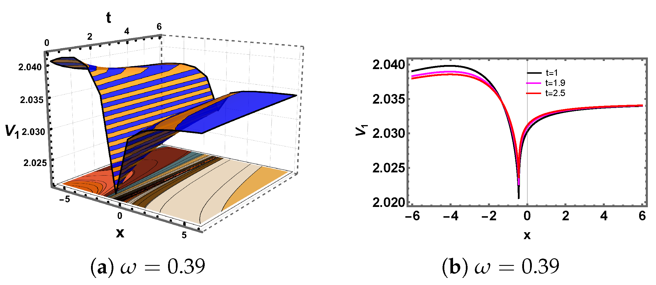
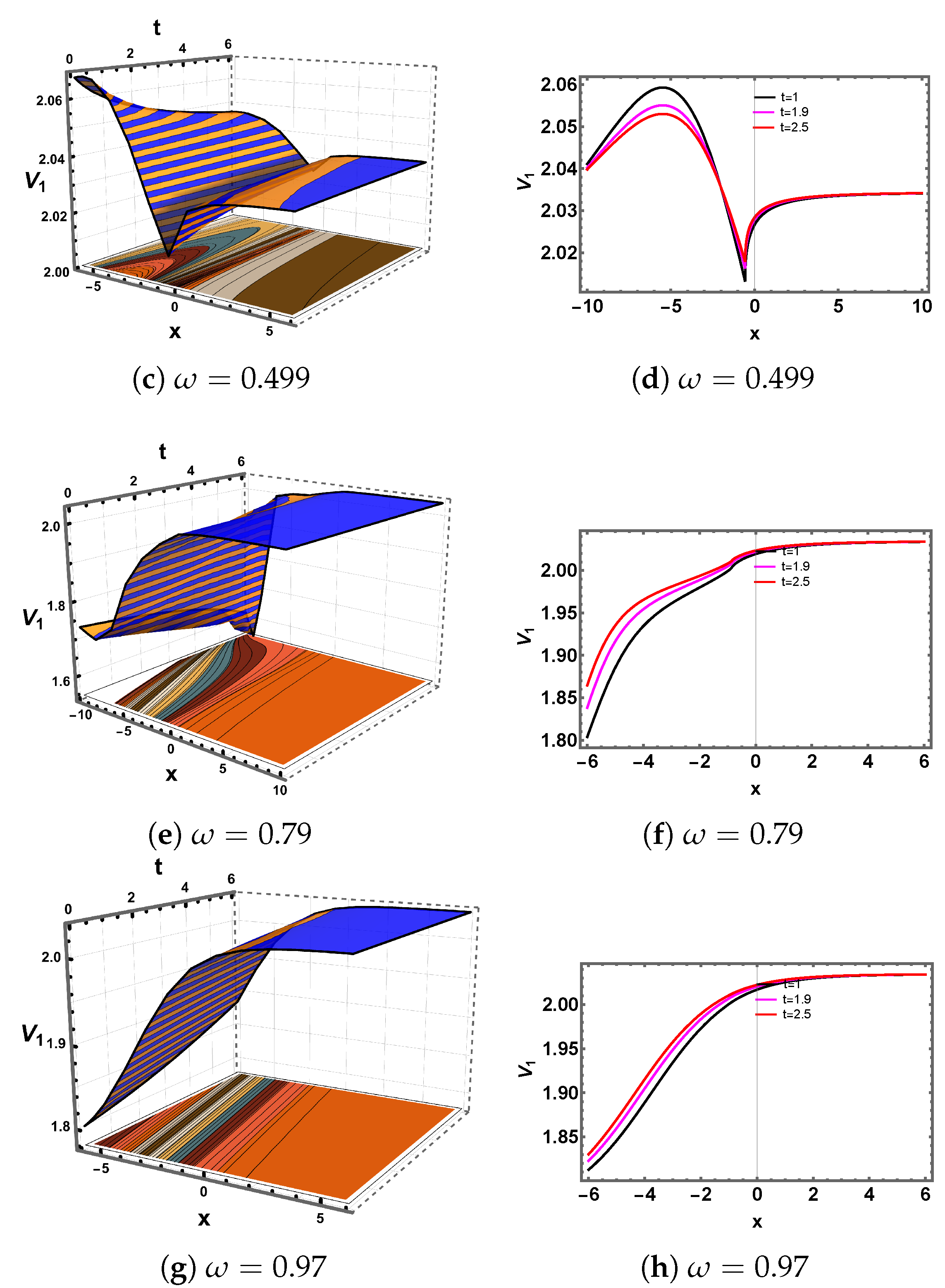
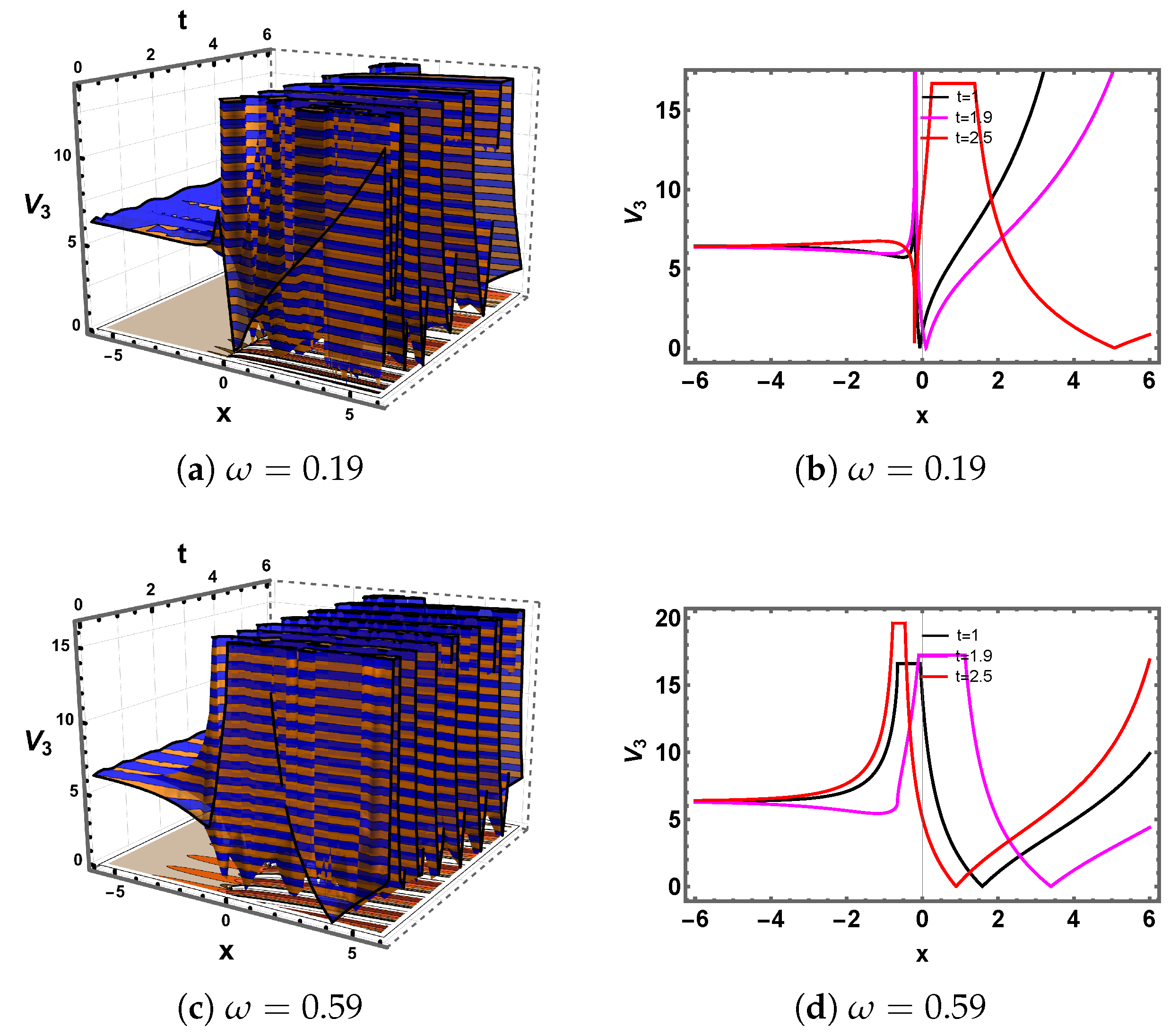
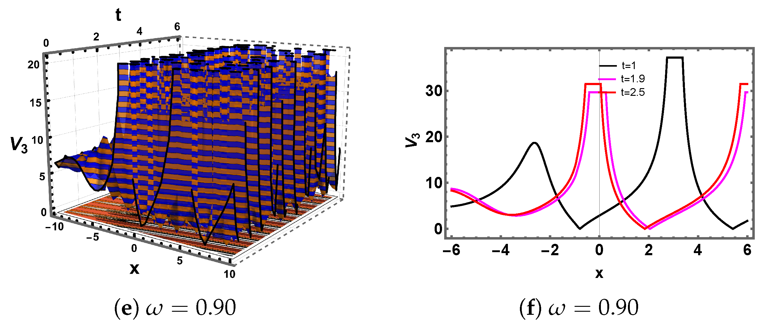
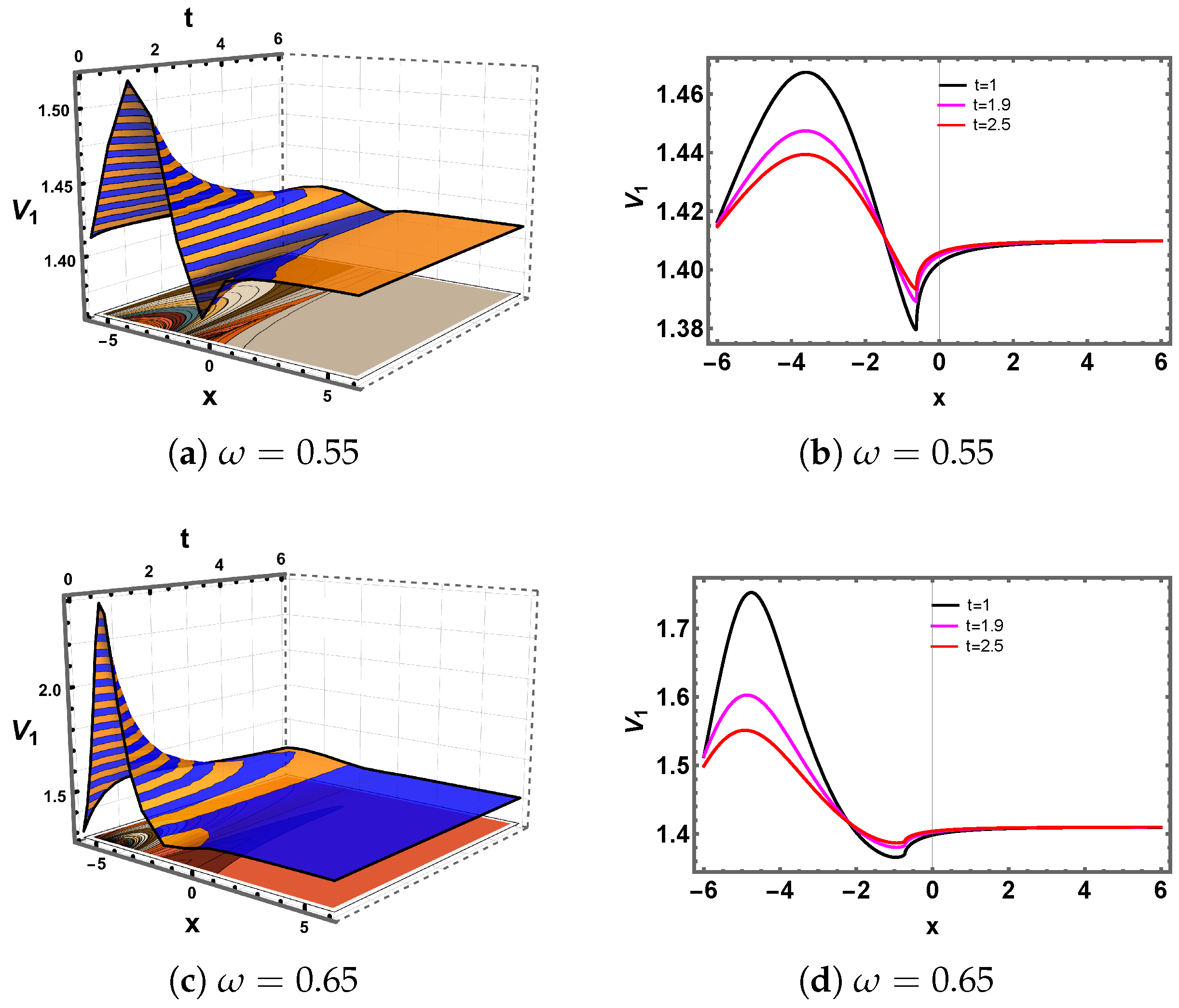
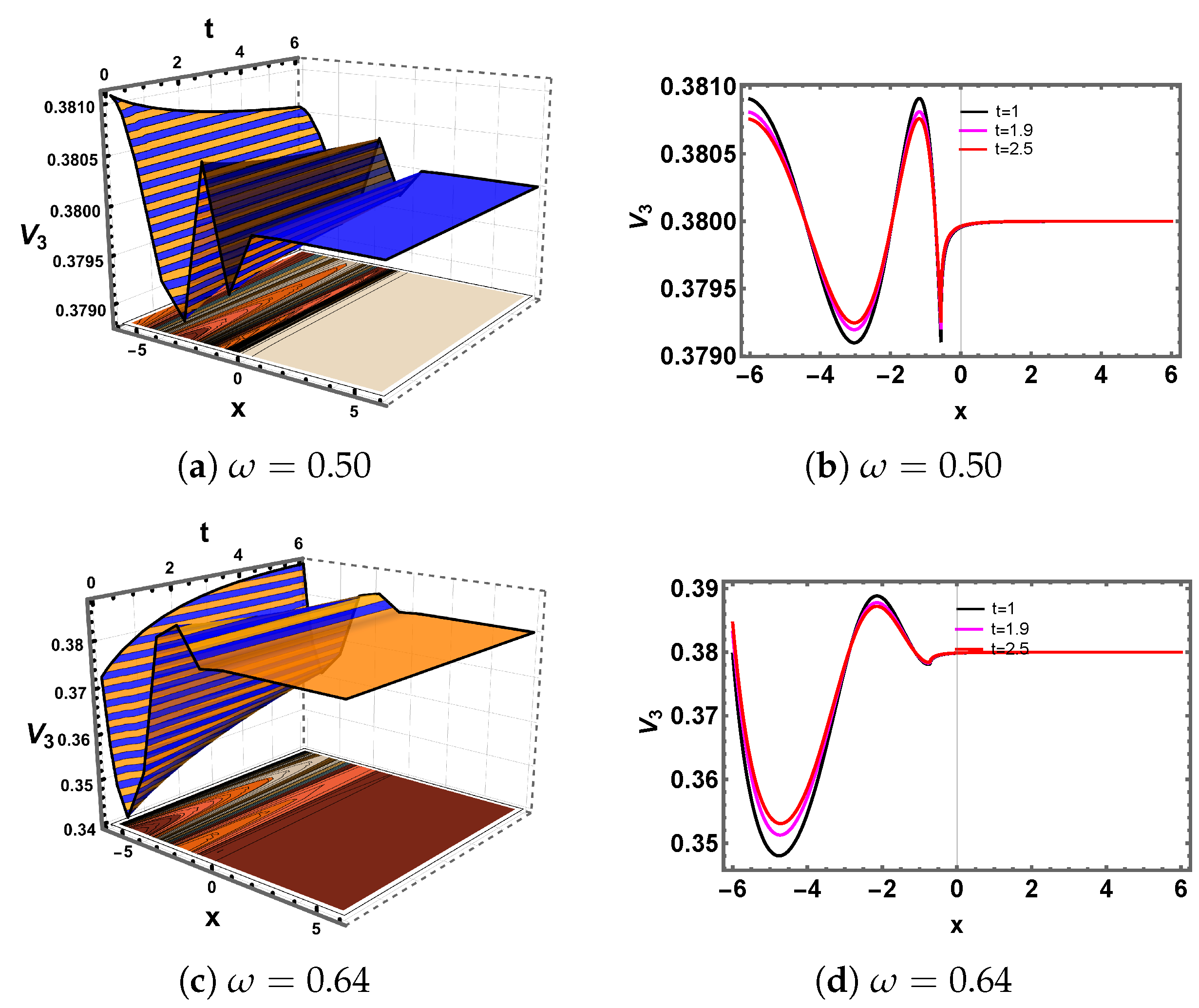
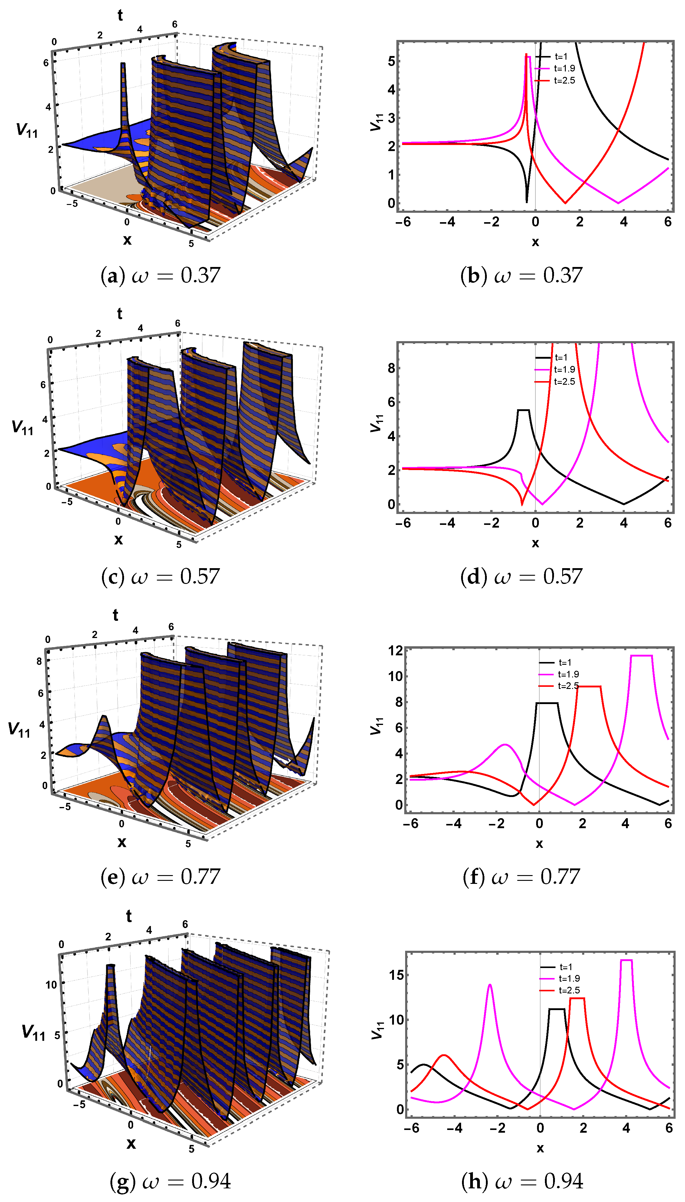
5. Discussion and Graphs

The fractional parameter in mathematical models, particularly in fractional calculus, significantly alters the behavior and properties of graphs representing various functions. By introducing non-integer derivatives or integrals, this parameter allows for the description of complex phenomena with memory and hereditary effects, which classical calculus cannot capture. For instance, in fractional differential equations, varying the fractional parameter can lead to graphs exhibiting slower decay, sharper peaks, or more pronounced tails compared to their integer-order counterparts. This flexibility enables better modeling of anomalous diffusion, viscoelastic materials, and other systems with power-law dynamics. Additionally, the fractional parameter can influence the smoothness and differentiability of the graph, often resulting in fractal-like or irregular features that reflect the underlying non-local interactions. Overall, the fractional parameter enriches the graphical representation of functions, providing deeper insights into systems with long-range dependencies and heterogeneous behavior. A variety of graphs (Figure 1, Figure 2, Figure 3, Figure 4 and Figure 5) were sketched to reflect the impact of fractional parameter $\omega$. It was observed that a slight change in the fractional parameter produced a different behavior of the associated wave.

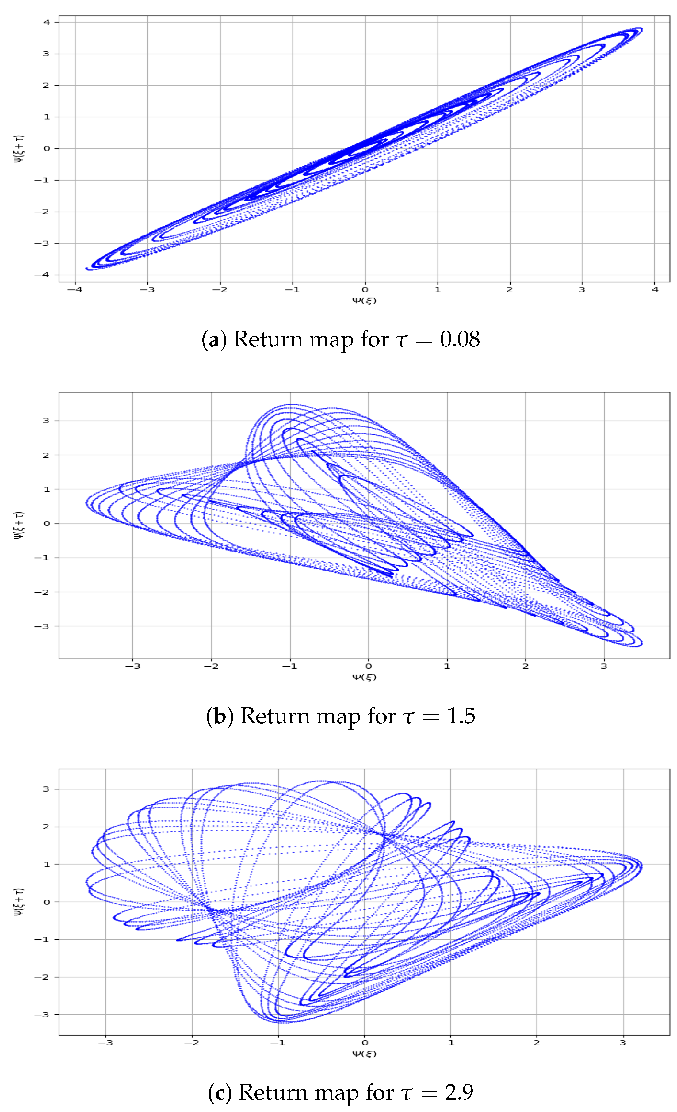
6. Exploring the AKNS Model by Applying a Dynamical System Approach

This section uses perturbed terms to explore the chaotic nature of the studied system. Consider ${\Phi }^{\prime }=\Psi$; we obtain a new relation such that ${k\Psi }^{″}+(4k-\beta )\Psi +6{\Psi }^2=0$. Moreover, on taking ${\Psi }^{\prime }=U$, we get the following dynamical system:

$$\left\{\begin{array}{c}{\displaystyle \frac{d\Psi }{d\xi }}=U,\hfill \\ {\displaystyle \frac{dU}{d\xi }}={\displaystyle \frac{1}{k}}(-(4k-\beta )\Psi -6{\Psi }^2)+\alpha sin\left(X\right),\hfill \\ {\displaystyle \frac{dX}{d\xi }}=n,\hfill \end{array}\right.$$

(41)

where $\alpha sin\left(X\right)$ is the external force, $\alpha$ is the amplitude, and $X=\xi ·n$, where n is the angular frequency. This system models the evolution of the wave amplitude of the state variable $\Psi \left(\xi \right)$ derived from the governing equations, where ${\displaystyle \frac{d\Psi }{d\xi }}=U$ represents its rate of change with respect to spanning time $\xi$. In this, section, we apply the different tools to analyze chaos in system (41).

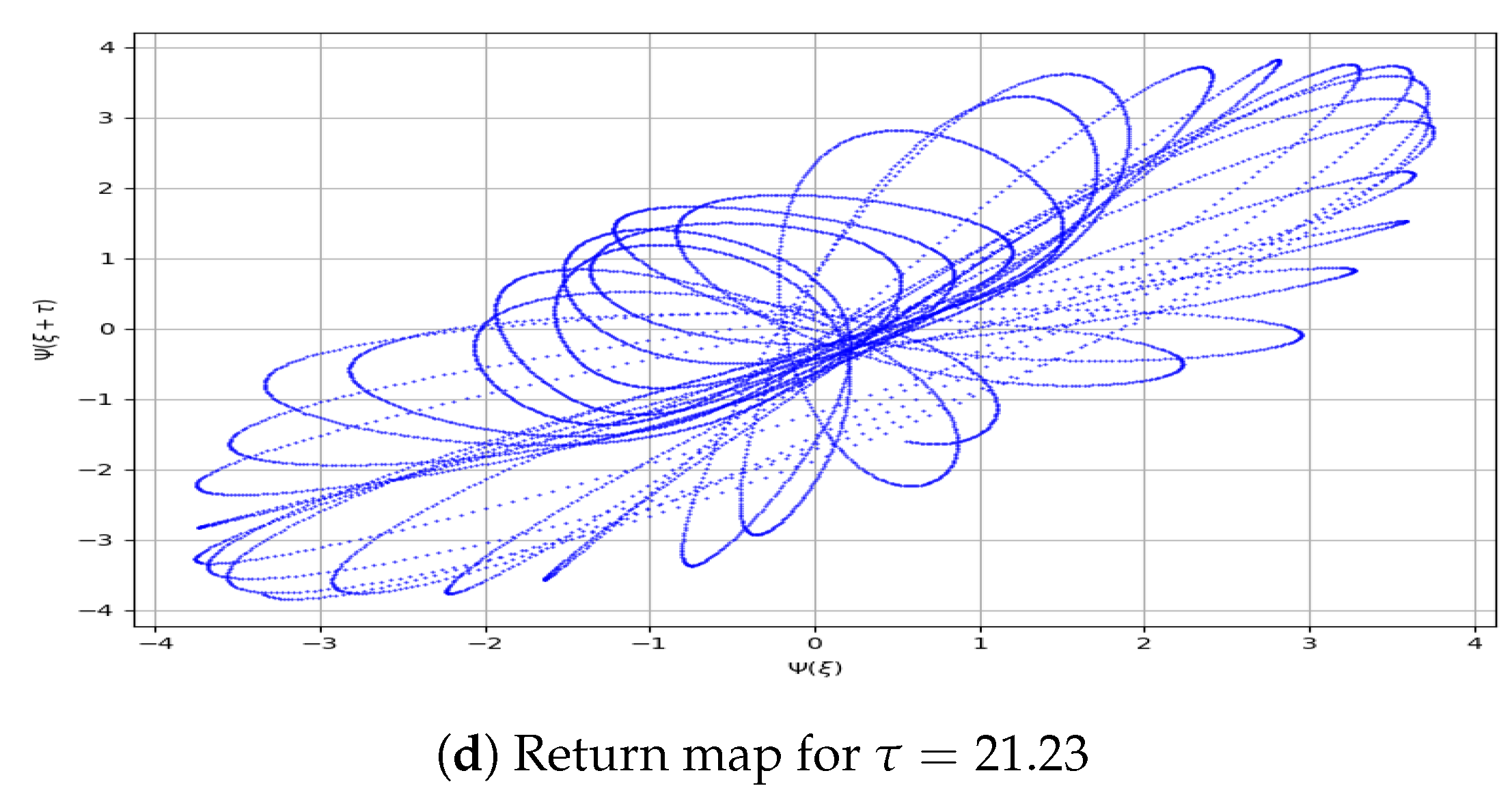
6.1. Return Map

A return map is a simplified representation of a dynamical system’s behavior, constructed by sampling the system’s state at specific intervals, typically when trajectories intersect a predefined surface. By plotting successive intersections, the return map reduces the continuous flow to a discrete mapping, revealing underlying patterns. Its importance lies in detecting chaos: if the return map shows a structured, low-dimensional attractor (e.g., fractal or scattered points with sensitive dependence on initial conditions), it indicates chaotic dynamics. Its applications include analyzing chaotic oscillations in physics (e.g., nonlinear circuits), biology (e.g., neuron firing), and engineering (e.g., rotor dynamics). The return map helps distinguish chaos from noise and quantify stability, periodicity, or bifurcations in complex systems. The return map of the system (41) is presented in Figure 6. $\Psi \left(\xi \right)$ is represented by the horizontal axis and $\Psi (\xi +\tau )$ by the vertical axis, where $\tau$ indicates the small decay.

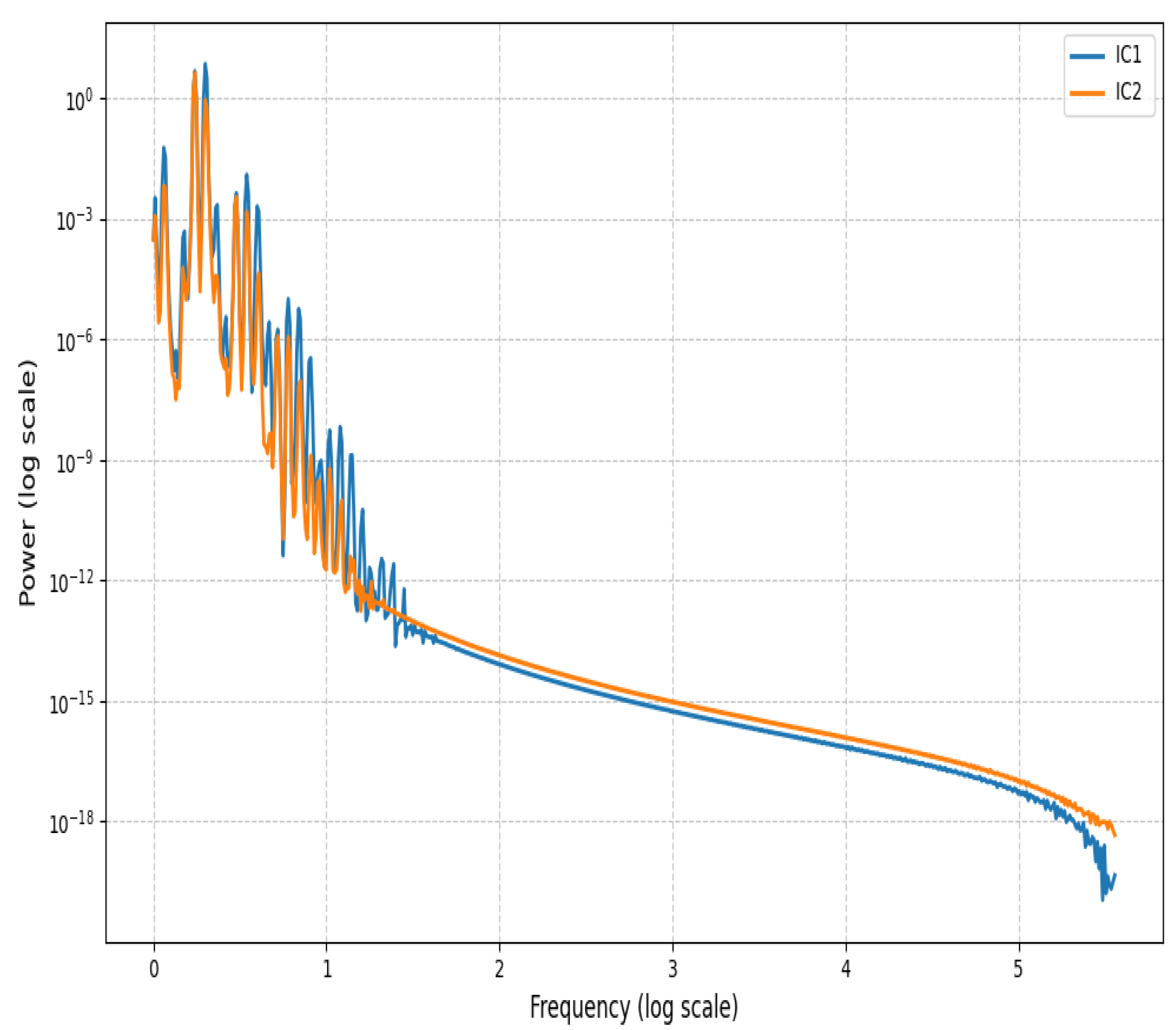
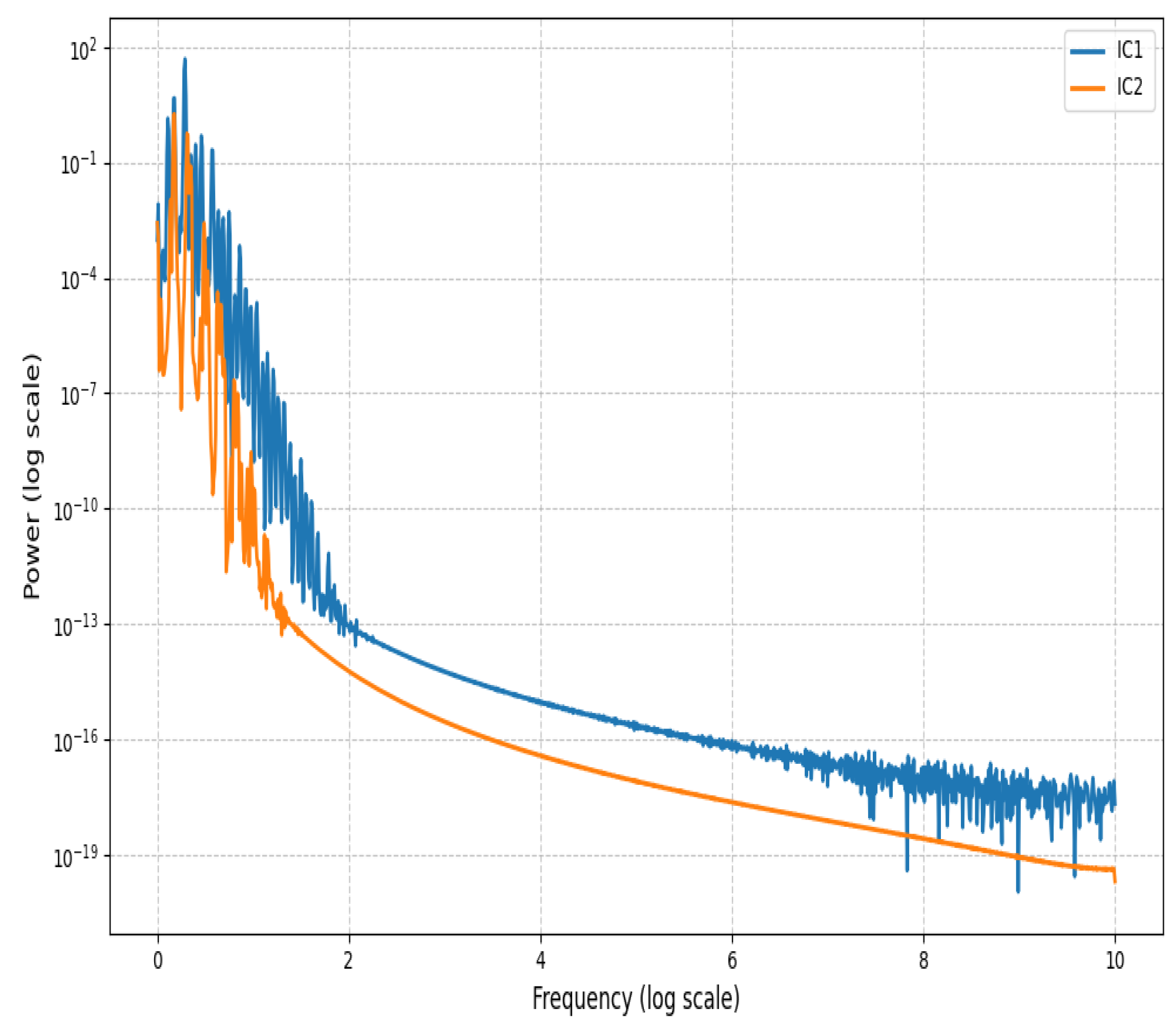
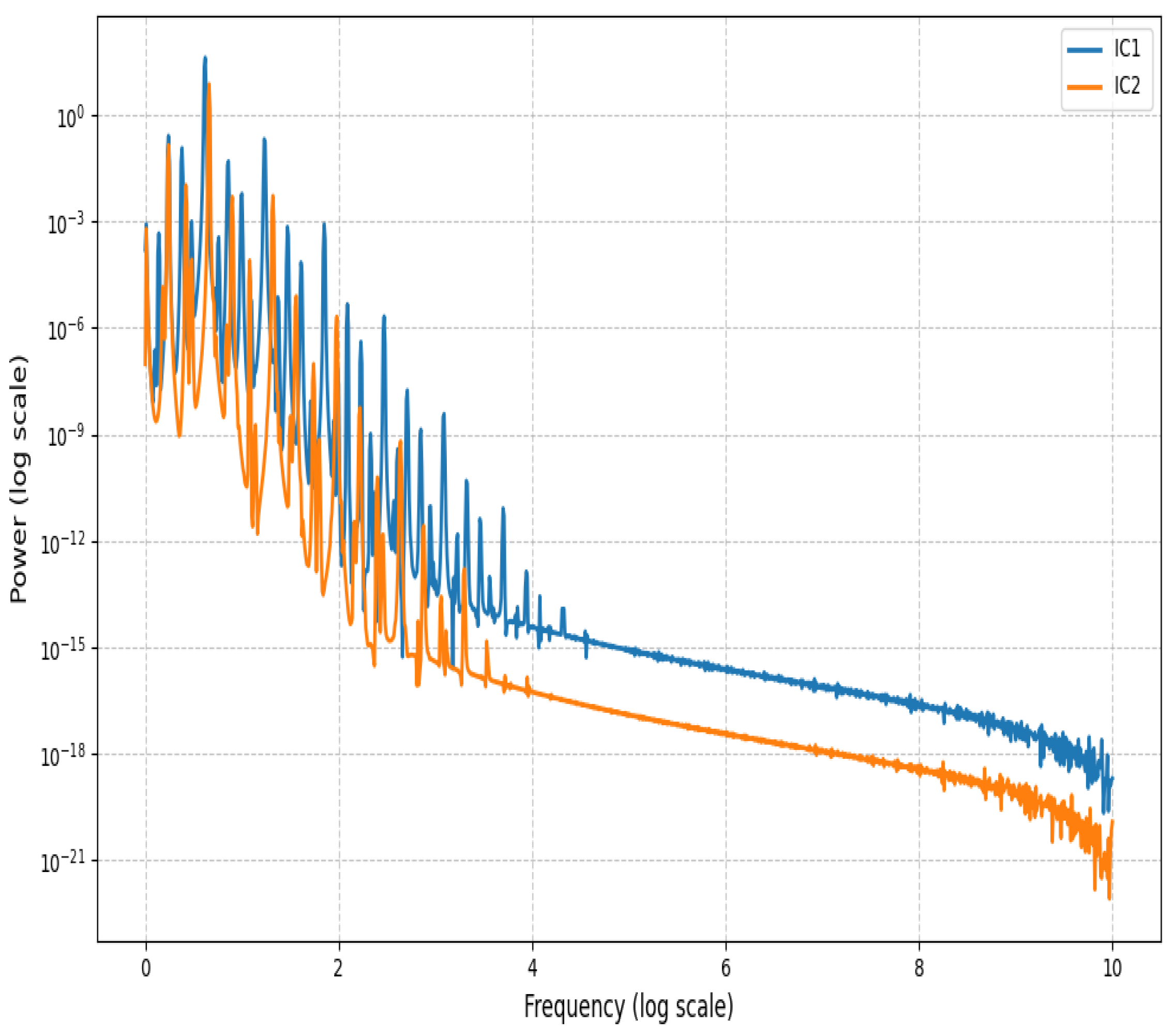
6.2. Power Spectrum

The power spectrum is a fundamental tool in the analysis and characterization of dynamical systems. It quantifies how the energy (or power) of a signal is distributed across different frequencies, revealing its dominant periodicities and underlying frequency structure. By examining the power spectrum, researchers can identify key oscillatory modes, detect chaos (through broadband noise-like spectra), and distinguish between periodic, quasi-periodic, and stochastic behaviors in complex systems. Power spectrum techniques are widely used in fluid dynamics, plasma physics, and optics to analyze complex wave interactions, turbulence, and nonlinear phenomena. In fluid dynamics, power spectra help characterize energy cascades in turbulent flows, identifying inertial ranges and dissipation scales in Kolmogorov-type turbulence. In plasma physics, they reveal electrostatic and electromagnetic wave modes (e.g., Langmuir or Alfvén waves), aiding in the study of instabilities and energy transfer in fusion and space plasmas. In optics, power spectra analyze laser noise, mode dynamics in cavities, and stochastic fluctuations in light–matter interactions, enabling precision measurements and control of coherent light sources. Across these fields, power spectra distinguish deterministic chaos from noise, quantify spectral broadening, and uncover hidden periodicities in nonlinear systems. Different sets of parameters and initial conditions were applied to explore the power spectrum of dynamical system (41) as shown below in Figure 7, Figure 8 and Figure 9. The power spectrum is plotted with frequency (log scale) on the horizontal axis and power (log scale) on the vertical axis. Each graph reveals how vibrational energy distributes across frequencies and how the dynamics evolve under different parameters and initial conditions. At low frequencies, the power spectrum exhibits nearly constant behavior, reflecting large-scale, stable oscillations where the system remains insensitive to minor initial perturbations—evidenced by minimal divergence between curves. A sharp decline in power beyond this range confirms that most of the system’s energy is concentrated in these low-frequency modes.

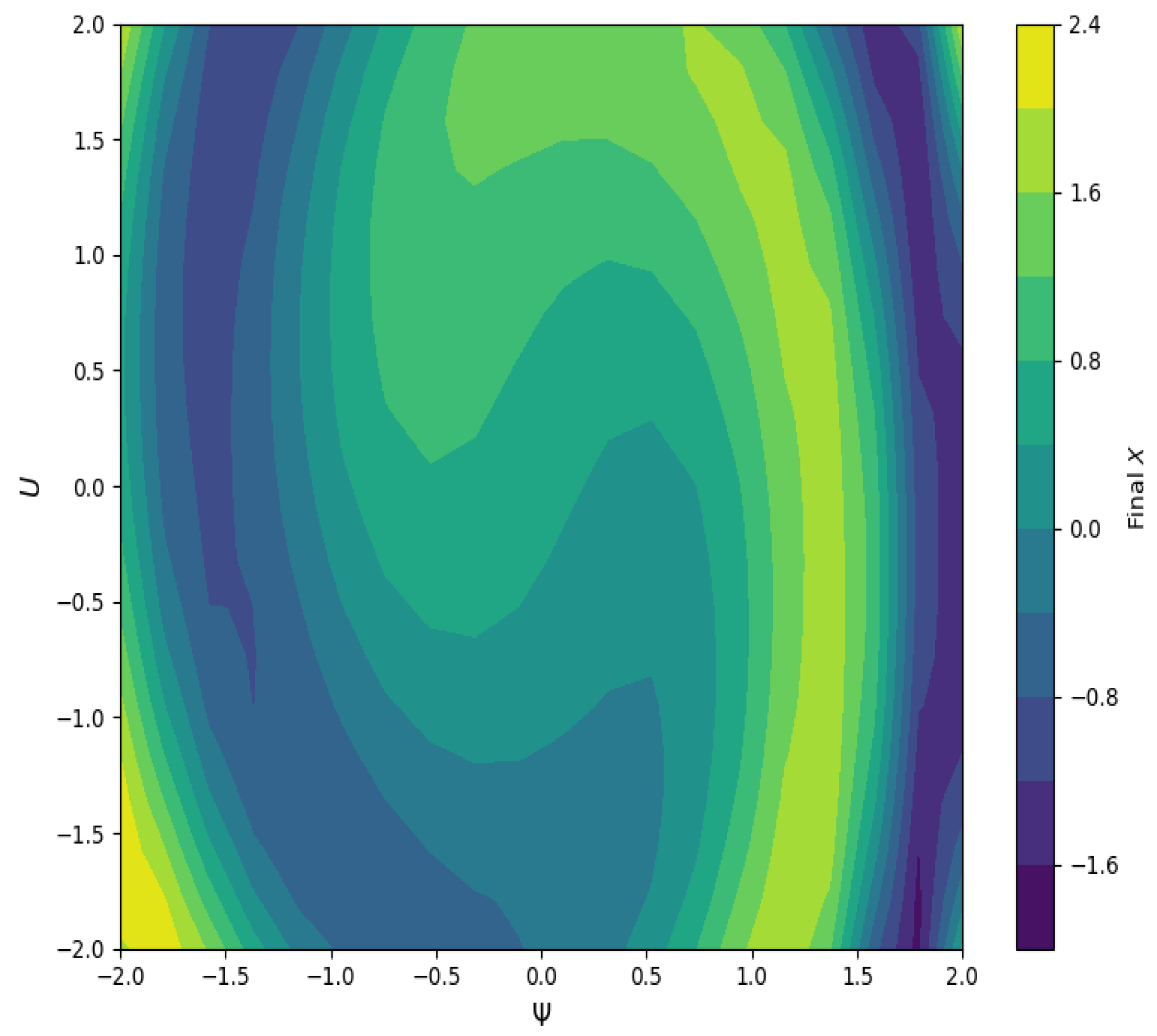
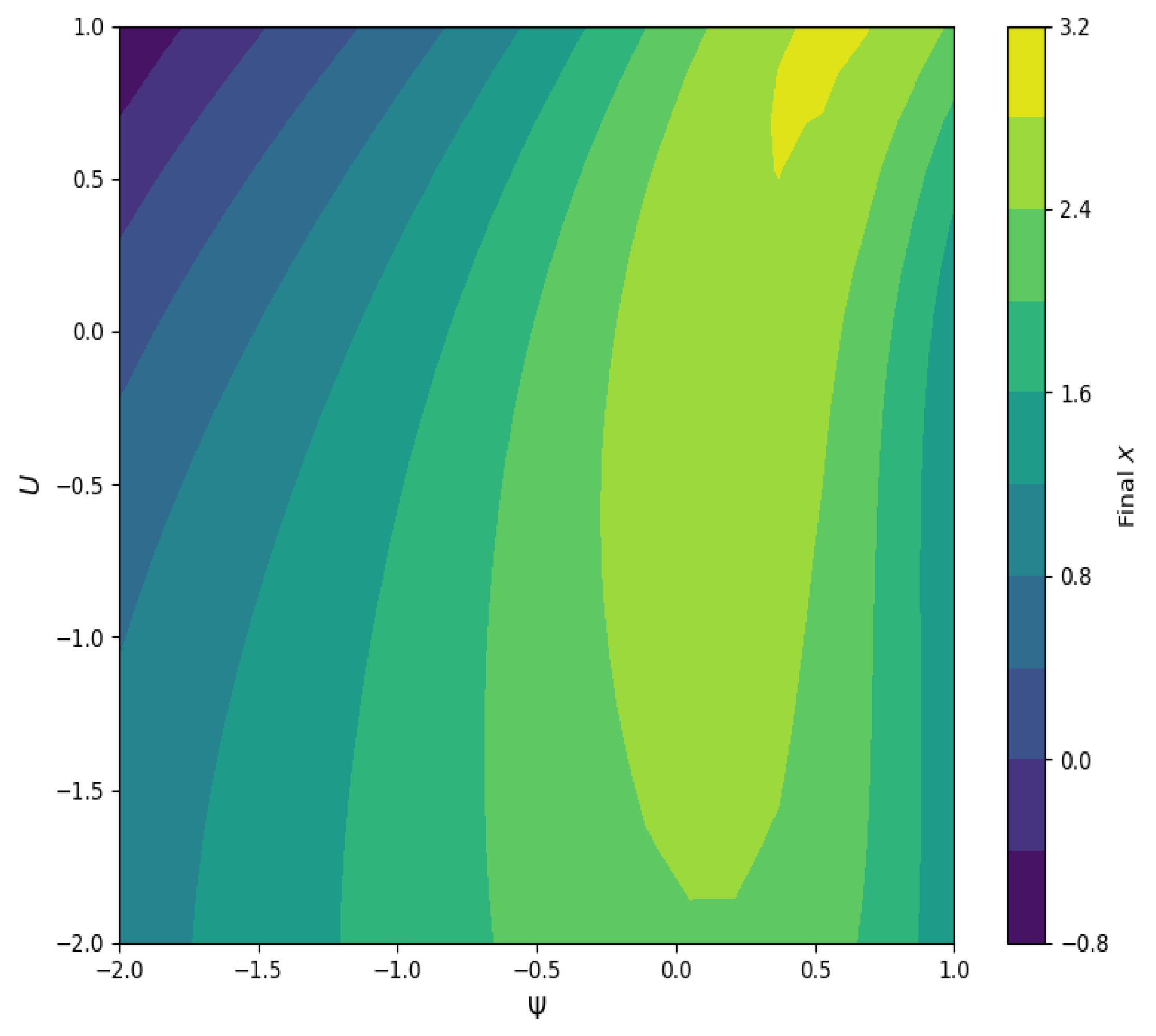
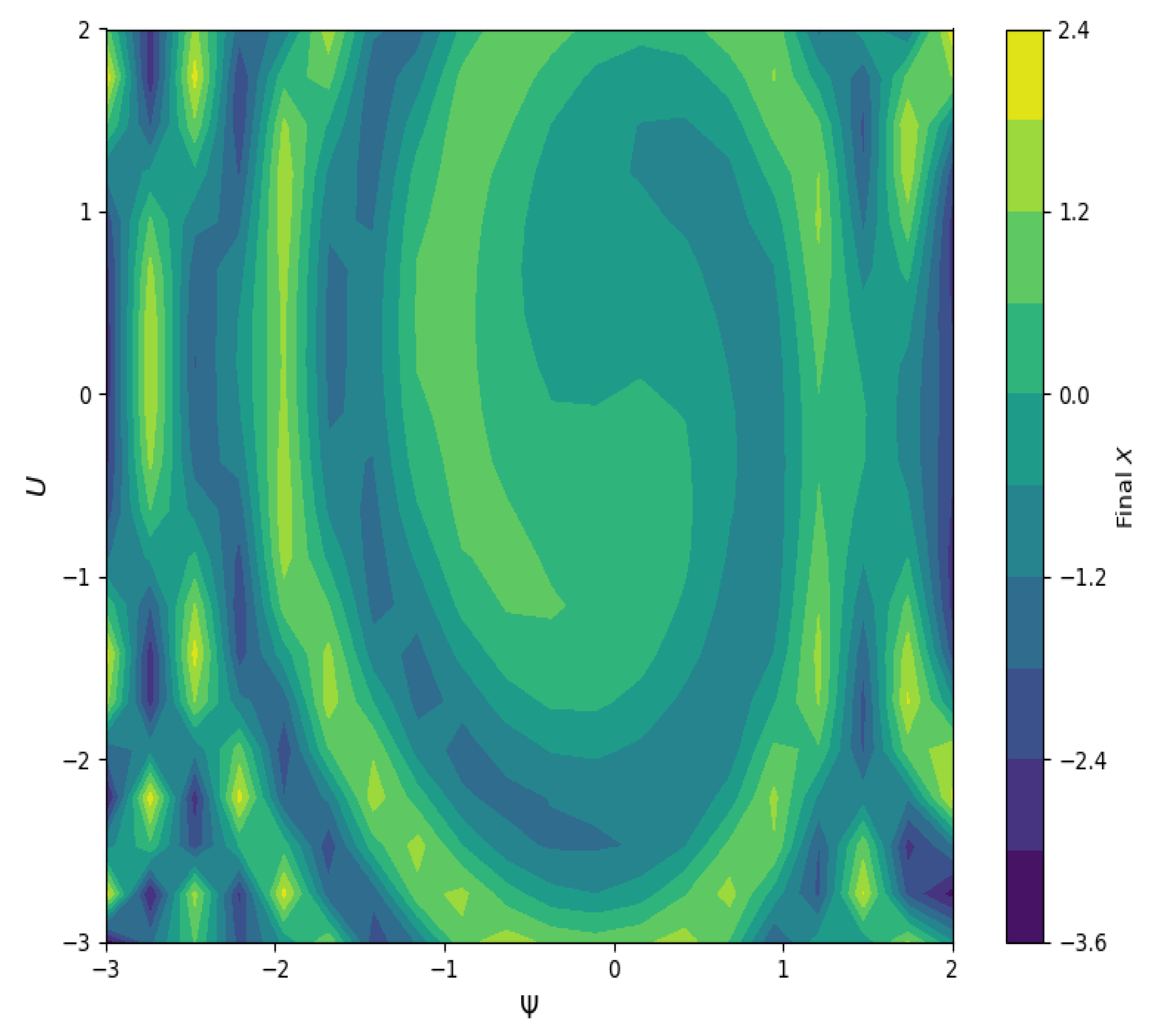
6.3. Basin Attractor

The basin of attraction is a powerful tool for analyzing dynamic systems, defining the set of initial conditions that evolve toward a specific long-term behavior, or attractor. By mapping these basins—often visualized with color-coded regions in 2D systems—we can predict whether a system will stabilize, oscillate, or descend into chaos based on its starting state. This concept is widely applied across disciplines: in physics, it helps model pendulum motion or chaotic fluids like the Lorenz system; in engineering, it ensures stability in control systems and robotics; in biology, it explains neural firing patterns or ecosystem resilience; and in climate science, it reveals thresholds between different environmental regimes. Understanding basins of attraction allows researchers to design robust systems, avoid unstable states, and anticipate how small perturbations might lead to drastically different outcomes—making it essential for studying complexity, multistability, and chaos in real-world phenomena. The graphs of the basin attractor of system (41) are shown in Figure 10, Figure 11 and Figure 12.

7. Concluding Remarks

In conclusion, this study effectively analyzed the nonlinear properties of the fractional AKNS wave model by using analytical approaches, including the generalized projective Riccati equation methodology, nGERFM, and the modified F-expansion technique. The model was used in this context due to its significant scientific and mathematical relevance in defining nonlinear wave phenomena. Due to its inherent nonlinear nature, it encompasses fundamental aspects of wave propagation in fluid dynamics and optical systems, making it a significant subject for research on optical fiber waves. This study successfully derived numerous soliton solutions, including dark, bright, periodic, anti-kink, and kink, therefore offering extensive insights into the system’s dynamics. Visual depictions in Figure 1, Figure 2, Figure 3, Figure 4 and Figure 5 of the selected solutions were included to enhance the analysis of the results. Moreover, chaotic techniques such as the return map, power spectrum analysis, and basin attractors highlighted the system’s sensitivity to initial conditions and the effects of parameters. Figure 6 showed the return map behavior while graphs about the power spectrum were discussed in Figure 7 and Figure 8. Moreover, Figure 10, Figure 11 and Figure 12 represented attractors with different parametric values. These results have a profound influence across several fields, including nonlinear dynamics, mathematical physics, engineering, and applied sciences. Our research clarifies the behavior of solitary waves within physical frameworks, paving the way for novel areas of investigation and prospective applications.

References

- Demirbilek, U.; Nadeem, M.; Çelik, F.M.; Bulut, H.; Şenol, M. Generalized extended (2+1)-dimensional Kadomtsev–Petviashvili equation in fluid dynamics: Analytical solutions. Nonlinear Dyn. 2024, 112, 13393–13408. [Google Scholar] [CrossRef]
- Ecke, R.E. Chaos, patterns, coherent structures, and turbulence: Reflections on nonlinear science. Chaos Interdiscip. J. Nonlinear Sci. 2015, 25, 097605. [Google Scholar] [CrossRef] [PubMed]
- Alshammari, S.; Al-Sawalha, M.M.; Shah, R. Approximate analytical methods for a fractional-order nonlinear system of Jaulent–Miodek equation with energy-dependent Schrödinger potential. Fractal Fract. 2023, 7, 140. [Google Scholar] [CrossRef]
- Nicolis, G. Introduction to Nonlinear Science; Cambridge University Press: Cambridge, UK, 1995. [Google Scholar]
- Remond-Tiedrez, A. Nonlinear Partial Differential Equations in Fluid Dynamics: Interfaces, Microstructure, and Stability. Ph.D. Thesis, Carnegie Mellon University, Pittsburgh, PA, USA, 2020. [Google Scholar]
- Roubíček, T. Nonlinear Partial Differential Equations with Applications; Springer Science & Business Media: Basel, Switzerland, 2013. [Google Scholar]
- Russell, J.S. Report on Waves: Made to the Meetings of the British Association in 1845; John Murray: London, UK, 1845. [Google Scholar]
- Wadati, M. The modified Korteweg–de Vries equation. J. Phys. Soc. Jpn. 1973, 34, 1289–1296. [Google Scholar] [CrossRef]
- Muhammad, J.; Bilal, M.; Rehman, S.U.; Nasreen, N.; Younas, U. Analyzing the decoupled nonlinear Schrödinger equation: Fractional optical wave patterns in the dual-core fibers. J. Opt. 2024, 1–12. [Google Scholar] [CrossRef]
- Murad, M.A.S.; Mahmood, S.S.; Emadifar, H.; Mohammed, W.W.; Ahmed, K.K. Optical soliton solution for dual-mode time-fractional nonlinear Schrödinger equation by generalized exponential rational function method. Results Eng. 2025, 27, 105591. [Google Scholar] [CrossRef]
- Zayed, E.; Alngar, M.; Shohib, R.; Biswas, A.; Yildirim, Y.; Moraru, L.; Georgescu, P.; Iticescu, C.; Asiri, A. Highly dispersive solitons in optical couplers with metamaterials having Kerr law of nonlinear refractive index. Ukr. J. Phys. Opt. 2024, 25, 01001–01019. [Google Scholar] [CrossRef]
- Younas, U.; Muhammad, J.; Murad, M.A.S.; Almutairi, D.; Khan, A.; Abdeljawad, T. Investigating the truncated fractional telegraph equation in engineering: Solitary wave solutions. Results Eng. 2025, 25, 104489. [Google Scholar] [CrossRef]
- Serge, D.Y.; Justin, M.; Betchewe, G.; Crepin, K.T. Optical chirped soliton in metamaterials. Nonlinear Dyn. 2017, 90, 13–18. [Google Scholar] [CrossRef]
- Duan, J.S.; Rach, R.; Baleanu, D.; Wazwaz, A.M. A review of the Adomian decomposition method and its applications to fractional differential equations. Commun. Fract. Calc. 2012, 3, 73–99. [Google Scholar]
- Younas, U.; Muhammad, J.; Ali, Q.; Sediqmal, M.; Kedzia, K.; Jan, A.Z. On the study of solitary wave dynamics and interaction phenomena in the ultrasound imaging modelled by the fractional nonlinear system. Sci. Rep. 2024, 14, 26080. [Google Scholar] [CrossRef]
- Raza, N.; Rani, B.; Chahlaoui, Y.; Shah, N.A. A variety of new rogue wave patterns for three coupled nonlinear Maccari’s models in complex form. Nonlinear Dyn. 2023, 111, 18419–18437. [Google Scholar] [CrossRef]
- Raza, N.; Salman, F.; Butt, A.R.; Gandarias, M.L. Soliton solutions and qualitative analysis concerning to the generalized q-deformed Sinh–Gordon equation. Commun. Nonlinear Sci. Numer. Simul. 2023, 116, 106824. [Google Scholar] [CrossRef]
- Muhammad, J.; Younas, U.; Almutairi, D.; Khan, A.; Abdeljawad, T. Optical wave features and sensitivity analysis of a coupled fractional integrable system. Results Phys. 2025, 68, 108060. [Google Scholar] [CrossRef]
- Zhu, S.-D. The generalizing Riccati equation mapping method in non-linear evolution equation: Application to (2+1)-dimensional Boiti–Leon–Pempinelle equation. Chaos Solitons Fractals 2008, 37, 1335–1342. [Google Scholar] [CrossRef]
- Hosseini, K.; Samadani, F.; Kumar, D.; Faridi, M. New optical solitons of cubic-quartic nonlinear Schrödinger equation. Optik 2018, 157, 1101–1105. [Google Scholar] [CrossRef]
- Mañas, M. Darboux transformations for the nonlinear Schrödinger equations. J. Phys. A Math. Gen. 1996, 29, 7721–7737. [Google Scholar] [CrossRef]
- Gu, Y.; Chen, B.; Ye, F.; Aminakbari, N. Soliton solutions of nonlinear Schrödinger equation with the variable coefficients under the influence of Woods–Saxon potential. Results Phys. 2022, 42, 105979. [Google Scholar] [CrossRef]
- Han, T.; Li, Z.; Li, C. Stationary optical solitons and exact solutions for generalized nonlinear Schrödinger equation with nonlinear chromatic dispersion and quintuple power-law of refractive index in optical fibers. Phys. A Stat. Mech. Appl. 2023, 615, 128599. [Google Scholar] [CrossRef]
- Muhammad, J.; Ali, Q.; Younas, U. On the analysis of optical pulses to the fractional extended nonlinear system with mechanism of third-order dispersion arising in fiber optics. Opt. Quantum Electron. 2024, 56, 1168. [Google Scholar] [CrossRef]
- Ullah, M.S.; Ali, M.Z.; Roshid, H.-O. And diverse chaos-detecting tools for the DSKP model. Sci. Rep. 2025, 15, 13658. [Google Scholar] [CrossRef]
- Vivas-Cortez, M.; Sadaf, M.; Arshed, S.; Rehan, K.; Akram, G.; Saeed, K.; Shmarev, S. Extraction of Optical Solitons for Conformable Perturbed Gerdjikov–Ivanov Equation via Two Integrating Techniques. Adv. Math. Phys. 2024, 2024, 5936389. [Google Scholar] [CrossRef]
- Ali, K.K.; Yokus, A.; Seadawy, A.R.; Yilmazer, R. The ion sound and Langmuir waves dynamical system via computational modified generalized exponential rational function. Chaos Solitons Fractals 2022, 161, 112381. [Google Scholar] [CrossRef]
- Ozdemir, N.; Secer, A.; Ozisik, M.; Bayram, M. Optical soliton solutions of the nonlinear Schrödinger equation in the presence of chromatic dispersion with cubic-quintic-septic-nonic nonlinearities. Phys. Scr. 2023, 98, 115223. [Google Scholar] [CrossRef]
- Atangana, A.; Goufo, E.F.D.; Jafari, H. Extension of matched asymptotic method to fractional boundary layers problems. Math. Probl. Eng. 2014, 2014, 107535. [Google Scholar] [CrossRef]
- Atangana, A.; Baleanu, D. New fractional derivatives with nonlocal and non-singular kernel: Theory and application to heat transfer model. Therm. Sci. 2016, 20, 763–769. [Google Scholar] [CrossRef]
- Khurshaid, A.; Khurshaid, H. Comparative Analysis and Definitions of Fractional Derivatives. J. Biomed. Res. Environ. Sci. 2023, 4, 1684–1688. [Google Scholar] [CrossRef]
- Atangana, A.; Baleanu, D.; Alsaedi, A. Analysis of time-fractional Hunter–Saxton equation: A model of nematic liquid crystal. Open Phys. 2016, 14, 145–149. [Google Scholar] [CrossRef]
- Sahoo, S.; Ray, S.S. Invariant analysis with conservation law of time fractional coupled Ablowitz–Kaup–Newell–Segur equations in water waves. Waves Random Complex Media 2020, 30, 530–543. [Google Scholar] [CrossRef]
- Sun, J. Variational principle and solitary wave of the fractal fourth-order nonlinear Ablowitz–Kaup–Newell–Segur water wave model. Fractals 2023, 31, 2350036. [Google Scholar] [CrossRef]
- Thadee, W.; Chankaew, A.; Phoosree, S. Effects of wave solutions on shallow-water equation, optical-fibre equation and electric-circuit equation. Maejo Int. J. Sci. Technol. 2022, 16, 262–274. [Google Scholar]
- Eskitaşçıoğlu, E.İ.; Aktaş, M.B.; Baskonus, H.M. New Complex and Hyperbolic Forms for Ablowitz–Kaup–Newell–Segur Wave Equation with Fourth Order. Appl. Math. Nonlinear Sci. 2019, 4, 93–100. [Google Scholar] [CrossRef]
- Zafar, A.; Saboor, A.; Inc, M.; Ashraf, M.; Ahmad, S. New fractional solutions for the Clannish Random Walker’s Parabolic equation and the Ablowitz–Kaup–Newell–Segur equation. Opt. Quantum Electron. 2024, 56, 581. [Google Scholar] [CrossRef]
- Dusunceli, F. New exact solutions for Ablowitz–Kaup–Newell–Segur water wave Equation. Sigma 2019, 10, 171–177. [Google Scholar]
Disclaimer/Publisher’s Note: The statements, opinions and data contained in all publications are solely those of the individual author(s) and contributor(s) and not of MDPI and/or the editor(s). MDPI and/or the editor(s) disclaim responsibility for any injury to people or property resulting from any ideas, methods, instructions or products referred to in the content. |
© 2025 by the authors. Licensee MDPI, Basel, Switzerland. This article is an open access article distributed under the terms and conditions of the Creative Commons Attribution (CC BY) license (https://creativecommons.org/licenses/by/4.0/).
Share and Cite
Muhammad, J.; Tedjani, A.H.; Hussain, E.; Younas, U. Investigating Chaotic Techniques and Wave Profiles with Parametric Effects in a Fourth-Order Nonlinear Fractional Dynamical Equation. Fractal Fract. 2025, 9, 487. https://doi.org/10.3390/fractalfract9080487
Muhammad J, Tedjani AH, Hussain E, Younas U. Investigating Chaotic Techniques and Wave Profiles with Parametric Effects in a Fourth-Order Nonlinear Fractional Dynamical Equation. Fractal and Fractional. 2025; 9(8):487. https://doi.org/10.3390/fractalfract9080487
Chicago/Turabian StyleMuhammad, Jan, Ali H. Tedjani, Ejaz Hussain, and Usman Younas. 2025. "Investigating Chaotic Techniques and Wave Profiles with Parametric Effects in a Fourth-Order Nonlinear Fractional Dynamical Equation" Fractal and Fractional 9, no. 8: 487. https://doi.org/10.3390/fractalfract9080487
APA StyleMuhammad, J., Tedjani, A. H., Hussain, E., & Younas, U. (2025). Investigating Chaotic Techniques and Wave Profiles with Parametric Effects in a Fourth-Order Nonlinear Fractional Dynamical Equation. Fractal and Fractional, 9(8), 487. https://doi.org/10.3390/fractalfract9080487