
Evaluating the Fractal Pattern of the Von Koch Island Using Richardson’s Method


Abstract
1. Introduction
1.1. About Fractal Geometry
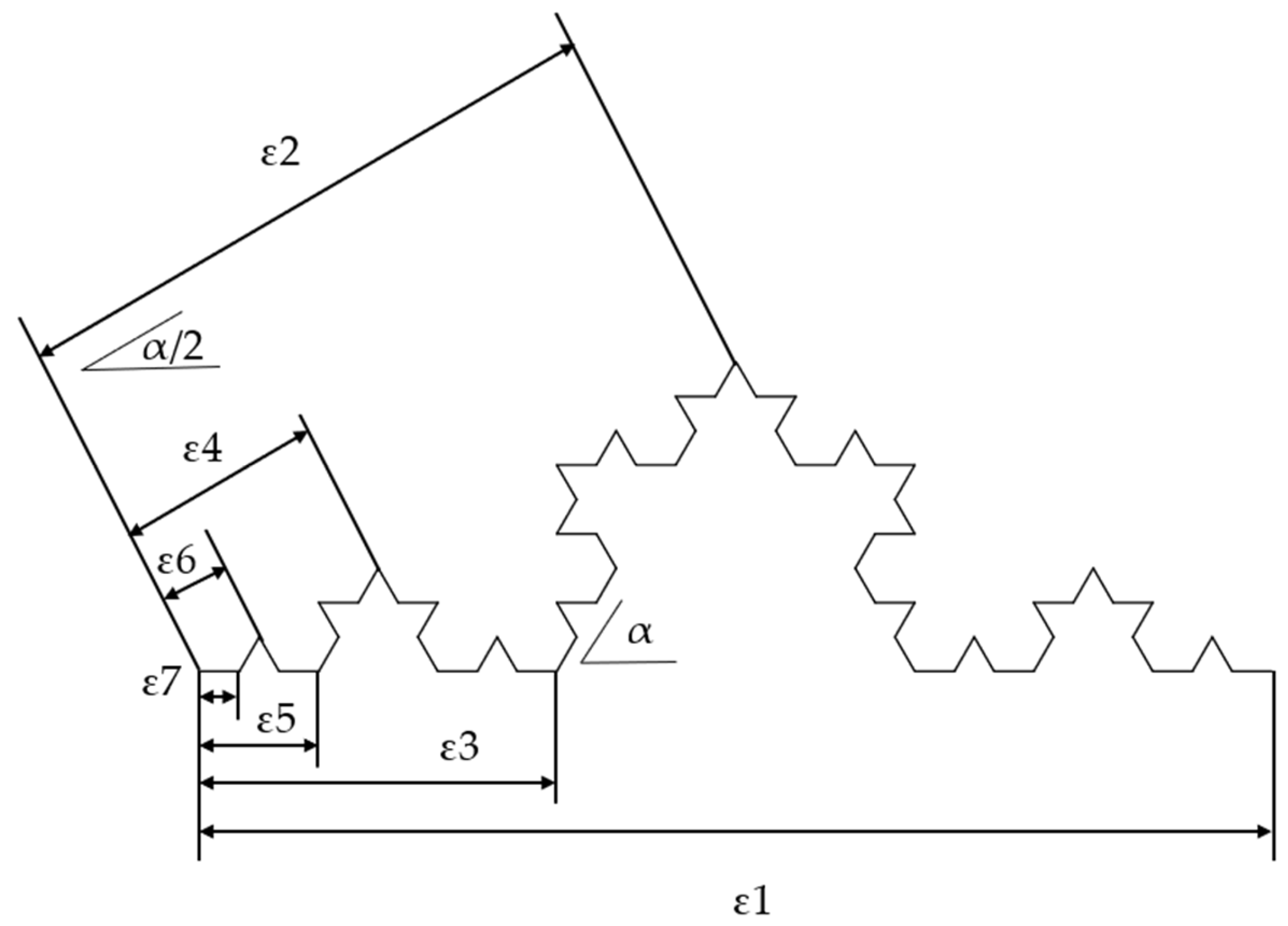
1.2. The Definition of the Koch Curve
2. Materials and Methods
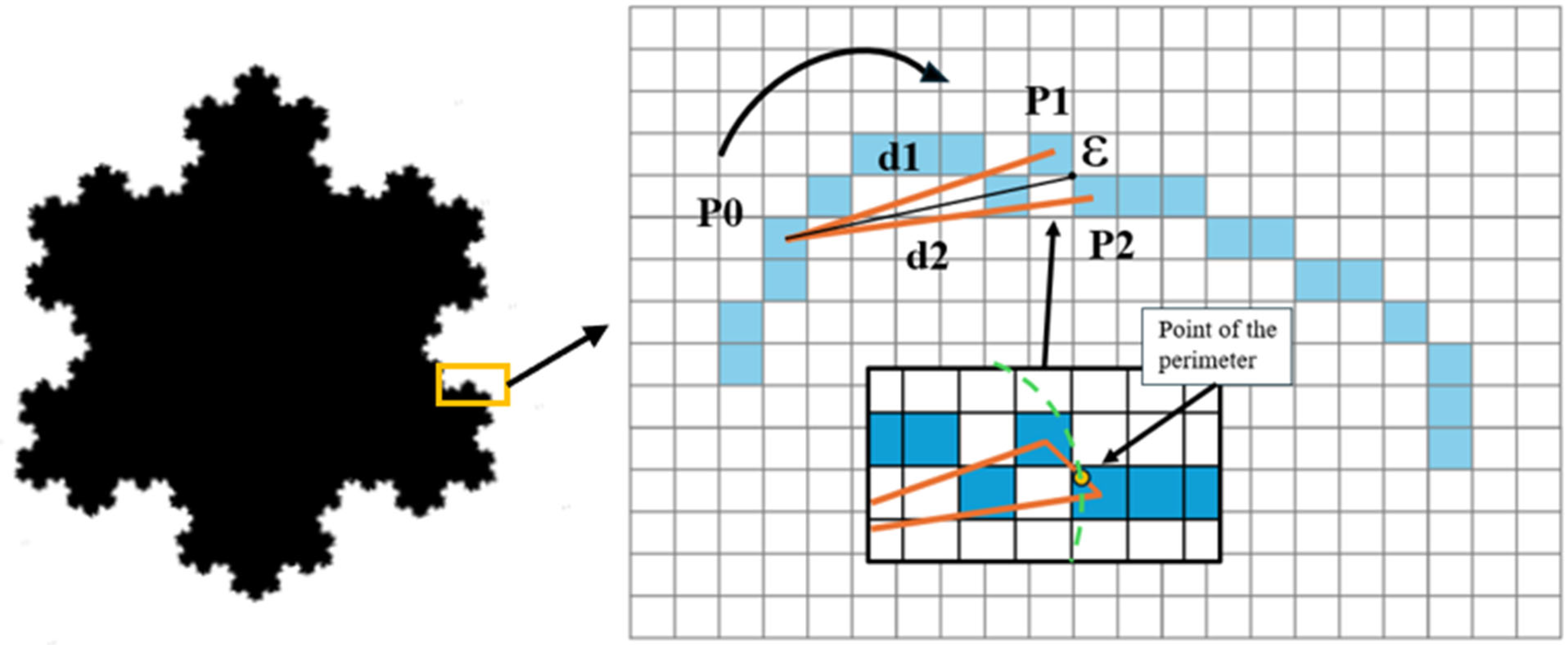
2.1. Richardson’s Method and Perimeter-Based Fractal Dimension Estimation
2.2. Computer Software and Statistical Estimation
- Images as large as possible are needed to analyze the properties of the fractal curves. The application we developed allows creating images without size limits (except for the RAM memory of the computer).
- Some of the fractal’s properties require a special implementation that will not be found in the usual software.
- As reported in the literature, some results could depend on the implementation such as error discretization or statistical methods. No doubt must remain about numerical implementation to analyze the efficiency of Richardson’s method, and therefore all parts of the software must be controlled without any assumptions about the implementation or the algorithm used.
2.3. Fractal Curve Generation Software (FCGS)
2.4. Fractal Analysis System Software
2.5. Statistical Estimation of the Fractal Dimension
- The yardstick linear variation (YLV): , where is the linear increment,
- The yardstick geometrical variation (YGV): , where q is a geometrical increment.
- It can be proved than , then the YGV method is always the more appropriate to calculate ∆ with a good accuracy.
- Using the YLV method, the experimental weight is not uniform and ∆ is more influenced by the estimated perimeter for large yardstick rather than for smaller one. The higher , the higher the perimeter for large yardsticks.
- As we shall see in the next paragraph, discretization errors can lead to an erroneous measurement of the perimeter for large yardsticks, consequently the YLV method could overestimate or underestimate the fractal dimension of the image.
3. Curve Analyses
3.1. Analyses on the Von Koch Flake
- A 1.2 fractal dimension Von Koch flake with α = 54° instead of 60° is computed with a resolution of 2048 × 2048 pixels (we use this dimension on purpose to compare with the Von Koch flake since it is impossible to construct a Stochastic flake defined in Section 4 without recovering). Seven iterations are carried out to construct the flake.
- The origin of the yardstick is chosen at random.
- The fractal dimension is calculated by the YGV method and the perimeter’s length is computed by Method 4 (floating number of yardstick).
- The starting point for the first yardstick is chosen at random.
- A second iteration is carried out taking the previous origin + 1 pixel.
- The operation is repeated for δ varying from 1 to 500 pixels.
- Then the following statistics are built:
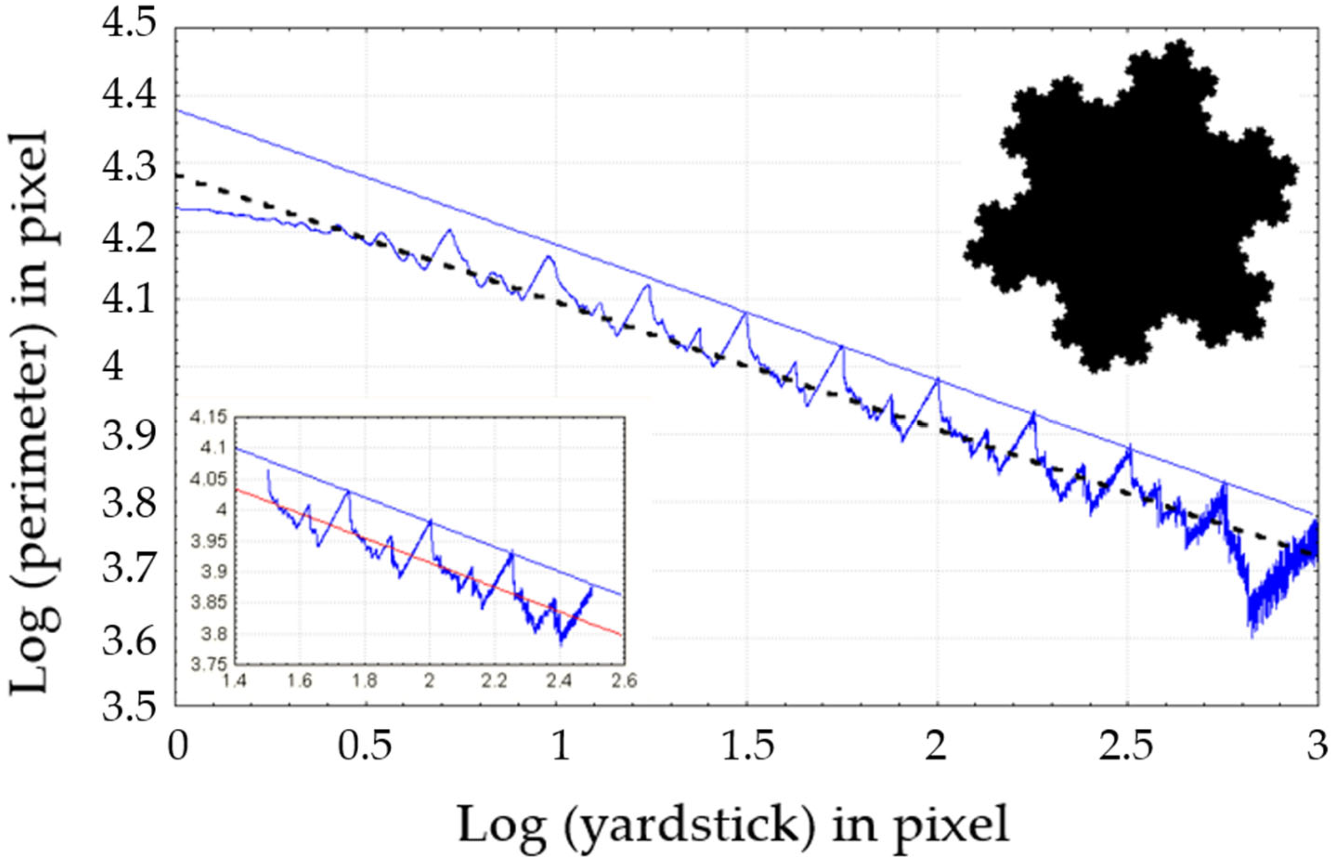
- The computed perimeter is the mean of these 500 perimeters.
- The computed perimeter is the maximum of these 500 perimeters.
- The standard deviation is computed.
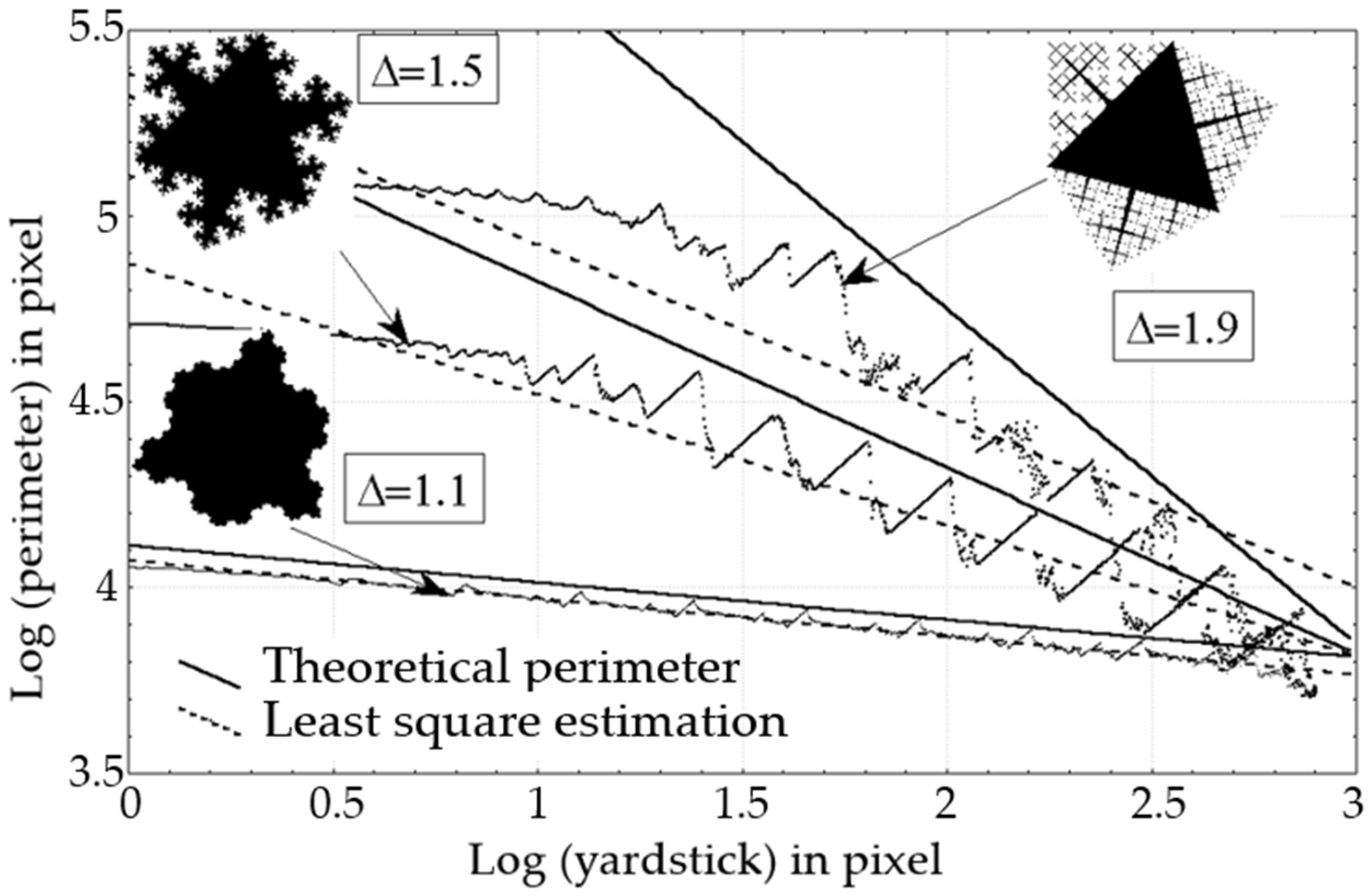
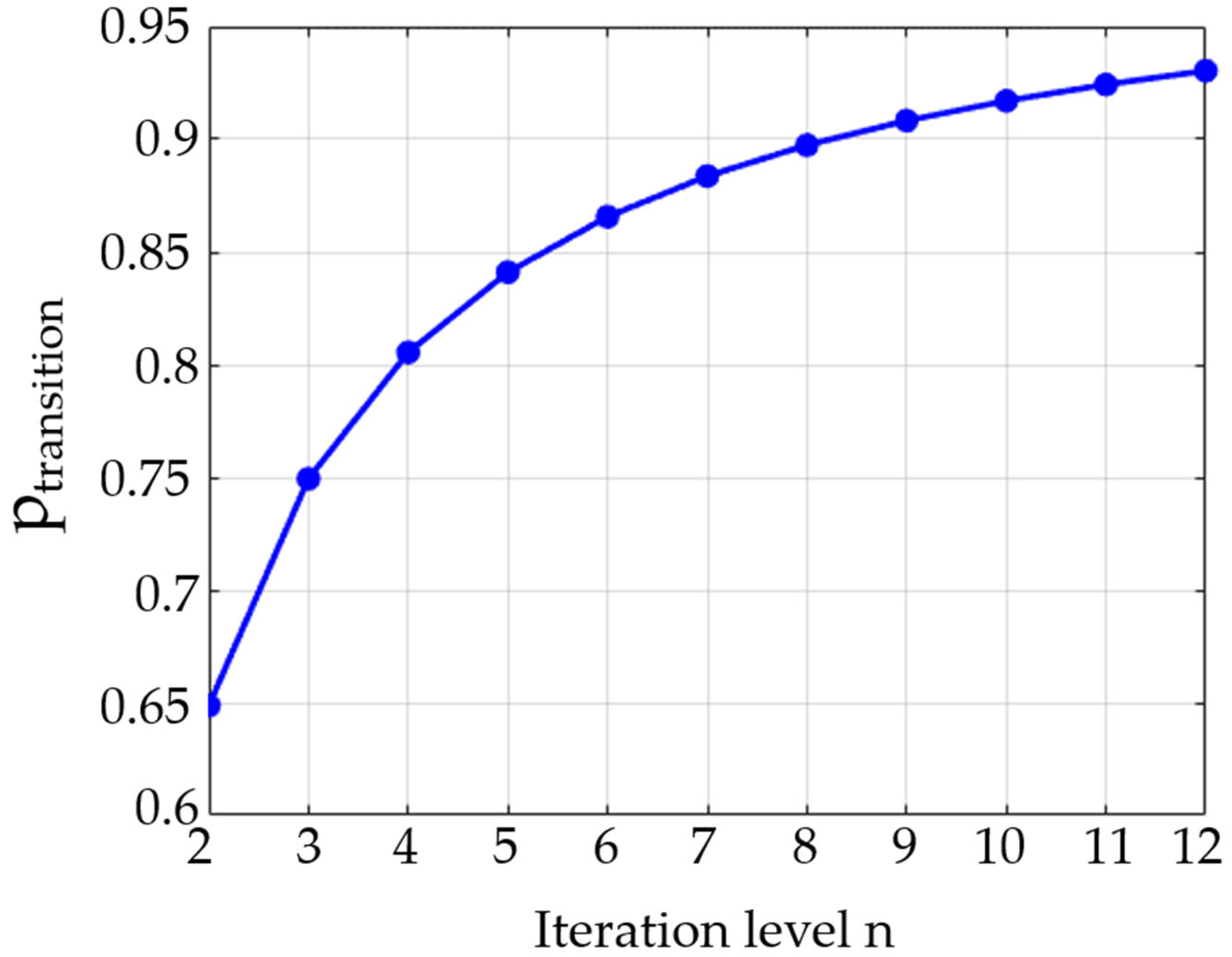
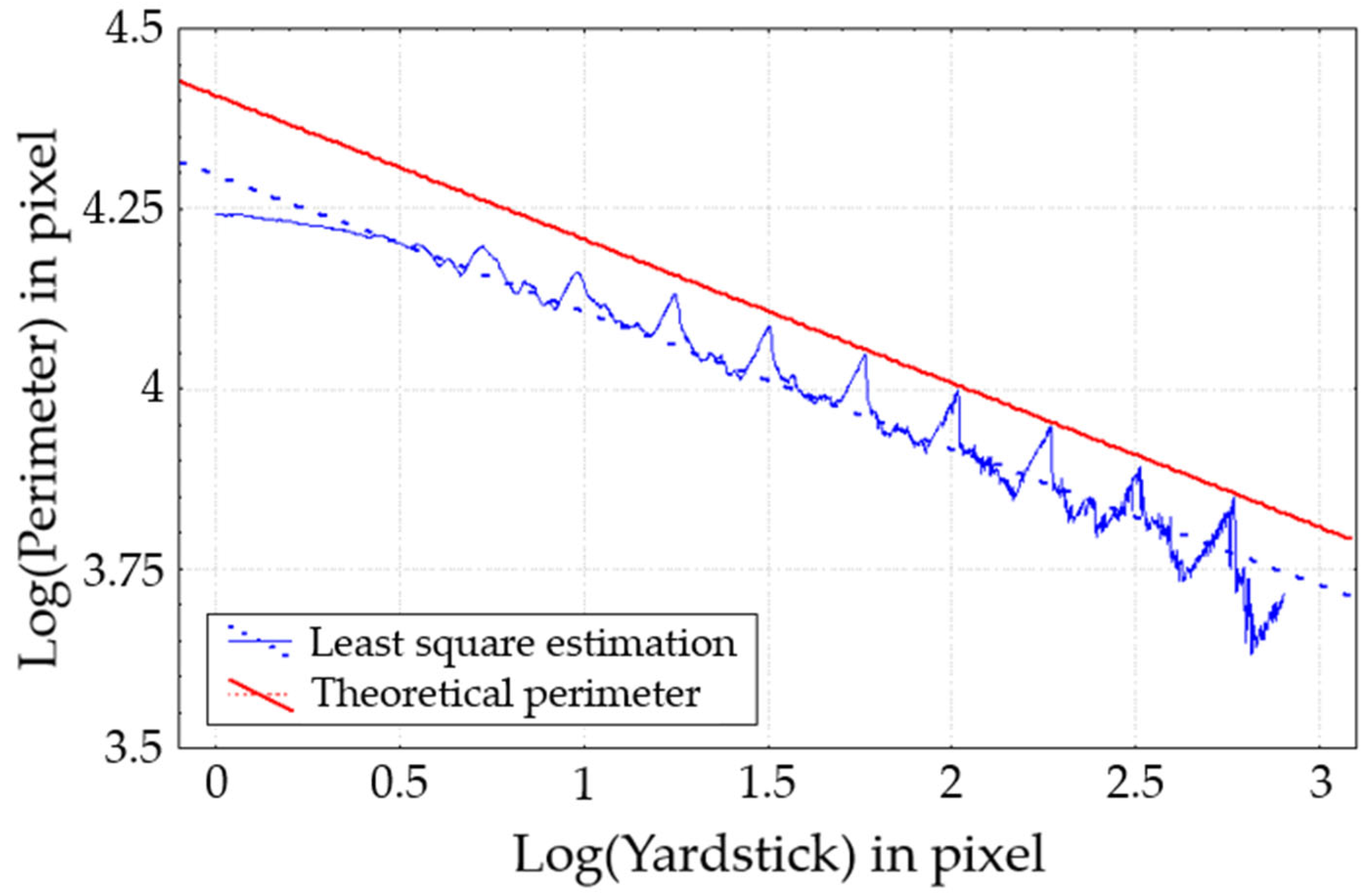
- For smaller sticks, the perimeter is increasingly underestimated as the fractal dimension grows and the underestimating range increases critically. This phenomenon is related to the length of the initiator that makes the fractal dimension grows with the smallest size of in the Koch construction. Let represent the length of the last stick after n iterations of the Koch construction. With similar principles as in Equation (1), we can lead eventually to Equation (7).
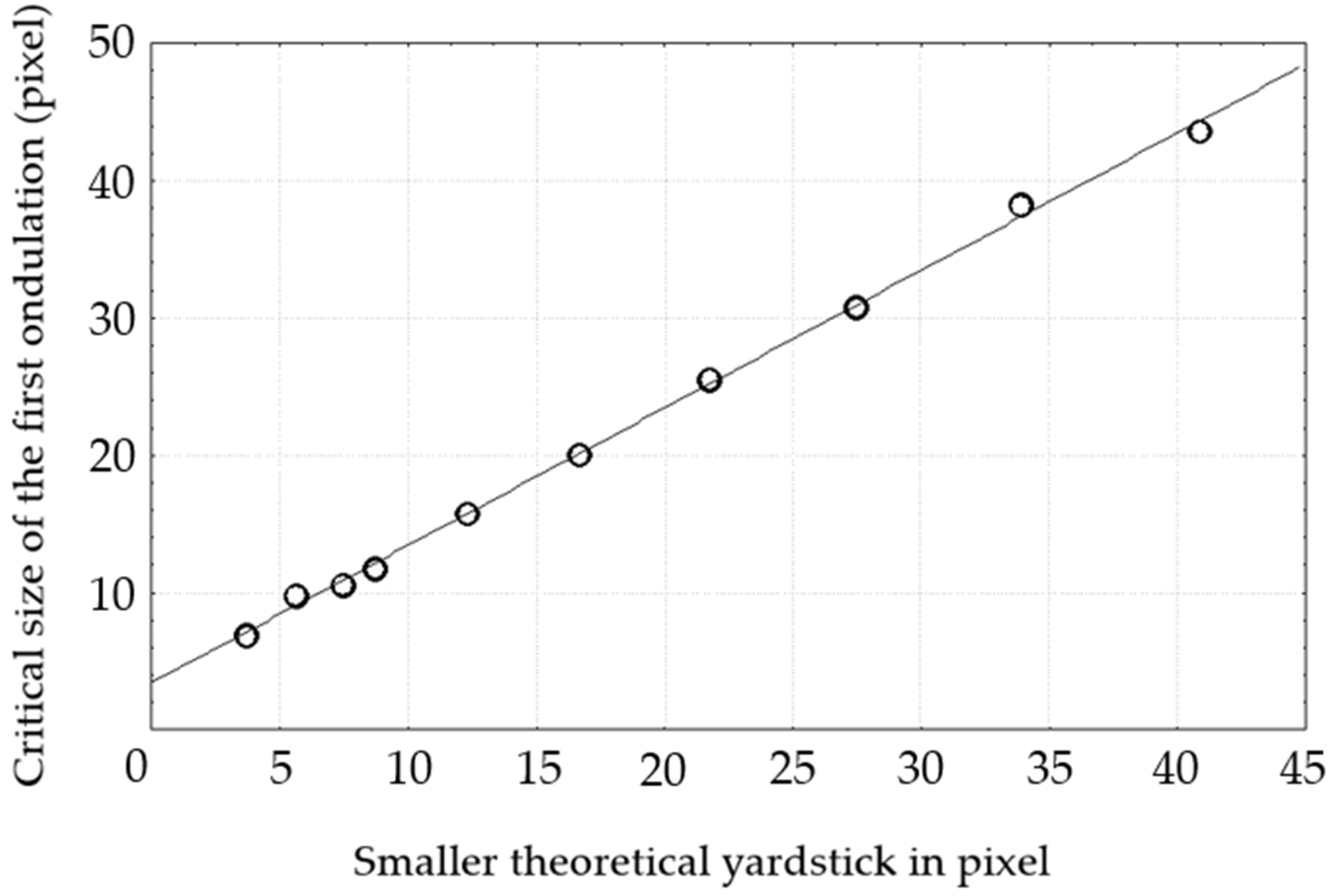
- The critical value , defined by the first significant variation in the log–log representation is plotted versus in Figure 6 (n = 5 means that five iterations are performed to construct the Von Koch Island). The very good correlation shows that the underestimation of the perimeter is a consequence of the size of the lowest initiator met in the construction of the Von Koch flake.
- 3.
- The variance in the estimation of the perimeter rises with the fractal dimension.
- 4.
- For a given yardstick, the perimeter is undervalued as the dimension increase.
3.2. Method 1: All Range of the Yardstick Variation (ARYV)
3.3. Method 2: Initiator Epsilon Min-Max Variation (IEMMV)
- The yardstick’s size must be higher than a critical value corresponding to the beginning of the fractal regime.
- The yardstick’s size must be lower than a critical size depending on the support of the fractal.
3.4. Method 3: Maximal Slope with Minimal Variation (MSMV)
3.5. Method 4: Total Maximal Slope with Minimal Variation (TMSMV)
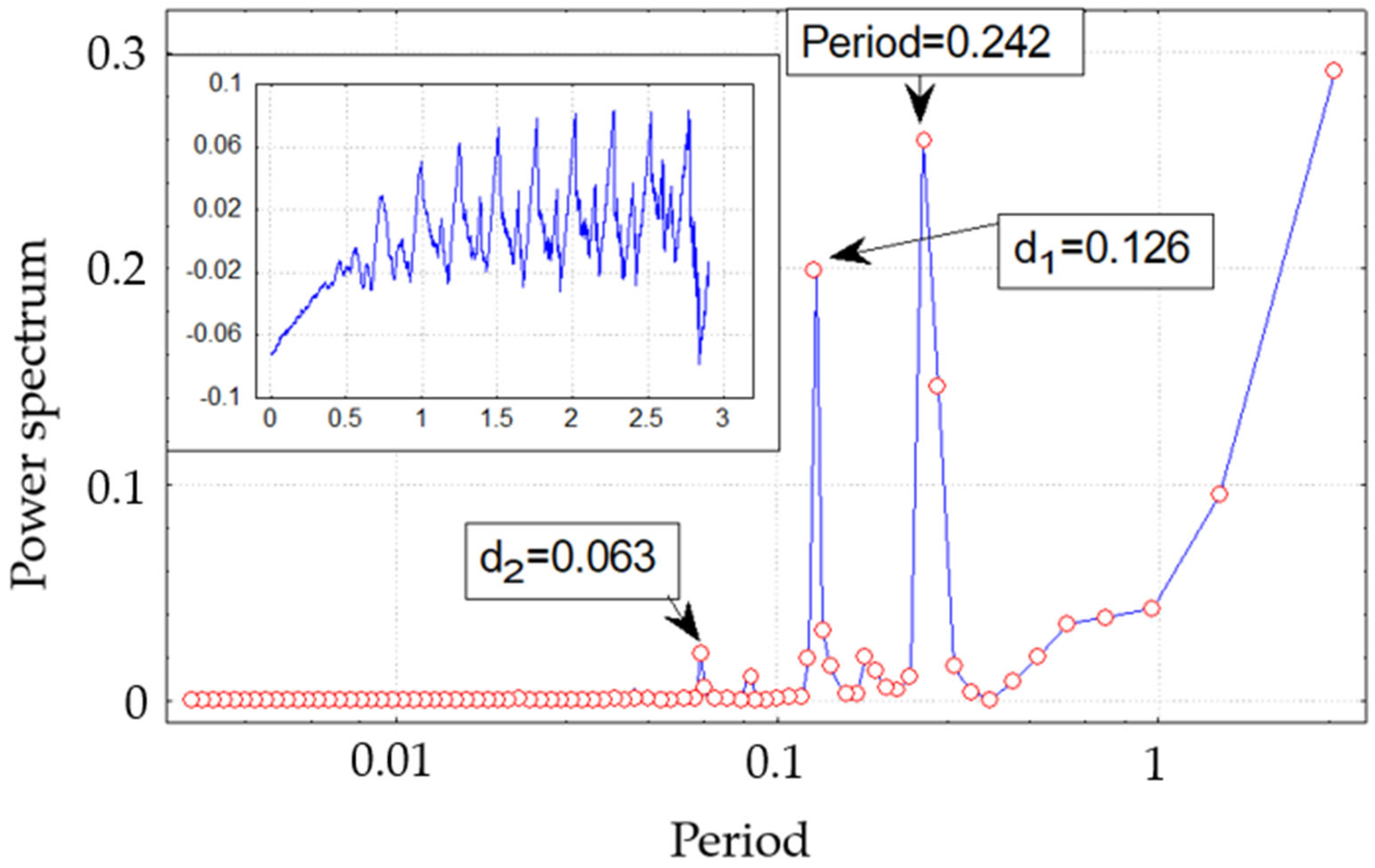
3.6. Method 5: Fourier Transform Patterns Research (FTPR)
3.7. Method 6: Self-Convolution Patterns Research (SCPR)
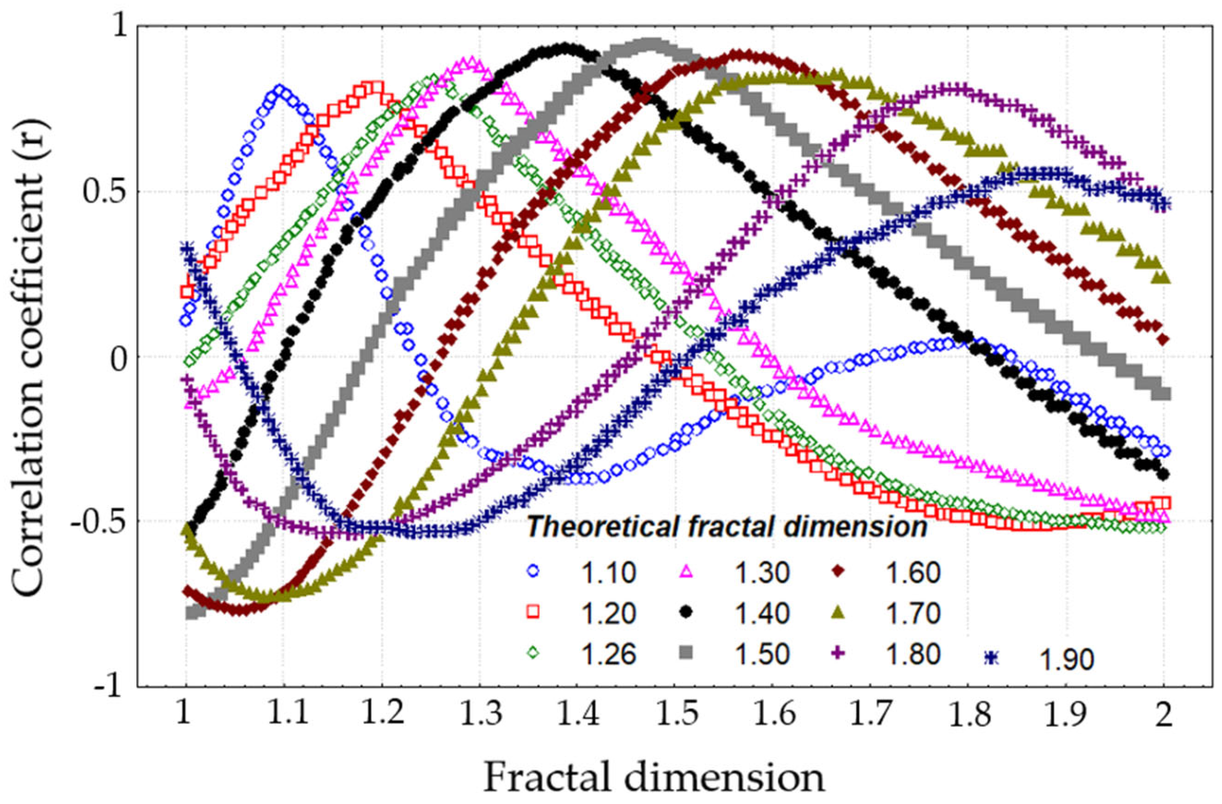
3.8. Method 7: Range Research of Optimized Fractal Dimension (RROFD)
3.9. Method 8: Total Range Research of Optimized Fractal Dimension (TRROFD)
3.10. Influence and Optimization of Yardstick Ranges
4. Analyses of the Stochastic Von Koch Flake
- 100 stochastic Von Koch flakes are constructed with five iterations and a resolution of 2048 × 2048 pixels.
- The fractal dimensions are calculated by the six different methods (ARYV, IEMMV, MSMV, TMSMV, SCPR, and TRROFD (taking the range obtained by the nearer optimization, i.e., η ∈ [37, 172]) as indicated by Method 8.
- Statistics on the 100 fractal dimensions are performed (mean, standard deviation, standard error, min, max, median, 95% confidence level for the mean) (Table 4).
5. Conclusions
Author Contributions
Funding
Data Availability Statement
Conflicts of Interest
Appendix A. Toward the Application of He–Liu Formulation in Partially Fractal Structures: The Case of the Stochastic Von Koch Curve
- When p = 1, we recover the classical dimension D = ln4/ln3,
- When p = 0, no refinement occurs, and D = 0, corresponding to a straight line (minimal complexity).

| p = 1 | p = 0.9 | p = 0.8 | p = 0.7 | p = 0.6 | p = 0.5 | p = 0.4 | p = 0.3 | p = 0.2 | p = 0.1 | p = 0 |
|---|---|---|---|---|---|---|---|---|---|---|
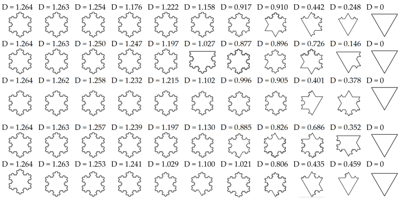 | ||||||||||

- For , the structure behaves as a partially fractal boundary, with lower geometric complexity.
- For , the effective fractal dimension saturates to that of the deterministic Koch curve, indicating full geometric development.
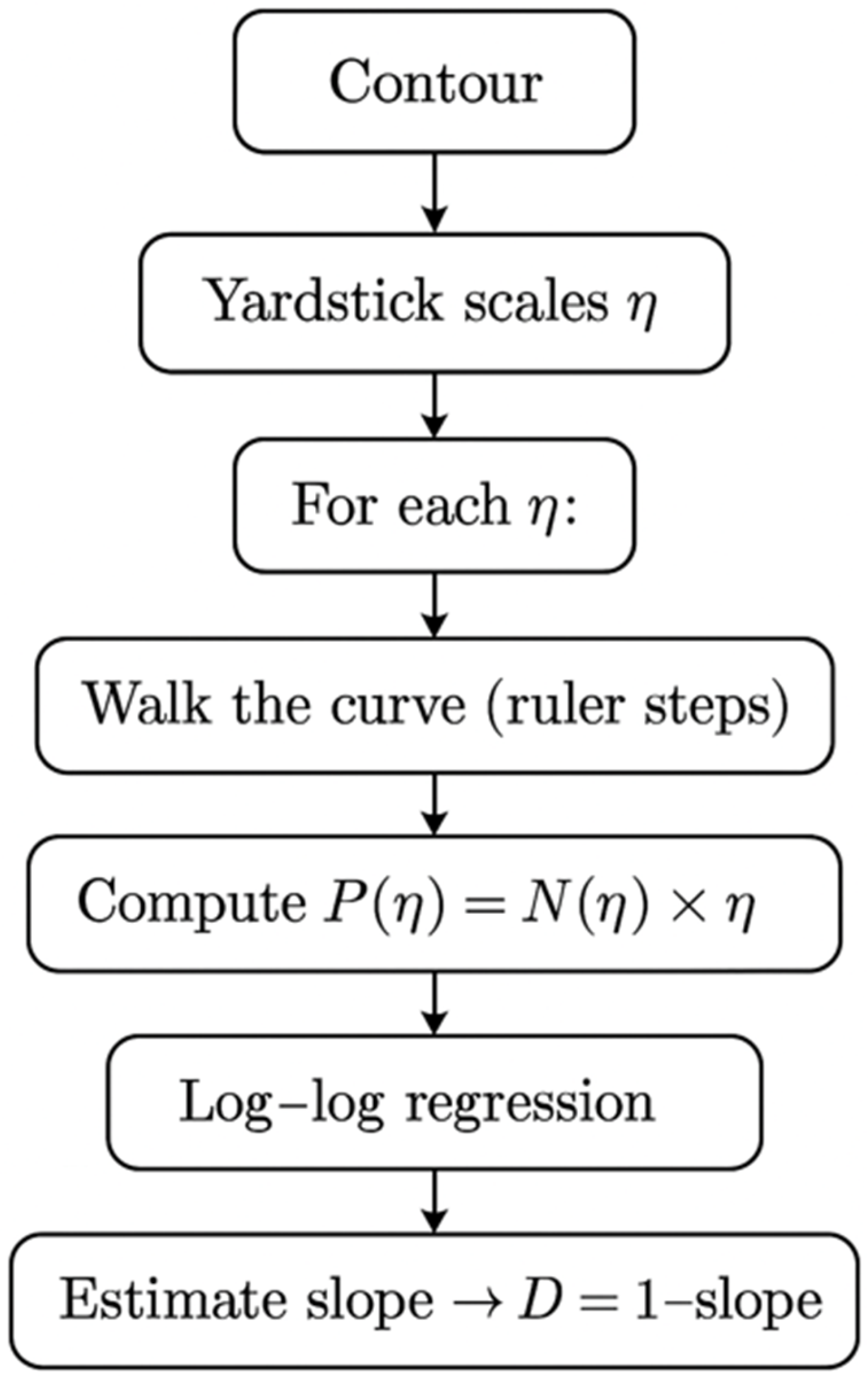
Appendix B. Algorithmic Schema of Richardson’s Method
Appendix B.1. Algorithm: Richardson–Mandelbrot (Compass) Method
- Preprocessing
- Extract the boundary or contour of the object (e.g., via edge detection or marching squares).
- Represent the contour as a sequence of ordered points
- Select yardstick sizes
- Define a set of scales , typically logarithmically spaced.
- Ensure is above image resolution noise, and below the object size.
- Traverse the contour with each yardstick
- For each , walk along the curve using a ruler of fixed length , placing steps of this size end to end.
- Count the number of steps needed to traverse the full contour.
- Compute effective perimeter
- Approximate the perimeter as .
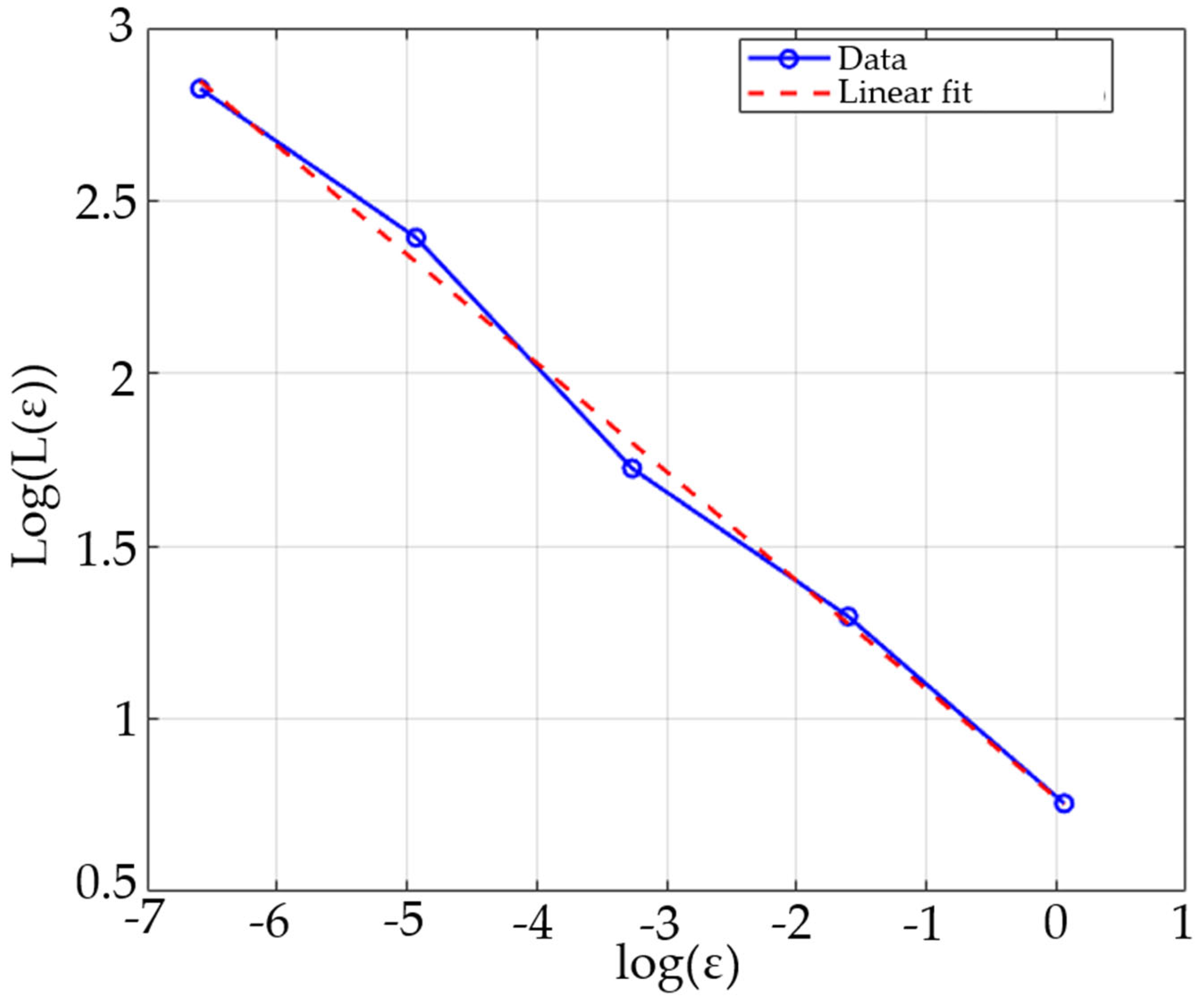
- Log–log regression
- Fit a linear regression of vs. .
- The slope s yields the fractal dimension: D = 1−s

References
- Mandelbrot, B.B. The Fractal Geometry of Nature; WH Freeman: New York, NY, USA, 1982; Volume 1. [Google Scholar]
- Li, J.; Du, Q.; Sun, C. An Improved Box-Counting Method for Image Fractal Dimension Estimation. Pattern Recognit. 2009, 42, 2460–2469. [Google Scholar] [CrossRef]
- Zhang, Z.; Wu, W.; Sun, C.; Wang, C. Seizure Detection via Deterministic Learning Feature Extraction. Pattern Recognit. 2024, 153, 110466. [Google Scholar] [CrossRef]
- Theodoridis, S.; Koutroumbas, K. Pattern Recognition; Elsevier: San Diego, CA, USA, 2006; ISBN 978-0-08-051361-4. [Google Scholar]
- Zhu, G.; Li, J.; Guo, Y. Separate First, Then Segment: An Integrity Segmentation Network for Salient Object Detection. Pattern Recognit. 2024, 150, 110328. [Google Scholar] [CrossRef]
- Tricot, C. Courbes et Dimension Fractale; Springer Science & Business Media: Berlin/Heidelberg, Germany, 1999. [Google Scholar]
- Falcão, A.X.; Stolfi, J.; de Alencar Lotufo, R. The Image Foresting Transform: Theory, Algorithms, and Applications. IEEE Trans. Pattern Anal. Mach. Intell. 2004, 26, 19–29. [Google Scholar] [CrossRef] [PubMed]
- Plotze, R.D.O.; Falvo, M.; Pádua, J.G.; Bernacci, L.C.; Vieira, M.L.C.; Oliveira, G.C.X.; Bruno, O.M. Leaf Shape Analysis Using the Multiscale Minkowski Fractal Dimension, a New Morphometric Method: A Study with Passiflora (Passifloraceae). Can. J. Bot. 2005, 83, 287–301. [Google Scholar] [CrossRef]
- Bouridane, A.; Alexander, A.; Nibouche, M.; Crookes, D. Application of Fractals to the Detection and Classification of Shoeprints. In Proceedings of the 2000 International Conference on Image Processing (Cat. No.00CH37101), Vancouver, BC, Canada, 10–13 September 2000; Volume 1, pp. 474–477. [Google Scholar]
- Shivakumara, P.; Wu, L.; Lu, T.; Tan, C.L.; Blumenstein, M.; Anami, B.S. Fractals Based Multi-Oriented Text Detection System for Recognition in Mobile Video Images. Pattern Recognit. 2017, 68, 158–174. [Google Scholar] [CrossRef]
- Backes, A.R.; Bruno, O.M. Shape Classification Using Complex Network and Multi-Scale Fractal Dimension. Pattern Recognit. Lett. 2010, 31, 44–51. [Google Scholar] [CrossRef]
- Torres, R.d.S.; Falcão, A.X.; Costa, L.d.F. A Graph-Based Approach for Multiscale Shape Analysis. Pattern Recognit. 2004, 37, 1163–1174. [Google Scholar] [CrossRef]
- Koch, H.V. Sur Une Courbe Continue sans Tangente, Obtenue Par Une Construction Géométrique Élémentaire. Ark. Mat. Astr. Fys. 1904, 1, 681–704. [Google Scholar]
- Meisel, L.V.; Johnson, M.A. Convergence of Numerical Box-Counting and Correlation Integral Multifractal Analysis Tech-niques. Pattern Recognit. 1997, 30, 1565–1570. [Google Scholar] [CrossRef]
- Mathur, V.; Gupta, M. Morphology of Koch Fractal Antenna. J. Int. J. Comput. Technol. 2014, 13, 4157–4163. [Google Scholar] [CrossRef]
- Arqub, O.A.; Abo-Hammour, Z. Numerical Solution of Systems of Second-Order Boundary Value Problems Using Continuous Genetic Algorithm. Inf. Sci. 2014, 279, 396–415. [Google Scholar] [CrossRef]
- Abo-Hammour, Z.; Arqub, O.A.; Momani, S.; Shawagfeh, N. Optimization Solution of Troesch’s and Bratu’s Problems of Ordinary Type Using Novel Continuous Genetic Algorithm. Discrete Dyn. Nat. Soc. 2014, 2014, 401696. [Google Scholar] [CrossRef]
- Carr, J.R.; Benzer, W.B. On the Practice of Estimating Fractal Dimension. Math. Geol. 1991, 23, 945–958. [Google Scholar] [CrossRef]
- Russ, J.C. Fractal Surfaces; Springer Science & Business Media: Berlin/Heidelberg, Germany, 2013; ISBN 1-4899-2578-3. [Google Scholar]
- Dubuc, B.; Dubuc, S. Error Bounds on the Estimation of Fractal Dimension. SIAM J. Numer. Anal. 1996, 33, 602–626. [Google Scholar] [CrossRef]
- Taylor, C.C.; Taylor, J. Estimating the Dimension of a Fractal. J. R. Stat. Soc. Ser. B Methodol. 1991, 53, 353–364. [Google Scholar] [CrossRef]
- Brown, C.A. Areal Fractal Methods. In Characterisation of Areal Surface Texture; Leach, R., Ed.; Springer: Berlin/Heidelberg, Germany, 2013; pp. 129–153. ISBN 978-3-642-36458-7. [Google Scholar]
- Mandelbrot, B. How Long Is the Coast of Britain? Statistical Self-Similarity and Fractional Dimension. Science 1967, 156, 636–638. [Google Scholar] [CrossRef]
- Berkmans, F.; Lemesle, J.; Guibert, R.; Wieczorowski, M.; Brown, C.; Bigerelle, M. Two 3D Fractal-Based Approaches for Topographical Characterization: Richardson Patchwork versus Sdr. Materials 2024, 17, 2386. [Google Scholar] [CrossRef]
- Bigerelle, M.; Iost, A. Perimeter Analysis of the Von Koch Island, Application to the Evolution of Grain Boundaries during Heating. J. Mater. Sci. 2006, 41, 2509–2516. [Google Scholar] [CrossRef]
- Richardson, L.F. The Problem of Contiguity: An Appendix to Statistics of Deadly Quarrels. Gen. Syst. Yearb. 1961, 6, 139–187. [Google Scholar]
- Kong, H.-Y. Research on Principle of Bubble Electrospinning and Morphologies Controlling and Applications of Bubble Electrospun Nanofibers. Ph.D. Thesis, Soochow University, Suzhou, China, 2015. [Google Scholar] [CrossRef]
- He, C.-H.; Liu, H.-W.; Liu, C. A Fractal-Based Approach to the Mechanical Properties of Recycled Aggregate Concretes. Facta Univ. Ser. Mech. Eng. 2024, 22, 329–342. [Google Scholar] [CrossRef]


| 1 ARYV | 2 IEMMV | 3 MSMV | 4 TMSMV | 5 FTPR | 6 SCPR | 7 RROFD | 8 TRROFD | ||||||
|---|---|---|---|---|---|---|---|---|---|---|---|---|---|
| Δt | Δc | ηmin ηmax | Δc | ηmin ηmax | Δc | ηmin ηmax | Δc | ηmin ηmax | Δc | Δc | ηmin ηmax | Δc | ηmin ηmax |
| 1.1 | 1.102 | 1 800 | 1.101 | 4 580 | 1.099 | 1 580 | 1.102 | 1 800 | 1.141 | 1.096 | 27 187 | 1.098 | 37 172 |
| 1.2 | 1.181 | 1 800 | 1.188 | 6 573 | 1.183 | 2 573 | 1.189 | 2 800 | 1.244 | 1.197 | 69 712 | 1.187 | 37 172 |
| 1.26 | 1.224 | 1 800 | 1.241 | 8 609 | 1.231 | 2 609 | 1.243 | 3 800 | 1.244 | 1.255 | 53 724 | 1.260 | 37 172 |
| 1.3 | 1.248 | 1 800 | 1.275 | 9 619 | 1.267 | 4 619 | 1.285 | 9 800 | 1.244 | 1.295 | 38 259 | 1.318 | 37 172 |
| 1.4 | 1.306 | 1 800 | 1.368 | 13 645 | 1.352 | 5 645 | 1.359 | 5 800 | 1.348 | 1.396 | 44 362 | 1.367 | 37 172 |
| 1.5 | 1.352 | 1 800 | 1.459 | 17 672 | 1.438 | 7 672 | 1.457 | 10 800 | 1.452 | 1.480 | 59 343 | 1.444 | 37 172 |
| 1.6 | 1.389 | 1 800 | 1.555 | 22 681 | 1.537 | 14 691 | 1.543 | 13 800 | 1.555 | 1.581 | 64 380 | 1.583 | 37 172 |
| 1.7 | 1.417 | 1 800 | 1.647 | 28 717 | 1.644 | 24 717 | 1.652 | 24 800 | 1.659 | 1.671 | 75 408 | 1.692 | 37 172 |
| 1.8 | 1.439 | 1 800 | 1.738 | 34 737 | 1.737 | 30 737 | 1.743 | 30 800 | 1.763 | 1.786 | 40 179 | 1.792 | 37 172 |
| 1.9 | 1.462 | 1 800 | 1.816 | 41 755 | 1.826 | 35 755 | 1.825 | 35 800 | 1.866 | 1.901 | 36 187 | 1.893 | 37 172 |
| ∆ | dtheo | dmean | dinf | dsup | ∆c | ∆inf | ∆sup |
|---|---|---|---|---|---|---|---|
| 1.10 | 0.274 | 0.264 | 0.242 | 0.290 | 1.14 | 1.04 | 1.24 |
| 1.20 | 0.251 | 0.242 | 0.223 | 0.264 | 1.24 | 1.14 | 1.35 |
| 1.26 | 0.239 | 0.242 | 0.223 | 0.264 | 1.24 | 1.14 | 1.35 |
| 1.30 | 0.232 | 0.242 | 0.223 | 0.264 | 1.24 | 1.14 | 1.35 |
| 1.40 | 0.215 | 0.223 | 0.207 | 0.242 | 1.35 | 1.24 | 1.45 |
| 1.50 | 0.201 | 0.207 | 0.193 | 0.223 | 1.45 | 1.35 | 1.56 |
| 1.60 | 0.188 | 0.194 | 0.181 | 0.207 | 1.56 | 1.45 | 1.66 |
| 1.70 | 0.177 | 0.181 | 0.171 | 0.194 | 1.66 | 1.56 | 1.76 |
| 1.80 | 0.167 | 0.171 | 0.161 | 0.181 | 1.76 | 1.66 | 1.87 |
| 1.90 | 0.158 | 0.161 | 0.153 | 0.171 | 1.87 | 1.76 | 1.97 |
| Method | Full Name | Description | ||
|---|---|---|---|---|
| 1. ARYV | All Range of the Yardstick Variation | Fixed (e.g., 1 pixel) | Fixed (e.g., 800 pixels) | Full range arbitrarily chosen; prone to errors due to discretization (low η) or oversmoothing (high η). |
| 2. IEMMV | Initiator Epsilon Min-Max Variation | ε5 = smallest segment of the generator (iteration 5) | ε1 = initial segment of the initiator | Requires knowledge of the fractal’s construction parameters; not usable on unknown curves. |
| 3. MSMV | Maximal Slope with Minimal Variation | Selected to minimize slope variance | Selected to minimize slope variance | Searches for stable intervals with low slope fluctuation, without relying on explicit geometric knowledge. |
| 4. TMSMV | Total Maximal Slope with Minimal Variation | Like MSMV | Fixed at 800 pixels | More general version of MSMV that can be applied to unknown or experimental fractals. |
| 5. FTPR | Fourier Transform Pattern Research | Implicit (derived from residuals) | Implicit (derived from residuals) | No explicit η range; analysis is based on the periodicity of residuals in the log–log perimeter plot. |
| 6. SCPR | Self-Convolution Patterns Research | Determined automatically via autocorrelation | Determined automatically via autocorrelation | Peak lag are implicit from the correlated signal. |
| 7. RROFD | Range Research of Optimized Fractal Dimension | Explored by grid search | Explored by grid search | Optimized per curve to find the best interval with minimal deviation from theoretical D. |
| 8. TRROFD | Total Range Research of Optimized Fractal Dimension | = 37 pixels | = 172 pixels | Globally optimized range that minimizes average error across all tested fractal dimensions; provides stable and general recommendation. |
| Method | Mean | −IC 95% | + IC 95% | Median | Minimum | Maximum | Std Dev |
|---|---|---|---|---|---|---|---|
| ARYV | 1.186945 | 1.186567 | 1.187322 | 1.186793 | 1.182414 | 1.192838 | 0.001892 |
| TMSMV | 1.197857 | 1.197272 | 1.198442 | 1.197949 | 1.191600 | 1.207049 | 0.002932 |
| SCPR | 1.199980 | 1.198943 | 1.201017 | 1.198000 | 1.191000 | 1.212000 | 0.005200 |
| TRROFD | 1.197210 | 1.195674 | 1.198745 | 1.196271 | 1.180984 | 1.214840 | 0.007698 |
| IEMMV | 1.196716 | 1.196080 | 1.197351 | 1.196651 | 1.190029 | 1.207746 | 0.003184 |
| MSMV | 1.180796 | 1.180464 | 1.181128 | 1.180775 | 1.177221 | 1.185031 | 0.001665 |
Disclaimer/Publisher’s Note: The statements, opinions and data contained in all publications are solely those of the individual author(s) and contributor(s) and not of MDPI and/or the editor(s). MDPI and/or the editor(s) disclaim responsibility for any injury to people or property resulting from any ideas, methods, instructions or products referred to in the content. |
© 2025 by the authors. Licensee MDPI, Basel, Switzerland. This article is an open access article distributed under the terms and conditions of the Creative Commons Attribution (CC BY) license (https://creativecommons.org/licenses/by/4.0/).
Share and Cite
Bigerelle, M.; Berkmans, F.; Lemesle, J. Evaluating the Fractal Pattern of the Von Koch Island Using Richardson’s Method. Fractal Fract. 2025, 9, 483. https://doi.org/10.3390/fractalfract9080483
Bigerelle M, Berkmans F, Lemesle J. Evaluating the Fractal Pattern of the Von Koch Island Using Richardson’s Method. Fractal and Fractional. 2025; 9(8):483. https://doi.org/10.3390/fractalfract9080483
Chicago/Turabian StyleBigerelle, Maxence, François Berkmans, and Julie Lemesle. 2025. "Evaluating the Fractal Pattern of the Von Koch Island Using Richardson’s Method" Fractal and Fractional 9, no. 8: 483. https://doi.org/10.3390/fractalfract9080483
APA StyleBigerelle, M., Berkmans, F., & Lemesle, J. (2025). Evaluating the Fractal Pattern of the Von Koch Island Using Richardson’s Method. Fractal and Fractional, 9(8), 483. https://doi.org/10.3390/fractalfract9080483