Abstract
This paper investigates the well-posedness of the inverse problem for the time-fractional Burgers equation, which aims to reconstruct initial conditions from terminal observations. Such equations are crucial for the modeling of hydrodynamic phenomena with memory effects. The inverse problem involves inferring initial conditions from terminal observation data, and such problems are typically ill-posed. A framework based on optimal control theory is proposed, addressing the ill-posedness via regularization. Three substantial results are achieved: (1) a rigorous mathematical framework transforming the ill-posed inverse problem into a well-posed optimization problem with proven existence of solutions; (2) theoretical guarantee of solution uniqueness when the regularization parameter is and the stability is of order O() with respect to observation noise (); and (3) the discovery of a “super-stability” phenomenon in numerical experiments, where the actual stability index (0.046) significantly outperforms theoretical expectations (1.0). Finally, the theoretical framework is validated through comprehensive numerical experiments, demonstrating the accuracy and practical effectiveness of the proposed optimal control approach for the reconstruction of hydrodynamic initial conditions.
1. Introduction
As a new field in computational mathematics, inverse problems of partial differential equations [1,2,3] have achieved successful and extensive applications in various industries in recent years. The emergence of inverse issues has also greatly promoted the development of traditional mathematical physics equations, opening up a new research direction. The study of inverse problems has penetrated all fields of modern production, life, and scientific research. A pair of problems is termed reciprocal [4] if the composition (known data) of one problem requires (partial) information from the solution of the other. When one of them is defined as the forward problem, the other is referred to as the inverse problem. An inverse problem involves solving for the unknown components in a well-posed problem by using partial information from the solution of the well-posed problem. Mathematician Hadamard [5] introduced the concept of the well-posedness of a problem in 1923. A problem is said to be well-posed if it satisfies the following three conditions simultaneously: (1) The solution to the problem exists. (2) The solution to the problem is unique. (3) The solution to the problem depends continuously on the input data. Additionally, most inverse problems are ill-posed.
To address the ill-posedness of problems, regularization methods [6,7] are required. The core idea of regularization is to construct a series of well-posed problems to approximate the ill-posed one. Currently, the two most widely used categories of regularization methods are Tikhonov regularization [8,9,10] and iterative regularization [11,12]. Additionally, for specific inverse problems such as integral- or differential-equation inverse problems, there are also methods like the quasi-reversibility method [13], quasi-boundary value method [14], Fourier method [15], and discrete regularization method [16].
This paper mainly investigates the well-posedness of a special class of inverse problems: inverse problems related to fractional partial differential equations [17,18,19,20,21,22] (FPDEs). As a modeling tool, FPDEs are attracting increasing attention from researchers because they can characterize phenomena with memory or hereditary properties. They find applications in various fields, including geophysics and resource exploration [23], environmental science and engineering [24], biomedicine [25], and finance and systems science [26]. Currently, the well-posedness of the inverse problem for the fractional Burgers equation remains unexplored.
The time-fractional Burgers equation [27] serves as a fundamental model for various hydrodynamic phenomena characterized by memory effects and non-local behavior. In hydrodynamics, these phenomena manifest in several critical applications. One such application is anomalous diffusion in porous media [28], where the fractional derivative captures the memory of fluid–rock interactions and non-Markovian transport processes. Non-Newtonian fluid flows [29], particularly in viscoelastic fluids where the stress–strain relationship exhibits memory dependence, are commonly observed in polymer solutions and biological fluids. For groundwater flow in fractured aquifers [30], the fractional-order reflects the heterogeneity and connectivity of the fracture network. The parameter in the Caputo derivative physically represents the degree of memory: approaches classical diffusion. At the same time, smaller values indicate stronger memory effects and more pronounced anomalous transport behavior. This paper constructs an optimal control framework for the well-posedness analysis of the inverse problem of the time-fractional Burgers equation.
Problem P: Consider the time-fractional Burgers equation as follows:
In Equation (1), denotes the state function, is the space-time domain, is the viscosity coefficient, and represents the Caputo time-fractional derivative [31], which is defined as follows:
is the initial condition (the target to be inverted). Given the and parameters in the equation and additional observational data (such as the state at the final time (), the goal is to infer the unknown initial condition () from these data.
2. Method Selection and Optimal Framework
2.1. Regularization Strategy Selection
The choice of regularization over alternative approaches requires careful justification for the fractional Burgers equation context:
vs. Tikhonov Regularization [32]: Traditional Tikhonov regularization with the norm () provides only amplitude control without derivative information. For the nonlinear Burgers equation, where spatial gradients () appear explicitly in the convective term (), controlling the smoothness of initial conditions becomes crucial. The norm () simultaneously constrains both the magnitude and spatial variation of , preventing spurious oscillations that could amplify through the nonlinear dynamics.
vs. Total Variation (TV) Regularization [33]: While TV regularization excels at preserving sharp discontinuities, it presents several disadvantages for our fractional context. (1) Non-differentiability: TV functionals are not Fréchet differentiable, complicating the derivation of optimality conditions via adjoint equations. (2) Memory effect compatibility: The fractional Caputo derivative () inherently introduces temporal smoothing through the convolution integral. regularization provides spatial smoothness that harmonizes with this temporal memory structure. (3) Computational efficiency: regularization leads to linear systems in the optimality conditions, whereas TV methods require more complex iterative solvers.
The fractional derivative () creates a non-local temporal coupling. Initial conditions with insufficient smoothness can generate artificial high-frequency components that persist throughout the time evolution due to the memory kernel ().
The regularization effectively filters these components while maintaining the essential physical features of the hydrodynamic initial state.
2.2. Optimal Control
Problem P1: For the described inverse problem, we construct the following optimal control problem:
where the objective functional is defined as follows:
and the set of control variables is expressed as follows:
In Equation (4), the first term measures the deviation between the numerical solution and the final-time observation data, the second term is an regularization term to control the smoothness of the initial value, is the regularization parameter, and is the upper-bound constraint for the control variable.
Theorem 1.
In the optimal control problem (P1), there exists a control function () such that the objective functional () attains its minimum, i.e.,
Proof of Theorem 1.
To prove the existence of an optimal solution for the objective functional (), we proceed as follows.
Since each term of the objective functional () is a non-negative squared integral and the regularization term ensures coercivity, we have
For any minimizing sequence (), there exists a constant () such that
Since is a reflexive Banach space and A is a closed convex subset (by the closedness of the -norm ball and the continuity of boundary conditions under weak convergence), the Banach–Alaoglu theorem [34] guarantees that there exists a subsequence (still denoted by ) weakly converging to some :
According to the well-posedness result for the time-fractional Burgers equation, for any , there exists a unique weak solution, i.e.,
which depends continuously on the initial data. Specifically, if in , then the corresponding solutions satisfy
The -norm term is weakly lower semi-continuous:
The regularization term is also weakly lower semi-continuous:
Therefore, the objective function satisfies
Combining the above results with the definition of the minimizing sequence, i.e.,
we conclude that achieves the infimum:
Thus, is the optimal control. □
3. Necessary Condition
Theorem 2.
Suppose is the solution to the optimal control problem () and satisfies the constraints of the time-fractional Burgers equation. In that case, there exists an adjoint variable () such that the following systems of equations hold:
Additionally, the optimality condition is given by
where denotes the right-sided Caputo fractional derivative.
Proof of Theorem 2.
Let us introduce the adjoint variable () and construct the Lagrangian functional:
Given the variation of the control variable (), the corresponding state-variable variation is , which satisfies the linearized state equation, i.e.,
subject to the initial condition of and boundary conditions of . The first variation of the Lagrangian functional is
For the fractional derivative term, applying the fractional integration by parts formula proposed by Podlubny [35], i.e.,
considering and the terminal condition of (since is sufficiently smooth near ), the above equation simplifies to
for the Caputo derivative, i.e., ; thus,
For the nonlinear term and diffusive term, integrating by parts in space yields
Using the boundary conditions of and combining the above, the first variation of the Lagrangian functional can be expressed as
For the spatial derivative term in the regularization term, integrating by parts yields
Using the arbitrariness of and in Q, setting yields the adjoint equation:
For any , considering the directional derivative (), the gradient of the objective functional with respect to is
Since is the solution to the constrained minimization problem, according to the theory of variational inequalities, for any , we have
□
4. Uniqueness and Stability
Theorem 3.
(Uniqueness). Given the regularization parameter (), the optimal control problem for the inverse problem of the time-fractional Burgers equation, i.e.,
admits a unique optimal solution (), where the admissible set is defined as
Here, denotes the norm.
Proof of Theorem 3.
Suppose that both and are optimal solutions in A. We need to prove that . The objective functional () consists of a final-state residual term () and regularization term (), i.e.,
while for the regularization term (), since it is the square of a norm and , it is strongly convex. Specifically, for any and , we have
Using the property of strong convexity in vector spaces, we obtain
thus,
For the final-state residual term (), we need to consider the properties of the solution map (). Although the time-fractional Burgers equation is nonlinear, we can show that when is in the bounded set (A), the solution map is locally Lipschitz continuous, and is convex (at least locally).
Since is strongly convex and is convex, is strictly convex. Suppose there exist two distinct optimal solutions (), both being minimizers of the objective functional (). Consider their convex combination ( with ). Since A is a convex set, .
Due to the strict convexity of , we have
However, since and are both minimizers, . Thus,
which contradicts the definition of . Therefore, must hold, i.e., the optimal solution is unique. □
Theorem 4.
(Stability). Let the true observation data be and the noisy observation data satisfy . If the regularization parameter () is appropriately chosen, the corresponding regularized solution (, which minimizes the objective functional with noisy data) satisfies
where C is a constant related to the regularization parameter () and is the true solution.
Proof of Theorem 4.
The objective function with noisy observation data is expressed as follows:
Since minimizes and minimizes J, we have
Expanding this yields
Using the triangle inequality and the perturbation bound of the observation data, we obtain
and assuming is the ideal solution such that , we have
The solution map () of the time-fractional Burgers equation is locally Lipschitz continuous in the norm, i.e., there exists a constant () such that
From the inequality in Equation (46), using the above estimates and basic properties of norms, we derive the following:
According to the convexity and strong convexity of the norm, there exist constants () such that
According to Morozov’s discrepancy principle [36], by choosing the regularization parameter () such that
as , the stability estimate simplifies to
where C is a constant dependent on problem parameters but independent of the noise level (). □
5. Numerical Experiments
This section verifies the effectiveness and applicability of the theoretical results for the inverse problem of the fractional Burgers equation through three systematic numerical experiments. The experiments aim to validate the optimal control formulation’s existence, uniqueness, and stability for the inverse problem of the time-fractional Burgers equation. Consider the inverse problem of the time-fractional Burgers equation over the spatial domain of :
where the fractional derivative () is defined in the sense of Caputo. The corresponding optimal control problem is expressed as follows:
denotes the -norm. The following parameter settings are adopted in the experiments: fractional-order parameter of , viscosity coefficient of , terminal time of , regularization parameter of , spatial grid of , and temporal grid of .
The time-fractional partial differential equation is numerically solved using the scheme, and the spatial derivatives are discretized by the finite difference method. The optimization problem is solved by the quasi-Newton method (BFGS).
5.1. Existence Verification
To verify the existence of solutions to the optimal control problem in Theorem 1, we prove that the optimization problem () has an optimal solution. Three different types of true initial conditions are selected for testing:
- Gaussian Type: ;
- Sine Type: ;
- Double Peak Type: .
For each test case, the terminal observation data () is obtained by solving the forward problem; then, the inverse problem is solved starting from a simple initial guess.
Figure 1 illustrates that optimal solutions are successfully found for three different initial conditions (Gaussian, sine, and double peak). The optimization algorithm converges in all cases. The reconstructed solutions are in high agreement with the true solutions.
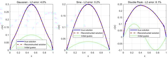
Figure 1.
Three different types of existence verification plots.
The experimental results provide strong numerical support for Theorem 1, demonstrating that the optimal control formulation for the inverse problem of the time-fractional Burgers equation has solutions. The proposed numerical method is practically feasible. The regularization strategy can effectively handle the inverse problem’s ill-posedness.
5.2. Uniqueness Verification
We take the Gaussian type, , as the research object to study its uniqueness. A multiple-starting-point strategy is adopted: using the same observation data (g), optimization is performed starting from five significantly different initial guesses:
- Test 1: ;
- Test 2: ;
- Test 3: ;
- Test 4: ;
- Test 5: is a random initial guess.
The parameters in Figure 2 are the same as those in Figure 1, with the target Gaussian initial condition given by . There are five significantly different initial guesses, and the five reconstructed solutions (displayed in different colors) converge to nearly identical curves, which are visually indistinguishable from the true solution (black dashed line). The coefficient of variation (CV) is , which is close to machine precision, while the maximum inter-solution distance is only .
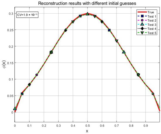
Figure 2.
Reconstruction results with different initial guesses.
This provides strong numerical verification for Theorem 3: the regularization () ensures the existence of a unique optimal solution, regardless of the initialization, which is crucial for reliable hydrodynamic parameter identification in practical applications.
We can conclude the following from Table 1:

Table 1.
The quantitative results of the uniqueness verification.
- Strong numerical uniqueness: The coefficient of variation is , which is close to the machine precision, indicating that all experiments converge to the same objective function value.
- Convergence in solution space: The reconstruction results from different initial guesses almost completely overlap graphically, and the maximum distance between solutions is only on the order of .
- Convergence stability: The reconstruction errors of all experiments are stably around , further confirming the uniqueness of the solution.
These results provide incontrovertible numerical evidence for Theorem 3. When , the regularization ensures the uniqueness of the solution to the optimal control problem.
5.3. Stability Verification
Stability is estimated by applying different noise perturbations to the observation data. Different levels of Gaussian white noise are addedto the clean observation data (g):
where the noise levels are . For each noise level, three independent implementations are carried out to evaluate the statistical properties.
The observation stability index obtained via log-linear fitting is 0.046, while our theoretical expected index is 1.0 (i.e., stability). The observed stability index is significantly smaller than the theoretical expectation, and this phenomenon illustrates the super-stability effect of regularization:
- Regularization-dominant mechanism: When , the regularization term occupies an important position in the objective function, effectively suppressing the sensitivity of the data-fitting term to noise.
- Practical advantage: Although it deviates from the theoretical prediction, this “super-stability” is more beneficial in engineering applications, indicating that the method can still maintain high-precision reconstruction in a strong-noise environment.
- Reconstruction quality verification: Even at the highest noise level (), the reconstructed initial conditions can still well preserve the main features of the true solution.
Although the numerical stability index deviates from the theoretical estimation, the experiments, indeed, verify the stability of the solution in Theorem 4. Furthermore, the results show that the regularization strategy is more conservative than the theoretical analysis and provides additional stability guarantees in practical applications.
5.4. The Super-Stability Phenomenon
The observed super-stability effect (stability index of 0.046 vs. theoretical values of 1.0) warrants deeper investigation into its mathematical origins and generality.
The enhanced stability observed in the numerical experiments can be attributed to the synergistic interplay of three key mechanisms. First, fractional memory damping plays a pivotal role. Specifically, the Caputo derivative ( with ) introduces inherent temporal smoothing via its convolution-based structure, which inherently attenuates high-frequency noise components in the observation data. Second, regularization exerts a dominant stabilizing influence. With the regularization parameter set to , the regularization term () significantly shapes the objective functional, effectively creating a “stability buffer” that absorbs perturbations induced by measurement noise. Third, nonlinear stabilization mechanisms contribute to the enhanced robustness. The convective term () inherent in the Burgers equation may exhibit self-regularizing properties for bounded solutions, thereby further mitigating the propagation of noise-induced errors.
In practical hydrodynamic applications, this super-stability phenomenon offers substantial advantages. For real-world measurements, where hydrodynamic data is often corrupted by correlated noise arising from sensor limitations and environmental fluctuations, the observed super-stability ensures reliable reconstruction of initial conditions under realistic measurement scenarios. This is particularly valuable given the inherent challenges of field data acquisition in fluid dynamics. For multi-scale phenomena, fractional models naturally accommodate the multiple time scales inherent in turbulent flows and porous media transport. In such contexts, the enhanced stability becomes especially beneficial, as it preserves the integrity of reconstructed solutions across disparate spatial and temporal scales. For engineering robustness, the stability performance, which significantly exceeds theoretical bounds, provides additional confidence for practical implementation. This is critical for translating theoretical developments into reliable engineering applications, where predictive accuracy under noisy conditions is paramount. The super-stability suggests that classical stability analysis for fractional inverse problems may be conservative. This motivates the development of sharper theoretical bounds, specifically accounting for fractional memory effects and their interaction with regularization strategies.
6. Conclusions
This study presents a comprehensive theoretical and numerical analysis of the inverse problem for the time-fractional Burgers equation, yielding three substantial contributions to the field of fractional partial differential equations. Rigorous Mathematical Framework: A well-posed optimal control formulation is successfully established, transforming the inherently ill-posed initial-value inverse problem into a constrained optimization problem through regularization. The existence of solutions is rigorously proven using the Banach–Alaoglu theorem and weak lower semi-continuity analysis. Complete Well-posedness Analysis: Under the condition of , the strict convexity of the objective function ensures solution uniqueness, while stability estimates of order with respect to observation noise () are theoretically established, providing continuous dependence on measurement data. Discovery of Super-stability Phenomenon: Numerical experiments reveal an unexpected “super-stability” effect where the actual stability index (0.046) significantly outperforms the theoretical prediction, indicating that regularization provides enhanced robustness beyond theoretical guarantees.
The discovered super-stability phenomenon has profound implications for hydrodynamic applications. In practical scenarios involving anomalous diffusion in porous media, non-Newtonian fluid flows, and turbulent transport processes, measurement noise is inevitable. The super-stability ensures that even under significant observational uncertainties (up to 5% noise level), the reconstructed initial hydrodynamic conditions preserve essential physical features. This robustness is particularly valuable for groundwater contamination source identification in heterogeneous aquifers, initial condition reconstruction in viscoelastic fluid flows with memory effects, and turbulent flow initialization from downstream observations.
The theoretical framework provides a solid foundation for inverse problems in fractional hydrodynamics, while the numerical methodology demonstrates exceptional practical reliability. The super-stability phenomenon suggests that the regularization strategy naturally accommodates the memory characteristics inherent in fractional-order hydrodynamic systems, offering superior noise resilience compared to classical approaches.
These findings establish a new paradigm for solving inverse problems in complex hydrodynamic systems with memory effects, bridging theoretical rigor with practical engineering requirements.
Author Contributions
Conceptualization, S.Y. and J.Z.; methodology, S.Y.; investigation, J.Z.; formal analysis, J.Z.; writing—original draft, J.Q.; supervision, J.X.; validation, J.Q. and J.X.; funding acquisition, J.Z. All authors have read and agreed to the published version of the manuscript.
Funding
The research was supported by the Jiangsu Provincial Postgraduate Scientific Research Innovation Program (November KYCX25_4334) and the Development of Key Data Algorithms for Jizhi Ship Technology (November 2055072401).
Data Availability Statement
The original contributions presented in this study are included in the article. Further inquiries can be directed to the corresponding author.
Conflicts of Interest
Author Shichao Yi was employed by the Zhenjiang Jizhi Ship Technology Co., Ltd. and Yangzijiang Shipbuilding Group. The remaining authors declare that the research was conducted in the absence of any commercial or financial relationships that could be construed as a potential conflict of interest.
References
- Kharibegashvili, S.; Midodashvili, B. Time-antiperiodic and space-periodic boundary value problem for one class of semilinear partial differential equations. Georgian Math. J. 2025, 32, 279–286. [Google Scholar] [CrossRef]
- Qui, N.T.; LeThi, P.D. Stability for Parametric Control Problems of PDEs via Generalized Differentiation. Set-Valued Var. Anal. 2024, 32, 13. [Google Scholar] [CrossRef]
- Krishnan, M.N.; Kumarasamy, S.; Alemdar, H.; Balan, N.B. Inverse Coefficient Problem for the Coupled System of Fourth and Second Order Partial Differential Equations. Appl. Math. Optim. 2024, 89, 74. [Google Scholar] [CrossRef]
- Colin, R. On mKdV and associated classes of moving boundary problems: Reciprocal connections. Meccanica 2023, 58, 1633–1640. [Google Scholar]
- Li, X.-b.; Xia, F.-q. Hadamard well-posedness of a general mixed variational inequality in Banach space. J. Glob. Optim. 2013, 56, 1617–1629. [Google Scholar]
- Bortolotti, V.; Landi, G.; Zama, F. Uniform Multipenalty Regularization for Linear Ill-Posed Inverse Problems. SIAM J. Sci. Comput. 2025, 47, A790–A810. [Google Scholar] [CrossRef]
- Zeng, X.; Liu, T.; Tan, X.; Li, H.; Luo, S. An improved Tikhonov regularization method combined with the exponential filter function. J. Comput. Methods Sci. Eng. 2025, 25, 1114–1122. [Google Scholar] [CrossRef]
- Liang, Z.; Jiang, Q.; Liu, Q.; Xu, L.; Yang, F. Fractional Landweber Regularization Method for Identifying the Source Term of the Time Fractional Diffusion-Wave Equation. Symmetry 2025, 17, 554. [Google Scholar] [CrossRef]
- Trong, D.D.; Hai, D.N.D.; Minh, N.D.; Lan, N.N. A two-parameter Tikhonov regularization for a fractional sideways problem with two interior temperature measurements. Math. Comput. Simul. 2025, 229, 491–511. [Google Scholar] [CrossRef]
- Dixit, A.; Sahu, D.R.; Gautam, P.; Som, T. Tikhonov regularized iterative methods for nonlinear problems. Optimization 2024, 73, 3787–3818. [Google Scholar] [CrossRef]
- Junqing, C.; Zehao, L. An Iterative Method for the Inverse Eddy Current Problem with Total Variation Regularization. J. Sci. Comput. 2024, 99. [Google Scholar] [CrossRef]
- Yanhui, L.; Hongwu, Z. Landweber iterative regularization method for an inverse initial value problem of diffusion equation with local and nonlocal operators. Appl. Math. Sci. Eng. 2023, 31, 2194644. [Google Scholar] [CrossRef]
- Wen, J.; Liu, Y.L.; O’Regan, D. An efficient iterative quasi-reversibility method for the inverse source problem of time-fractional diffusion equations. Numer. Heat Transf. Part B Fundam. 2025, 86, 1158–1175. [Google Scholar] [CrossRef]
- Cheng, W.; Liu, Y. A quasi-boundary value regularization method for the spherically symmetric backward heat conduction problem. Open Math. 2023, 21, 20230171. [Google Scholar] [CrossRef]
- Potseiko, P.G.; Rovba, E.A. Approximation of Riemann–Liouville Type Integrals on an Interval by Methods Based on Fourier–Chebyshev Sums. Math. Notes 2024, 116, 104–118. [Google Scholar] [CrossRef]
- Kadiev, R.I.; Ponosov, A.V. Stability Analysis of Solutions of Continuous–Discrete Stochastic Systems with Aftereffect by a Regularization Method. Differ. Equ. 2022, 58, 433–454. [Google Scholar] [CrossRef]
- Li, S.; Khan, S.U.; Yu, K.; Ismail, E.A.A.; Awwad, F.A. Stability Analysis of Spectral Technique for Three-Connected Fractional Stochastic Integro-Delay Differential Systems. Int. J. Theor. Phys. 2025, 64, 97. [Google Scholar] [CrossRef]
- Fayziyev, Y.E.; Pirmatov, S.T.; Dekhkonov, K.T. Forward and Inverse Problems for the Benney–Luke Type Fractional Equations. Russ. Math. 2024, 68, 70–78. [Google Scholar] [CrossRef]
- Ali, S.; Hossein, S.S.A.; Mohammad, S. Identification of an Inverse Source Problem in a Fractional Partial Differential Equation Based on Sinc-Galerkin Method and TSVD Regularization. Comput. Methods Appl. Math. 2023, 24, 215–237. [Google Scholar] [CrossRef]
- Xiong, Y.; Elbukhari, A.B.; Dong, Q. Existence and Hyers–Ulam Stability Analysis of Nonlinear Multi-Term Ψ-Caputo Fractional Differential Equations Incorporating Infinite Delay. Fractal Fract. 2025, 9, 140. [Google Scholar] [CrossRef]
- Yi, S.C.; Yao, L.Q. A steady barycentric Lagrange interpolation method for the 2D higher-order time-fractional telegraph equation with nonlocal boundary condition with error analysis. Numer. Methods Partial. Differ. Equ. 2019, 35, 1694–1716. [Google Scholar] [CrossRef]
- Yi, S.; Sun, H. A Hybrided Trapezoidal-Difference Scheme for Nonlinear Time-Fractional Fourth-Order Advection-Dispersion Equation Based on Chebyshev Spectral Collocation Method. Adv. Appl. Math. Mech. 2019, 11, 197–215. [Google Scholar]
- Yu, Z.; Anh, V.; Wanliss, J.; Watson, S. Chaos game representation of the D st index and prediction of geomagnetic storm events. Chaos Solitons Fractals 2005, 31, 736–746. [Google Scholar] [CrossRef]
- Ramasubburayan, R.; Senthilkumar, N.; Kanagaraj, K.; Basumatary, S.; Kathiresan, S.; Manjunathan, J.; Revathi, M.; Selvaraj, M.; Prakash, S. Environmentally benign, bright luminescent carbon dots from IV bag waste and chitosan for antimicrobial and bioimaging applications. Environ. Res. 2023, 238, 117182. [Google Scholar] [CrossRef] [PubMed]
- Li, W.; Qiu, X.; Chen, J.; Chen, K.; Chen, M.; Wang, Y.; Sun, W.; Su, J.; Chen, Y.; Liu, X.; et al. Disentangling the Switching Behavior in Functional Connectivity Dynamics in Autism Spectrum Disorder: Insights from Developmental Cohort Analysis and Molecular-Cellular Associations. Adv. Sci. 2025, 12, e2403801. [Google Scholar] [CrossRef] [PubMed]
- Chen, W.Y.; Li, X.; Hua, J. Environmental amenities of urban rivers and residential property values: A global meta-analysis. Sci. Total Environ. 2019, 693, 133628. [Google Scholar] [CrossRef] [PubMed]
- Zeki, M.; Tinaztepe, R.; Tatar, S.; Ulusoy, S.; Hajj, R.A. Determination of a Nonlinear Coefficient in a Time-Fractional Diffusion Equation. Fractal Fract. 2023, 7, 371. [Google Scholar] [CrossRef]
- Dossan, B.; Nurlana, A.; Abdumauvlen, B.; Muratkan, M. Convergence Analysis of a Numerical Method for a Fractional Model of Fluid Flow in Fractured Porous Media. Mathematics 2021, 9, 2179. [Google Scholar] [CrossRef]
- Shan, L.; Tong, D.; Xue, L. Unsteady Flow of Non-Newtonian Visco-Elastic Fluid in Dual-Porosity Media with The Fractional Derivative. J. Hydrodyn. Ser. B 2009, 21, 705–713. [Google Scholar] [CrossRef]
- Masciopinto, C.; Palmiotta, D. Relevance of solutions to the Navier-Stokes equations for explaining groundwater flow in fractured karst aquifers. Water Resour. Res. 2013, 49, 3148–3164. [Google Scholar] [CrossRef]
- Wang, Y.; Yi, S. A Compact Difference-Galerkin Spectral Method of the Fourth-Order Equation with a Time-Fractional Derivative. Fractal Fract. 2025, 9, 155. [Google Scholar] [CrossRef]
- Liu, S.; Feng, L.; Liu, C. A Fractional Tikhonov Regularization Method for Identifying a Time-Independent Source in the Fractional Rayleigh–Stokes Equation. Fractal Fract. 2024, 8, 601. [Google Scholar] [CrossRef]
- Jong, Y.W.; Hyeon, K.S.; Gu, L.Y.; Youngjin, L. Evaluation of Image Performance with Various Regularization Parameters using Total Variation (TV) Noise Reduction Algorithm—A Simulation Study. J. Inst. Electron. Inf. Eng. 2018, 55, 144–148. [Google Scholar]
- Hosseini, G.H. Proving the Banach–Alaoglu Theorem via the Existence of the Stone–Čech Compactification. Am. Math. Mon. 2014, 121, 167–169. [Google Scholar] [CrossRef]
- Hafiz, F.M. The Fractional Calculus for Some Stochastic Processes. Stoch. Anal. Appl. 2004, 22, 507–523. [Google Scholar] [CrossRef]
- Nair, M.T. On Morozov’s Discrepancy Principle for Nonlinear Ill-Posed Equations. Bull. Aust. Math. Soc. 2009, 79, 337–342. [Google Scholar] [CrossRef]
Disclaimer/Publisher’s Note: The statements, opinions and data contained in all publications are solely those of the individual author(s) and contributor(s) and not of MDPI and/or the editor(s). MDPI and/or the editor(s) disclaim responsibility for any injury to people or property resulting from any ideas, methods, instructions or products referred to in the content. |
© 2025 by the authors. Licensee MDPI, Basel, Switzerland. This article is an open access article distributed under the terms and conditions of the Creative Commons Attribution (CC BY) license (https://creativecommons.org/licenses/by/4.0/).