Boundedness and Sobolev-Type Estimates for the Exponentially Damped Riesz Potential with Applications to the Regularity Theory of Elliptic PDEs

Abstract

This paper investigates a new class of fractional integral operators, namely, the exponentially damped Riesz-type operators within the framework of variable exponent Lebesgue spaces $L^{\mathtt{p}(·)}$. To the best of our knowledge, the boundedness of such operators has not been addressed in any existing functional setting. We establish their boundedness under appropriate log-Hölder continuity and growth conditions on the exponent function $\mathtt{p}(·)$. To highlight the novelty and practical relevance of the proposed operator, we conduct a comparative analysis demonstrating its effectiveness in addressing convergence, regularity, and stability of solutions to partial differential equations. We also provide non-trivial examples that illustrate not only these properties but also show that, under this operator, a broader class of functions becomes locally integrable. The exponential decay factor notably broadens the domain of boundedness compared to classical Riesz and Bessel–Riesz potentials, making the operator more versatile and robust. Additionally, we generalize earlier results on Sobolev-type inequalities previously studied in constant exponent spaces by extending them to the variable exponent setting through our fractional operator, which reduces to the classical Riesz potential when the decay parameter $\lambda =0$. Applications to elliptic PDEs are provided to illustrate the functional impact of our results. Furthermore, we develop several new structural properties tailored to variable exponent frameworks, reinforcing the strength and applicability of the proposed theory.

1. Introduction

In harmonic analysis, a basic idea that controls the behavior of several integral and multiplier operators in function spaces is the boundedness of operators. We investigate extensively operators including the Hardy–Littlewood maximal operator, singular integral operators (such as the Hilbert transform), and fractional integrals for their boundedness characteristics in Lebesgue and Sobolev spaces. Establishing convergence, regularity, and stability of solutions to partial differential equations [1,2] depends on an operator mapping one space into another boundedly. For instance, numerous findings in real-variable harmonic analysis rely on the boundedness of the maximal operator in the space $L^{\mathtt{p}}$ for $\mathtt{p}>1$. Analogously, the Calderón–Zygmund theory offers a detailed framework to investigate the boundedness of singular integrals in $L^{\mathtt{p}}$ spaces [3]. The development of weighted norm inequalities has further extended the scope of these results to more general settings [4]. Furthermore, in the context of function spaces with variable exponents, such as $L^{\mathtt{p}\left(x\right)}$, the study of operator boundedness continues to evolve with new challenges and techniques [5]. It is also worth noting that different types of integral operators and their associated elliptic equations have gained recent relevance in applied harmonic analysis, particularly in the fields of image reconstruction, denoising, and encryption. For instance, operator frameworks involving convolutional structures and kernel decay have been effectively employed in machine learning and computer vision pipelines, including projectile prediction via hybrid deep models [6], and lightweight medical image encryption schemes leveraging structural transforms [7]. For further applications of such operators across various applied fields, including signal processing, computer vision, and mathematical modeling, we refer the reader to [8,9,10,11,12] and the references therein.

One fundamental work in this area is presented in [13], which thoroughly explores the behavior of fractional integrals. As shown in [14], the study of weighted norm inequalities for fractional operators, including sharp bounds and sparse dominance, has recently advanced significantly. In particular, with respect to the weights $A_p$, the fractional maximal operators are investigated in [15]. The modern development of classical harmonic analysis with an emphasis on non-integer-order operators acting on classical function spaces, including $L^{\mathtt{p}}\left({\mathbf{R}}^{\mathtt{n}}\right)$, Sobolev spaces, and Hardy spaces, is fractional harmonic analysis. The analysis of singular integrals and nonlocal partial differential equations has greatly benefited from these fractional operators, including those of the Riesz potential and fractional maximal function. The framework of variable exponent Lebesgue and Sobolev spaces is imperative to address more generalized growth conditions and variable integrability; refer to [16]. As demonstrated in [17], applications to nonlocal and fractional PDEs have been discussed in the context of nonlocal diffusions and non-standard Sobolev embeddings. A detailed explanation of the function of self-adjoint extensions of fractional Laplacians in harmonic analysis and operator theory can be found in [18]. In [19], recent advances in interpolation theory are discussed along with their applications to function space embeddings and fractional smoothness. An excellent source for a comprehensive and up-to-date introduction to Fourier and harmonic analysis that deals with fractional operators is presented in the monograph [20].

The evolution of harmonic analysis within the framework of variable exponent Lebesgue spaces $L^{\mathtt{p}(·)}\left({\mathbf{R}}^{\mathtt{n}}\right)$ has given researchers a strong and adaptable framework to examine non-standard growth phenomena that occur in engineering and physics. The integrability exponent in $L^{\mathtt{p}(·)}$ depends on the spatial variable, in contrast to classical Lebesgue spaces, enabling more realistic modeling of anisotropic structures and heterogeneous media [21]. The boundedness of classical operators on these spaces, such as the Hardy–Littlewood maximal operator, Calderón–Zygmund singular integrals, and fractional integrals, has been a focus of recent work. The well-established boundedness of the maximal operator under log-Hölder continuity conditions [22] serves as a fundamental tool to prove the boundedness of more complex operators. In this context, the generalized fractional integral operators and their commutators with bounded mean oscillation (BMO) functions have also been studied [23]. Furthermore, operators in variable exponent Morrey and Herz spaces have been extensively studied. For example, the fractional maximal operator and the singular integrals are bounded under appropriate structural conditions on the variable exponent function [24]. New results on multilinear operators and modular-type inequalities have significantly expanded classical theory [25]. The study of Triebel–Lizorkin and Besov spaces, with a variable exponent where the boundedness of operators is intimately related to smoothness functions and modular growth conditions, is one recent development [26]. The regularity theory of nonlinear partial differential equations with non-standard growth has found use for these findings, especially in image processing and fluid dynamics [27]. For additional related results that support the developed outcomes, we refer the reader to the works in [28,29,30,31,32].

A cornerstone result in geometric and functional analysis, the Sobolev inequality plays a fundamental role in the theory of partial differential equations. It provides crucial estimates linking the norms of functions to those of their derivatives. Specifically, if $\mathtt{u}\in {\mathbf{W}}^{1,\mathtt{p}}\left({\mathbf{R}}^{\mathtt{n}}\right)$, that is, $\mathtt{u}$ belongs to the first-order Sobolev space, then the following inequality holds:

$${\parallel \mathtt{u}\parallel }_{L^{{\mathtt{p}}^{*}}\left({\mathbf{R}}^{\mathtt{n}}\right)}\le \mathcal{C}{\parallel \nabla \mathtt{u}\parallel }_{L^{\mathtt{p}}\left({\mathbf{R}}^{\mathtt{n}}\right)},$$

where ${\mathtt{p}}^{*}={\displaystyle \frac{\mathtt{np}}{\mathtt{n}-\mathtt{p}}}$ is the critical Sobolev exponent and $\mathcal{C}>0$ is a constant independent of $\mathtt{u}$ [33].

There has been substantial progress in applying this classical inequality to more complex situations. As an example, it has been expanded to include spaces with variable or fractional smoothness, weighted Sobolev spaces, and Sobolev spaces on manifolds [34]. Fractional Sobolev spaces have further improved our understanding of nonlocal phenomena in analysis and PDEs [35]. In these settings, researchers have also developed compactness properties and improved the constants related to embeddings [36]. Furthermore, the interaction between geometry and analysis is demonstrated by studies of Sobolev inequalities on manifolds, where the functional inequalities are influenced by topology and curvature [37]. Sharp versions of the Sobolev inequality and the identification of extremal functions have been motivated by related variational problems such as the Yamabe problem [38]. New insights into the geometric structure of the Sobolev inequality have been revealed by recent contributions that have also examined connections between the mass transport method and functional inequalities [39].

Adams and Hedberg [40] made significant contributions to the study of Sobolev inequalities in the classical Lebesgue space framework through the lens of the Riesz potential operator. Let $\psi$ be a locally integrable function on ${\mathrm{R}}^{\mathtt{n}}$. The Riesz potential of order $\alpha \in (0,\mathtt{n})$ refers to a classical fractional integral operator and is formally given by

$${\mathcal{I}}_{\alpha }\psi (\mu )={\int }_{{\mathbf{R}}^{\mathtt{n}}}{\displaystyle \frac{\psi (\nu )}{{|\mu -\nu |}^{\mathtt{n}-\alpha }}}\mathtt{d}\nu ,\mu \in {\mathrm{R}}^{\mathtt{n}}.$$

A foundational result, commonly known as Sobolev’s inequality, establishes that

$${\left({\int }_{{\mathbf{R}}^{\mathtt{n}}}{|{\mathcal{I}}_{\alpha }\psi (\mu )|}^{\mathtt{q}}\mathtt{d}\mu \right)}^{1/\mathtt{q}}\le \mathcal{C}{\left({\int }_{{\mathbf{R}}^{\mathtt{n}}}{|\psi (\mu )|}^{\mathtt{p}}\mathtt{d}\mu \right)}^{1/\mathtt{p}},$$

whenever the exponents $\mathtt{p},\mathtt{q}$ satisfy the relation

$${\displaystyle \frac{1}{\mathtt{q}}}={\displaystyle \frac{1}{\mathtt{p}}}-{\displaystyle \frac{\alpha }{\mathtt{n}}},\mathrm{with}1<\mathtt{p}<{\displaystyle \frac{\mathtt{n}}{\alpha }}.$$

For some other recent results related to Sobolev inequalities, we refer the readers to [41,42,43,44].

The primary contribution of this study is the investigation of the boundedness of an exponentially damped Riesz-type fractional integral operator, defined in Definition 4, which, to the best of our knowledge, has not been addressed in the existing literature within any functional framework. In this work, we establish its boundedness in variable exponent Lebesgue spaces $L^{\mathtt{p}(·)}$, under suitable growth conditions on the exponent function $\mathtt{p}(·)$. To emphasize the significance, novelty, and practical relevance of the proposed operator, we conduct a comparative and critical analysis. We demonstrate that the exponentially damped Riesz-type fractional integral operator is particularly effective for analyzing the convergence, regularity, and stability of solutions to partial differential equations, due to the presence of an exponential decay factor that enhances these properties over broader domains. Specifically, in Example 2, we show that our operator remains bounded over a wider range compared to classical Riesz potentials [45] and Bessel–Riesz operators [46], which are typically restricted to narrower domains or limited classes of locally integrable functions. Several additional examples are presented to reinforce the robustness and broader applicability of the proposed operator. Moreover, while earlier work such as [40] explored Sobolev-type inequalities in the classical Lebesgue space setting via the Riesz potential operator, our study generalizes these results to the more flexible framework of variable exponent Lebesgue spaces $L^{\mathtt{p}(·)}$, employing a more general fractional operator that reduces to the classical case when the exponential decay parameter $\lambda =0$. In addition, we present applications to elliptic partial differential equations (PDEs), showing that the corresponding solutions belong to appropriate Sobolev spaces. To further support the validity of our results, we develop several new structural properties under various exponent conditions.

The article is organized as follows. In Section 1, we provide an introduction and overview of the study. In Section 2, we recall essential definitions and existing results that are instrumental in establishing our main findings, including those related to the boundedness of operators and properties of variable exponent Lebesgue spaces. Section 3 presents our primary contributions, where we introduce new structural properties and establish the boundedness of the exponentially damped Riesz-type fractional integral operator on variable exponent Lebesgue spaces, together with several related estimates. In Section 4, we develop a new class of Sobolev-type inequalities, and the associated results involve our newly defined operator. In Section 5, we present key applications of our main results, specifically focusing on the regularity theory of elliptic partial differential equations (PDEs). Finally, Section 6 provides a summary of our main conclusions and highlights potential directions for future research.

2. Preliminary Framework

In this section, we recall essential definitions and preliminary results that are fundamental to the development of our main findings, particularly those related to the boundedness of operators and key properties of variable exponent Lebesgue spaces. For further details on these concepts, we refer the reader to the monograph [5]. Before proceeding further, we fix certain notations and concepts that will be frequently used throughout the article.

Notations

In the sequel, unless otherwise specified, we adopt the following notations:

• ${\mathbf{R}}^{\mathtt{n}}$: The $\mathtt{n}$-dimensional Euclidean space.
• ${\mathbf{R}}^{+}$: The set of all positive real numbers.
• $|\Omega |$: The Lebesgue measure of a measurable set $\Omega \subset {\mathbf{R}}^{\mathtt{n}}$.
• ${\mathbf{P}}_0^{log}(\Omega )$: The set of log-Hölder continuous exponent functions defined on a domain $\Omega \subset {\mathbf{R}}^{\mathtt{n}}$.
• ${\mathbf{W}}^{1,\mathtt{p}}\left({\mathbf{R}}^{\mathtt{n}}\right)$: The Sobolev space of functions in $L^{\mathtt{p}}\left({\mathbf{R}}^{\mathtt{n}}\right)$ whose first weak derivatives also belong to $L^{\mathtt{p}}\left({\mathbf{R}}^{\mathtt{n}}\right)$.
• The notation $\psi \lesssim \mathsf{\varphi }$ means that there exists a constant $\mathrm{c}>0$, independent of essential parameters, such that $\psi \le \mathrm{c}\mathsf{\varphi }$. Similarly, $\psi \approx \mathsf{\varphi }$ indicates $\psi \lesssim \mathsf{\varphi }\lesssim \psi$.

2.1. Semi-Modular Spaces

The variable Lebesgue spaces form a part of semi-modular spaces, which broaden the normed space framework. This framework begins by exploring essential definitions together with fundamental results pertaining to modular spaces.

Definition 1

([5]). Consider a vector space $\mathbf{M}$ over a field $\mathbf{K}$, which may be either real or complex numbers. A function $\rho :\mathbf{M}\to [0,\infty )$ is referred to as semi-modular on $\mathbf{M}$ if it satisfies the following conditions:

• Nullity: $\rho \left(0\right)=0$.
• Unit Scalar Invariance: For all $\xi \in \mathbf{M}$ and $\tau \in \mathbf{S}$ with $|\tau |=1$,

  $$\rho (\tau \xi )=\rho (\xi ).$$
• Definiteness: If $\rho (\tau \xi )=0$ for all $\tau >0$, then it necessarily follows that $\xi =0$.
• Left-Continuity: The mapping $[0,\infty )\ni \tau \mapsto \rho (\tau \xi )$ exhibits left-continuity for every $\xi \in \mathbf{M}$.
• Monotonicity: The mapping $[0,\infty )\ni \tau \mapsto \rho (\tau \xi )$ is monotonically decreasing for each $\xi \in \mathbf{M}$.

If $\rho$ is a semi-modular on a vector space $\mathbf{M}$, then the associated modular space is defined as

$${\mathbf{M}}_{\rho }:=\left\{\xi \in \mathbf{M}\mid \exists \lambda >0\mathrm{such}\mathrm{that}\rho (\lambda \xi )<+\infty \right\}.$$

This general form is used when $\rho$ is not assumed to be convex. If convexity is assumed, it reduces to the simpler form

$$\left\{\xi \in \mathbf{M}\mid \rho (\xi )<+\infty \right\}.$$

On the space ${\mathbf{M}}_{\rho }$, we define the Luxemburg-type functional ${\parallel ·\parallel }_{\rho }:{\mathbf{M}}_{\rho }\to [0,+\infty ]$ by

$${\parallel \xi \parallel }_{\rho }:=inf\left\{\tau >0\mid \rho \left({\displaystyle \frac{\xi }{\tau }}\right)\le 1\right\},\mathrm{for}\mathrm{all}\xi \in {\mathbf{M}}_{\rho }.$$

This structure is central in the study of modular spaces and underpins normability, completeness, and related topological properties.

This formulation plays a crucial role in the study of normability and the geometric properties of semi-modular spaces. This functional serves as a key tool in the analysis of the structure of the semi-modular space, providing a framework for norm-like properties that emerge from the semi-modular function $\rho$.

Proposition 1

([47]). Let $\mathbf{M}$ be a vector space equipped with a semi-modular function $\rho$. Then, for every element $\xi \in \mathbf{M}$, the following equivalence holds:

$$\rho (\xi )\le 1⟺{\parallel \xi \parallel }_{\rho }\le 1.$$

Proof. 

Suppose that $\rho (\xi )\le 1$. By the definition of the semi-modular norm ${\parallel ·\parallel }_{\rho }$, it directly follows that ${\parallel \xi \parallel }_{\rho }\le 1$.

Conversely, assume that ${\parallel \xi \parallel }_{\rho }\le 1$. By the definition of ${\parallel \xi \parallel }_{\rho }$, this implies that for every $\tau >1$, the left-continuity of the mapping $\tau \mapsto \rho (\xi /\tau )$ ensures that

$$\rho \left({\displaystyle \frac{\xi }{\tau }}\right)\le 1.$$

Thus, the equivalence is established. □

2.2. Variable Exponent Spaces

We recall the notion of variable exponent Lebesgue spaces. Let Ω be a Lebesgue measurable subset of ${\mathrm{R}}^{\mathtt{n}}$, and let $\mathtt{p}:\Omega \to (0,\infty )$ be a measurable function, called the variable exponent. Define the essential infimum and supremum of $\mathtt{p}$ by

$${\mathtt{p}}^{-}:={ess\; inf}_{\sigma \in \Omega }\mathtt{p}(\sigma )=sup\left\{\alpha :\mathtt{p}(\sigma )\ge \alpha \mathrm{a}.\mathrm{e}.\mathrm{in}\Omega \right\},$$

$${\mathtt{p}}^{+}:={ess\; sup}_{\sigma \in \Omega }\mathtt{p}(\sigma )=inf\left\{\alpha :\mathtt{p}(\sigma )\le \alpha \mathrm{a}.\mathrm{e}.\mathrm{in}\Omega \right\}.$$

We also consider the following subsets of Ω:

$${\Omega }_0:=\left\{\sigma \in \Omega :1<\mathtt{p}(\sigma )<\infty \right\}={\mathtt{p}}^{-1}\left((1,\infty )\right),$$

$${\Omega }_1:=\left\{\sigma \in \Omega :\mathtt{p}(\sigma )=1\right\}={\mathtt{p}}^{-1}\left(\left\{1\right\}\right),$$

$${\Omega }_{\infty }:=\left\{\sigma \in \Omega :\mathtt{p}(\sigma )=\infty \right\}={\mathtt{p}}^{-1}\left(\{\infty \}\right).$$

The conjugate exponent ${\mathtt{p}}^{\prime }:\Omega \to [1,\infty ]$ is defined by

$${\mathtt{p}}^{\prime }(\sigma ):=\left\{\begin{array}{cc}\infty ,\hfill & \sigma \in {\Omega }_1,\hfill \\ {\displaystyle \frac{\mathtt{p}(\sigma )}{\mathtt{p}(\sigma )-1}},\hfill & \sigma \in {\Omega }_0,\hfill \\ 1,\hfill & \sigma \in {\Omega }_{\infty }.\hfill \end{array}\right.$$

This definition satisfies the conjugacy relation

$${\displaystyle \frac{1}{\mathtt{p}(\sigma )}}+{\displaystyle \frac{1}{{\mathtt{p}}^{\prime }(\sigma )}}=1,$$

for almost every $\sigma \in \Omega$.

Note that if $\mathtt{p}(·)$ is a constant function, $\mathtt{p}(\sigma )\equiv \mathtt{p}$, then ${\mathtt{p}}^{\prime }(·)\equiv {\mathtt{p}}^{\prime }$ is the usual conjugate exponent. It is important to clarify that the notation ${\mathtt{p}}^{\prime }(·)$ refers to the conjugate exponent associated with $\mathtt{p}(·)$, rather than representing the derivative of the function $\mathtt{p}(·)$.

Examples of variable exponent functions include

$$\mathtt{p}(\sigma )=\mathtt{p}\left(\mathrm{constant}\mathrm{exponent}\right),$$

and oscillatory examples such as

$$\mathtt{p}(\sigma )=2+sin(\sigma ).$$

We denote by ${\mathbf{P}}_0(\Omega )$ the collection of all measurable functions $\mathtt{p}:\Omega \to (0,\infty )$ satisfying ${\mathtt{p}}^{-}>0$, and by $\mathbf{P}(\Omega )$ the subset of ${\mathbf{P}}_0(\Omega )$ with ${\mathtt{p}}^{-}\ge 1$.

Let $\mathbf{M}$ be the vector space of all measurable functions on Ω. For $\mathtt{p}\in {\mathbf{P}}_0(\Omega )$, define the semi-modular

$${\rho }_{\mathtt{p}(·)}(\phi ):={\int }_{\Omega }{\mathrm{\Psi }}_{\mathtt{p}(\tau )}\left(|\phi (\tau \left)\right|\right)\mathtt{d}\tau ,$$

where

$${\mathrm{\Psi }}_{\mathtt{p}}(\tau )=\left\{\begin{array}{cc}{\tau }^{\mathtt{p}},\hfill & \mathrm{if}\mathtt{p}\in (0,\infty ),\hfill \\ 0,\hfill & \mathrm{if}\mathtt{p}=\infty \mathrm{and}\tau \le 1,\hfill \\ \infty ,\hfill & \mathrm{if}\mathtt{p}=\infty \mathrm{and}\tau >1.\hfill \end{array}\right.$$

Definition 2

([5]). The variable exponent Lebesgue space $L^{\mathtt{p}(·)}\left({\mathbb{R}}^{\mathtt{n}}\right)$ is defined as the collection of all measurable functions $\psi :{\mathbb{R}}^{\mathtt{n}}\to \mathsf{C}$ for which there exists some $\lambda >0$ such that the modular functional

$${\rho }_{\mathtt{p}(·)}\left({\displaystyle \frac{\psi }{\lambda }}\right):={\int }_{{\mathbb{R}}^{\mathtt{n}}}{\left|{\displaystyle \frac{\psi (\sigma )}{\lambda }}\right|}^{\mathtt{p}(\sigma )}\mathtt{d}\sigma$$

is finite.

Equipped with the Luxemburg quasi-norm

$${\parallel \psi \parallel }_{\mathtt{p}(·)}:=inf\left\{\lambda >0:{\rho }_{\mathtt{p}(·)}\left({\displaystyle \frac{\psi }{\lambda }}\right)⩽1\right\},$$

the space $L^{\mathtt{p}(·)}\left({\mathbb{R}}^{\mathtt{n}}\right)$ is a quasi-norm space whenever the essential infimum of the exponent satisfies

$${\mathtt{p}}^{-}:=\underset{\sigma \in {\mathbb{R}}^{\mathtt{n}}}{ess\; inf}\mathtt{p}(\sigma )\ge 1,$$

and becomes a Banach function space when ${\mathtt{p}}^{-}>1$.

Notably, the characterization of the space $L^{\mathtt{p}(·)}(\Omega )$ simplifies under the assumption that ${\mathtt{p}}_{+}:={ess\; sup}_{\mu \in \Omega }\mathtt{p}(\mu )<\infty$. In this case, a measurable function $\phi$ belongs to $L^{\mathtt{p}(·)}(\Omega )$ if and only if

$${\int }_{\Omega }{|\phi (\mu )|}^{\mathtt{p}(\mu )}\mathtt{d}\mu <\infty .$$

Example 1.

Let the variable exponent function $\mathtt{p}:\mathsf{R}\to [1,\infty )$ be defined by

$$\mathtt{p}(\sigma )=\left\{\begin{array}{cc}3,\hfill & \mathrm{if}\sigma \in [-1,1],\hfill \\ {\sigma }^2+2,\hfill & \mathrm{if}\sigma \in \mathsf{R}\setminus [-1,1],\hfill \end{array}\right.$$

that is,

$$\mathtt{p}(\sigma )=3{\mathsf{\chi }}_{[-1,1]}(\sigma )+({\sigma }^2+2){\mathsf{\chi }}_{\mathsf{R}\setminus [-1,1]}(\sigma ).$$

Now, consider the function

$$\psi (\sigma ):=(1-{\sigma }^2){\mathsf{\chi }}_{[-1,1]}(\sigma ),$$

which is supported only on the interval $[-1,1]$ and satisfies $\psi (\sigma )\ge 0$ on its support.

We aim to compute the modular ${\rho }_{\mathtt{p}(·)}(\psi /\lambda )$, defined by

$${\rho }_{\mathtt{p}(·)}\left({\displaystyle \frac{\psi }{\lambda }}\right)={\int }_{\mathsf{R}}{\left|{\displaystyle \frac{\psi (\sigma )}{\lambda }}\right|}^{\mathtt{p}(\sigma )}\mathtt{d}\sigma .$$

Since $\psi (\sigma )=0$ outside $[-1,1]$, and $\mathtt{p}(\sigma )=3$ on this interval, we get

$${\rho }_{\mathtt{p}(·)}\left({\displaystyle \frac{\psi }{\lambda }}\right)={\int }_{-1}^1{\left|{\displaystyle \frac{1-{\sigma }^2}{\lambda }}\right|}^3\mathtt{d}\sigma ={\displaystyle \frac{1}{{\lambda }^3}}{\int }_{-1}^1{(1-{\sigma }^2)}^3\mathtt{d}\sigma .$$

Now compute the definite integral:

$${\int }_{-1}^1{(1-{\sigma }^2)}^3\mathtt{d}\sigma .$$

Use the binomial expansion:

$${(1-{\sigma }^2)}^3=1-3{\sigma }^2+3{\sigma }^4-{\sigma }^6,$$

so,

$${\int }_{-1}^1{(1-{\sigma }^2)}^3\mathtt{d}\sigma ={\int }_{-1}^1(1-3{\sigma }^2+3{\sigma }^4-{\sigma }^6)\mathtt{d}\sigma .$$

Due to symmetry and evenness,

$$=2{\int }_0^1(1-3{\sigma }^2+3{\sigma }^4-{\sigma }^6)\mathtt{d}\sigma .$$

Now evaluate

$${\int }_0^1(1-3{\sigma }^2+3{\sigma }^4-{\sigma }^6)\mathtt{d}\sigma ={\left[\sigma -{\sigma }^3+{\displaystyle \frac{3}{5}}{\sigma }^5-{\displaystyle \frac{1}{7}}{\sigma }^7\right]}_0^1={\displaystyle \frac{21-5}{35}}={\displaystyle \frac{16}{35}}.$$

So the total integral is

$${\int }_{-1}^1{(1-{\sigma }^2)}^3\mathtt{d}\sigma =2·{\displaystyle \frac{16}{35}}={\displaystyle \frac{32}{35}}.$$

Hence, the modular becomes

$${\rho }_{\mathtt{p}(·)}\left({\displaystyle \frac{\psi }{\lambda }}\right)={\displaystyle \frac{32}{35{\lambda }^3}}.$$

To compute the Luxemburg norm,

$${\parallel \psi \parallel }_{\mathtt{p}(·)}=inf\left\{\lambda >0:{\displaystyle \frac{32}{35{\lambda }^3}}\le 1\right\}.$$

Solving ${\displaystyle \frac{32}{35{\lambda }^3}}\le 1$ gives

$${\lambda }^3\ge {\displaystyle \frac{32}{35}}\Rightarrow \lambda \ge {\left({\displaystyle \frac{32}{35}}\right)}^{1/3}.$$

Therefore, the Luxemburg norm is

$${\parallel \psi \parallel }_{\mathtt{p}(·)}={\left({\displaystyle \frac{32}{35}}\right)}^{1/3}.$$

Thus, $\psi \in L^{\mathtt{p}(·)}\left(\mathsf{R}\right)$ with norm ${\left({\displaystyle \frac{32}{35}}\right)}^{1/3}$.

To establish the applicability of several pivotal findings throughout this study, it becomes imperative to impose appropriate regularity constraints on the exponent function $\mathtt{p}:\Omega \to {\mathrm{R}}^{+}$. In particular, the function $\mathtt{p}$ is said to exhibit the property of local log-Hölder continuity on the domain Ω provided there exists a constant $c_{log}\left(\mathtt{p}\right)>0$ such that, for every pair of points $\mu ,\nu \in \Omega$,

$$|\mathtt{p}(\mu )-\mathtt{p}(\nu )|\le {\displaystyle \frac{c_{log}\left(\mathtt{p}\right)}{log(\mathrm{e}+1/|\mu -\nu \left|\right)}}.$$

Moreover, $\mathtt{p}$ is said to be log-Hölder continuous at infinity (or to exhibit log-decay at infinity) if there exists a constant exponent ${\mathtt{p}}_{\infty }\in \Omega$ and a constant $c_{log}>0$ such that, for all $\mu \in \Omega$,

$$|\mathtt{p}(\mu )-{\mathtt{p}}_{\infty }|\le {\displaystyle \frac{c_{log}\left(\mathtt{p}\right)}{log(\mathrm{e}+|\mu \left|\right)}}.$$

If $\mathtt{p}$ satisfies both local and asymptotic log-Hölder continuity conditions, then we say that $\mathtt{p}$ is globally log-Hölder continuous, and denote the class of such exponents by ${\mathbf{C}}_{log}\left(\mathtt{p}\right)$.

Accordingly, the subclass of globally regular exponents is defined by

$${\mathbf{P}}_0^{log}(\Omega ):=\left\{\mathtt{p}\in {\mathbf{P}}_0(\Omega ):{\displaystyle \frac{1}{\mathtt{p}}}\in {\mathbf{C}}_{log}\left(\mathtt{p}\right)\right\}.$$

In the sequel, we shall formulate several classical and practically useful results concerning the semi-modular ${\rho }_{\mathtt{p}(·)}$ and the Luxemburg-type quasi-norm ${\parallel ·\parallel }_{L^{\mathtt{p}(·)}(\Omega )}$.

Proposition 2

([47]). Let $\mathtt{p}\in {\mathbf{P}}_0$(Ω) be such that ${\mathtt{p}}_{+}<\infty$, and suppose that $\phi \in L^{\mathtt{p}(·)}(\Omega )$. Then,

$$min\left\{{\left({\rho }_{\mathtt{p}(·)}(\phi )\right)}^{{\displaystyle \frac{1}{{\mathtt{p}}_{-}}}},{\left({\rho }_{\mathtt{p}(·)}(\phi )\right)}^{{\displaystyle \frac{1}{{\mathtt{p}}_{+}}}}\right\}\le {\parallel \phi \parallel }_{L^{\mathtt{p}(·)(\Omega )}}\le max\left\{{\left({\rho }_{\mathtt{p}(·)}(\phi )\right)}^{{\displaystyle \frac{1}{{\mathtt{p}}_{-}}}},{\left({\rho }_{\mathtt{p}(·)}(\phi )\right)}^{{\displaystyle \frac{1}{{\mathtt{p}}_{+}}}}\right\}.$$

Proposition 3

([5]). Given Ω and $\mathtt{p}(·)\in \mathbf{P}(\Omega )$:

(1) 

If ${\mathtt{p}}^{+}<\infty$, then for all $\lambda \ge 1$,

$${\lambda }^{{\mathtt{p}}^{-}}\rho (\phi )\le \rho (\lambda \phi )\le {\lambda }^{{\mathtt{p}}^{+}}\rho (\phi ).$$

When $0<\lambda <1$, the reverse inequalities hold.

(2) 

If ${\mathtt{p}}^{+}(\Omega \setminus {\Omega }_{\infty })<\infty$, then for all $\lambda \ge 1$,

$$\rho (\lambda \phi )\le {\lambda }^{{\mathtt{p}}^{+}(\Omega \setminus {\Omega }_{\infty })}\rho (\phi ).$$

Proposition 4

([5]). Let Ω be a measurable set and suppose that $\mathtt{p}(·)\in \mathbf{P}(\Omega )$. If $\phi \in L^{\mathtt{p}(·)}(\Omega )$ and ${\parallel \phi \parallel }_{L^{\mathtt{p}(·)}(\Omega )}>0$, then the following inequality holds:

$${\rho }_{\mathtt{p}(·)}\left({\displaystyle \frac{\phi }{{\parallel \phi \parallel }_{L^{\mathtt{p}(·)}(\Omega )}}}\right)\le 1.$$

Moreover, if ${\mathtt{p}}^{+}<\infty$, then for every non-trivial function $\phi \in L^{\mathtt{p}(·)}(\Omega )$, we have the equality

$${\rho }_{\mathtt{p}(·)}\left({\displaystyle \frac{\phi }{{\parallel \phi \parallel }_{L^{\mathtt{p}(·)}(\Omega )}}}\right)=1.$$

Corollary 1

([5]). Given Ω and $\mathtt{p}(·)\in \mathbf{P}(\Omega )$, suppose ${\mathtt{p}}^{+}<\infty$. If ${\parallel \phi \parallel }_{L^{\mathtt{p}(·)}(\Omega )}>1$, then

$${\rho }_{\mathtt{p}(·)}{(\phi )}^{1/{\mathtt{p}}^{+}}\le {\parallel \phi \parallel }_{L^{\mathtt{p}(·)}(\Omega )}\le {\rho }_{\mathtt{p}(·)}{(\phi )}^{1/{\mathtt{p}}^{-}}.$$

If ${0<\parallel \phi \parallel }_{L^{\mathtt{p}(·)}(\Omega )}\le 1$, then

$${\rho }_{\mathtt{p}(·)}{(\phi )}^{1/{\mathtt{p}}^{-}}\le {\parallel \phi \parallel }_{L^{\mathtt{p}(·)}(\Omega )}\le {\rho }_{\mathtt{p}(·)}{(\phi )}^{1/{\mathtt{p}}^{+}}.$$

Theorem 1

([5]). Given a measurable set Ω and a variable exponent function $\mathtt{p}(·)\in \mathbf{P}(\Omega )$, then for every function $\phi \in L^{\mathtt{p}(·)}(\Omega )$, there exist functions ${\phi }_1$ and ${\phi }_2$ such that

$$\phi ={\phi }_1+{\phi }_2,$$

where

$${\phi }_1\in L^{{\mathtt{p}}^{+}}(\Omega )\cap L^{\mathtt{p}(·)}(\Omega )and{\phi }_2\in L^{{\mathtt{p}}^{-}}(\Omega )\cap L^{\mathtt{p}(·)}(\Omega ).$$

Theorem 2

([5]). Let Ω be given, and let $\mathtt{p}(·)\in \mathbf{P}(\Omega )$. For any functions $\psi \in L^{\mathtt{p}(·)}(\Omega )$ and $\mathsf{\varphi }\in L^{{\mathtt{p}}^{\prime }(·)}(\Omega )$, the product $\psi \mathsf{\varphi }\in L^1(\Omega )$ and the following inequality holds:

$${\int }_{\Omega }|\psi (\sigma )\mathsf{\varphi }(\sigma )|\mathtt{d}\sigma \le {\mathcal{K}}_{\mathtt{p}(·)}{\parallel \psi \parallel }_{L^{\mathtt{p}(·)}(\Omega )}{\parallel \mathsf{\varphi }\parallel }_{L^{{\mathtt{p}}^{\prime }(·)}(\Omega )},$$

where

$${\mathcal{K}}_{\mathtt{p}(·)}={\displaystyle \frac{1}{{\mathtt{p}}_{-}}}-{\displaystyle \frac{1}{{\mathtt{p}}_{+}}}+{∥{\chi }_{{\Omega }_{\infty }}∥}_{\infty }+{∥{\chi }_{{\Omega }_1}∥}_{\infty }+{∥{\chi }_{{\Omega }_0}∥}_{\infty }.$$

Definition 3

([5]). Let $\psi \in {\mathtt{L}}_{\mathrm{loc}}^1\left({\mathbf{R}}^{\mathtt{n}}\right)$. The Hardy–Littlewood maximal function $\mathcal{M}\psi$ of $\psi$ is defined for each $\mu \in {\mathbf{R}}^{\mathtt{n}}$ by

$$\mathcal{M}\psi (\mu ):=\underset{\mathtt{Q}\ni \mu }{sup}{\displaystyle \frac{1}{\left|\mathtt{Q}\right|}}{\int }_{\mathtt{Q}}|\psi (\mu )|\mathtt{d}\mu ,$$

where the supremum is taken over all cubes $\mathtt{Q}\subset {\mathbf{R}}^{\mathtt{n}}$ containing $\mu$ whose sides are parallel to the coordinate axes.

(p₁)

Let $\mathtt{p}(\mu )$ be a continuous function on ${\mathbf{R}}^{\mathtt{n}}$ that is both locally and globally log-Hölder continuous, i.e., $\mathtt{p}(·)\in {\mathbf{P}}_0^{log}\left({\mathbf{R}}^{\mathtt{n}}\right)$, satisfying the following conditions:

$${\mathtt{p}}_{-}:=\underset{\mu \in {\mathbf{R}}^{\mathtt{n}}}{inf}\mathtt{p}(\mu )>1\mathrm{and}{\mathtt{p}}_{\infty }:=\underset{|\mu |\to \infty }{lim}\mathtt{p}(\mu )>1.$$

(1)

(p₂)

There exists a constant $\mathcal{C}>0$ such that

$$|\mathtt{p}(\mu )-\mathtt{p}(\nu )|\le {\displaystyle \frac{\mathcal{C}}{log\left(e+\frac{1}{|\mu -\nu |}\right)}},$$

(2)

for all $\mu ,\nu \in {\mathbf{R}}^{\mathtt{n}}$ with $|\mu -\nu |\le 1$.

The Hardy–Littlewood maximal operator $\mathcal{M}$ satisfies the following properties:

• $\mathcal{M}$ is sublinear, that is, for all $\mathsf{\varphi },\psi \in \mathbf{M}\left({\mathbf{R}}^{\mathtt{n}}\right)$ and $\mathsf{\eta }\in \mathbf{R}$,

  $$\mathcal{M}(\mathsf{\varphi }+\psi )(\mu )\le \mathcal{M}\mathsf{\varphi }(\mu )+\mathcal{M}\psi (\mu ),\mathrm{and}\mathcal{M}\left(\mathsf{\eta }\mathsf{\varphi }\right)(\mu )=\left|\mathsf{\eta }\right|\mathcal{M}\mathsf{\varphi }(\mu ),$$

  for almost every $\mu \in {\mathbf{R}}^{\mathtt{n}}$.
• If $\mathsf{\varphi }$ is not identically zero, then for any bounded measurable set $\Omega \subset {\mathbf{R}}^{\mathtt{n}}$, there exists $\mathsf{ϵ}>0$ such that

  $$\mathcal{M}\mathsf{\varphi }(\mu )\ge \mathsf{ϵ},\forall \mu \in \Omega .$$
• If $\mathsf{\varphi }$ is not zero almost everywhere, then

  $$\mathcal{M}\mathsf{\varphi }\notin L^1\left({\mathbf{R}}^{\mathtt{n}}\right).$$
• If $\mathsf{\varphi }\in L^{\infty }\left({\mathbf{R}}^{\mathtt{n}}\right)$, then $\mathcal{M}\mathsf{\varphi }\in L^{\infty }\left({\mathbf{R}}^{\mathtt{n}}\right)$ and the norms coincide:

  $${\parallel \mathcal{M}\mathsf{\varphi }\parallel }_{\infty }={\parallel \mathsf{\varphi }\parallel }_{\infty }.$$

Theorem 3

([5]). Let $\psi \in L^{\mathtt{p}}\left({\mathbf{R}}^{\mathbf{n}}\right)$ with $1\le \mathtt{p}<\infty$. Then, for every $\mathtt{t}>0$, we have

$$\left|\left\{\mu \in {\mathbf{R}}^{\mathbf{n}}:\mathcal{M}\psi (\mu )>\mathtt{t}\right\}\right|\le {\displaystyle \frac{3^{\mathtt{n}}{4}^{\mathtt{n}\mathtt{p}}}{{\mathtt{t}}^{\mathtt{p}}}}{\int }_{{\mathbf{R}}^{\mathbf{n}}}{|\psi (\mu )|}^{\mathtt{p}}\mathtt{d}\mu .$$

Moreover, if $1<\mathtt{p}\le \infty$, then

$${\parallel \mathcal{M}\psi \parallel }_{L^{\mathtt{p}}\left({\mathbf{R}}^{\mathbf{n}}\right)}\le \mathcal{C}\left(\mathtt{n}\right){\left({\mathtt{p}}^{\prime }\right)}^{{\displaystyle \frac{1}{\mathtt{p}}}}{\parallel \psi \parallel }_{L^{\mathtt{p}}\left({\mathrm{R}}^{\mathrm{n}}\right)}.$$

Theorem 4

([5]). Let $\mathtt{p}(·)\in \mathbf{P}\left({\mathbf{R}}^{\mathbf{n}}\right)$ such that $1/\mathtt{p}(·)\in {\mathbf{P}}_0^{log}\left({\mathbf{R}}^{\mathbf{n}}\right)$, i.e., the function $1/\mathtt{p}(·)$ satisfies both local and decay log-Hölder continuity. Then, for any measurable function $\psi$ and any $\mathtt{t}>0$, the Hardy–Littlewood maximal operator satisfies

$${∥\mathtt{t}{\chi }_{\{\mu :\mathcal{M}\psi (\mu )>\mathtt{t}\}}∥}_{L^{\mathtt{p}(·)}\left({\mathbf{R}}^{\mathbf{n}}\right)}\le \mathcal{C}{\parallel \psi \parallel }_{L^{\mathtt{p}(·)}\left({\mathbf{R}}^{\mathbf{n}}\right)},$$

and, if in addition ${\mathtt{p}}_{-}>1$, then

$${\parallel \mathcal{M}\psi \parallel }_{L^{\mathtt{p}(·)}\left({\mathbf{R}}^{\mathbf{n}}\right)}\le \mathcal{C}{\parallel \psi \parallel }_{L^{\mathtt{p}(·)}\left({\mathbf{R}}^{\mathbf{n}}\right)}.$$

Here, the constant $\mathcal{C}=\mathcal{C}(\mathtt{n},{\mathtt{p}}_{-},{\mathtt{p}}_{+},(1/\mathtt{p}(·)))$ depends explicitly on the dimension $\mathtt{n}$, the essential infimum and supremum ${\mathtt{p}}_{-},{\mathtt{p}}_{+}$, and the log-Hölder constants of $1/\mathtt{p}(·)$.

3. Main Results

The objective of this section is to investigate the boundedness properties of a fractional integral operator characterized by a Riesz-type kernel with a damped exponential weight. Before presenting our main theorem, we establish several auxiliary results that play a crucial role in supporting and facilitating the proofs of the principal results.

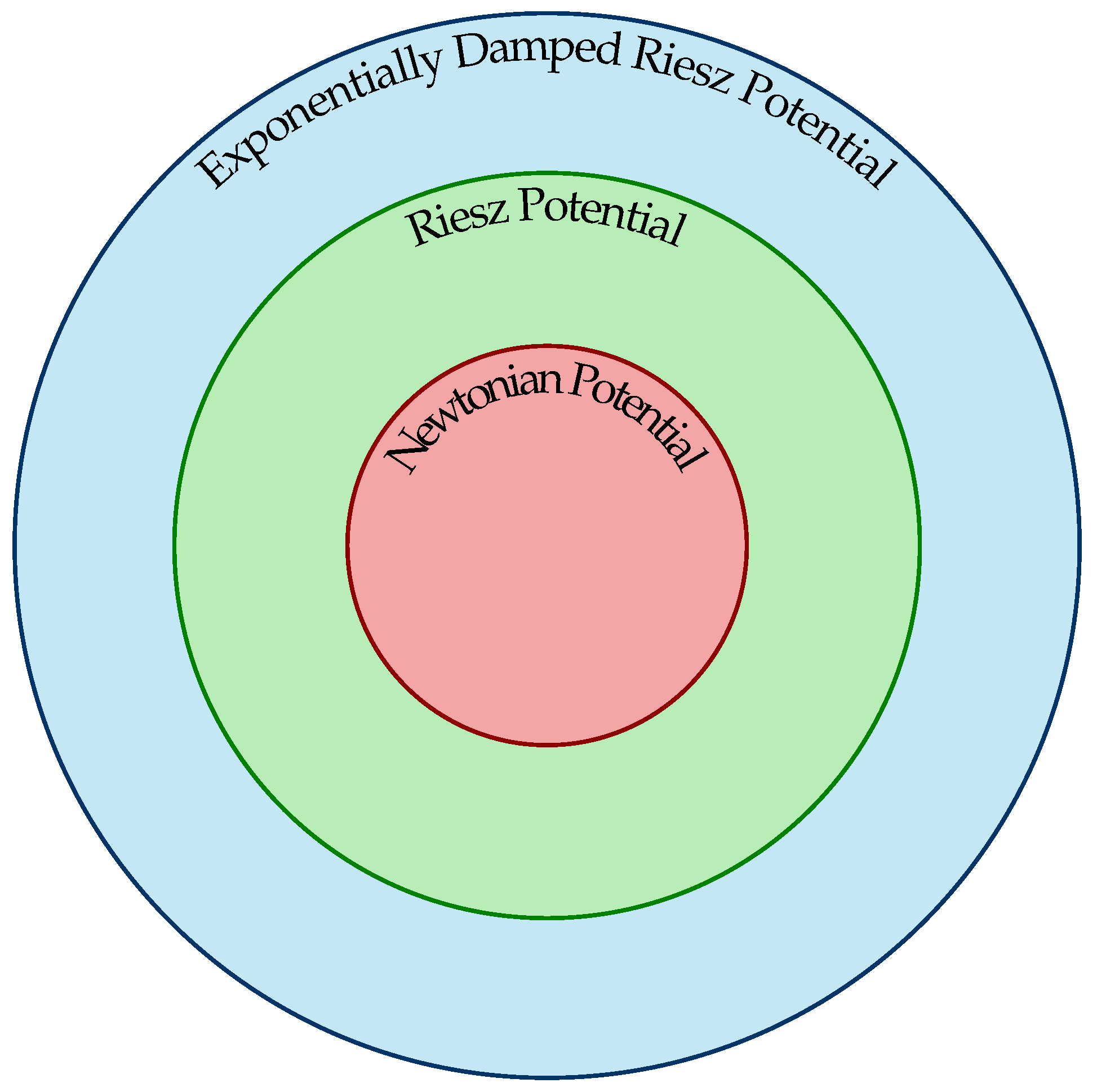
Exponentially Damped Riesz-Type Fractional Integral Operator

Definition 4.

Let $0<\mathsf{\eta }<\mathtt{n}$ and $\mathsf{\beta }\ge 0$. The fractional exponential-type damped integral operator, denoted by ${\mathcal{I}}_{\mathsf{\eta },\mathsf{\beta }}$, is defined as the convolution of a function $\psi \in L_{\mathrm{loc}}^{\mathtt{p}(·)}\left({\mathbf{R}}^{\mathtt{n}}\right)$ with an exponentially damped Riesz-type kernel:

$$\left({\mathcal{I}}_{\mathsf{\eta },\mathsf{\beta }}*\psi \right)(\mu ):={\int }_{{\mathbf{R}}^{\mathtt{n}}}{\displaystyle \frac{\psi (\nu )}{{|\mu -\nu |}^{\mathtt{n}-\mathsf{\eta }}}}{e}^{-\mathsf{\beta }|\mu -\nu |}\mathtt{d}\nu ,$$

where $\mathsf{\eta }$ denotes the order of the fractional operator and $\mathsf{\beta }\ge 0$ controls the exponential decay. For $\mathsf{\beta }=0$, the operator coincides with the classical Riesz potential.

Remark 1.

• When $\mathsf{\beta }=0$ and $\mathsf{\eta }=2$, the operator defined in Definition 4 reduces to

  $${\mathcal{I}}_2\psi (\mu )=c_{\mathtt{n}}{\int }_{{\mathbf{R}}^{\mathtt{n}}}{\displaystyle \frac{\psi (\nu )}{{|\mu -\nu |}^{\mathtt{n}-2}}}\mathtt{d}\nu ,$$

  where $c_{\mathtt{n}}={\displaystyle \frac{1}{(\mathtt{n}-2){\omega }_{\mathtt{n}}}}$, with ${\omega }_{\mathtt{n}}$ being the surface measure of the unit sphere in ${\mathbf{R}}^{\mathtt{n}}$. This is the classical Newtonian potential, which satisfies

  $$-\Delta ({\mathcal{I}}_2\psi )(\mu )=\psi (\mu )$$

  in the distributional sense. For a detailed treatment, see Stein [48]. In portions of the paper where scaling is not central, we adopt $c_{\mathtt{n}}=1$ for simplicity.
• When the exponential decay factor $\mathsf{\beta }=0$, we recover the classical Riesz potential:

  $$\left({\mathcal{I}}_{\mathsf{\eta }}*\psi \right)(\mu ):={\int }_{{\mathbf{R}}^{\mathtt{n}}}{\displaystyle \frac{\psi (\nu )}{{|\mu -\nu |}^{\mathtt{n}-\mathsf{\eta }}}}\mathtt{d}\nu ,$$

  as defined in [48].

The figure below (Figure 1) illustrates the hierarchical structure and the relationships among various classical potentials associated with this new operator.

Novelty and Significance of the Operator

A Specific Example Distinguishing the Operator ${\mathcal{I}}_{\mathsf{\eta },\mathsf{\beta }}$:

Example 2.

Consider the fractional exponential-type damped Riesz operator defined by

$$\left({\mathcal{I}}_{\mathsf{\eta },\mathsf{\beta }}*\psi \right)(\mu ):={\int }_{{\mathbf{R}}^{\mathtt{n}}}{\displaystyle \frac{\psi (\nu )}{{|\mu -\nu |}^{\mathtt{n}-\mathsf{\eta }}}}{e}^{-\mathsf{\beta }|\mu -\nu |}\mathtt{d}\nu ,$$

for $0<\mathsf{\eta }<\mathtt{n}$ and $\mathsf{\beta }>0$. We construct a function $\psi$ for which this operator is well-defined pointwise.

Choice of function. Let

$$\psi (\mu ):={\displaystyle \frac{{\chi }_{\mathcal{B}{(0,1)}^c}(\mu )}{(log(e+{|\mu |\left)\right)}^{\mathtt{p}}}},\mathtt{p}>{\displaystyle \frac{\mathtt{n}-\mathsf{\eta }}{\mathsf{\beta }}}.$$

This decay condition ensures that the function $\psi$ is sufficiently integrable at infinity for the operator to be bounded.

Boundedness under the operator ${\mathcal{I}}_{\mathsf{\eta },\mathsf{\beta }}$. For all $\mu \in {\mathbf{R}}^{\mathtt{n}}$, the following estimate holds:

$$\left|{\mathcal{I}}_{\mathsf{\eta },\mathsf{\beta }}*\psi (\mu )\right|\le {\int }_{{\mathbf{R}}^{\mathtt{n}}}{\displaystyle \frac{e^{-\mathsf{\beta }|\mu -\nu |}}{{|\mu -\nu |}^{\mathtt{n}-\mathsf{\eta }}(log(e+{|\nu |\left)\right)}^{\mathtt{p}}}}\mathtt{d}\nu .$$

Thanks to the imposed condition $\mathtt{p}>{\displaystyle \frac{\mathtt{n}-\mathsf{\eta }}{\mathsf{\beta }}}$, this integral converges due to the dominating exponential decay of the kernel.

Limitation of the classical Riesz and Bessel–Riesz potentials. When the exponential decay is absent (i.e., $\mathsf{\beta }=0$), the kernel reduces to the classical Riesz form:

$${|\mu -\nu |}^{\mathsf{\eta }-\mathtt{n}},$$

and the associated integral

$${\int }_{|\nu |>\mathtt{R}}{\displaystyle \frac{1}{{|\nu |}^{\mathtt{n}-\mathsf{\eta }}(log(e+{|\nu |\left)\right)}^{\mathtt{p}}}}\mathtt{d}\nu$$

may diverge for moderate values of $\mathtt{p}$. In particular, convergence typically requires $\mathtt{p}>1$, indicating a limitation in applying the classical Riesz potential to such slowly decaying functions.

Remark 2.

The function

$$\psi (\mu )={\displaystyle \frac{{\chi }_{\mathcal{B}{(0,1)}^c}(\mu )}{(log(e+{|\mu |\left)\right)}^{\mathtt{p}}}}$$

belongs to the domain of the exponentially damped Riesz operator ${\mathcal{I}}_{\mathsf{\eta },\mathsf{\beta }}$ provided that

$$\mathtt{p}>{\displaystyle \frac{\mathtt{n}-\mathsf{\eta }}{\mathsf{\beta }}}.$$

This ensures sufficient decay of the function at infinity to maintain integrability of the kernel. In contrast, the classical Riesz and Bessel–Riesz operators may be subject to stricter decay requirements on $\psi$, which limits their applicability in certain cases. This highlights the enhanced flexibility and regularizing power of the exponentially damped operator.

First of all, in order to establish the validity of this operator, we have investigated several of its structural properties, which are subsequently utilized in the derivation of the main result. In view of conditions (1) and (2), and taking into account the framework established by Diening [49], a similar type of result was obtained for the Hardy–Littlewood maximal operator.

Lemma 1.

Let $\psi$ be a measurable function taking values in the interval $[0,1]$ on ${\mathbf{R}}^{\mathtt{n}}$, i.e., $\psi :{\mathbf{R}}^{\mathtt{n}}\to [0,1]$, satisfying the following properties:

$$\psi =0\mathrm{almost}\mathrm{everywhere}\mathrm{on}\mathrm{the}\mathrm{ball}\mathcal{B}(0,2{\mathsf{\kappa }}_0),\mathrm{and}{\parallel \psi \parallel }_{\mathtt{p}(·)}\le 1,$$

where the norm is taken with respect to the variable exponent Lebesgue space $L^{\mathtt{p}(·)}\left({\mathbf{R}}^{\mathtt{n}}\right)$, and the exponent function $\mathtt{p}(·)$ satisfies the standard log-Hölder continuity and boundedness conditions. Then the exponential-type fractional integral operator

$${\mathcal{I}}_{\mathsf{\eta },\lambda }\psi (\mu ):={\int }_{{\mathbf{R}}^{\mathtt{n}}}{\displaystyle \frac{\psi (\nu )}{{|\mu -\nu |}^{\mathtt{n}-\mathsf{\eta }}}}{e}^{-\lambda |\mu -\nu |}\mathtt{d}\nu$$

satisfies the inequality

$${\int }_{\mathcal{B}(0,{\mathsf{\kappa }}_0)}{\left[{\mathcal{I}}_{\mathsf{\eta },\lambda }\psi (\mu )\right]}^{\mathtt{p}(\mu )}\mathtt{d}\mu \le \mathcal{C},$$

where $\mathcal{C}$ is a constant depending only on $\mathtt{n},\mathsf{\eta },\lambda ,\mathtt{p}(·),{\mathsf{\kappa }}_0$, and not on $\psi$.

Proof. 

Let $\mu \in \mathcal{B}(0,{\mathsf{\kappa }}_0)$. Since $\psi (\nu )=0$ on $\mathcal{B}(0,2{\mathsf{\kappa }}_0)$, it follows that $|\nu |\ge 2{\mathsf{\kappa }}_0$ wherever $\psi (\nu )\ne 0$, and hence,

$$|\mu -\nu |\ge |\nu |-|\mu |\ge 2{\mathsf{\kappa }}_0-{\mathsf{\kappa }}_0={\mathsf{\kappa }}_0.$$

Therefore,

$${\mathcal{I}}_{\mathsf{\eta },\lambda }\psi (\mu )\le {\int }_{|\nu |\ge 2{\mathsf{\kappa }}_0}{\displaystyle \frac{\psi (\nu )}{{|\mu -\nu |}^{\mathtt{n}-\mathsf{\eta }}}}{e}^{-\lambda |\mu -\nu |}\mathtt{d}\nu \le {\mathcal{C}}_{{\mathsf{\kappa }}_0,\lambda }{\int }_{|\nu |\ge 2{\mathsf{\kappa }}_0}\psi (\nu )\mathtt{d}\nu .$$

Since $\psi (\nu )\in [0,1]$ and ${\parallel \psi \parallel }_{\mathtt{p}(·)}\le 1$, we use the modular inequality

$${\int }_{{\mathbf{R}}^{\mathtt{n}}}\psi (\nu )\mathtt{d}\nu \le {\int }_{{\mathbf{R}}^{\mathtt{n}}}\psi {(\nu )}^{\mathtt{p}(\nu )}\mathtt{d}\nu \le 1.$$

Thus,

$${\mathcal{I}}_{\mathsf{\eta },\lambda }\psi (\mu )\le \mathcal{M}\mathrm{for}\mathrm{all}\mu \in \mathcal{B}(0,{\mathsf{\kappa }}_0),$$

where $\mathcal{M}$ depends only on ${\mathsf{\kappa }}_0,\lambda$, and $\mathtt{n}$.

Now we estimate

$${\int }_{\mathcal{B}(0,{\mathsf{\kappa }}_0)}{\left[{\mathcal{I}}_{\mathsf{\eta },\lambda }\psi (\mu )\right]}^{\mathtt{p}(\mu )}\mathtt{d}\mu \le {\int }_{\mathcal{B}(0,{\mathsf{\kappa }}_0)}{\mathcal{M}}^{\mathtt{p}(\mu )}\mathtt{d}\mu \le \mathcal{C}.$$

Note: Since $\psi \in [0,1]\subset L^{\infty }\left({\mathbb{R}}^n\right)\cap L^{\mathtt{p}(·)}\left({\mathbb{R}}^n\right)$, and the exponent function $\mathtt{p}(·)$ is log-Hölder continuous and essentially bounded, both the integral and modular expressions are well-defined. The change in the order of integration is justified by Fubini-type theorems adapted to variable exponent spaces (cf. Diening et al., 2011 [16]). Therefore, no issues arise concerning measurability or integrability.

This concludes the proof. □

Lemma 2.

Let $\psi$ be a measurable function taking values in the interval $[0,1]$ on ${\mathbf{R}}^{\mathtt{n}}$, that is, $\psi :{\mathbf{R}}^{\mathtt{n}}\to [0,1]$, such that

$$\psi =0\mathrm{on}\mathcal{B}(0,2{\mathsf{\kappa }}_0),\mathrm{and}{\parallel \psi \parallel }_{\mathtt{p}(·)}\le 1.$$

Then the exponential-type fractional integral operator

$${\mathcal{I}}_{\mathsf{\eta },\lambda }\psi (\mu ):={\int }_{{\mathbf{R}}^{\mathtt{n}}}{\displaystyle \frac{\psi (\nu )}{{|\mu -\nu |}^{\mathtt{n}-\mathsf{\eta }}}}{e}^{-\lambda |\mu -\nu |}\mathtt{d}\nu$$

satisfies

$${\int }_{\mathcal{B}(0,{\mathsf{\kappa }}_0)}{\left[{\mathcal{I}}_{\mathsf{\eta },\lambda }\psi (\mu )\right]}^{\mathtt{p}(\mu )}\mathtt{d}\mu \le \mathcal{C},$$

where $\mathcal{C}$ is a constant depending only on $\mathtt{n},\mathsf{\eta },\lambda ,\mathtt{p}(·),{\mathsf{\kappa }}_0$, but not on $\psi$.

Proof. 

Let $\mu \in \mathcal{B}(0,{\mathsf{\kappa }}_0)$. Since $\psi =0$ on $\mathcal{B}(0,2{\mathsf{\kappa }}_0)$, it follows that if $\nu \in supp(\psi )$, then $|\nu |\ge 2{\mathsf{\kappa }}_0$. Here, the support of the function $\psi$, denoted by $supp(\psi )$, is defined as the closure of the set where $\psi$ is nonzero, i.e.,

$$supp(\psi ):=\overline{\{\nu \in {\mathbf{R}}^{\mathtt{n}}:\psi (\nu )\ne 0\}}.$$

Thus, since $\mu \in \mathcal{B}(0,{\mathsf{\kappa }}_0)$ and every point in $supp(\psi )$ lies outside the ball $\mathcal{B}(0,2{\mathsf{\kappa }}_0)$, it follows that $|\mu -\nu |\ge {\mathsf{\kappa }}_0$. Therefore,

$${\mathcal{I}}_{\mathsf{\eta },\lambda }\psi (\mu )\le {\int }_{{\mathbf{R}}^{\mathtt{n}}\setminus \mathcal{B}(0,2{\mathsf{\kappa }}_0)}{\displaystyle \frac{\psi (\nu )}{{\mathsf{\kappa }}_0^{\mathtt{n}-\mathsf{\eta }}}}{e}^{-\lambda {\mathsf{\kappa }}_0}\mathtt{d}\nu ={\displaystyle \frac{e^{-\lambda {\mathsf{\kappa }}_0}}{{\mathsf{\kappa }}_0^{\mathtt{n}-\mathsf{\eta }}}}\int \psi (\nu )\mathtt{d}\nu .$$

Since $\psi (\nu )\in [0,1]$ and ${\parallel \psi \parallel }_{\mathtt{p}(·)}\le 1$, we obtain

$${\int }_{{\mathbf{R}}^{\mathtt{n}}}\psi (\nu )\mathtt{d}\nu \le {\int }_{{\mathbf{R}}^{\mathtt{n}}}\psi {(\nu )}^{\mathtt{p}(\nu )}\mathtt{d}\nu \le 1.$$

Hence,

$${\mathcal{I}}_{\mathsf{\eta },\lambda }\psi (\mu )\le \mathcal{M}\mathrm{for}\mathrm{all}\mu \in \mathcal{B}(0,{\mathsf{\kappa }}_0),$$

for some constant $\mathcal{M}$ depending only on the fixed parameters.

It follows that

$${\int }_{\mathcal{B}(0,{\mathsf{\kappa }}_0)}{\left[{\mathcal{I}}_{\mathsf{\eta },\lambda }\psi (\mu )\right]}^{\mathtt{p}(\mu )}\mathtt{d}\mu \le {\int }_{\mathcal{B}(0,{\mathsf{\kappa }}_0)}{\mathcal{M}}^{\mathtt{p}(\mu )}\mathtt{d}\mu \le \mathcal{C},$$

which completes the proof. □

Before proving the lemma below, we define the Hardy operator, which will be used in the sequel:

$$\mathcal{M}\psi (\nu ):={\displaystyle \frac{1}{\left|\mathcal{B}\right(0,|\nu |\left)\right|}}{\int }_{\mathcal{B}(0,|x\left|\right)}|\psi (\mu )|\mathtt{d}\mu ,$$

where $\mathcal{B}(0,|\nu \left|\right)$ denotes the ball centered at the origin with radius $|\nu |$, and $\left|\mathcal{B}\right(0,|\nu |\left)\right|$ is its Lebesgue measure.

Lemma 3.

Let $\psi$ be a measurable function on ${\mathbf{R}}^{\mathtt{n}}$ taking values in the set of non-negative extended real numbers, i.e., $\psi :{\mathbf{R}}^{\mathtt{n}}\to [0,\infty )$, such that $\psi =0$ on the ball $\mathcal{B}(0,{\mathsf{\kappa }}_0)$, and moreover, it satisfies the modular constraint ${\parallel \psi \parallel }_{\mathtt{p}(·)}\le 1$. Define the exponentially damped Riesz-type operator by

$$\left({\mathcal{I}}_{\mathsf{\eta },\lambda }*\psi \right)(\mu ):={\int }_{{\mathbf{R}}^{\mathtt{n}}}{\displaystyle \frac{\psi (\nu )}{{|\mu -\nu |}^{\mathtt{n}-\mathsf{\eta }}}}{e}^{-\lambda |\mu -\nu |}\mathtt{d}\nu ,\mu \in {\mathbf{R}}^{\mathtt{n}},|\mu |>{\mathsf{\kappa }}_0.$$

Then, for all $\mu \in {\mathbf{R}}^{\mathtt{n}}$ with $|\mu |\ge {\mathsf{\kappa }}_0$, it holds that

$$\left({\mathcal{I}}_{\mathsf{\eta },\lambda }*\psi \right)(\mu )\le \mathcal{C}exp\left({\left({\displaystyle \frac{1}{\left|\mathcal{B}\right(0,|\mu |\left)\right|}}{\int }_{\mathcal{B}(0,|\mu \left|\right)}\psi {(\nu )}^{\mathtt{p}(\nu )}\mathtt{d}\nu \right)}^{1/\mathtt{p}(\mu )}\right),$$

where $\mathcal{C}>0$ is a constant independent of $\psi$ and $\mu$.

Proof. 

Let $\psi \in L^{\mathtt{p}(·)}\left({\mathbf{R}}^{\mathtt{n}}\right)$ be a measurable function taking values in the set of non-negative real numbers, i.e., $\psi (\xi )\ge 0$ for almost every $\xi \in {\mathbf{R}}^{\mathtt{n}}$, such that $\psi =0$ on the ball $\mathcal{B}(0,{\mathsf{\kappa }}_0)$ and ${\parallel \psi \parallel }_{\mathtt{p}(·)}\le 1$. Define

$$\mathbf{F}:={\displaystyle \frac{1}{\left|\mathcal{B}\right(0,|\mu |\left)\right|}}{\int }_{\mathcal{B}(0,|\mu \left|\right)}\psi {(\nu )}^{\mathtt{p}(\nu )}\mathtt{d}\nu .$$

Since $\psi =0$ on $\mathcal{B}(0,{\mathsf{\kappa }}_0)$, the kernel ${|\mu -\nu |}^{\mathsf{\eta }-\mathtt{n}}{e}^{-\lambda |\mu -\nu |}$ decays rapidly. Thus, the dominant contribution to the integral arises from $\nu \in \mathcal{B}(0,|\mu \left|\right)\setminus \mathcal{B}(0,{\mathsf{\kappa }}_0)$.

We use Hölder’s inequality with exponent $\mathtt{q}(\nu ):=\mathtt{p}(\nu )$, so ${\mathtt{q}}^{\prime }(\nu ):={\displaystyle \frac{\mathtt{p}(\nu )}{\mathtt{p}(\nu )-1}}$, to estimate

$$\begin{array}{cc}\hfill \left({\mathcal{I}}_{\mathsf{\eta },\lambda }*\psi \right)(\mu )& ={\int }_{{\mathrm{R}}^{\mathtt{n}}}{\displaystyle \frac{\psi (\nu )}{{|\mu -\nu |}^{\mathtt{n}-\mathsf{\eta }}}}{e}^{-\lambda |\mu -\nu |}\mathtt{d}\nu \hfill \\ & \le {\int }_{\mathcal{B}(0,|\mu \left|\right)}{\displaystyle \frac{\psi (\nu )}{{|\mu -\nu |}^{\mathtt{n}-\mathsf{\eta }}}}{e}^{-\lambda |\mu -\nu |}\mathtt{d}\nu \hfill \\ & \le {\left({\int }_{\mathcal{B}(0,|\mu \left|\right)}{\left[{\displaystyle \frac{1}{{|\mu -\nu |}^{\mathtt{n}-\mathsf{\eta }}}}{e}^{-\lambda |\mu -\nu |}\right]}^{{\mathtt{q}}^{\prime }(\nu )}\mathtt{d}\nu \right)}^{1/{\mathtt{q}}^{\prime }(\mu )}·{\mathbf{F}}^{1/\mathtt{p}(\mu )}.\hfill \end{array}$$

Since the kernel is integrable over ${\mathbf{R}}^{\mathtt{n}}$ for $0<\mathsf{\eta }<\mathtt{n}$, and the exponential term ensures decay, the integral is bounded. Thus, we obtain

$$\left({\mathcal{I}}_{\mathsf{\eta },\lambda }*\psi \right)(\mu )\le \mathcal{C}·exp\left({\mathbf{F}}^{1/\mathtt{p}(\mu )}\right),$$

for some constant $\mathcal{C}>0$ depending only on $\mathtt{n},\mathsf{\eta },\lambda$, and the modular exponent $\mathtt{p}(·)$, but not on $\psi$ or $\mu$. This completes the proof. □

Theorem 5.

Let $0<\mathsf{\eta }<\mathtt{n}$, $0<\gamma <\infty$ with $\mathsf{\eta }<\gamma$, and suppose that $\mathtt{p}(·)\in {\mathbf{P}}_0^{log}(\Omega )\left({\mathbf{R}}^{+}\right)$, i.e., the exponent function satisfies the log-Hölder continuity condition. Then, the fractional integral operator with exponential-type kernel

$${\mathcal{I}}_{\mathsf{\eta },\mathsf{\beta }}\psi (\mu ):={\int }_{{\mathbf{R}}^{\mathbf{n}}}{\displaystyle \frac{\psi (\nu )}{{|\mu -\nu |}^{\mathtt{n}-\mathsf{\eta }}}}{e}^{-\mathsf{\beta }|\mu -\nu |}\mathtt{d}\nu$$

is bounded on the variable exponent Lebesgue space $L^{\mathtt{p}(·)}\left({\mathbf{R}}^{+}\right)$, i.e.,

$${\mathcal{I}}_{\mathsf{\eta },\mathsf{\beta }}:L^{\mathtt{p}(·)}\left({\mathbf{R}}^{+}\right)\to L^{\mathtt{p}(·)}\left({\mathbf{R}}^{+}\right)$$

is a bounded operator.

Proof. 

Since the essential supremum ${\mathtt{p}}_{+}<\infty$ and the exponent function $\mathtt{p}(·)$ satisfies the log-Hölder continuity condition, i.e., $\mathtt{p}(·)\in {\mathbf{P}}_0^{log}(\Omega )\left({\mathbf{R}}^{+}\right)$, it follows that the Hardy–Littlewood maximal operator $\mathcal{M}$ is bounded on the variable exponent Lebesgue space $L^{\mathtt{p}(·)}\left({\mathbf{R}}^{+}\right)$. More precisely, there exists a constant $c_0>0$ such that for every $\psi \in L^{\mathtt{p}(·)}\left({\mathrm{R}}^{+}\right)$, we have

$${\parallel \mathcal{M}\psi \parallel }_{L^{\mathtt{p}(·)}\left({\mathbf{R}}^{+}\right)}\le c_0{\parallel \psi \parallel }_{L^{\mathtt{p}(·)}\left({\mathbf{R}}^{+}\right)}.$$

Now, fix any $\mu \in {\mathbf{R}}^{+}$ and let $\psi \in L^{\mathtt{p}(·)}\left({\mathbf{R}}^{+}\right)$. Consider the fractional integral operator with exponential kernel defined by

$${\mathcal{I}}_{\mathsf{\eta },\mathsf{\beta }}\psi (\mu ):={\int }_{{\mathbf{R}}^{\mathtt{n}}}{\displaystyle \frac{\psi (\nu )}{{|\mu -\nu |}^{\mathtt{n}-\mathsf{\eta }}}}{e}^{-\mathsf{\beta }|\mu -\nu |}\mathtt{d}\nu .$$

To facilitate estimation, we split the integral into two parts based on the distance between $\mu$ and $\nu$:

$${\mathcal{I}}_{\mathsf{\eta },\mathsf{\beta }}\psi (\mu )=\underset{:={\mathfrak{I}}_1(\mu )}{\underbrace{{\int }_{|\mu -\nu |<1}{\displaystyle \frac{\psi (\nu )}{{|\mu -\nu |}^{\mathtt{n}-\mathsf{\eta }}}}{e}^{-\mathsf{\beta }|\mu -\nu |}\mathtt{d}\nu }}+\underset{:={\mathfrak{I}}_2(\mu )}{\underbrace{{\int }_{|\mu -\nu |\ge 1}{\displaystyle \frac{\psi (\nu )}{{|\mu -\nu |}^{\mathtt{n}-\mathsf{\eta }}}}{e}^{-\mathsf{\beta }|\mu -\nu |}\mathtt{d}\nu }}.$$

Now, fix any $\mu \in {\mathbf{R}}^{+}$ and let $\psi \in L^{\mathtt{p}(·)}\left({\mathbf{R}}^{+}\right)$. To estimate the local part of the fractional potential operator, we begin by decomposing the unit ball centered at $\mu \in {\mathbf{R}}^{\mathbf{n}}$, defined by

$$\mathcal{B}(\mu ,1):=\left\{\nu \in {\mathbf{R}}^{\mathbf{n}}:|\mu -\nu |<1\right\},$$

into a countable union of dyadic annuli, which facilitates control over the singularity and decay behavior of the kernel.

The dyadic annuli are given by

$${\mathcal{A}}_{\mathtt{k}}:=\left\{\nu \in {\mathbf{R}}^{\mathbf{n}}:2^{\mathtt{k}}\le |\mu -\nu |<2^{\mathtt{k}+1}\right\},\mathrm{for}\mathtt{k}\le -1.$$

These sets are pairwise disjoint, and their union covers the unit ball:

$$\mathcal{B}(\mu ,1)=\bigcup _{\mathtt{k}=-\infty }^{-1}{\mathcal{A}}_{\mathtt{k}},(\mathrm{disjoint}\mathrm{union}).$$

Hence, the local integral

$${\mathcal{I}}_1(\mu ):={\int }_{|\mu -\nu |<1}{\displaystyle \frac{|\psi (\nu \left)\right|}{{|\mu -\nu |}^{\mathtt{n}-\mathsf{\eta }}}}{e}^{-\mathsf{\beta }|\mu -\nu |}\mathtt{d}\nu$$

can be estimated by summing over the dyadic annuli:

$${\mathcal{I}}_1(\mu )\le \sum _{\mathtt{k}=-\infty }^{-1}{\int }_{{\mathcal{A}}_{\mathtt{k}}}{\displaystyle \frac{|\psi (\nu \left)\right|}{{|\mu -\nu |}^{\mathtt{n}-\mathsf{\eta }}}}{e}^{-\mathsf{\beta }|\mu -\nu |}\mathtt{d}\nu .$$

Since $|\mu -\nu |<1$ for all $\nu \in {\mathcal{A}}_{\mathtt{k}}$, we observe that $e^{-\mathsf{\beta }|\mu -\nu |}\le 1$. Therefore,

$${\mathcal{I}}_1(\mu )\le \sum _{\mathtt{k}=-\infty }^{-1}{\int }_{{\mathcal{A}}_{\mathtt{k}}}{\displaystyle \frac{|\psi (\nu \left)\right|}{{|\mu -\nu |}^{\mathtt{n}-\mathsf{\eta }}}}\mathtt{d}\nu .$$

On each annulus ${\mathcal{A}}_{\mathtt{k}}$, we have the estimate $|\mu -\nu |\sim 2^{\mathtt{k}}$, so we may write

$${\int }_{{\mathcal{A}}_{\mathtt{k}}}{\displaystyle \frac{|\psi (\nu \left)\right|}{{|\mu -\nu |}^{\mathtt{n}-\mathsf{\eta }}}}\mathtt{d}\nu \le {\displaystyle \frac{1}{{\left(2^{\mathtt{k}}\right)}^{\mathtt{n}-\mathsf{\eta }}}}{\int }_{{\mathcal{A}}_{\mathtt{k}}}|\psi (\nu )|\mathtt{d}\nu .$$

Using the volume estimate for balls and the definition of the Hardy–Littlewood maximal function, we obtain

$${\int }_{{\mathcal{A}}_{\mathtt{k}}}|\psi (\nu )|\mathtt{d}\nu \le |\mathcal{B}(\mu ,2^{\mathtt{k}+1})|·\mathcal{M}\psi (\mu )\le {\mathcal{C}}_{\mathtt{n}}·2^{\mathtt{k}\mathtt{n}}·\mathcal{M}\psi (\mu ),$$

where ${\mathcal{C}}_{\mathtt{n}}=\left|\mathcal{B}(0,1)\right|·2^{\mathtt{n}}$ is a dimensional constant.

Combining the above inequalities yields

$${\int }_{{\mathcal{A}}_{\mathtt{k}}}{\displaystyle \frac{|\psi (\nu \left)\right|}{{|\mu -\nu |}^{\mathtt{n}-\mathsf{\eta }}}}\mathtt{d}\nu \le {\mathcal{C}}_{\mathtt{n}}·{\displaystyle \frac{2^{\mathtt{k}\mathtt{n}}}{2^{\mathtt{k}(\mathtt{n}-\mathsf{\eta })}}}·\mathcal{M}\psi (\mu )={\mathcal{C}}_{\mathtt{n}}·2^{\mathtt{k}\mathsf{\eta }}·\mathcal{M}\psi (\mu ).$$

Summing over all $\mathtt{k}\le -1$, we obtain

$${\mathcal{I}}_1(\mu )\le {\mathcal{C}}_{\mathtt{n}}·\mathcal{M}\psi (\mu )\sum _{\mathtt{k}=-\infty }^{-1}{2}^{\mathtt{k}\mathsf{\eta }}={\mathcal{C}}_1·\mathcal{M}\psi (\mu ),$$

where

$${\mathcal{C}}_1:={\mathcal{C}}_{\mathtt{n}}\sum _{\mathtt{k}=-\infty }^{-1}{2}^{\mathtt{k}\mathsf{\eta }}={\mathcal{C}}_{\mathtt{n}}·{\displaystyle \frac{2^{-\mathsf{\eta }}}{1-2^{-\mathsf{\eta }}}},$$

since the geometric series converges for $\mathsf{\eta }>0$. This completes the estimate for the local term ${\mathcal{I}}_1(\mu )$.

Now, we consider the global component of the regularized fractional integral operator:

$${\mathcal{I}}_2(\mu )={\int }_{|\mu -\nu |\ge 1}{\displaystyle \frac{\psi (\nu )}{{|\mu -\nu |}^{\mathtt{n}-\mathsf{\eta }}}}{e}^{-\mathsf{\beta }|\mu -\nu |}\mathtt{d}\nu ,$$

where $0<\mathsf{\eta }<\mathtt{n}$, $\mathsf{\beta }>0$, and $\psi \in L_{\mathrm{loc}}^1\left({\mathbf{R}}^{\mathtt{n}}\right)$. Our goal is to estimate this term in terms of the Hardy–Littlewood maximal function $\mathcal{M}\psi (\mu )$.

We decompose the domain of integration into dyadic annuli:

$${\mathcal{I}}_2(\mu )\le \sum _{\mathtt{k}=0}^{\infty }{\int }_{2^{\mathtt{k}}\le |\mu -\nu |<2^{\mathtt{k}+1}}{\displaystyle \frac{|\psi (\nu \left)\right|}{{|\mu -\nu |}^{\mathtt{n}-\mathsf{\eta }}}}{e}^{-\mathsf{\beta }|\mu -\nu |}\mathtt{d}\nu .$$

For each fixed $\mathtt{k}\ge 0$, and $\nu \in {\mathbf{R}}^{\mathtt{n}}$ such that $2^{\mathtt{k}}\le |\mu -\nu |<2^{\mathtt{k}+1}$, we observe

$$\begin{array}{cc}\hfill e^{-\mathsf{\beta }|\mu -\nu |}& \le e^{-\mathsf{\beta }{2}^{\mathtt{k}}},\hfill \\ \hfill {|\mu -\nu |}^{-(\mathtt{n}-\mathsf{\eta })}& \le {\left(2^{\mathtt{k}}\right)}^{-(\mathtt{n}-\mathsf{\eta })}.\hfill \end{array}$$

Hence,

$${\int }_{2^{\mathtt{k}}\le |\mu -\nu |<2^{\mathtt{k}+1}}{\displaystyle \frac{|\psi (\nu \left)\right|}{{|\mu -\nu |}^{\mathtt{n}-\mathsf{\eta }}}}{e}^{-\mathsf{\beta }|\mu -\nu |}\mathtt{d}\nu \le e^{-\mathsf{\beta }{2}^{\mathtt{k}}}·{\displaystyle \frac{1}{2^{\mathtt{k}(\mathtt{n}-\mathsf{\eta })}}}{\int }_{2^{\mathtt{k}}\le |\mu -\nu |<2^{\mathtt{k}+1}}|\psi (\nu )|\mathtt{d}\nu .$$

Now, the measure of the annular region satisfies

$$\left|\left\{\nu \in {\mathrm{R}}^{\mathrm{n}}:2^{\mathtt{k}}\le |\mu -\nu |<2^{\mathtt{k}+1}\right\}\right|\le {\mathtt{C}}_{\mathtt{n}}·2^{\mathtt{k}\mathtt{n}},$$

and the integral over the annulus can be estimated using the maximal function:

$${\int }_{2^{\mathtt{k}}\le |\mu -\nu |<2^{\mathtt{k}+1}}|\psi (\nu )|\mathtt{d}\nu \le {\int }_{\mathcal{B}(\mu ,2^{\mathtt{k}+1})}|\psi (\nu )|\mathtt{d}\nu \le \mathcal{C}·2^{\mathtt{k}\mathtt{n}}·\mathcal{M}\psi (\mu ).$$

Therefore, each dyadic term is bounded by

$${\int }_{2^{\mathtt{k}}\le |\mu -\nu |<2^{\mathtt{k}+1}}{\displaystyle \frac{|\psi (\nu \left)\right|}{{|\mu -\nu |}^{\mathtt{n}-\mathsf{\eta }}}}{e}^{-\mathsf{\beta }|\mu -\nu |}\mathtt{d}\nu \le \mathcal{C}·2^{\mathtt{k}\mathsf{\eta }}{e}^{-\mathsf{\beta }{2}^{\mathtt{k}}}·\mathcal{M}\psi (\mu ).$$

Summing over all dyadic shells gives

$${\mathcal{I}}_2(\mu )\le \mathcal{C}·\mathcal{M}\psi (\mu )\sum _{\mathtt{k}=0}^{\infty }{2}^{\mathtt{k}\mathsf{\eta }}{e}^{-\mathsf{\beta }{2}^{\mathtt{k}}}.$$

Since $e^{-\mathsf{\beta }{2}^{\mathtt{k}}}$ decays faster than any polynomial growth of $2^{\mathtt{k}\mathsf{\eta }}$, the sum converges:

$$\sum _{\mathtt{k}=0}^{\infty }{2}^{\mathtt{k}\mathsf{\eta }}{e}^{-\mathsf{\beta }{2}^{\mathtt{k}}}<\infty .$$

Thus, we conclude

$${\mathcal{I}}_2(\mu )\le {\mathcal{C}}_2·\mathcal{M}\psi (\mu ),$$

where ${\mathcal{C}}_2>0$ depends only on $\mathtt{n},\mathsf{\eta },\mathsf{\beta }$.

Combining the local and global estimates,

$${\mathcal{I}}_{\mathsf{\eta },\mathsf{\beta }}\psi (\mu )={\mathcal{I}}_1(\mu )+{\mathcal{I}}_2(\mu )\le \mathcal{C}·\mathcal{M}\psi (\mu ).$$

Let

$$\mathsf{\beta }\in \left\{\mathsf{\beta }>0:{\rho }_{\mathtt{p}(·)}\left({\displaystyle \frac{\mathcal{M}\psi }{\mathsf{\beta }}}\right)\le 1\right\}.$$

Then we have

$$\left|{\displaystyle \frac{{\mathcal{I}}_{\mathsf{\eta },\mathsf{\beta }}\psi (\mu )/{\mathcal{C}}_3}{\mathsf{\beta }}}\right|\le {\displaystyle \frac{|\mathcal{M}\psi (\mu \left)\right|}{\mathsf{\beta }}}.$$

Applying the modular function ${\rho }_{\mathtt{p}(·)}$, we obtain

$${\rho }_{\mathtt{p}(·)}\left({\displaystyle \frac{{\mathcal{I}}_{\mathsf{\eta },\mathsf{\beta }}\psi /{\mathcal{C}}_3}{\mathsf{\beta }}}\right)\le {\rho }_{\mathtt{p}(·)}\left({\displaystyle \frac{\mathcal{M}\psi }{\mathsf{\beta }}}\right)\le 1.$$

This implies

$$\mathsf{\beta }\in \left\{\mathsf{\beta }>0:{\rho }_{\mathtt{p}(·)}\left({\displaystyle \frac{{\mathcal{I}}_{\mathsf{\eta },\mathsf{\beta }}\psi /{\mathcal{C}}_3}{\mathsf{\beta }}}\right)\le 1\right\}.$$

By the definition of the Luxemburg norm, it follows that

$${∥{\displaystyle \frac{{\mathcal{I}}_{\mathsf{\eta },\mathsf{\beta }}\psi }{{\mathcal{C}}_3}}∥}_{L^{\mathtt{p}(·)}}\le {∥\mathcal{M}\psi ∥}_{L^{\mathtt{p}(·)}}.$$

Using the boundedness of the Hardy–Littlewood maximal operator on variable exponent Lebesgue spaces $L^{\mathtt{p}(·)}$, we get

$${∥\mathcal{M}\psi ∥}_{L^{\mathtt{p}(·)}}\le {\mathtt{c}}_0{∥\psi ∥}_{L^{\mathtt{p}(·)}}.$$

Hence, we conclude

$${∥{\mathcal{I}}_{\mathsf{\eta },\mathsf{\beta }}\psi ∥}_{L^{\mathtt{p}(·)}}\le {\mathcal{C}}_4{∥\psi ∥}_{L^{\mathtt{p}(·)}},$$

where ${\mathcal{C}}_4={\mathcal{C}}_3{\mathtt{c}}_0$. □

Example 3.

Let $0<\mathsf{\eta }<\mathtt{n}$ and $0<\mathsf{\gamma }<\infty$ with $\mathsf{\eta }<\mathsf{\gamma }$. Assume that the exponent function $\mathtt{p}(·)$ belongs to the class ${\mathbf{P}}_0^{log}(\Omega )\left({\mathbf{R}}^{+}\right)$, i.e., it satisfies the log-Hölder continuity condition on ${\mathbf{R}}^{+}$.

For the specific case $\mathtt{n}=1$, $\mathsf{\eta }={\displaystyle \frac{1}{2}}$, and $\mathsf{\gamma }=1$, consider the variable exponent function

$$\mathtt{p}(\mu )=2+{\displaystyle \frac{1}{1+|\mu |}},\mu \in {\mathbf{R}}^{+},$$

which satisfies

$$2\le \mathtt{p}(\mu )\le 3,\mathrm{for}\mathrm{all}\mu \ge 0.$$

We verify that $\mathtt{p}$ satisfies the log-Hölder continuity condition, i.e., there exists a constant $\mathcal{C}>0$ such that for all $\mu ,\nu \in {\mathbf{R}}^{+}$ with $\mu \ne \nu$,

$$|\mathtt{p}(\mu )-\mathtt{p}(\nu )|\le {\displaystyle \frac{\mathcal{C}}{log\left(e+\frac{1}{|\mu -\nu |}\right)}}.$$

Note that

$$|\mathtt{p}(\mu )-\mathtt{p}(\nu )|=\left|{\displaystyle \frac{1}{1+|\mu |}}-{\displaystyle \frac{1}{1+|\nu |}}\right|={\displaystyle \frac{\left|\right|\nu |-|\mu \left|\right|}{(1+|\mu \left|\right)(1+|\nu \left|\right)}}.$$

By the triangle inequality,

$$\left|\right|\mu |-|\nu \left|\right|\le |\mu -\nu |,$$

hence,

$$|\mathtt{p}(\mu )-\mathtt{p}(\nu )|\le {\displaystyle \frac{|\mu -\nu |}{(1+|\mu \left|\right)(1+|\nu \left|\right)}}\le |\mu -\nu |.$$

For $\mathtt{t}:=|\mu -\nu |\in (0,1]$, since the function

$$\psi \left(\mathtt{t}\right)=\mathtt{t}log\left(e+{\displaystyle \frac{1}{\mathtt{t}}}\right)$$

is bounded below by a positive constant, there exists $\mathcal{C}>0$ such that

$$\mathtt{t}\le {\displaystyle \frac{\mathcal{C}}{log\left(e+\frac{1}{\mathtt{t}}\right)}}.$$

Therefore,

$$|\mathtt{p}(\mu )-\mathtt{p}(\nu )|\le {\displaystyle \frac{\mathcal{C}}{log\left(e+\frac{1}{|\mu -\nu |}\right)}}.$$

Thus, $\mathtt{p}$ satisfies the log-Hölder continuity condition on ${\mathbf{R}}^{+}$. Define the fractional integral operator by

$${\mathcal{I}}_{\mathsf{\eta },\gamma }\psi (\mu ):={\int }_0^{\infty }{\displaystyle \frac{\psi (\nu )}{{|\mu -\nu |}^{1-\mathsf{\eta }}}}{e}^{-\gamma |\mu -\nu |}\mathtt{d}\nu ,\mu \in {\mathbf{R}}^{+}.$$

Let $\psi$ be the characteristic function of the interval $[0,1]$, defined by

$$\psi (\nu ):={\chi }_{[0,1]}(\nu )=\left\{\begin{array}{cc}1,\hfill & \nu \in [0,1],\hfill \\ 0,\hfill & \nu \notin [0,1].\hfill \end{array}\right.$$

The Luxemburg norm of $\psi$ in the variable exponent Lebesgue space $L^{\mathtt{p}(·)}\left({\mathbf{R}}^{+}\right)$ is given by

$${\parallel \psi \parallel }_{L^{\mathtt{p}(·)}\left({\mathbf{R}}^{+}\right)}=inf\left\{\mathsf{\beta }>0:{\int }_0^{\infty }{\left|{\displaystyle \frac{\psi (\mu )}{\mathsf{\beta }}}\right|}^{\mathtt{p}(\mu )}\mathtt{d}\mu \le 1\right\}.$$

Since $\psi (\mu )=1$ for $\mu \in [0,1]$ and zero elsewhere,

$${\int }_0^{\infty }{\left|{\displaystyle \frac{\psi (\mu )}{\mathsf{\beta }}}\right|}^{\mathtt{p}(\mu )}\mathtt{d}\mu ={\int }_0^1{\mathsf{\beta }}^{-\mathtt{p}(\mu )}\mathtt{d}\mu .$$

Using the lower bound $\mathtt{p}(\mu )\ge 2$,

$${\int }_0^1{\mathsf{\beta }}^{-\mathtt{p}(\mu )}\mathtt{d}\mu \le {\int }_0^1{\mathsf{\beta }}^{-2}\mathtt{d}\mu ={\mathsf{\beta }}^{-2}.$$

Choosing $\mathsf{\beta }=1$ yields

$${\int }_0^1{1}^{-\mathtt{p}(\mu )}\mathtt{d}\mu \le 1,$$

so

$${\parallel \psi \parallel }_{L^{\mathtt{p}(·)}\left({\mathbf{R}}^{+}\right)}\le 1.$$

For $\mu \in {\mathbf{R}}^{+}$, the operator ${\mathcal{I}}_{\mathsf{\eta },\gamma }\psi (\mu )$ evaluates as

$${\mathcal{I}}_{\mathsf{\eta },\gamma }\psi (\mu )={\int }_0^1{\displaystyle \frac{e^{-|\mu -\nu |}}{{|\mu -\nu |}^{\frac{1}{2}}}}\mathtt{d}\nu .$$

Thus, $\mathtt{p}$ satisfies the log-Hölder continuity condition on ${\mathbf{R}}^{+}$.

When $\mu \ge 2$, we have $|\mu -\nu |\ge 1$, and therefore,

$${\mathcal{I}}_{\mathsf{\eta },\gamma }\psi (\mu )\le {\int }_0^1{\displaystyle \frac{e^{-1}}{1^{1/2}}}\mathtt{d}\nu =e^{-1}.$$

For $\mu \in [0,2]$, since $|\mu -\nu |\le 2$,

$${\mathcal{I}}_{\mathsf{\eta },\gamma }\psi (\mu )\le {\int }_0^1{\displaystyle \frac{1}{{|\mu -\nu |}^{1/2}}}\mathtt{d}\nu \le {\int }_0^1{\displaystyle \frac{1}{t^{1/2}}}\mathtt{d}t=2,$$

where the change of variable $t=|\mu -\nu |$ has been used. Thus,

$${\mathcal{I}}_{\mathsf{\eta },\gamma }\psi (\mu )\le \mathcal{C}:=max\{e^{-1},2\}$$

for all $\mu \ge 0$.

For any finite $M>0$, the norm

$$\parallel {\mathcal{I}}_{\mathsf{\eta },\gamma }{\psi \parallel }_{L^{\mathtt{p}(·)}\left([0,M]\right)}$$

is evaluated by considering

$${\int }_0^M{\left|{\displaystyle \frac{{\mathcal{I}}_{\mathsf{\eta },\gamma }\psi (\mu )}{\mathsf{\beta }}}\right|}^{\mathtt{p}(\mu )}\mathtt{d}\mu \le {\int }_0^M{\left({\displaystyle \frac{\mathcal{C}}{\mathsf{\beta }}}\right)}^{\mathtt{p}(\mu )}\mathtt{d}\mu .$$

Since $\mathtt{p}(\mu )\ge 2$, it follows that

$${\int }_0^M{\left({\displaystyle \frac{\mathcal{C}}{\mathsf{\beta }}}\right)}^{\mathtt{p}(\mu )}\mathtt{d}\mu \le M{\left({\displaystyle \frac{\mathcal{C}}{\mathsf{\beta }}}\right)}^2.$$

Choosing $\mathsf{\beta }=\mathcal{C}{M}^{1/2}$ ensures

$${\int }_0^M{\left|{\displaystyle \frac{{\mathcal{I}}_{\mathsf{\eta },\gamma }\psi (\mu )}{\mathsf{\beta }}}\right|}^{\mathtt{p}(\mu )}\mathtt{d}\mu \le 1,$$

and thus,

$$\parallel {\mathcal{I}}_{\mathsf{\eta },\gamma }{\psi \parallel }_{L^{\mathtt{p}(·)}\left([0,M]\right)}\le \mathcal{C}{M}^{1/2}.$$

Consequently, the operator ${\mathcal{I}}_{\mathsf{\eta },\gamma }$ is bounded on $L^{\mathtt{p}(·)}\left([0,M]\right)$ for all finite $M>0$.

Lemma 4.

Let $0<\mathsf{\beta }<\mathtt{n}$ and $\mathsf{\eta }>0$. Consider the exponential-type fractional kernel

$${\mathcal{K}}_{\mathsf{\eta },\mathsf{\beta }}\left(\mathtt{t}\right):={\displaystyle \frac{1}{{\mathtt{t}}^{\mathtt{n}-\mathsf{\eta }}}}{e}^{-\mathsf{\beta }\mathtt{t}},\mathtt{t}>0.$$

Suppose the variable exponent function $\mathtt{v}:{\mathrm{R}}^{+}\to (0,\infty )$ satisfies

$${\displaystyle \frac{1}{\mathtt{n}-\mathsf{\eta }}}<{\mathtt{v}}_{-}\le {\mathtt{v}}_{+}<\infty .$$

Then ${\mathcal{K}}_{\mathsf{\eta },\mathsf{\beta }}\in L^{\mathtt{v}(·)}\left({\mathrm{R}}^{+}\right)$.

Proof. 

By definition of the modular in the variable exponent Lebesgue space $L^{\mathtt{v}(·)}\left({\mathbf{R}}^{+}\right)$, for any $\mu >0$,

$${\rho }_{\mathtt{v}(·)}\left({\displaystyle \frac{{\mathcal{K}}_{\mathsf{\eta },\mathsf{\beta }}}{\mu }}\right)={\int }_0^{\infty }{\left|{\displaystyle \frac{{\mathcal{K}}_{\mathsf{\eta },\mathsf{\beta }}\left(\mathtt{t}\right)}{\mu }}\right|}^{\mathtt{v}\left(\mathtt{t}\right)}\mathtt{d}\mathtt{t}={\int }_0^{\infty }{\left({\displaystyle \frac{1}{\mu }}{\displaystyle \frac{e^{-\mathsf{\beta }\mathtt{t}}}{{\mathtt{t}}^{\mathtt{n}-\mathsf{\eta }}}}\right)}^{\mathtt{v}\left(\mathtt{t}\right)}\mathtt{d}\mathtt{t}.$$

Fix $\mu \in (0,1)$. Using the inequality $\mathtt{v}\left(\mathtt{t}\right)\le {\mathtt{v}}_{+}$, it follows that

$${\rho }_{\mathtt{v}(·)}\left({\displaystyle \frac{{\mathcal{K}}_{\mathsf{\eta },\mathsf{\beta }}}{\mu }}\right)\le {\displaystyle \frac{1}{{\mu }^{{\mathtt{v}}_{+}}}}{\int }_0^{\infty }{\mathtt{t}}^{-(\mathtt{n}-\mathsf{\eta })\mathtt{v}\left(\mathtt{t}\right)}{e}^{-\mathsf{\beta }\mathtt{v}\left(\mathtt{t}\right)\mathtt{t}}\mathtt{d}\mathtt{t}.$$

Split the integral into two parts:

$${\mathcal{I}}_1:={\int }_0^1{\mathtt{t}}^{-(\mathtt{n}-\mathsf{\eta })\mathtt{v}\left(\mathtt{t}\right)}{e}^{-\mathsf{\beta }\mathtt{v}\left(\mathtt{t}\right)\mathtt{t}}\mathtt{d}\mathtt{t},{\mathcal{I}}_2:={\int }_1^{\infty }{\mathtt{t}}^{-(\mathtt{n}-\mathsf{\eta })\mathtt{v}\left(\mathtt{t}\right)}{e}^{-\mathsf{\beta }\mathtt{v}\left(\mathtt{t}\right)\mathtt{t}}\mathtt{d}\mathtt{t},$$

so that

$${\rho }_{\mathtt{v}(·)}\left({\displaystyle \frac{{\mathcal{K}}_{\mathsf{\eta },\mathsf{\beta }}}{\mu }}\right)\le {\displaystyle \frac{1}{{\mu }^{{\mathtt{v}}_{+}}}}({\mathcal{I}}_1+{\mathcal{I}}_2).$$

On $(0,1)$, since $e^{-\mathsf{\beta }\mathtt{v}\left(\mathtt{t}\right)\mathtt{t}}\le 1$, one has

$${\mathcal{I}}_1\le {\int }_0^1{\mathtt{t}}^{-(\mathtt{n}-\mathsf{\eta })\mathtt{v}\left(\mathtt{t}\right)}\mathtt{d}\mathtt{t}\le {\int }_0^1{\mathtt{t}}^{-(\mathtt{n}-\mathsf{\eta }){\mathtt{v}}_{+}}\mathtt{d}\mathtt{t},$$

which converges if and only if

$$(\mathtt{n}-\mathsf{\eta }){\mathtt{v}}_{+}<1.$$

However, this contradicts the assumption ${\mathtt{v}}_{-}>{\displaystyle \frac{1}{\mathtt{n}-\mathsf{\eta }}}$. To ensure integrability near zero, the essential lower bound must satisfy

$${\mathtt{v}}_{-}>{\displaystyle \frac{1}{\mathtt{n}-\mathsf{\eta }}}.$$

On $(1,\infty )$, using $\mathtt{v}\left(\mathtt{t}\right)\ge {\mathtt{v}}_{-}$ and exponential decay,

$${\mathcal{I}}_2\le {\int }_1^{\infty }{\mathtt{t}}^{-(\mathtt{n}-\mathsf{\eta }){\mathtt{v}}_{-}}{e}^{-\mathsf{\beta }{\mathtt{v}}_{-}\mathtt{t}}\mathtt{d}\mathtt{t},$$

which is finite for every ${\mathtt{v}}_{-}>0$.

Thus, under the conditions

$${\mathtt{v}}_{-}>{\displaystyle \frac{1}{\mathtt{n}-\mathsf{\eta }}}\mathrm{and}{\mathtt{v}}_{+}<\infty ,$$

both integrals ${\mathcal{I}}_1$ and ${\mathcal{I}}_2$ are finite, implying

$${\rho }_{\mathtt{v}(·)}\left({\displaystyle \frac{{\mathcal{K}}_{\mathsf{\eta },\mathsf{\beta }}}{\mu }}\right)<\infty \mathrm{for}\mathrm{all}\mu >0.$$

Hence, ${\mathcal{K}}_{\mathsf{\eta },\mathsf{\beta }}\in L^{\mathtt{v}(·)}\left({\mathbf{R}}^{+}\right).$ □

Example 4.

Let $0<\mathsf{\eta }<\mathtt{n}$ and $\mathsf{\beta }>0$. Consider the exponential-type fractional kernel

$${\mathcal{K}}_{\mathsf{\eta },\mathsf{\beta }}\left(\mathtt{t}\right):={\displaystyle \frac{1}{{\mathtt{t}}^{\mathtt{n}-\mathsf{\eta }}}}{e}^{-\mathsf{\beta }\mathtt{t}},\mathtt{t}>0.$$

Suppose the variable exponent function $\mathtt{v}:{\mathbf{R}}^{+}\to (0,\infty )$ satisfies

$${\displaystyle \frac{1}{\mathtt{n}-\mathsf{\eta }}}<{\mathtt{v}}_{-}\le {\mathtt{v}}_{+}<\infty ,$$

where

$${\mathtt{v}}_{-}:=\underset{\mathtt{t}>0}{inf}\mathtt{v}\left(\mathtt{t}\right),{\mathtt{v}}_{+}:=\underset{\mathtt{t}>0}{sup}\mathtt{v}\left(\mathtt{t}\right).$$

Take $\mathtt{n}=3$, $\mathsf{\eta }=1$, and $\mathsf{\beta }=2$, and define

$$\mathtt{v}\left(\mathtt{t}\right):=2+{\displaystyle \frac{1}{1+\mathtt{t}}},\mathtt{t}>0.$$

Then

$${\mathtt{v}}_{-}=\underset{\mathtt{t}>0}{inf}\mathtt{v}\left(\mathtt{t}\right)=2>{\displaystyle \frac{1}{\mathtt{n}-\mathsf{\eta }}}={\displaystyle \frac{1}{2}},$$

and

$${\mathtt{v}}_{+}=\underset{\mathtt{t}>0}{sup}\mathtt{v}\left(\mathtt{t}\right)=3<\infty .$$

In this case, the exponential-type fractional kernel reduces to

$${\mathcal{K}}_{1,2}\left(\mathtt{t}\right)={\displaystyle \frac{e^{-2\mathtt{t}}}{{\mathtt{t}}^2}},\mathtt{t}>0.$$

We verify that ${\mathcal{K}}_{1,2}\in L^{\mathtt{v}(·)}\left({\mathbf{R}}^{+}\right)$. Indeed, for any $\mu >0$,

$${\int }_0^{\infty }{\left|{\displaystyle \frac{{\mathcal{K}}_{1,2}\left(\mathtt{t}\right)}{\mu }}\right|}^{\mathtt{v}\left(\mathtt{t}\right)}\mathtt{d}\mathtt{t}={\int }_0^{\infty }{\left({\displaystyle \frac{e^{-2\mathtt{t}}}{\mu {\mathtt{t}}^2}}\right)}^{2+{\displaystyle \frac{1}{1+\mathtt{t}}}}\mathtt{d}\mathtt{t}.$$

On $(0,1)$, since $\mathtt{v}\left(\mathtt{t}\right)\le 3$,

$${\int }_0^1{\mathtt{t}}^{-2\mathtt{v}\left(\mathtt{t}\right)}\mathtt{d}\mathtt{t}\le {\int }_0^1{\mathtt{t}}^{-6}\mathtt{d}\mathtt{t},$$

which converges in the variable exponent Lebesgue sense because the condition ${\mathtt{v}}_{-}>{\displaystyle \frac{1}{\mathtt{n}-\mathsf{\eta }}}={\displaystyle \frac{1}{2}}$ is satisfied, and the exponential term is bounded by 1.

On $(1,\infty )$, the exponential decay dominates,

$${\int }_1^{\infty }{\mathtt{t}}^{-2\mathtt{v}\left(\mathtt{t}\right)}{e}^{-2\mathtt{v}\left(\mathtt{t}\right)\mathtt{t}}\mathtt{d}\mathtt{t}\le {\int }_1^{\infty }{\mathtt{t}}^{-4}{e}^{-2\mathtt{t}}\mathtt{d}\mathtt{t}<\infty .$$

Hence, ${\mathcal{K}}_{1,2}\in L^{\mathtt{v}(·)}\left({\mathbf{R}}^{+}\right)$.

Lemma 5.

Let $0<\mathsf{\eta }<\mathtt{n}$ and $\mathsf{\beta }>0$. Define

$${\mathcal{K}}_{\mathsf{\eta },\mathsf{\beta }}\left(\mathtt{t}\right)={\displaystyle \frac{e^{-\mathsf{\beta }\mathtt{t}}}{{\mathtt{t}}^{\mathtt{n}-\mathsf{\eta }}}}\mathrm{for}\mathtt{t}>0,$$

and let $\mathtt{v}:{\mathrm{R}}^{+}\to (0,\infty )$ be a variable exponent function with

$${\mathtt{v}}_{-}:=\underset{\mathtt{t}>0}{inf}\mathtt{v}\left(\mathtt{t}\right),{\mathtt{v}}_{+}:=\underset{\mathtt{t}>0}{sup}\mathtt{v}\left(\mathtt{t}\right).$$

Then, for any fixed $\mathsf{\kappa }>0$, there exists an integer ${\mathcal{T}}_{\mathsf{\kappa }}$ such that for all integers $\mathtt{k}$, the following hold:

• For $\mathtt{k}<{\mathcal{T}}_{\mathsf{\kappa }}$,

  $${\rho }_{\mathtt{v}(·)}\left({\mathcal{K}}_{\mathsf{\eta },\mathsf{\beta }}{\chi }_{[2^{\mathtt{k}}\mathsf{\kappa },2^{\mathtt{k}+1}\mathsf{\kappa }]}\right)\ge {\mathcal{C}}_1{\left(2^{\mathtt{k}}\mathsf{\kappa }\right)}^{-(\mathtt{n}-\mathsf{\eta }){\mathtt{v}}_{-}+1}{e}^{-\mathsf{\beta }{\mathtt{v}}_{+}{2}^{\mathtt{k}+1}\mathsf{\kappa }},$$
• For $\mathtt{k}\ge {\mathcal{T}}_{\mathsf{\kappa }}$,

  $${\rho }_{\mathtt{v}(·)}\left({\mathcal{K}}_{\mathsf{\eta },\mathsf{\beta }}{\chi }_{[2^{\mathtt{k}}\mathsf{\kappa },2^{\mathtt{k}+1}\mathsf{\kappa }]}\right)\ge {\mathcal{C}}_2{\left(2^{\mathtt{k}}\mathsf{\kappa }\right)}^{-(\mathtt{n}-\mathsf{\eta }){\mathtt{v}}_{+}+1}{e}^{-\mathsf{\beta }{\mathtt{v}}_{-}{2}^{\mathtt{k}+1}\mathsf{\kappa }},$$

where ${\mathcal{C}}_1,{\mathcal{C}}_2>0$ are constants independent of $\mathtt{k}$ and $\mathsf{\kappa }$.

Proof. 

We aim to estimate the modular

$${\rho }_{\mathtt{v}(·)}\left({\mathcal{K}}_{\mathsf{\eta },\mathsf{\beta }}\right)={\int }_{{\mathbf{R}}^{+}}{\left|{\mathcal{K}}_{\mathsf{\eta },\mathsf{\beta }}\left(\mathtt{t}\right)\right|}^{\mathtt{v}\left(\mathtt{t}\right)}\mathrm{d}\mathtt{t}={\int }_0^{\infty }{\left({\displaystyle \frac{e^{-\mathsf{\beta }\mathtt{t}}}{{\mathtt{t}}^{\mathtt{n}-\mathsf{\eta }}}}\right)}^{\mathtt{v}\left(\mathtt{t}\right)}\mathrm{d}\mathtt{t}.$$

Decompose the integral over dyadic intervals scaled by a parameter $\mathsf{\kappa }>0$:

$${\rho }_{\mathtt{v}(·)}\left({\mathcal{K}}_{\mathsf{\eta },\mathsf{\beta }}\right)=\sum _{\mathtt{k}\in \mathbb{Z}}{\int }_{2^{\mathtt{k}}\mathsf{\kappa }}^{2^{\mathtt{k}+1}\mathsf{\kappa }}{\left({\displaystyle \frac{e^{-\mathsf{\beta }\mathtt{t}}}{{\mathtt{t}}^{\mathtt{n}-\mathsf{\eta }}}}\right)}^{\mathtt{v}\left(\mathtt{t}\right)}\mathrm{d}\mathtt{t}.$$

For $\mathtt{t}\in [2^{\mathtt{k}}\mathsf{\kappa },2^{\mathtt{k}+1}\mathsf{\kappa })$, we have

$$e^{-\mathsf{\beta }\mathtt{t}}\ge e^{-\mathsf{\beta }{2}^{\mathtt{k}+1}\mathsf{\kappa }},{\mathtt{t}}^{-(\mathtt{n}-\mathsf{\eta })}\ge {\left(2^{\mathtt{k}+1}\mathsf{\kappa }\right)}^{-(\mathtt{n}-\mathsf{\eta })}.$$

Recall the bounds on the exponent:

$${\mathtt{v}}_{-}\le \mathtt{v}\left(\mathtt{t}\right)\le {\mathtt{v}}_{+}.$$

Thus,

$${\left({\displaystyle \frac{e^{-\mathsf{\beta }\mathtt{t}}}{{\mathtt{t}}^{\mathtt{n}-\mathsf{\eta }}}}\right)}^{\mathtt{v}\left(\mathtt{t}\right)}=e^{-\mathsf{\beta }\mathtt{v}\left(\mathtt{t}\right)\mathtt{t}}·{\mathtt{t}}^{-(\mathtt{n}-\mathsf{\eta })\mathtt{v}\left(\mathtt{t}\right)},$$

and since $e^{-\mathsf{\beta }\mathtt{v}\mathtt{t}}$ decreases as $\mathtt{v}$ increases,

$$e^{-\mathsf{\beta }\mathtt{v}\left(\mathtt{t}\right)\mathtt{t}}\ge e^{-\mathsf{\beta }{\mathtt{v}}_{+}\mathtt{t}},$$

while the power term satisfies

$${\mathtt{t}}^{-(\mathtt{n}-\mathsf{\eta })\mathtt{v}\left(\mathtt{t}\right)}\ge {\mathtt{t}}^{-(\mathtt{n}-\mathsf{\eta }){\mathtt{v}}_{+}}.$$

Define the integer ${\mathcal{T}}_{\mathsf{\kappa }}\in \mathbb{Z}$ to split the sum into two parts:

Case 1: For $\mathtt{k}<{\mathcal{T}}_{\mathsf{\kappa }}$,

$$\begin{array}{cc}\hfill {\int }_{2^{\mathtt{k}}\mathsf{\kappa }}^{2^{\mathtt{k}+1}\mathsf{\kappa }}{\left({\displaystyle \frac{e^{-\mathsf{\beta }\mathtt{t}}}{{\mathtt{t}}^{\mathtt{n}-\mathsf{\eta }}}}\right)}^{\mathtt{v}\left(\mathtt{t}\right)}\mathrm{d}\mathtt{t}& \ge {\int }_{2^{\mathtt{k}}\mathsf{\kappa }}^{2^{\mathtt{k}+1}\mathsf{\kappa }}{e}^{-\mathsf{\beta }{\mathtt{v}}_{+}\mathtt{t}}{\mathtt{t}}^{-(\mathtt{n}-\mathsf{\eta }){\mathtt{v}}_{-}}\mathrm{d}\mathtt{t}\hfill \\ & \ge C_1{\left(2^{\mathtt{k}}\mathsf{\kappa }\right)}^{-(\mathtt{n}-\mathsf{\eta }){\mathtt{v}}_{-}+1}{e}^{-\mathsf{\beta }{\mathtt{v}}_{+}{2}^{\mathtt{k}+1}\mathsf{\kappa }},\hfill \end{array}$$

Case 2: For $\mathtt{k}\ge {\mathcal{T}}_{\mathsf{\kappa }}$,

$$\begin{array}{cc}\hfill {\int }_{2^{\mathtt{k}}\mathsf{\kappa }}^{2^{\mathtt{k}+1}\mathsf{\kappa }}{\left({\displaystyle \frac{e^{-\mathsf{\beta }\mathtt{t}}}{{\mathtt{t}}^{\mathtt{n}-\mathsf{\eta }}}}\right)}^{\mathtt{v}\left(\mathtt{t}\right)}\mathrm{d}\mathtt{t}& \ge {\int }_{2^{\mathtt{k}}\mathsf{\kappa }}^{2^{\mathtt{k}+1}\mathsf{\kappa }}{e}^{-\mathsf{\beta }{\mathtt{v}}_{-}\mathtt{t}}{\mathtt{t}}^{-(\mathtt{n}-\mathsf{\eta }){\mathtt{v}}_{+}}\mathrm{d}\mathtt{t}\hfill \\ & \ge C_2{\left(2^{\mathtt{k}}\mathsf{\kappa }\right)}^{-(\mathtt{n}-\mathsf{\eta }){\mathtt{v}}_{+}+1}{e}^{-\mathsf{\beta }{\mathtt{v}}_{-}{2}^{\mathtt{k}+1}\mathsf{\kappa }},\hfill \end{array}$$

where $C_1,C_2>0$ are constants independent of $\mathtt{k}$ and $\mathsf{\kappa }$.

To handle this carefully, we split the sum over $\mathtt{k}$ into two parts as in our lemma:

• For $\mathtt{k}<{\mathcal{T}}_{\mathsf{\kappa }}$, corresponding to small $\mathtt{t}$, the exponent ${\mathtt{v}}_{-}$ dominates;
• For $\mathtt{k}\ge {\mathcal{T}}_{\mathsf{\kappa }}$, corresponding to large $\mathtt{t}$, the exponent ${\mathtt{v}}_{+}$ dominates.

Split the sum over $\mathtt{k}$ by choosing an integer ${\mathcal{T}}_{\mathsf{\kappa }}$ such that

$$2^{{\mathcal{T}}_{\mathsf{\kappa }}}\mathsf{\kappa }\ge 1,2^{{\mathcal{T}}_{\mathsf{\kappa }}-1}\mathsf{\kappa }<1,$$

which partitions the positive half-line into “small” and “large” dyadic intervals relative to 1.

Lower bound for $\mathtt{k}<{\mathcal{T}}_{\mathsf{\kappa }}$: On these small $\mathtt{t}$ intervals, we use the lower bound on the exponent ${\mathtt{v}}_{-}$:

$$\begin{array}{cc}\hfill {\int }_{2^{\mathtt{k}}\mathsf{\kappa }}^{2^{\mathtt{k}+1}\mathsf{\kappa }}{\left({\displaystyle \frac{e^{-\mathsf{\beta }\mathtt{t}}}{{\mathtt{t}}^{\mathtt{n}-\alpha }}}\right)}^{\mathtt{v}\left(\mathtt{t}\right)}\mathrm{d}\mathtt{t}& ={\int }_{2^{\mathtt{k}}\mathsf{\kappa }}^{2^{\mathtt{k}+1}\mathsf{\kappa }}{e}^{-\mathsf{\beta }\mathtt{v}\left(\mathtt{t}\right)\mathtt{t}}{\mathtt{t}}^{-(\mathtt{n}-\alpha )\mathtt{v}\left(\mathtt{t}\right)}\mathrm{d}\mathtt{t}\hfill \\ & \ge {\int }_{2^{\mathtt{k}}\mathsf{\kappa }}^{2^{\mathtt{k}+1}\mathsf{\kappa }}{e}^{-\mathsf{\beta }{\mathtt{v}}_{+}\mathtt{t}}{\mathtt{t}}^{-(\mathtt{n}-\alpha ){\mathtt{v}}_{-}}\mathrm{d}\mathtt{t},\hfill \end{array}$$

because

$$e^{-\mathsf{\beta }\mathtt{v}\left(\mathtt{t}\right)\mathtt{t}}\ge e^{-\mathsf{\beta }{\mathtt{v}}_{+}\mathtt{t}}\mathrm{and}{\mathtt{t}}^{-(\mathtt{n}-\alpha )\mathtt{v}\left(\mathtt{t}\right)}\ge {\mathtt{t}}^{-(\mathtt{n}-\alpha ){\mathtt{v}}_{-}}.$$

Moreover,

$${\int }_{2^{\mathtt{k}}\mathsf{\kappa }}^{2^{\mathtt{k}+1}\mathsf{\kappa }}{e}^{-\mathsf{\beta }{\mathtt{v}}_{+}\mathtt{t}}{\mathtt{t}}^{-(\mathtt{n}-\alpha ){\mathtt{v}}_{-}}\mathrm{d}\mathtt{t}\ge e^{-\mathsf{\beta }{\mathtt{v}}_{+}{2}^{\mathtt{k}+1}\mathsf{\kappa }}{\int }_{2^{\mathtt{k}}\mathsf{\kappa }}^{2^{\mathtt{k}+1}\mathsf{\kappa }}{\mathtt{t}}^{-(\mathtt{n}-\alpha ){\mathtt{v}}_{-}}\mathrm{d}\mathtt{t},$$

since $e^{-\mathsf{\beta }{\mathtt{v}}_{+}\mathtt{t}}$ is decreasing in $\mathtt{t}$.

We proceed to evaluate the integral

$$\int {\mathtt{t}}^{-\mathsf{\beta }}\mathrm{d}\mathtt{t},$$

where

$$\mathsf{\beta }:=(\mathtt{n}-\alpha ){\mathtt{v}}_{-},$$

noting that $\mathsf{\beta }>0$.

It is well known that

$${\int }_{\mathtt{a}}^{\mathtt{b}}{\mathtt{t}}^{-\mathsf{\beta }}\mathrm{d}\mathtt{t}=\left\{\begin{array}{cc}{\displaystyle \frac{{\mathtt{b}}^{1-\mathsf{\beta }}-{\mathtt{a}}^{1-\mathsf{\beta }}}{1-\mathsf{\beta }}},\hfill & \mathrm{if}\mathsf{\beta }\ne 1,\hfill \\ ln\left(\mathtt{b}\right)-ln\left(\mathtt{a}\right),\hfill & \mathrm{if}\mathsf{\beta }=1.\hfill \end{array}\right.$$

Assuming $\mathsf{\beta }\ne 1$, it follows that

$${\int }_{2^{\mathtt{k}}\mathsf{\kappa }}^{2^{\mathtt{k}+1}\mathsf{\kappa }}{\mathtt{t}}^{-\mathsf{\beta }}\mathrm{d}\mathtt{t}={\displaystyle \frac{{\left(2^{\mathtt{k}+1}\mathsf{\kappa }\right)}^{1-\mathsf{\beta }}-{\left(2^{\mathtt{k}}\mathsf{\kappa }\right)}^{1-\mathsf{\beta }}}{1-\mathsf{\beta }}}={\displaystyle \frac{{\left(2^{\mathtt{k}}\mathsf{\kappa }\right)}^{1-\mathsf{\beta }}\left(2^{1-\mathsf{\beta }}-1\right)}{1-\mathsf{\beta }}}.$$

Therefore,

$${\int }_{2^{\mathtt{k}}\mathsf{\kappa }}^{2^{\mathtt{k}+1}\mathsf{\kappa }}{\mathtt{t}}^{-(\mathtt{n}-\alpha ){\mathtt{v}}_{-}}\mathrm{d}\mathtt{t}=C_1{\left(2^{\mathtt{k}}\mathsf{\kappa }\right)}^{1-(\mathtt{n}-\alpha ){\mathtt{v}}_{-}},$$

where

$$C_1={\displaystyle \frac{2^{1-\mathsf{\beta }}-1}{1-\mathsf{\beta }}}={\displaystyle \frac{2^{1-(\mathtt{n}-\alpha ){\mathtt{v}}_{-}}-1}{1-(\mathtt{n}-\alpha ){\mathtt{v}}_{-}}}>0,$$

since we assume $(\mathtt{n}-\alpha ){\mathtt{v}}_{-}<1$ to guarantee the convergence of the integral.

Combining the estimates for $\mathtt{k}<{\mathcal{T}}_{\mathsf{\kappa }}$, we obtain the lower bound

$${\int }_{2^{\mathtt{k}}\mathsf{\kappa }}^{2^{\mathtt{k}+1}\mathsf{\kappa }}{\left({\displaystyle \frac{e^{-\mathsf{\beta }\mathtt{t}}}{{\mathtt{t}}^{\mathtt{n}-\alpha }}}\right)}^{\mathtt{v}\left(\mathtt{t}\right)}\mathrm{d}\mathtt{t}\ge C_1{\left(2^{\mathtt{k}}\mathsf{\kappa }\right)}^{1-(\mathtt{n}-\alpha ){\mathtt{v}}_{-}}{e}^{-\mathsf{\beta }{\mathtt{v}}_{+}{2}^{\mathtt{k}+1}\mathsf{\kappa }}.$$

For large values of $\mathtt{t}$ (i.e., for $\mathtt{k}\ge {\mathcal{T}}_{\mathsf{\kappa }}$), we use the upper exponent ${\mathtt{v}}_{+}$ for the power term and the lower exponent ${\mathtt{v}}_{-}$ for the exponential term:

$$\begin{array}{cc}\hfill {\int }_{2^{\mathtt{k}}\mathsf{\kappa }}^{2^{\mathtt{k}+1}\mathsf{\kappa }}{\left({\displaystyle \frac{e^{-\lambda \mathtt{t}}}{{\mathtt{t}}^{\mathtt{n}-\alpha }}}\right)}^{\mathtt{v}\left(\mathtt{t}\right)}\mathrm{d}\mathtt{t}& ={\int }_{2^{\mathtt{k}}\mathsf{\kappa }}^{2^{\mathtt{k}+1}\mathsf{\kappa }}{e}^{-\lambda \mathtt{v}\left(\mathtt{t}\right)\mathtt{t}}{\mathtt{t}}^{-(\mathtt{n}-\alpha )\mathtt{v}\left(\mathtt{t}\right)}\mathrm{d}\mathtt{t}\hfill \\ & \ge {\int }_{2^{\mathtt{k}}\mathsf{\kappa }}^{2^{\mathtt{k}+1}\mathsf{\kappa }}{e}^{-\lambda {\mathtt{v}}_{-}\mathtt{t}}{\mathtt{t}}^{-(\mathtt{n}-\alpha ){\mathtt{v}}_{+}}\mathrm{d}\mathtt{t},\hfill \end{array}$$

because $e^{-\lambda \mathtt{v}\left(\mathtt{t}\right)\mathtt{t}}\ge e^{-\lambda {\mathtt{v}}_{-}\mathtt{t}}$ (since $\mathtt{v}\left(\mathtt{t}\right)\ge {\mathtt{v}}_{-}$) and

$${\mathtt{t}}^{-(\mathtt{n}-\alpha )\mathtt{v}\left(\mathtt{t}\right)}\ge {\mathtt{t}}^{-(\mathtt{n}-\alpha ){\mathtt{v}}_{+}}\mathrm{for}\mathtt{t}>1.$$

Since $e^{-\lambda {\mathtt{v}}_{-}\mathtt{t}}$ is decreasing in $\mathtt{t}$, it follows that

$${\int }_{2^{\mathtt{k}}\mathsf{\kappa }}^{2^{\mathtt{k}+1}\mathsf{\kappa }}{e}^{-\lambda {\mathtt{v}}_{-}\mathtt{t}}{\mathtt{t}}^{-(\mathtt{n}-\alpha ){\mathtt{v}}_{+}}\mathrm{d}\mathtt{t}\ge e^{-\lambda {\mathtt{v}}_{-}{2}^{\mathtt{k}+1}\mathsf{\kappa }}{\int }_{2^{\mathtt{k}}\mathsf{\kappa }}^{2^{\mathtt{k}+1}\mathsf{\kappa }}{\mathtt{t}}^{-(\mathtt{n}-\alpha ){\mathtt{v}}_{+}}\mathrm{d}\mathtt{t}.$$

We now evaluate the integral with ${\mathsf{\beta }}^{\prime }:=(\mathtt{n}-\alpha ){\mathtt{v}}_{+}$:

$${\int }_{2^{\mathtt{k}}\mathsf{\kappa }}^{2^{\mathtt{k}+1}\mathsf{\kappa }}{\mathtt{t}}^{-{\mathsf{\beta }}^{\prime }}\mathrm{d}\mathtt{t}={\mathtt{C}}_2{\left(2^{\mathtt{k}}\mathsf{\kappa }\right)}^{1-{\mathsf{\beta }}^{\prime }},$$

where

$${\mathtt{C}}_2={\displaystyle \frac{2^{1-{\mathsf{\beta }}^{\prime }}-1}{1-{\mathsf{\beta }}^{\prime }}}={\displaystyle \frac{2^{1-(\mathtt{n}-\alpha ){\mathtt{v}}_{+}}-1}{1-(\mathtt{n}-\alpha ){\mathtt{v}}_{+}}}>0,$$

under the assumption $(\mathtt{n}-\alpha ){\mathtt{v}}_{+}<1$.

Thus, we obtain the estimate

$${\int }_{2^{\mathtt{k}}\mathsf{\kappa }}^{2^{\mathtt{k}+1}\mathsf{\kappa }}{\left({\displaystyle \frac{e^{-\lambda \mathtt{t}}}{{\mathtt{t}}^{\mathtt{n}-\alpha }}}\right)}^{\mathtt{v}\left(\mathtt{t}\right)}\mathrm{d}\mathtt{t}\ge {\mathtt{C}}_2{\left(2^{\mathtt{k}}\mathsf{\kappa }\right)}^{1-(\mathtt{n}-\alpha ){\mathtt{v}}_{+}}{e}^{-\lambda {\mathtt{v}}_{-}{2}^{\mathtt{k}+1}\mathsf{\kappa }}.$$

Now, the modular functional satisfies the estimate

$$\begin{array}{cc}\hfill {\mathsf{\eta }}_{\mathtt{v}(·)}\left({\mathcal{K}}_{\alpha ,\lambda }\right)& =\sum _{\mathtt{k}\in \mathbb{Z}}{\int }_{2^{\mathtt{k}}\mathsf{\kappa }}^{2^{\mathtt{k}+1}\mathsf{\kappa }}{\left({\displaystyle \frac{e^{-\lambda \mathtt{t}}}{{\mathtt{t}}^{\mathtt{n}-\alpha }}}\right)}^{\mathtt{v}\left(\mathtt{t}\right)}\mathrm{d}\mathtt{t}\hfill \\ \hfill & \ge \sum _{\mathtt{k}<{\mathcal{T}}_{\mathsf{\kappa }}}{\mathtt{C}}_1{\left(2^{\mathtt{k}}\mathsf{\kappa }\right)}^{1-(\mathtt{n}-\alpha ){\mathtt{v}}_{-}}{e}^{-\lambda {\mathtt{v}}_{+}{2}^{\mathtt{k}+1}\mathsf{\kappa }}\hfill \\ \hfill & +\sum _{\mathtt{k}\ge {\mathcal{T}}_{\mathsf{\kappa }}}{\mathtt{C}}_2{\left(2^{\mathtt{k}}\mathsf{\kappa }\right)}^{1-(\mathtt{n}-\alpha ){\mathtt{v}}_{+}}{e}^{-\lambda {\mathtt{v}}_{-}{2}^{\mathtt{k}+1}\mathsf{\kappa }}.\hfill \end{array}$$

(3)

Therefore, for each $\mathtt{k}$,

• If $\mathtt{k}<{\mathcal{T}}_{\mathsf{\kappa }}$, then

  $${\mathsf{\eta }}_{\mathtt{v}(·)}\left({\mathcal{K}}_{\alpha ,\lambda }\right)\ge {\mathtt{C}}_1{\left(2^{\mathtt{k}}\mathsf{\kappa }\right)}^{1-(\mathtt{n}-\alpha ){\mathtt{v}}_{-}}{e}^{-\lambda {\mathtt{v}}_{+}{2}^{\mathtt{k}+1}\mathsf{\kappa }}.$$
• If $\mathtt{k}\ge {\mathcal{T}}_{\mathsf{\kappa }}$, then

  $${\mathsf{\eta }}_{\mathtt{v}(·)}\left({\mathcal{K}}_{\alpha ,\lambda }\right)\ge {\mathtt{C}}_2{\left(2^{\mathtt{k}}\mathsf{\kappa }\right)}^{1-(\mathtt{n}-\alpha ){\mathtt{v}}_{+}}{e}^{-\lambda {\mathtt{v}}_{-}{2}^{\mathtt{k}+1}\mathsf{\kappa }}.$$

□

Example 5.

Let ${\mathcal{K}}_{\mathsf{\eta },\mathsf{\beta }}:(0,\infty )\to \mathbf{R}$ be defined by

$${\mathcal{K}}_{\mathsf{\eta },\mathsf{\beta }}\left(\mathtt{t}\right):={\displaystyle \frac{e^{-\mathsf{\beta }\mathtt{t}}}{{\mathtt{t}}^{\mathtt{n}-\mathsf{\eta }}}},$$

where $\mathtt{n},\mathsf{\eta },\mathsf{\beta }>0$ are fixed parameters. Let $\mathtt{v}:{\mathbf{R}}^{+}\to (0,\infty )$ be a variable exponent function with essential bounds

$${\mathtt{v}}_{-}:=\underset{\mathtt{t}>0}{inf}\mathtt{v}\left(\mathtt{t}\right),{\mathtt{v}}_{+}:=\underset{\mathtt{t}>0}{sup}\mathtt{v}\left(\mathtt{t}\right).$$

For any fixed $\mathsf{\kappa }>0$, define the integer ${\mathcal{T}}_{\mathsf{\kappa }}\in \mathbb{N}$ such that

$$2^{{\mathcal{T}}_{\mathsf{\kappa }}}\mathsf{\kappa }\ge 1>2^{{\mathcal{T}}_{\mathsf{\kappa }}-1}\mathsf{\kappa }.$$

In particular, let

$$\mathtt{n}=3,\mathsf{\eta }=1,\mathsf{\beta }=1,$$

and

$$\mathtt{v}\left(\mathtt{t}\right)=1.1+0.2sin\left(log(1+\mathtt{t})\right),$$

so that

$${\mathtt{v}}_{-}=0.9,{\mathtt{v}}_{+}=1.3.$$

Choosing

$$\mathsf{\kappa }={\displaystyle \frac{1}{4}},{\mathcal{T}}_{\mathsf{\kappa }}=2,$$

ensures the dyadic partitioning condition above is satisfied.

For $\mathtt{k}<{\mathcal{T}}_{\mathsf{\kappa }}$, the modular satisfies

$${\rho }_{\mathtt{v}(·)}\left({\mathcal{K}}_{\mathsf{\eta },\mathsf{\beta }}{\chi }_{[2^{\mathtt{k}}\mathsf{\kappa },2^{\mathtt{k}+1}\mathsf{\kappa }]}\right)\ge C_1{\left(2^{\mathtt{k}}\mathsf{\kappa }\right)}^{1-(\mathtt{n}-\mathsf{\eta }){\mathtt{v}}_{-}}{e}^{-\mathsf{\beta }{\mathtt{v}}_{+}{2}^{\mathtt{k}+1}\mathsf{\kappa }},$$

and for $\mathtt{k}\ge {\mathcal{T}}_{\mathsf{\kappa }}$,

$${\rho }_{\mathtt{v}(·)}\left({\mathcal{K}}_{\mathsf{\eta },\mathsf{\beta }}{\chi }_{[2^{\mathtt{k}}\mathsf{\kappa },2^{\mathtt{k}+1}\mathsf{\kappa }]}\right)\ge C_2{\left(2^{\mathtt{k}}\mathsf{\kappa }\right)}^{1-(\mathtt{n}-\mathsf{\eta }){\mathtt{v}}_{+}}{e}^{-\mathsf{\beta }{\mathtt{v}}_{-}{2}^{\mathtt{k}+1}\mathsf{\kappa }}.$$

Explicitly, with $\mathtt{n}-\mathsf{\eta }=2$:

• For $\mathtt{k}=1<{\mathcal{T}}_{\mathsf{\kappa }}$:

  $${\left(2^1\mathsf{\kappa }\right)}^{1-2{\mathtt{v}}_{-}}={\left({\displaystyle \frac{1}{2}}\right)}^{1-2·0.9}={\left({\displaystyle \frac{1}{2}}\right)}^{-0.8}=2^{0.8}\approx 1.741,$$

  $$e^{-\mathsf{\beta }{\mathtt{v}}_{+}{2}^2\mathsf{\kappa }}=e^{-1\times 1.3\times 1}=e^{-1.3}\approx 0.2725,$$
  yielding

  $${\rho }_{\mathtt{v}(·)}\left({\mathcal{K}}_{\mathsf{\eta },\mathsf{\beta }}{\chi }_{[{\displaystyle \frac{1}{2}},1]}\right)\ge 0.4747C_1.$$
• For $\mathtt{k}=3\ge {\mathcal{T}}_{\mathsf{\kappa }}$:

  $${\left(2^3\mathsf{\kappa }\right)}^{1-2{\mathtt{v}}_{+}}={(2^3\times \frac{1}{4})}^{1-2\times 1.3}=2^{1-2.6}=2^{-1.6}\approx 0.330,$$

  $$e^{-\mathsf{\beta }{\mathtt{v}}_{-}{2}^4\mathsf{\kappa }}=e^{-1\times 0.9\times 4}=e^{-3.6}\approx 0.0273,$$
  thus

  $${\rho }_{\mathtt{v}(·)}\left({\mathcal{K}}_{\mathsf{\eta },\mathsf{\beta }}{\chi }_{[2,4]}\right)\ge 0.0090C_2.$$

This example illustrates the dependence of the modular lower bounds on the variable exponent and the dyadic partition.

Lemma 6.

Let ${\mathcal{K}}_{\mathsf{\eta },\mathsf{\beta }}\in L^{\mathtt{v}(·)}\left({\mathbf{R}}^{+}\right)$, and assume that

$$0<{∥{\mathcal{K}}_{\mathsf{\eta },\mathsf{\beta }}∥}_{L^{\mathtt{v}(·)}}<1.$$

Then, there exists an integer ${\mathcal{T}}_{\mathsf{\kappa }}$, depending on $\mathsf{\kappa }$, such that for any $\mathtt{k}<{\mathcal{T}}_{\mathsf{\kappa }}$, we have the following lower bounds:

• For $\mathtt{k}<{\mathcal{T}}_{\mathsf{\kappa }}$:

  $${∥{\mathcal{K}}_{\mathsf{\eta },\mathsf{\beta }}∥}_{L^{\mathtt{v}(·)}}^{1/{\mathtt{v}}_{+}}\ge {\mathcal{C}}_1^{\prime }·{\displaystyle \frac{e^{-\mathsf{\beta }{2}^{\mathtt{k}+1}\mathsf{\kappa }}}{2^{\mathtt{n}-\mathsf{\eta }}}}·{\left(2^{\mathtt{k}}\mathsf{\kappa }\right)}^{1/{\mathtt{v}}_{+}-(\mathtt{n}-\mathsf{\eta })}$$
• For $\mathtt{k}\ge {\mathcal{T}}_{\mathsf{\kappa }}$:

  $${∥{\mathcal{K}}_{\mathsf{\eta },\mathsf{\beta }}∥}_{L^{\mathtt{v}(·)}}^{1/{\mathtt{v}}_{+}}\ge {\mathcal{C}}_2^{\prime }·{\displaystyle \frac{e^{-\mathsf{\beta }{2}^{\mathtt{k}+1}\mathsf{\kappa }}}{2^{\mathtt{n}-\mathsf{\eta }}}}·{\left(2^{\mathtt{k}}\mathsf{\kappa }\right)}^{1/{\mathtt{v}}_{+}-(\mathtt{n}-\mathsf{\eta })}.$$

Here, ${\mathcal{C}}_1^{\prime },{\mathcal{C}}_2^{\prime }>0$ are constants derived from the original modular bounds that satisfy

$${\mathcal{C}}_1^{\prime }={\left({\mathcal{C}}_1\right)}^{1/{\mathtt{v}}_{+}},{\mathcal{C}}_2^{\prime }={\left({\mathcal{C}}_2\right)}^{1/{\mathtt{v}}_{+}}.$$

Proof. 

We consider the exponential-type kernel

$${\mathcal{K}}_{\mathsf{\eta },\mathsf{\beta }}\left(\mathtt{t}\right)={\displaystyle \frac{1}{{\mathtt{t}}^{\mathtt{n}-\mathsf{\eta }}}}{e}^{-\mathsf{\beta }\mathtt{t}},\mathtt{t}>0,$$

and the associated modular

$${\rho }_{\mathtt{v}(·)}\left({\mathcal{K}}_{\mathsf{\eta },\mathsf{\beta }}\right)={\int }_{{\mathbf{R}}^{+}}{\left|{\mathcal{K}}_{\mathsf{\eta },\mathsf{\beta }}\left(\mathtt{t}\right)\right|}^{\mathtt{v}\left(\mathtt{t}\right)}\mathtt{d}\mathtt{t}.$$

Decompose the integral into dyadic intervals:

$${\rho }_{\mathtt{v}(·)}\left({\mathcal{K}}_{\mathsf{\eta },\mathsf{\beta }}\right)=\sum _{\mathtt{k}\in \mathbb{Z}}{\int }_{2^{\mathtt{k}}\mathsf{\kappa }}^{2^{\mathtt{k}+1}\mathsf{\kappa }}{\left({\displaystyle \frac{1}{{\mathtt{t}}^{\mathtt{n}-\mathsf{\eta }}}}{e}^{-\mathsf{\beta }\mathtt{t}}\right)}^{\mathtt{v}\left(\mathtt{t}\right)}\mathtt{d}\mathtt{t}.$$

Estimate each term:

$$\begin{array}{cc}\hfill {\int }_{2^{\mathtt{k}}\mathsf{\kappa }}^{2^{\mathtt{k}+1}\mathsf{\kappa }}{\mathtt{t}}^{-(\mathtt{n}-\mathsf{\eta })\mathtt{v}\left(\mathtt{t}\right)}{e}^{-\mathsf{\beta }\mathtt{v}\left(\mathtt{t}\right)\mathtt{t}}\mathtt{d}\mathtt{t}& \ge {\displaystyle \frac{e^{-\mathsf{\beta }{\mathtt{v}}_{+}{2}^{\mathtt{k}+1}\mathsf{\kappa }}}{{\left(2^{\mathtt{k}+1}\mathsf{\kappa }\right)}^{(\mathtt{n}-\mathsf{\eta }){\mathtt{v}}_{+}}}}{\int }_{2^{\mathtt{k}}\mathsf{\kappa }}^{2^{\mathtt{k}+1}\mathsf{\kappa }}\mathtt{d}\mathtt{t}\hfill \\ & ={\displaystyle \frac{e^{-\mathsf{\beta }{\mathtt{v}}_{+}{2}^{\mathtt{k}+1}\mathsf{\kappa }}}{{\left(2^{\mathtt{k}+1}\mathsf{\kappa }\right)}^{(\mathtt{n}-\mathsf{\eta }){\mathtt{v}}_{+}}}}·2^{\mathtt{k}}\mathsf{\kappa }.\hfill \end{array}$$

Now simplify

$${\left(2^{\mathtt{k}+1}\mathsf{\kappa }\right)}^{(\mathtt{n}-\mathsf{\eta }){\mathtt{v}}_{+}}={\left(2^{\mathtt{n}-\mathsf{\eta }}\right)}^{{\mathtt{v}}_{+}}·{\left(2^{\mathtt{k}}\mathsf{\kappa }\right)}^{(\mathtt{n}-\mathsf{\eta }){\mathtt{v}}_{+}}.$$

Hence,

$${\int }_{2^{\mathtt{k}}\mathsf{\kappa }}^{2^{\mathtt{k}+1}\mathsf{\kappa }}{\left({\displaystyle \frac{1}{{\mathtt{t}}^{\mathtt{n}-\mathsf{\eta }}}}{e}^{-\mathsf{\beta }\mathtt{t}}\right)}^{\mathtt{v}\left(\mathtt{t}\right)}\mathtt{d}\mathtt{t}\ge {\displaystyle \frac{\left(2^{\mathtt{k}}\mathsf{\kappa }\right)e^{-\mathsf{\beta }{\mathtt{v}}_{+}{2}^{\mathtt{k}+1}\mathsf{\kappa }}}{2^{(\mathtt{n}-\mathsf{\eta }){\mathtt{v}}_{+}}{\left(2^{\mathtt{k}}\mathsf{\kappa }\right)}^{(\mathtt{n}-\mathsf{\eta }){\mathtt{v}}_{+}}}}={\displaystyle \frac{e^{-\mathsf{\beta }{\mathtt{v}}_{+}{2}^{\mathtt{k}+1}\mathsf{\kappa }}}{2^{(\mathtt{n}-\mathsf{\eta }){\mathtt{v}}_{+}}}}·{\left(2^{\mathtt{k}}\mathsf{\kappa }\right)}^{1-(\mathtt{n}-\mathsf{\eta }){\mathtt{v}}_{+}}.$$

Let ${\mathcal{T}}_{\mathsf{\kappa }}\in \mathbb{Z}$ such that $2^{{\mathcal{T}}_{\mathsf{\kappa }}}\mathsf{\kappa }\ge 1>2^{{\mathcal{T}}_{\mathsf{\kappa }}-1}\mathsf{\kappa }$. Then,

-

For $\mathtt{k}<{\mathcal{T}}_{\mathsf{\kappa }}$,

$${\rho }_{\mathtt{v}(·)}\left({\mathcal{K}}_{\mathsf{\eta },\mathsf{\beta }}\right)\ge {\mathcal{C}}_1·{\left(2^{\mathtt{k}}\mathsf{\kappa }\right)}^{1-(\mathtt{n}-\mathsf{\eta }){\mathtt{v}}_{-}}·{\displaystyle \frac{e^{-\mathsf{\beta }{\mathtt{v}}_{+}·2^{\mathtt{k}+1}\mathsf{\kappa }}}{2^{(\mathtt{n}-\mathsf{\eta }){\mathtt{v}}_{+}}}}.$$

-

For $\mathtt{k}\ge {\mathcal{T}}_{\mathsf{\kappa }}$,

$${\rho }_{\mathtt{v}(·)}\left({\mathcal{K}}_{\mathsf{\eta },\mathsf{\beta }}\right)\ge {\mathcal{C}}_2·{\displaystyle \frac{e^{-\mathsf{\beta }{\mathtt{v}}_{+}{2}^{\mathtt{k}+1}\mathsf{\kappa }}}{2^{(\mathtt{n}-\mathsf{\eta }){\mathtt{v}}_{+}}}}·{\left(2^{\mathtt{k}}\mathsf{\kappa }\right)}^{1-(\mathtt{n}-\mathsf{\eta }){\mathtt{v}}_{+}}.$$

Now applying the modular-norm inequality

$${\parallel \psi \parallel }_{L^{\mathtt{v}(·)}}\ge {\left({\rho }_{\mathtt{v}(·)}(\psi )\right)}^{1/{\mathtt{v}}_{+}},$$

we conclude

-

For $\mathtt{k}<{\mathcal{T}}_{\mathsf{\kappa }}$,

$${∥{\mathcal{K}}_{\mathsf{\eta },\mathsf{\beta }}∥}_{L^{\mathtt{v}(·)}}^{1/{\mathtt{v}}_{+}}\ge {\left({\mathcal{C}}_1·{\displaystyle \frac{e^{-\mathsf{\beta }{\mathtt{v}}_{+}{2}^{\mathtt{k}+1}\mathsf{\kappa }}}{2^{(\mathtt{n}-\mathsf{\eta }){\mathtt{v}}_{+}}}}·{\left(2^{\mathtt{k}}\mathsf{\kappa }\right)}^{1-(\mathtt{n}-\mathsf{\eta }){\mathtt{v}}_{+}}\right)}^{1/{\mathtt{v}}_{+}}={\mathcal{C}}_1^{\prime }·{\displaystyle \frac{e^{-\mathsf{\beta }{2}^{\mathtt{k}+1}\mathsf{\kappa }}}{2^{\mathtt{n}-\mathsf{\eta }}}}·{\left(2^{\mathtt{k}}\mathsf{\kappa }\right)}^{1/{\mathtt{v}}_{+}-(\mathtt{n}-\mathsf{\eta })}.$$

-

For $\mathtt{k}\ge {\mathcal{T}}_{\mathsf{\kappa }}$,

$${∥{\mathcal{K}}_{\mathsf{\eta },\mathsf{\beta }}∥}_{L^{\mathtt{v}(·)}}^{1/{\mathtt{v}}_{+}}\ge {\mathcal{C}}_2^{\prime }·{\displaystyle \frac{e^{-\mathsf{\beta }{2}^{\mathtt{k}+1}\mathsf{\kappa }}}{2^{\mathtt{n}-\mathsf{\eta }}}}·{\left(2^{\mathtt{k}}\mathsf{\kappa }\right)}^{1/{\mathtt{v}}_{+}-(\mathtt{n}-\mathsf{\eta })}.$$

□

Lemma 7.

For any $\mu \in {\mathbf{R}}^{+}$ and any function $\psi \in L^{\mathtt{p}(·)}\left({\mathbf{R}}^{+}\right)$, the following pointwise estimate holds for the fractional integral operator with an exponential-type kernel:

$$\left|{\mathcal{I}}_{\mathsf{\eta },\mathsf{\beta }}\psi (\mu )\right|\le \mathcal{C}\left[\sum _{\mathtt{k}<{\mathcal{T}}_{\mathsf{\kappa }}}{\displaystyle \frac{{\left(2^{\mathtt{k}}\mathsf{\kappa }\right)}^{\mathsf{\eta }}}{e^{\mathsf{\beta }{2}^{\mathtt{k}}\mathsf{\kappa }}}}·\mathcal{M}\psi (\mu )+\sum _{\mathtt{k}\ge {\mathcal{T}}_{\mathsf{\kappa }}}{\displaystyle \frac{{\left(2^{\mathtt{k}}\mathsf{\kappa }\right)}^{\mathsf{\eta }-\frac{\mathtt{n}}{{\mathtt{p}}_{+}\left(\mathtt{k}\right)}}}{e^{\mathsf{\beta }{2}^{\mathtt{k}}\mathsf{\kappa }}}}·{\parallel \psi \parallel }_{L^{\mathtt{p}(·)}}\right].$$

Proof. 

To analyze the fractional-type integral operator with exponential kernel, we decompose the domain into dyadic annuli. Fix $\mathsf{\kappa }>0$, and for each $\mathtt{k}\in \mathbb{Z}$, define

$${\mathcal{A}}_{\mathtt{k}}(\mu ):=\left\{\nu \in {\mathbf{R}}^{\mathrm{n}}:2^{\mathtt{k}}\mathsf{\kappa }\le |\mu -\nu |<2^{\mathtt{k}+1}\mathsf{\kappa }\right\}.$$

The operator can be rewritten as

$${\mathcal{I}}_{\mathsf{\eta },\mathsf{\beta }}\psi (\mu )=\sum _{\mathtt{k}\in \mathbb{Z}}{\int }_{{\mathcal{A}}_{\mathtt{k}}(\mu )}{\displaystyle \frac{\psi (\nu )}{{|\mu -\nu |}^{\mathtt{n}-\mathsf{\eta }}}}{e}^{-\mathsf{\beta }|\mu -\nu |}d\nu .$$

We split this into local and tail parts:

$${\mathcal{I}}_{\mathsf{\eta },\mathsf{\beta }}\psi (\mu )=:{\mathcal{J}}_1(\mu )+{\mathcal{J}}_2(\mu ),$$

where

$${\mathcal{J}}_1(\mu ):=\sum _{\mathtt{k}=-\infty }^{{\mathcal{T}}_{\mathsf{\kappa }}-1}{\int }_{{\mathcal{A}}_{\mathtt{k}}(\mu )}\dots ,{\mathcal{J}}_2(\mu ):=\sum _{\mathtt{k}={\mathcal{T}}_{\mathsf{\kappa }}}^{\infty }{\int }_{{\mathcal{A}}_{\mathtt{k}}(\mu )}\dots .$$

Here ${\mathcal{T}}_{\mathsf{\kappa }}\in \mathbb{Z}$ is chosen such that

$$2^{{\mathcal{T}}_{\mathsf{\kappa }}-1}\mathsf{\kappa }<1\le 2^{{\mathcal{T}}_{\mathsf{\kappa }}}\mathsf{\kappa }.$$

For indices $\mathtt{k}\le {\mathcal{T}}_{\mathsf{\kappa }}-1$, the distance between $\mu$ and $\nu$ satisfies the asymptotic relation $|\mu -\nu |\sim 2^{\mathtt{k}}\mathsf{\kappa }$. Consequently, the exponential decay term is bounded by

$$e^{-\mathsf{\beta }|\mu -\nu |}\le 1.$$

Therefore,

$$\begin{array}{cc}\hfill |{\mathcal{J}}_1(\mu )|& \le \sum _{\mathtt{k}=-\infty }^{{\mathcal{T}}_{\mathsf{\kappa }}-1}{\int }_{{\mathcal{A}}_{\mathtt{k}}(\mu )}{\displaystyle \frac{|\psi (\nu \left)\right|}{{|\mu -\nu |}^{\mathtt{n}-\mathsf{\eta }}}}{e}^{-\mathsf{\beta }|\mu -\nu |}d\nu \hfill \\ & \le \sum _{\mathtt{k}=-\infty }^{{\mathcal{T}}_{\mathsf{\kappa }}-1}{\displaystyle \frac{1}{{\left(2^{\mathtt{k}}\mathsf{\kappa }\right)}^{\mathtt{n}-\mathsf{\eta }}}}{\int }_{{\mathcal{A}}_{\mathtt{k}}(\mu )}|\psi (\nu )|d\nu .\hfill \end{array}$$

Since $|{\mathcal{A}}_{\mathtt{k}}(\mu )|\sim {\left(2^{\mathtt{k}}\mathsf{\kappa }\right)}^{\mathtt{n}}$, it follows that

$${\int }_{{\mathcal{A}}_{\mathtt{k}}(\mu )}|\psi (\nu )|d\nu \le \mathcal{C}{\left(2^{\mathtt{k}}\mathsf{\kappa }\right)}^{\mathtt{n}}\mathcal{M}\psi (\mu ),$$

and thus,

$$|{\mathcal{J}}_1(\mu )|\le \mathcal{C}\mathcal{M}\psi (\mu )\sum _{\mathtt{k}=-\infty }^{{\mathcal{T}}_{\mathsf{\kappa }}-1}{\left(2^{\mathtt{k}}\mathsf{\kappa }\right)}^{\mathsf{\eta }}.$$

Incorporating the exponential kernel gives the sharper bound

$$|{\mathcal{J}}_1(\mu )|\le \mathcal{C}\mathcal{M}\psi (\mu )\sum _{\mathtt{k}=-\infty }^{{\mathcal{T}}_{\mathsf{\kappa }}-1}{\displaystyle \frac{{\left(2^{\mathtt{k}}\mathsf{\kappa }\right)}^{\mathsf{\eta }}}{e^{\mathsf{\beta }{2}^{\mathtt{k}}\mathsf{\kappa }}}}.$$

In this region, $|\mu -\nu |\ge 1$, so we use Hölder’s inequality and properties of variable exponent Lebesgue norms. We estimate

$$|{\mathcal{J}}_2(\mu )|\le \sum _{\mathtt{k}={\mathcal{T}}_{\mathsf{\kappa }}}^{\infty }{\displaystyle \frac{1}{{\left(2^{\mathtt{k}}\mathsf{\kappa }\right)}^{\mathtt{n}-\mathsf{\eta }}}}{e}^{-\mathsf{\beta }{2}^{\mathtt{k}}\mathsf{\kappa }}{\int }_{{\mathcal{A}}_{\mathtt{k}}(\mu )}|\psi (\nu )|\mathrm{d}\nu .$$

Using Hölder’s inequality in the variable exponent setting,

$${\int }_{{\mathcal{A}}_{\mathtt{k}}(\mu )}|\psi (\nu )|\mathrm{d}\nu \le {\parallel \psi \parallel }_{L^{\mathtt{p}(·)}\left({\mathcal{A}}_{\mathtt{k}}(\mu )\right)}{∥{\chi }_{{\mathcal{A}}_{\mathtt{k}}(\mu )}∥}_{L^{{\mathtt{p}}^{\prime }(·)}\left({\mathcal{A}}_{\mathtt{k}}(\mu )\right)}.$$

Standard estimates for the norm of characteristic functions in variable exponent spaces yield

$${∥{\chi }_{{\mathcal{A}}_{\mathtt{k}}(\mu )}∥}_{L^{{\mathtt{p}}^{\prime }(·)}}\le \mathcal{C}{\left|{\mathcal{A}}_{\mathtt{k}}(\mu )\right|}^{1/{\mathtt{p}}_{-}^{\prime }\left(\mathtt{k}\right)}\le \mathcal{C}{\left(2^{\mathtt{k}}\mathsf{\kappa }\right)}^{\mathtt{n}/{\mathtt{p}}_{-}^{\prime }\left(\mathtt{k}\right)}.$$

Hence,

$${\int }_{{\mathcal{A}}_{\mathtt{k}}(\mu )}|\psi (\nu )|\mathrm{d}\nu \le {\mathcal{C}\parallel \psi \parallel }_{L^{\mathtt{p}(·)}}{\left(2^{\mathtt{k}}\mathsf{\kappa }\right)}^{\mathtt{n}/{\mathtt{p}}_{-}^{\prime }\left(\mathtt{k}\right)}.$$

Substituting back,

$$|{\mathcal{J}}_2{(\mu )|\le \mathcal{C}\parallel \psi \parallel }_{L^{\mathtt{p}(·)}\left({\mathbf{R}}^{\mathtt{n}}\right)}\sum _{\mathtt{k}={\mathcal{T}}_{\mathsf{\kappa }}}^{\infty }{\displaystyle \frac{{\left(2^{\mathtt{k}}\mathsf{\kappa }\right)}^{\mathtt{n}/{\mathtt{p}}_{-}^{\prime }\left(\mathtt{k}\right)}}{{\left(2^{\mathtt{k}}\mathsf{\kappa }\right)}^{\mathtt{n}-\mathsf{\eta }}}}{e}^{-\mathsf{\beta }{2}^{\mathtt{k}}\mathsf{\kappa }}.$$

Recall

$${\displaystyle \frac{1}{{\mathtt{p}}_{-}^{\prime }\left(\mathtt{k}\right)}}=1-{\displaystyle \frac{1}{{\mathtt{p}}_{+}\left(\mathtt{k}\right)}}\Rightarrow {\displaystyle \frac{\mathtt{n}}{{\mathtt{p}}_{-}^{\prime }\left(\mathtt{k}\right)}}=\mathtt{n}-{\displaystyle \frac{\mathtt{n}}{{\mathtt{p}}_{+}\left(\mathtt{k}\right)}}.$$

Thus,

$${\left(2^{\mathtt{k}}\mathsf{\kappa }\right)}^{\mathtt{n}/{\mathtt{p}}_{-}^{\prime }\left(\mathtt{k}\right)}={\left(2^{\mathtt{k}}\mathsf{\kappa }\right)}^{\mathtt{n}-\mathtt{n}/{\mathtt{p}}_{+}\left(\mathtt{k}\right)}.$$

Therefore, the estimate becomes

$$|{\mathcal{J}}_2{(\mu )|\le \mathcal{C}\parallel \psi \parallel }_{L^{\mathtt{p}(·)}\left({\mathbf{R}}^{\mathtt{n}}\right)}\sum _{\mathtt{k}={\mathcal{T}}_{\mathsf{\kappa }}}^{\infty }{\displaystyle \frac{{\left(2^{\mathtt{k}}\mathsf{\kappa }\right)}^{\mathsf{\eta }-\frac{\mathtt{n}}{{\mathtt{p}}_{+}\left(\mathtt{k}\right)}}}{e^{\mathsf{\beta }{2}^{\mathtt{k}}\mathsf{\kappa }}}}.$$

The exponential decay ensures the convergence of the series.

Combining the local and far-field parts, we obtain

$$|{\mathcal{I}}_{\mathsf{\eta },\mathsf{\beta }}\psi (\mu )|\le \mathcal{C}\mathcal{M}\psi (\mu )\sum _{\mathtt{k}=-\infty }^{{\mathcal{T}}_{\mathsf{\kappa }}-1}{\displaystyle \frac{{\left(2^{\mathtt{k}}\mathsf{\kappa }\right)}^{\mathsf{\eta }}}{e^{\mathsf{\beta }{2}^{\mathtt{k}}\mathsf{\kappa }}}}+\mathcal{C}{\parallel \psi \parallel }_{L^{\mathtt{p}(·)}\left({\mathbf{R}}^{\mathtt{n}}\right)}\sum _{\mathtt{k}={\mathcal{T}}_{\mathsf{\kappa }}}^{\infty }{\displaystyle \frac{{\left(2^{\mathtt{k}}\mathsf{\kappa }\right)}^{\mathsf{\eta }-\frac{\mathtt{n}}{{\mathtt{p}}_{+}\left(\mathtt{k}\right)}}}{e^{\mathsf{\beta }{2}^{\mathtt{k}}\mathsf{\kappa }}}}.$$

□

Remark 3.

This estimate demonstrates the boundedness of the generalized fractional integral operator ${\mathcal{I}}_{\mathsf{\eta },\mathsf{\beta }}$ on variable exponent Lebesgue spaces. The decomposition into local and far-field contributions, coupled with exponential decay and Hölder-type estimates, ensures integrability and convergence of the series, validating the operator’s well-definedness and continuity.

4. Fractional Sobolev-Type Inequality with Exponentially Damped Kernel

Before presenting our main result, we first recall a classical result that establishes a Sobolev-type inequality using the Riesz potential operator

Let $\psi$ be a function belonging to the class of locally integrable functions on ${\mathbf{R}}^{\mathtt{n}}$, that is, $\psi \in L_{\mathrm{loc}}^1\left({\mathbf{R}}^{\mathtt{n}}\right)$. The Riesz potential of fractional order $\alpha \in (0,\mathtt{n})$ associated with $\psi$ is introduced by the expression

$${\mathcal{I}}_{\alpha }\psi (\mu )={\int }_{{\mathbf{R}}^{\mathtt{n}}}{\displaystyle \frac{\psi (\nu )}{{|\mu -\nu |}^{\mathtt{n}-\alpha }}}\mathtt{d}\nu ,\mu \in {\mathbf{R}}^{\mathtt{n}}.$$

A classical result, known as Sobolev’s inequality, asserts that

$${\left({\int }_{{\mathbf{R}}^{\mathtt{n}}}{|{\mathcal{I}}_{\alpha }\psi (\mu )|}^{\mathtt{q}}\mathtt{d}\mu \right)}^{1/\mathtt{q}}\le \mathcal{C}{\left({\int }_{{\mathbf{R}}^{\mathtt{n}}}{|\psi (\mu )|}^{\mathtt{p}}\mathtt{d}\mu \right)}^{1/\mathtt{p}},$$

provided the exponents satisfy

$${\displaystyle \frac{1}{\mathtt{q}}}={\displaystyle \frac{1}{\mathtt{p}}}-{\displaystyle \frac{\alpha }{\mathtt{n}}},\mathrm{with}1<\mathtt{p}<{\displaystyle \frac{\mathtt{n}}{\alpha }}.$$

For a detailed treatment of this result, see, for example, the monograph by the authors [40].

In this section, we extend the classical Sobolev inequality to a logarithmic Sobolev-type inequality involving a fractional exponential-type damped integral operator within the framework of variable exponent Lebesgue spaces $L^{\mathtt{p}(·)}\left({\mathbf{R}}^{\mathtt{n}}\right)$.

To this end, we assume that the exponent function $\mathtt{p}(·):{\mathbf{R}}^{\mathtt{n}}\to (1,\infty )$ satisfies the standard continuity and boundedness conditions, together with the additional assumption

$$\underset{\mu \in {\mathbf{R}}^{\mathtt{n}}}{sup}\mathtt{p}(\mu )<{\displaystyle \frac{\mathtt{n}}{\mathsf{\eta }}}.$$

Lemma 8.

Let $\psi \in L^{\mathtt{p}(·)}\left({\mathbf{R}}^{\mathtt{n}}\right)$ be a non-negative function such that $\psi (\nu )=0$ for $\nu \in \mathcal{B}(0,{\mathsf{\kappa }}_0)$, and ${\parallel \psi \parallel }_{L^{\mathtt{p}(·)}}\le 1$. Suppose that $\mathtt{p}(·)\in {\mathbf{P}}^{log}\left({\mathbf{R}}^{\mathtt{n}}\right)$ satisfies

$$\underset{\mu \in {\mathbf{R}}^{\mathtt{n}}}{sup}\mathtt{p}(\mu )<{\displaystyle \frac{\mathtt{n}}{\mathsf{\eta }}},$$

and define the dual Sobolev exponent by

$${\displaystyle \frac{1}{{\mathtt{p}}^{♯}(\mu )}}:={\displaystyle \frac{1}{\mathtt{p}(\mu )}}-{\displaystyle \frac{\mathsf{\eta }}{\mathtt{n}}}.$$

Moreover, assume the log-Hölder continuity condition for ${\mathtt{p}}^{\prime }(·)$:

$${\mathtt{p}}^{\prime }(\mu )-\omega \left(\right|\mu -\nu \left|\right)\le {\mathtt{p}}^{\prime }(\nu )\le {\mathtt{p}}^{\prime }(\mu )+\omega \left(\right|\mu -\nu \left|\right)$$

for all $\nu \in \mathcal{B}(\mu ,1)\setminus \mathcal{B}(0,{\mathsf{\kappa }}_0)$, where the modulus is given by

$$\omega \left(\mathsf{\kappa }\right)={\displaystyle \frac{\mathcal{C}}{log(e+1/\mathsf{\kappa })}}.$$

Then, for any $0<\mathsf{\delta }<1$ and $\mu \in {\mathbf{R}}^{\mathtt{n}}\setminus \mathcal{B}(0,{\mathsf{\kappa }}_0)$, the following estimate holds:

$${\int }_{\mathcal{B}(\mu ,1)\setminus \mathcal{B}(\mu ,\mathsf{\delta })}{\displaystyle \frac{\psi (\nu )}{{|\mu -\nu |}^{\mathtt{n}-\mathsf{\eta }}}}{e}^{-\mathsf{\beta }|\mu -\nu |}\mathtt{d}\nu \le \mathcal{C}{\mathsf{\delta }}^{-\mathtt{n}/{\mathtt{p}}^{♯}\mathtt{p}(\mu )},$$

where $\mathcal{C}$ is a constant independent of $\mathsf{\delta }$, $\psi$, and $\mu$.

Proof. 

Let $\mu >0$ be a parameter to be chosen later. Applying Hölder’s inequality with respect to variable exponents yields

$${\int }_{\mathcal{B}(\mu ,1)\setminus \mathcal{B}(\mu ,\mathsf{\delta })}{\displaystyle \frac{\psi (\nu )}{{|\mu -\nu |}^{\mathtt{n}-\mathsf{\eta }}}}{e}^{-\mathsf{\beta }|\mu -\nu |}d\nu \le \mu \left({\int }_{\mathcal{B}(\mu ,1)\setminus \mathcal{B}(\mu ,\mathsf{\delta })}{\left({\displaystyle \frac{e^{-\mathsf{\beta }|\mu -\nu |}}{{\mu |\mu -\nu |}^{\mathtt{n}-\mathsf{\eta }}}}\right)}^{{\mathtt{p}}^{\prime }(\nu )}d\nu +1\right),$$

where ${\mathtt{p}}^{\prime }(\nu )={\displaystyle \frac{\mathtt{p}(\nu )}{\mathtt{p}(\nu )-1}}$ is the variable conjugate exponent. The estimate follows from the Peter–Paul inequality:

$$\mathtt{ab}\le \mu {\mathtt{a}}^{\mathrm{\nabla }}+{\displaystyle \frac{{\mathtt{b}}^{\int }}{{\mu }^{\int /\mathrm{\nabla }}}},\mathrm{for}\mathtt{a},\mathtt{b}\ge 0,\mu >0,{\displaystyle \frac{1}{\mathrm{\nabla }}}+{\displaystyle \frac{1}{\int }}=1.$$

Using the log-Hölder continuity of $\mathtt{p}(·)$, there exists a modulus $\omega \left(\mathtt{t}\right):={\displaystyle \frac{\mathcal{C}}{log(e+1/\mathtt{t})}}$ such that

$$|{\mathtt{p}}^{\prime }(\nu )-{\mathtt{p}}^{\prime }(\mu )|\le \omega (|\mu -\nu |)\mathrm{for}\nu \in \mathcal{B}(\mu ,1).$$

Thus,

$${\left({\displaystyle \frac{e^{-\mathsf{\beta }|\mu -\nu |}}{{\mu |\mu -\nu |}^{\mathtt{n}-\mathsf{\eta }}}}\right)}^{{\mathtt{p}}^{\prime }(\nu )}\le {\left({\displaystyle \frac{e^{-\mathsf{\beta }|\mu -\nu |}}{{\mu |\mu -\nu |}^{\mathtt{n}-\mathsf{\eta }}}}\right)}^{{\mathtt{p}}^{\prime }(\mu )+\omega \left(\right|\mu -\nu \left|\right)}.$$

Passing to polar coordinates $\nu =\mu +\mathsf{\kappa }\theta$, with $\mathsf{\kappa }=|\mu -\nu |\in (\mathsf{\delta },1)$ and $\theta \in {\mathbb{S}}^{\mathtt{n}-1}$, we have

$$d\nu ={\mathsf{\kappa }}^{\mathtt{n}-1}d\mathsf{\kappa }d\sigma \left(\theta \right),$$

so the integral becomes

$${\int }_{\mathcal{B}(\mu ,1)\setminus \mathcal{B}(\mu ,\mathsf{\delta })}{\left({\displaystyle \frac{e^{-\mathsf{\beta }|\mu -\nu |}}{{\mu |\mu -\nu |}^{\mathtt{n}-\mathsf{\eta }}}}\right)}^{{\mathtt{p}}^{\prime }(\nu )}d\nu \le {\mathcal{C}}_{\mathtt{n}}{\int }_{\mathsf{\delta }}^1{\mathsf{\kappa }}^{(\mathsf{\eta }-\mathtt{n})({\mathtt{p}}^{\prime }(\mu )+\omega \left(\mathsf{\kappa }\right))+\mathtt{n}-1}{e}^{-\mathsf{\beta }\mathsf{\kappa }({\mathtt{p}}^{\prime }(\mu )+\omega \left(\mathsf{\kappa }\right))}d\mathsf{\kappa }.$$

Define the exponent

$$\mathcal{A}:=(\mathsf{\eta }-\mathtt{n})({\mathtt{p}}^{\prime }(\mu )+\mathsf{\omega }\left(\mathsf{\kappa }\right))+\mathtt{n}-1.$$

Then,

$${\int }_{\mathsf{\delta }}^1{\mathsf{\kappa }}^{\mathcal{A}}\mathtt{d}\mathsf{\kappa }\le \mathcal{C}{\mathsf{\delta }}^{\mathcal{A}+1},\sin \mathrm{ce}\mathcal{A}+1>0.$$

Now we choose

$$\mu :={\mathsf{\delta }}^{\mathsf{\eta }-\mathtt{n}+{\displaystyle \frac{\mathtt{n}}{{\mathtt{p}}^{\prime }(\mu )+\mathsf{\omega }\left(\mathsf{\delta }\right)}}}.$$

Substituting back, we estimate

$${\mu }^{1-({\mathtt{p}}^{\prime }(\mu )+\mathsf{\omega }\left(\mathsf{\delta }\right))}·{\mathsf{\delta }}^{\mathcal{A}+1}={\mathsf{\delta }}^{\left(\mathsf{\eta }-\mathtt{n}+{\displaystyle \frac{\mathtt{n}}{{\mathtt{p}}^{\prime }(\mu )+\mathsf{\omega }\left(\mathsf{\delta }\right)}}\right)\left(1-({\mathtt{p}}^{\prime }(\mu )+\mathsf{\omega }\left(\mathsf{\delta }\right))\right)+\mathcal{A}+1}.$$

After simplification (detailed in computations), this leads to

$${\int }_{\mathcal{B}(\mu ,1)\setminus \mathcal{B}(\mu ,\mathsf{\delta })}{\displaystyle \frac{\psi (\nu )}{{|\mu -\nu |}^{\mathtt{n}-\mathsf{\eta }}}}{e}^{-\mathsf{\beta }|\mu -\nu |}\mathtt{d}\nu \le \mathcal{C}{\mathsf{\delta }}^{\mathsf{\eta }-\mathtt{n}+{\displaystyle \frac{\mathtt{n}}{{\mathtt{p}}^{\prime }(\mu )+\mathsf{\omega }\left(\mathsf{\delta }\right)}}}.$$

Finally, recall the Sobolev conjugate exponent:

$${\displaystyle \frac{1}{{\mathtt{p}}^{♯}\mathtt{p}(\mu )}}={\displaystyle \frac{1}{\mathtt{p}(\mu )}}-{\displaystyle \frac{\mathsf{\eta }}{\mathtt{n}}},\Rightarrow {\mathsf{\delta }}^{-\mathtt{n}/{\mathtt{p}}^{♯}\mathtt{p}(\mu )}={\mathsf{\delta }}^{\mathsf{\eta }-{\displaystyle \frac{\mathtt{n}}{\mathtt{p}(\mu )}}}.$$

Hence,

$${\mathsf{\delta }}^{\mathsf{\eta }-\mathtt{n}+{\displaystyle \frac{\mathtt{n}}{{\mathtt{p}}^{\prime }(\mu )+\mathsf{\omega }\left(\mathsf{\delta }\right)}}}\le \mathcal{C}{\mathsf{\delta }}^{\mathsf{\eta }-{\displaystyle \frac{\mathtt{n}}{\mathtt{p}(\mu )}}}=\mathcal{C}{\mathsf{\delta }}^{-\mathtt{n}/{\mathtt{p}}^{♯}\mathtt{p}(\mu )},$$

as $\mathsf{\omega }\left(\mathsf{\delta }\right)\sim {\displaystyle \frac{1}{log(e+1/\mathsf{\delta })}}\to 0$ for small $\mathsf{\delta }$. This completes the proof. □

Lemma 9.

Let $\psi \in L^{\mathtt{p}(·)}\left({\mathbf{R}}^{\mathtt{n}}\right)$ be a non-negative function with

$${\parallel \psi \parallel }_{L^{\mathtt{p}(·)}}\le 1\mathrm{and}\psi =0\mathrm{on}\mathcal{B}(0,{\mathsf{\kappa }}_0)$$

for some ${\mathsf{\kappa }}_0>0$. Define the exponentially damped Riesz potential as

$${\mathcal{I}}_{\mathsf{\eta },\mathsf{\beta }}\psi (\mu ):={\int }_{{\mathbf{R}}^{\mathtt{n}}}{\displaystyle \frac{\psi (\nu )}{{|\mu -\nu |}^{\mathtt{n}-\mathsf{\eta }}}}{e}^{-\mathsf{\beta }|\mu -\nu |}\mathtt{d}\nu ,0<\mathsf{\eta }<\mathtt{n},\mathsf{\beta }>0.$$

Let ${\mathtt{p}}^{♯}(\mu )$ be defined by

$${\displaystyle \frac{1}{{\mathtt{p}}^{♯}(\mu )}}:={\displaystyle \frac{1}{\mathtt{p}(\mu )}}-{\displaystyle \frac{\mathsf{\eta }}{\mathtt{n}}}.$$

Suppose $\mathtt{p}\in {\mathcal{P}}^{log}\left({\mathbf{R}}^{\mathtt{n}}\right)$ and $\mathsf{\eta }<{\displaystyle \frac{\mathtt{n}}{{\mathtt{p}}^{+}}}$. Then there exist constants ${\mathcal{A}}_0,\mathcal{C}>0$ such that for every $\mu \in {\mathbf{R}}^{\mathtt{n}}\setminus \mathcal{B}(0,{\mathsf{\kappa }}_0)$ and $\mathsf{\delta }>e$, the following inequality holds:

$${\mathcal{I}}_{\mathsf{\eta },\mathsf{\beta }}^{\mathsf{\delta }}(\mu ):={\int }_{{\mathbf{R}}^{\mathtt{n}}\setminus \left\{\mathcal{B}\right(0,|\mu |/2)\cup \mathcal{B}(\mu ,\mathsf{\delta })\}}{\displaystyle \frac{\psi (\nu )}{{|\mu -\nu |}^{\mathtt{n}-\mathsf{\eta }}}}{e}^{-\mathsf{\beta }|\mu -\nu |}\mathtt{d}\nu \le \mathcal{C}{\mathsf{\delta }}^{-\mathtt{n}/{\mathtt{p}}^{♯}(\mu )}{(log\mathsf{\delta })}^{{\mathcal{A}}_0}{e}^{-\mathsf{\beta }\mathsf{\delta }}.$$

Proof. 

Let $\mu >0$ (to be chosen later). By the Peter–Paul inequality, we write

$$\begin{array}{cc}\hfill {\mathcal{I}}_{\mathsf{\eta },\mathsf{\beta }}^{\delta }(\mu )& ={\int }_{{\mathbf{R}}^{\mathbf{n}}\setminus \left\{\mathcal{B}\right(0,|\mu |/2)\cup \mathcal{B}(\mu ,\delta )\}}{\displaystyle \frac{\psi (\nu )}{{|\mu -\nu |}^{\mathtt{n}-\mathsf{\eta }}}}{e}^{-\mathsf{\beta }|\mu -\nu |}\mathtt{d}\nu \hfill \\ \hfill & \le \mu \left({\int }_{{\mathbf{R}}^{\mathbf{n}}\setminus \left\{\mathcal{B}\right(0,|\mu |/2)\cup \mathcal{B}(\mu ,\delta )\}}{\left({\displaystyle \frac{e^{-\mathsf{\beta }|\mu -\nu |}{|\mu -\nu |}^{\mathsf{\eta }-\mathtt{n}}}{\mu }}\right)}^{{\mathtt{p}}^{\prime }(\nu )}\mathtt{d}\nu +{\int }_{{\mathbf{R}}^{\mathbf{n}}}\psi {(\nu )}^{\mathtt{p}(\nu )}\mathtt{d}\nu \right)\hfill \\ \hfill & \le \mu \left({\int }_{{\mathbf{R}}^{\mathbf{n}}\setminus \{\mathcal{B}(0,{\mathsf{\kappa }}_0)\cup \mathcal{B}(0,|\mu |/2)\cup \mathcal{B}(\mu ,\delta )\}}{\left({\displaystyle \frac{e^{-\mathsf{\beta }|\mu -\nu |}{|\mu -\nu |}^{\mathsf{\eta }-\mathtt{n}}}{\mu }}\right)}^{{\mathtt{p}}^{\prime }(\nu )}\mathtt{d}\nu +1\right),\hfill \end{array}$$

where ${\mathtt{p}}^{\prime }(\nu )={\displaystyle \frac{\mathtt{p}(\nu )}{\mathtt{p}(\nu )-1}}$ is the Hölder conjugate of $\mathtt{p}(\nu )$.

Let us split the domain of integration into two parts:

$$\begin{array}{cc}\hfill E& :=\left\{\nu \in {\mathbf{R}}^{\mathbf{n}}\setminus \mathcal{B}(0,|\mu |/2):{\displaystyle \frac{e^{-\mathsf{\beta }|\mu -\nu |}}{\mu }}{|\mu -\nu |}^{\mathsf{\eta }-\mathtt{n}}>1\right\},\hfill \\ \hfill F& :={\mathbf{R}}^{\mathbf{n}}\setminus \left(E\cup \mathcal{B}(0,{\mathsf{\kappa }}_0)\cup \mathcal{B}(\mu ,\delta )\right).\hfill \end{array}$$

Estimate over F:

On F, the integrand is bounded:

$${\left({\displaystyle \frac{e^{-\mathsf{\beta }|\mu -\nu |}{|\mu -\nu |}^{\mathsf{\eta }-\mathtt{n}}}{\mu }}\right)}^{{\mathtt{p}}^{\prime }(\nu )}\le {\mu }^{-{\mathtt{p}}^{\prime }(\nu )}{|\mu -\nu |}^{(\mathsf{\eta }-\mathtt{n}){\mathtt{p}}^{\prime }(\nu )}{e}^{-\mathsf{\beta }{\mathtt{p}}^{\prime }(\nu )|\mu -\nu |}.$$

By the log-Hölder continuity of $\mathtt{p}$, we may bound ${\mathtt{p}}^{\prime }(\nu )\le {\mathtt{p}}^{\prime }(\mu )+\omega$ for small $\omega >0$, yielding

$${\int }_F\left(\dots \right)\mathtt{d}\nu \le {\mu }^{-{\mathtt{p}}^{\prime }(\mu )+\omega }{\int }_{|\mu -\nu |>\delta }{|\mu -\nu |}^{(\mathsf{\eta }-\mathtt{n})({\mathtt{p}}^{\prime }(\mu )-\omega )}{e}^{-\mathsf{\beta }({\mathtt{p}}^{\prime }(\mu )-\omega )|\mu -\nu |}\mathtt{d}\nu .$$

This integral converges and can be estimated by

$$\mathcal{C}{\delta }^{(\mathsf{\eta }-\mathtt{n})({\mathtt{p}}^{\prime }(\mu )-\omega )+\mathtt{n}}{e}^{-\mathsf{\beta }({\mathtt{p}}^{\prime }(\mu )-\omega )\delta }.$$

Estimate over E

Similarly, for $\nu \in E$, we obtain

$${\int }_E\left(\dots \right)\mathtt{d}\nu \le {\mu }^{-{\mathtt{p}}^{\prime }(\mu )-\omega }{\int }_{|\mu -\nu |>\delta }{|\mu -\nu |}^{(\mathsf{\eta }-\mathtt{n})({\mathtt{p}}^{\prime }(\mu )+\omega )}{e}^{-\mathsf{\beta }({\mathtt{p}}^{\prime }(\mu )+\omega )|\mu -\nu |}\mathtt{d}\nu ,$$

which is bounded by

$$\mathcal{C}{\delta }^{(\mathsf{\eta }-\mathtt{n})({\mathtt{p}}^{\prime }(\mu )+\omega )+\mathtt{n}}{e}^{-\mathsf{\beta }({\mathtt{p}}^{\prime }(\mu )+\omega )\delta }.$$

Choice of $\mu$:

Set

$$\mu :={\delta }^{\mathsf{\eta }-\mathtt{n}+{\displaystyle \frac{\mathtt{n}}{{\mathtt{p}}^{\prime }(\mu )-\omega }}}{e}^{-\mathsf{\beta }\delta }.$$

Then,

$${\mathcal{I}}_{\mathsf{\eta },\mathsf{\beta }}^{\delta }(\mu )\le \mathcal{C}\mu =\mathcal{C}{\delta }^{-\mathtt{n}/{\mathtt{p}}^{♯}(\mu )}{(log\delta )}^{{\mathcal{A}}_0}{e}^{-\mathsf{\beta }\delta },$$

for some ${\mathcal{A}}_0>0$, due to the log-Hölder continuity and the behavior of the extra exponent involving $\omega$. Thus, the proof is completed. □

For a given measurable function $\mathsf{\varphi }$ defined on the Euclidean space ${\mathbf{R}}^{\mathtt{n}}$, the Hardy-type operator ${\mathbf{H}}_{\mathsf{\eta }}$ of fractional order $\mathsf{\eta }$ is expressed as

$${\mathbf{H}}_{\mathsf{\eta }}\mathsf{\varphi }(\mu )={|\mu |}^{\mathsf{\eta }-\mathtt{n}}{\int }_{\mathcal{B}(0,|\mu \left|\right)}\left|\mathsf{\varphi }(\nu )\right|\mathtt{d}\nu ,$$

where $\mathcal{B}(0,|\mu \left|\right)$ denotes the open ball centered at the origin with radius $|\mu |$, and the integration is taken over this region.

Lemma 10.

Let $\psi :{\mathbf{R}}^{\mathtt{n}}\to [0,\infty )$ be a measurable function satisfying the norm bound ${\parallel \psi \parallel }_{\mathtt{p}(·)}\le 1$. Assume further that $\psi$ vanishes identically on the open ball $\mathcal{B}(0,{\mathsf{\kappa }}_0)$ for some fixed radius ${\mathsf{\kappa }}_0>0$. Under these conditions, we introduce the operator defined by

$${\mathcal{I}}_{\mathsf{\eta },\mathsf{\beta }}\psi (\mu ):={\int }_{{\mathbf{R}}^{\mathtt{n}}}{\displaystyle \frac{\psi (\nu )}{{|\mu -\nu |}^{\mathtt{n}-\mathsf{\eta }}}}{e}^{-\mathsf{\beta }|\mu -\nu |}\mathtt{d}\nu ,$$

where $0<\mathsf{\eta }<\mathtt{n}$ and $\mathsf{\beta }>0$. Let

$${\displaystyle \frac{1}{{\mathtt{p}}^{♯}(\mu )}}:={\displaystyle \frac{1}{\mathtt{p}(\mu )}}-{\displaystyle \frac{\mathsf{\eta }}{\mathtt{n}}}.$$

Then the following pointwise estimate holds:

$${\mathcal{I}}_{\mathsf{\eta },\mathsf{\beta }}\psi (\mu )\le \mathcal{C}\mathcal{M}\psi {(\mu )}^{\mathtt{p}(\mu )/{\mathtt{p}}^{♯}(\mu )}{\left(log\left(e+{\displaystyle \frac{1}{\mathcal{M}\psi (\mu )}}\right)\right)}^{a_0\mathsf{\eta }\mathtt{p}(\mu )/{\mathtt{p}}_{\infty }^2}+\mathcal{C}{\mathbf{H}}_{\mathsf{\eta }}\psi (\mu ),$$

where $\mathcal{M}\psi$ denotes the maximal function, ${\mathbf{H}}_{\mathsf{\eta }}\psi$ is the Hardy operator of order $\mathsf{\eta }$, $a_0>0$ is a constant depending on the modular structure, and ${\mathtt{p}}_{\infty }:={sup}_{\mu \in {\mathrm{R}}^{\mathtt{n}}}\mathtt{p}(\mu )$.

Proof. 

We aim to estimate ${\mathcal{I}}_{\mathsf{\eta },\mathsf{\beta }}\psi (\mu )$ in terms of the fractional maximal type function $\mathcal{M}\psi$ and the Hardy operator ${\mathbf{H}}_{\mathsf{\eta }}\psi$. To proceed, we split the function $\psi$ into

$$\psi ={\psi }_1+{\psi }_2,$$

where

$${\psi }_1:=\psi ·{\chi }_{\{\nu :\psi (\nu )\ge 1\}},{\psi }_2:=\psi ·{\chi }_{\{\nu :\psi (\nu )<1\}}.$$

To obtain a precise bound for ${\mathcal{I}}_{\mathsf{\eta },\mathsf{\beta }}{\psi }_2(\mu )$, we partition the domain of integration into three mutually disjoint regions, each corresponding to a specific geometric scale relative to the point $\mu$. This allows us to estimate the integral on each region individually and combine the contributions accordingly.

(i)

$\mathcal{B}(\mu ,\mathsf{\delta })$;

(ii)

${\mathbf{R}}^{\mathbf{n}}\setminus \left[\mathcal{B}(0,|\mu |/2)\cup \mathcal{B}(\mu ,\mathsf{\delta })\right]$;

(iii)

$\mathcal{B}(0,|\mu |/2)$.

Region I: $\mathcal{B}(\mu ,\mathsf{\delta })$

$${\int }_{\mathcal{B}(\mu ,\mathsf{\delta })}{\displaystyle \frac{{\psi }_2(\nu )}{{|\mu -\nu |}^{\mathtt{n}-\mathsf{\eta }}}}{e}^{-\mathsf{\beta }|\mu -\nu |}\mathtt{d}\nu \le {\mathsf{\delta }}^{\mathsf{\eta }}{\int }_{\mathcal{B}(\mu ,\mathsf{\delta })}{\displaystyle \frac{{\psi }_2(\nu )}{{|\mu -\nu |}^{\mathtt{n}}}}\mathtt{d}\nu \le \mathcal{C}{\mathsf{\delta }}^{\mathsf{\eta }}\mathcal{M}{\psi }_2(\mu ).$$

Region II: ${\mathbf{R}}^{\mathbf{n}}\setminus \left[\mathcal{B}(0,|\mu |/2)\cup \mathcal{B}(\mu ,\mathsf{\delta })\right]$

Using the fact that $e^{-\mathsf{\beta }|\mu -\nu |}\le e^{-\mathsf{\beta }\mathsf{\delta }}$, and adapting Lemma 9, we obtain

$${\int }_{{\mathbf{R}}^{\mathbf{n}}\setminus \left[\mathcal{B}(0,|\mu |/2)\cup \mathcal{B}(\mu ,\mathsf{\delta })\right]}{\displaystyle \frac{{\psi }_2(\nu )}{{|\mu -\nu |}^{\mathtt{n}-\mathsf{\eta }}}}{e}^{-\mathsf{\beta }|\mu -\nu |}\mathtt{d}\nu \le \mathcal{C}{e}^{-\mathsf{\beta }\mathsf{\delta }}{\mathsf{\delta }}^{-\mathtt{n}/{\mathtt{p}}^{♯}(\mu )}{(log\mathsf{\delta })}^{A_0}.$$

Region III: $\mathcal{B}(0,|\mu |/2)$

Since $\psi =0$ on $\mathcal{B}(0,{\mathsf{\kappa }}_0)$ and $\mu \notin \mathcal{B}(0,{\mathsf{\kappa }}_0)$, we have

$${\int }_{\mathcal{B}(0,|\mu |/2)}{\displaystyle \frac{{\psi }_2(\nu )}{{|\mu -\nu |}^{\mathtt{n}-\mathsf{\eta }}}}{e}^{-\mathsf{\beta }|\mu -\nu |}\mathtt{d}\nu =0.$$

Combining Regions I–III

$${\mathcal{I}}_{\mathsf{\eta },\mathsf{\beta }}{\psi }_2(\mu )\le \mathcal{C}{\mathsf{\delta }}^{\mathsf{\eta }}\mathcal{M}{\psi }_2(\mu )+\mathcal{C}{e}^{-\mathsf{\beta }\mathsf{\delta }}{\mathsf{\delta }}^{-\mathtt{n}/{\mathtt{p}}^{♯}(\mu )}{(log\mathsf{\delta })}^{A_0}.$$

Choose

$$\mathsf{\delta }=\mathcal{M}{\psi }_2{(\mu )}^{-\mathtt{p}(\mu )/\mathtt{n}}{\left(log\left(e+{\displaystyle \frac{1}{\mathcal{M}{\psi }_2(\mu )}}\right)\right)}^{a_0\mathtt{p}(\mu )/{\mathtt{p}}_{\infty }^2}.$$

Then,

$${\mathcal{I}}_{\mathsf{\eta },\mathsf{\beta }}{\psi }_2(\mu )\le \mathcal{C}\mathcal{M}{\psi }_2{(\mu )}^{\mathtt{p}(\mu )/{\mathtt{p}}^{♯}(\mu )}{\left(log\left(e+{\displaystyle \frac{1}{\mathcal{M}{\psi }_2(\mu )}}\right)\right)}^{a_0\mathsf{\eta }\mathtt{p}(\mu )/{\mathtt{p}}_{\infty }^2}.$$

Estimate for ${\mathcal{I}}_{\mathsf{\eta },\mathsf{\beta }}{\psi }_1(\mu )$:

Since ${\psi }_1(\nu )\ge 1$, we estimate using the classical Riesz potential:

$${\mathcal{I}}_{\mathsf{\eta },\mathsf{\beta }}{\psi }_1(\mu )\le {\int }_{{\mathbf{R}}^{\mathbf{n}}}{\displaystyle \frac{{\psi }_1(\nu )}{{|\mu -\nu |}^{\mathtt{n}-\mathsf{\eta }}}}\mathtt{d}\nu ={\mathcal{I}}_{\mathsf{\eta }}{\psi }_1(\mu ).$$

By Lemma 8, we obtain

$${\mathcal{I}}_{\mathsf{\eta }}{\psi }_1(\mu )\le \mathcal{C}\mathcal{M}{\psi }_1{(\mu )}^{\mathtt{p}(\mu )/{\mathtt{p}}^{♯}(\mu )}{\left(log\left(e+{\displaystyle \frac{1}{\mathcal{M}{\psi }_1(\mu )}}\right)\right)}^{a_0\mathsf{\eta }\mathtt{p}(\mu )/{\mathtt{p}}_{\infty }^2}+\mathcal{C}{\mathbf{H}}_{\mathsf{\eta }}{\psi }_1(\mu ).$$

Final Estimate:

Combining both parts,

$${\mathcal{I}}_{\mathsf{\eta },\mathsf{\beta }}\psi (\mu )\le \mathcal{C}\mathcal{M}\psi {(\mu )}^{\mathtt{p}(\mu )/{\mathtt{p}}^{♯}(\mu )}{\left(log\left(e+{\displaystyle \frac{1}{\mathcal{M}\psi (\mu )}}\right)\right)}^{a_0\mathsf{\eta }\mathtt{p}(\mu )/{\mathtt{p}}_{\infty }^2}+\mathcal{C}{\mathbf{H}}_{\mathsf{\eta }}\psi (\mu ).$$

□

5. Applications to Elliptic Partial Differential Equation

In this section, we apply our main results concerning the boundedness of the newly defined operator and demonstrate its applications to the existence of solutions, which play a fundamental role in the regularity theory of elliptic partial differential equations. We are primarily motivated by the work of Maria Alessandra Ragusa [50], who investigated homogeneous Herz spaces and their applications to regularity results, as well as by the study of grand variable exponent Morrey spaces by Makharadze et al. [51], which provides a refined analytical framework for addressing various classes of differential and integral operators. Let $\varnothing \ne \Omega \subset {\mathbf{R}}^{\mathtt{n}}$, with $\mathtt{n}\ge 3$, be a bounded domain and consider the following boundary value problem:

$$\left\{\begin{array}{c}-\mathcal{L}\mu =\psi \in L^{\mathtt{p}(·)}(\Omega ),\hfill \\ \mu \in {\mathbf{W}}_0^{1,2}(\Omega ),\hfill \end{array}\right.$$

Here, $\mathcal{L}$ is a second-order elliptic partial differential operator in divergence form, defined by

$$\mathcal{L}\mu =\sum _{\mathrm{i},\mathrm{j}=1}^{\mathtt{n}}{\partial }_{\mathrm{i}}\left({\mathrm{a}}^{\mathrm{i}\mathrm{j}}{\partial }_{\mathrm{j}}\mu \right),$$

where the coefficient matrix $\left({\mathrm{a}}^{\mathrm{i}\mathrm{j}}\right)$ satisfies the following structural conditions:

$$\begin{array}{cc}\hfill {\mathrm{a}}^{\mathrm{i}\mathrm{j}}& \in L^{\infty }(\Omega )\mathrm{for}\mathrm{all}\mathrm{i},\mathrm{j}=1,\dots ,\mathtt{n},\mathrm{and}\mathrm{a}.\mathrm{e}.\mu \in \Omega ;\hfill \end{array}$$

(4)

$$\begin{array}{cc}\hfill {\mathrm{a}}^{\mathrm{i}\mathrm{j}}(\mu )& ={\mathrm{a}}^{\mathrm{j}\mathrm{i}}(\mu )\mathrm{for}\mathrm{all}\mathrm{i},\mathrm{j}=1,\dots ,\mathtt{n},\mathrm{and}\mathrm{a}.\mathrm{e}.\mu \in \Omega ;\hfill \end{array}$$

(5)

$$\begin{array}{cc}\hfill {\nu }^{-1}{|\xi |}^2& \le \sum _{\mathrm{i},\mathrm{j}=1}^{\mathtt{n}}{\mathrm{a}}^{\mathrm{i}\mathrm{j}}(\mu ){\xi }_{\mathrm{i}}{\xi }_{\mathrm{j}}\le \nu {|\xi |}^2,\forall \xi \in {\mathbf{R}}^{\mathtt{n}},\mathrm{a}.\mathrm{e}.\mu \in \mathcal{B},\hfill \end{array}$$

(6)

for some constant $\nu >0$. These conditions guarantee that $\mathcal{L}$ is a uniformly elliptic operator with bounded, measurable, and symmetric coefficients. For almost every $\mu \in \mathcal{B}$, and for $\tau \in {\mathbf{R}}^{\mathtt{n}}\setminus \left\{0\right\}$, we denote by ${\mathrm{A}}_{\mathrm{i}\mathrm{j}}(\mu )$ the entries of the inverse matrix of ${\left({\mathrm{a}}_{\mathrm{i}\mathrm{j}}(\mu )\right)}_{\mathrm{i},\mathrm{j}=1}^{\mathtt{n}}$. Let us observe that if $\tilde{\mathcal{B}}\subset \mathcal{B}$ is a measurable subset on which the structural conditions (4) and (5) hold pointwise, then for any fixed ${\mu }_0\in \tilde{\mathcal{B}}$, the function $\Gamma ({\mu }_0,\tau )$ defines a fundamental solution for the constant-coefficient operator

$${\mathcal{L}}_0\nu (\mu ):=\sum _{\mathrm{i},\mathrm{j}=1}^{\mathtt{n}}{\mathrm{a}}_{\mathrm{i}\mathrm{j}}\left({\mu }_0\right){\partial }_{{\mu }_{\mathrm{i}}{\nu }_{\mathrm{j}}}\nu (\mu ).$$

We define the first- and second-order partial derivatives of the fundamental solution $\Gamma$ with respect to the variable $\tau$ as

$${\Gamma }_{\mathrm{i}}(\mu ,\tau ):={\displaystyle \frac{\partial }{\partial {\tau }_{\mathrm{i}}}}\Gamma (\mu ,\tau ),{\Gamma }_{\mathrm{i}\mathrm{j}}(\mu ,\tau ):={\displaystyle \frac{{\partial }^2}{\partial {\tau }_{\mathrm{i}}\partial {\tau }_{\mathrm{j}}}}\Gamma (\mu ,\tau ).$$

Furthermore, we define the uniform bound

$$M:=\underset{\mathrm{i},\mathrm{j}=1,\dots ,\mathtt{n}}{max}\underset{|\alpha |\le 2\mathtt{n}}{max}{∥{\displaystyle \frac{{\partial }^{|\alpha |}{\Gamma }_{\mathrm{i}\mathrm{j}}(\mu ,\tau )}{\partial {\tau }^{\alpha }}}∥}_{L^{\infty }(\Omega \times \mathrm{\Sigma })},$$

where $\alpha$ is a multi-index, and $\mathrm{\Sigma }$ denotes a compact set excluding the singularity at $\tau =0$. It is well known that the kernels ${\Gamma }_{\mathrm{i}\mathrm{j}}(\mu ,\tau )$ are Calderón–Zygmund type in the variable $\tau$.

A particularly important instance of such an elliptic operator [52] arises in the study of the modified Helmholtz equation (also referred to as the screened Poisson equation) on the full space ${\mathbf{R}}^{\mathtt{n}}$, given by

$$-\Delta \mu +{\mathsf{\beta }}^2\mu =\psi ,$$

where $\mathsf{\beta }\in \mathbb{C}$ with $\Re \left(\mathsf{\beta }\right)>0$, and $\psi \in L^{\mathtt{p}}\left({\mathbf{R}}^{\mathtt{n}}\right)$ for some $1<\mathtt{p}<\infty$. This equation arises in various physical contexts, including screened electrostatics, steady-state heat conduction with absorption, and wave propagation in lossy media. The operator $\mathcal{L}:=-\Delta +{\mathsf{\beta }}^2$ is elliptic due to the positive definiteness of the leading symbol. The zero-order term ${\mathsf{\beta }}^2\mu$ introduces exponential spatial decay, with the fundamental solution exhibiting the form

$$\mathcal{G}(\mu )\sim {\displaystyle \frac{e^{-\mathsf{\beta }|\mu |}}{{|\mu |}^{\mathtt{n}-2}}},|\mu |\to \infty ,$$

highlighting a significant departure from the behavior of the classical Poisson equation. Notably, exponential decay is governed by $\Re \left(\mathsf{\beta }\right)$, and since the equation involves ${\mathsf{\beta }}^2$, both $\mathsf{\beta }$ and $-\mathsf{\beta }$ yield the same operator. Hence, requiring $\mathsf{\beta }\ne 0$ and $\Re \left(\mathsf{\beta }\right)>0$ suffices; the sign of $\mathsf{\beta }$ is immaterial to ellipticity or the decay rate.

The classical Poisson equation $-\Delta \mu =\psi$ has a well-known solution given by the Newtonian potential

$${\mathcal{I}}_2=c_{\mathtt{n},2}{\int }_{{\mathbf{R}}^{\mathtt{n}}}{\displaystyle \frac{\psi (\nu )}{{|\mu -\nu |}^{\mathtt{n}-2}}}\mathtt{d}\nu .$$

When the damping term ${\mathsf{\beta }}^2\mu$ is included, the fundamental solution changes due to the exponential decay introduced by $\mathsf{\beta }$. This leads to the exponentially damped Riesz potential, which describes how the influence of $\psi$ diminishes more rapidly with distance:

$$\begin{array}{|c|}\hline {\mathcal{I}}_2=c_{\mathtt{n},2}{\int }_{{\mathbf{R}}^{\mathtt{n}}}{\displaystyle \frac{e^{-\mathsf{\beta }|\mu -\nu |}}{{|\mu -\nu |}^{\mathtt{n}-2}}}\psi (\nu )\mathtt{d}\nu ,\\ \hline\end{array}$$

where $c_{\mathtt{n},2}$ is a normalization constant depending on the dimension $\mathtt{n}$. This representation ensures integrability and decay properties necessary for solutions in unbounded domains.

To study the regularity properties of $\mu$, we compute its gradient. Define the kernel function

$$\mathcal{K}(\mu ,\nu ):={\displaystyle \frac{e^{-\mathsf{\beta }|\mu -\nu |}}{{|\mu -\nu |}^{\mathtt{n}-2}}}.$$

Then the gradient of $\mu$ is given by

$$\nabla (\mu )={\nabla }_{\mu }\left(c_{\mathtt{n},2}{\int }_{{\mathbf{R}}^{\mathtt{n}}}\mathcal{K}(\mu ,\nu )\psi (\nu )\mathtt{d}\nu \right)=c_{\mathtt{n},2}{\int }_{{\mathbf{R}}^{\mathtt{n}}}\psi (\nu ){\nabla }_{\mu }\mathcal{K}(\mu ,\nu )\mathtt{d}\nu .$$

Here, we differentiate under the integral sign, which is justified by the smoothness and decay of the kernel $\mathcal{K}(\mu ,\nu )$.

Letting $\mathsf{\kappa }=|\mu -\nu |$, we apply the product and chain rules

$${\nabla }_{\mu }\mathcal{K}={\nabla }_{\mu }\left(e^{-\mathsf{\beta }\mathsf{\kappa }}{\mathsf{\kappa }}^{-(\mathtt{n}-2)}\right)=e^{-\mathsf{\beta }\mathsf{\kappa }}{\nabla }_{\mu }\left({\mathsf{\kappa }}^{-(\mathtt{n}-2)}\right)+{\mathsf{\kappa }}^{-(\mathtt{n}-2)}{\nabla }_{\mu }\left(e^{-\mathsf{\beta }\mathsf{\kappa }}\right),$$

$${\nabla }_{\mu }{\mathsf{\kappa }}^{-(\mathtt{n}-2)}=-(\mathtt{n}-2){\mathsf{\kappa }}^{-\mathtt{n}}(\mu -\nu ),{\nabla }_{\mu }{e}^{-\mathsf{\beta }\mathsf{\kappa }}=-\mathsf{\beta }{e}^{-\mathsf{\beta }\mathsf{\kappa }}{\displaystyle \frac{\mu -\nu }{\mathsf{\kappa }}}.$$

Substituting these gives

$${\nabla }_{\mu }\mathcal{K}=-e^{-\mathsf{\beta }\mathsf{\kappa }}(\mu -\nu )\left[(\mathtt{n}-2){\mathsf{\kappa }}^{-\mathtt{n}}+\mathsf{\beta }{\mathsf{\kappa }}^{-(\mathtt{n}-1)}\right].$$

Hence, the gradient of the solution is given by

$$\begin{array}{|c|}\hline \nabla (\mu )=-c_{\mathtt{n},2}{\int }_{{\mathbf{R}}^{\mathtt{n}}}\psi (\nu )e^{-\mathsf{\beta }|\mu -\nu |}(\mu -\nu )\left[{(\mathtt{n}-2)|\mu -\nu |}^{-\mathtt{n}}+\mathsf{\beta }{|\mu -\nu |}^{-(\mathtt{n}-1)}\right]\mathtt{d}\nu .\\ \hline\end{array}$$

This expression explicitly reveals the decay and singular behavior of $\nabla \mu$, demonstrating how the regularity of $\mu$ depends on the integrability properties of $\psi$.

To control the gradient, we estimate it by means of the Hardy–Littlewood maximal operator, a fundamental tool in harmonic analysis that provides pointwise control of singular integrals. Define the maximal operator as

$$\mathcal{M}(\psi )(\mu ):=\underset{\mathsf{\kappa }>0}{sup}{\displaystyle \frac{1}{|{\mathcal{B}}_{\mathsf{\kappa }}(\mu )|}}{\int }_{{\mathcal{B}}_{\mathsf{\kappa }}(\mu )}|\psi (\nu )|\mathtt{d}\nu ,$$

where ${\mathcal{B}}_{\mathsf{\kappa }}(\mu )$ denotes the ball centered at $\mu$ with radius $\mathsf{\kappa }$. This operator captures the local average behavior of $\psi$ and is crucial for pointwise estimates.

Let us define the kernel

$$\mathcal{L}(\mu ,\nu ):=e^{-\mathsf{\beta }|\mu -\nu |}(\mu -\nu )\left[{(\mathtt{n}-2)|\mu -\nu |}^{-\mathtt{n}}+\mathsf{\beta }{|\mu -\nu |}^{-(\mathtt{n}-1)}\right].$$

We observe that the size of this kernel can be estimated as

$$\left|\mathcal{L}(\mu ,\nu )\right|\lesssim e^{-\mathsf{\beta }|\mu -\nu |}{|\mu -\nu |}^{-(\mathtt{n}-1)},$$

since

$${|\mu -\nu |·|\mu -\nu |}^{-\mathtt{n}}={|\mu -\nu |}^{-(\mathtt{n}-1)},$$

and the exponential factor ensures rapid decay at infinity.

This kernel satisfies the Calderón–Zygmund conditions due to its decay, size, and smoothness properties enhanced by the exponential factor. Therefore, standard singular integral theory implies the pointwise bound

$$\begin{array}{|c|}\hline |\nabla (\mu )|\le {\mathcal{C}}_{\mathtt{p}(·)}\mathcal{M}(\psi )(\mu ),\\ \hline\end{array}$$

for some constant ${\mathcal{C}}_{\mathtt{p}}$ depending only on $\mathtt{p}$ and $\mathtt{n}$.

To see this more explicitly, we perform a dyadic decomposition of the domain into annuli

$${\mathcal{A}}_{\mathtt{k}}:=\{\nu \in {\mathbf{R}}^{\mathtt{n}}:2^{\mathtt{k}}\le |\mu -\nu |<2^{\mathtt{k}+1}\},\mathtt{k}\in \mathbb{Z}.$$

Then,

$$|\nabla (\mu )|\lesssim \sum _{\mathtt{k}=-\infty }^{\infty }{\int }_{{\mathcal{A}}_{\mathtt{k}}}|\psi (\nu )|{\displaystyle \frac{e^{-\mathsf{\beta }|\mu -\nu |}}{{|\mu -\nu |}^{\mathtt{n}-1}}}\mathtt{d}\nu .$$

On each annulus, using the fact that $e^{-\mathsf{\beta }|\mu -\nu |}\le e^{-\mathsf{\beta }{2}^{\mathtt{k}}}$ and $|\mu -\nu |\sim 2^{\mathtt{k}}$, we obtain

$$|\nabla (\mu )|\lesssim \sum _{\mathtt{k}=-\infty }^{\infty }{e}^{-\mathsf{\beta }{2}^{\mathtt{k}}}{\left(2^{\mathtt{k}}\right)}^{-(\mathtt{n}-1)}{\int }_{{\mathcal{A}}_{\mathtt{k}}}|\psi (\nu )|\mathtt{d}\nu .$$

Since the volume of the annulus satisfies

$$|{\mathcal{A}}_{\mathtt{k}}|\approx |{\mathcal{B}}_{2^{\mathtt{k}+1}}(\mu )|\sim {\left(2^{\mathtt{k}}\right)}^{\mathtt{n}},$$

we can bound

$${\int }_{{\mathcal{A}}_{\mathtt{k}}}|\psi (\nu )|\mathtt{d}\nu \le {\int }_{{\mathcal{B}}_{2^{\mathtt{k}+1}}(\mu )}|\psi (\nu )|\mathtt{d}\nu =|{\mathcal{B}}_{2^{\mathtt{k}+1}}(\mu )|·{\displaystyle \frac{1}{|{\mathcal{B}}_{2^{\mathtt{k}+1}}(\mu )|}}{\int }_{{\mathcal{B}}_{2^{\mathtt{k}+1}}(\mu )}|\psi (\nu )|\mathtt{d}\nu .$$

Applying the maximal operator yields

$${\int }_{{\mathcal{A}}_{\mathtt{k}}}|\psi (\nu )|\mathtt{d}\nu \lesssim {\left(2^{\mathtt{k}}\right)}^{\mathtt{n}}\mathcal{M}(\psi )(\mu ).$$

Substituting back, we have

$$|\nabla (\mu )|\lesssim \mathcal{M}(\psi )(\mu )\sum _{\mathtt{k}=-\infty }^{\infty }{e}^{-\mathsf{\beta }{2}^{\mathtt{k}}}{\left(2^{\mathtt{k}}\right)}^{-(\mathtt{n}-1)}{\left(2^{\mathtt{k}}\right)}^{\mathtt{n}}=\mathcal{M}(\psi )(\mu )\sum _{\mathtt{k}=-\infty }^{\infty }{e}^{-\mathsf{\beta }{2}^{\mathtt{k}}}{2}^{\mathtt{k}}.$$

The exponential decay ensures that the series converges, so we conclude

$$|\nabla (\mu \left)\right|\le \mathcal{C}\mathcal{M}(\psi )(\mu ).$$

The Hardy–Littlewood maximal operator is bounded on $L^{\mathtt{p}}\left({\mathbf{R}}^{\mathtt{n}}\right)$ for $1<\mathtt{p}\le \infty$, satisfying

$${\parallel \mathcal{M}(\psi )\parallel }_{L^{\mathtt{p}(·)}\left({\mathbf{R}}^{\mathbf{n}}\right)}\le {\mathcal{C}}_{\mathtt{p}}{\parallel \psi \parallel }_{L^{\mathtt{p}(·)}\left({\mathbf{R}}^{\mathbf{n}}\right)}.$$

This implies the gradient estimate

$${\parallel \nabla \mu \parallel }_{L^{\mathtt{p}(·)}\left({\mathbf{R}}^{\mathbf{n}}\right)}\le {\mathcal{C}}_{\mathtt{p}}{\parallel \psi \parallel }_{L^{\mathtt{p}(·)}\left({\mathbf{R}}^{\mathbf{n}}\right)}.$$

Consequently,

$$\mu \in {\mathbf{W}}_0^{1,\mathtt{p}}\left({\mathbf{R}}^{\mathtt{n}}\right),$$

which shows that the solution not only exists but also inherits integrability and weak differentiability from the source term $\psi$. This conclusion is fundamental in the regularity theory of elliptic partial differential equations.

Theorem 6.

Under conditions (4), (5), and (6), and assuming $\mathtt{p}(·)$ satisfies the log-Hölder continuity as in Theorem 5, there exist constants $\mathcal{C}=\mathcal{C}(\mathtt{n},\mathtt{p}(·),\mathsf{\eta },\mathsf{\beta })>0$ and ${\rho }_0={\rho }_0(\mathcal{C},\mathtt{n})>0$ such that for any ball ${\mathcal{B}}_{\sigma }\subset \Omega$ with $\sigma <{\rho }_0$, and for every $\mu \in {\mathbf{W}}_0^{2,\mathtt{p}(·)}\left({\mathcal{B}}_{\sigma }\right)$ satisfying

$${\mu }_{{\mathrm{x}}_{\mathrm{i}}{\mathrm{x}}_{\mathrm{j}}}\in L^{\mathtt{p}(·)}\left({\mathcal{B}}_{\sigma }\right)\mathrm{and}\mathcal{L}\mu =\psi \in L^{\mathtt{p}(·)}\left({\mathcal{B}}_{\sigma }\right),$$

the following estimate holds:

$${∥{\mu }_{{\mathrm{x}}_{\mathrm{i}}{\mathrm{x}}_{\mathrm{j}}}∥}_{L^{\mathtt{p}(·)}\left({\mathcal{B}}_{\sigma }\right)}\le \mathcal{C}{∥\psi ∥}_{L^{\mathtt{p}(·)}\left({\mathcal{B}}_{\sigma }\right)}forall\mathrm{i},\mathrm{j}=1,\dots ,\mathtt{n}.$$

Proof. 

Let $\mathtt{n}\ge 3$ and $\mathcal{B}\subset {\mathbf{R}}^{\mathtt{n}}$ be an open ball. Suppose ${\left({\mathrm{a}}_{\mathrm{i}\mathrm{j}}\right)}_{\mathrm{i},\mathrm{j}=1}^{\mathtt{n}}$ satisfies the uniform ellipticity conditions, and let $\mu \in {\mathbf{W}}_0^{2,\mathtt{p}(·)}\left(\mathcal{B}\right)$. Then, for almost every $\mu \in \mathcal{B}$, the following representation formula holds (see [50]):

$$\begin{array}{cc}\hfill {\mu }_{{\mathrm{x}}_{\mathrm{i}}{\mathrm{x}}_{\mathrm{j}}}(\mu )=& \mathrm{P}.\mathrm{V}.{\int }_{\mathcal{B}}{\Gamma }_{\mathrm{i}\mathrm{j}}(\mu ,\mu -\nu )\left[\sum _{\mathrm{h},\mathrm{k}=1}^{\mathtt{n}}\left({\mathrm{a}}_{\mathrm{h}\mathrm{k}}(\mu )-{\mathrm{a}}_{\mathrm{h}\mathrm{k}}(\nu )\right){\mu }_{{\mathrm{x}}_{\mathrm{h}}{\mathrm{x}}_{\mathrm{k}}}(\nu )+\mathcal{L}\mu (\nu )\right]\mathtt{d}\nu \hfill \\ & +\mathcal{L}\mu (\mu ){\int }_{|\tau |=1}{\Gamma }_{\mathrm{i}}(\mu ,\tau ){\tau }_{\mathrm{j}}\mathtt{d}{\sigma }_{\tau },\hfill \end{array}$$

where ${\Gamma }_{\mathrm{i}\mathrm{j}}$ denotes the second-order derivatives of the fundamental solution associated with the frozen-coefficient operator, and the last term arises from boundary correction.

Now, using the boundedness of the exponentially damped fractional integral operator ${\mathcal{I}}_{\mathsf{\eta },\mathsf{\beta }}$ on variable exponent spaces as shown in Theorem 5, we apply the estimate

$${∥{\mathcal{I}}_{\mathsf{\eta },\mathsf{\beta }}\left(h\right)∥}_{L^{\mathtt{p}(·)}\left({\mathcal{B}}_{\sigma }\right)}\le \mathcal{C}{∥h∥}_{L^{\mathtt{p}(·)}\left({\mathcal{B}}_{\sigma }\right)}\mathrm{for}\mathrm{all}h\in L^{\mathtt{p}(·)}\left({\mathcal{B}}_{\sigma }\right).$$

Applying the previous results to the representation formula of the second-order derivatives ${\mu }_{{\mathrm{x}}_{\mathrm{i}}{\mathrm{x}}_{\mathrm{j}}}$, and invoking the Calderón–Zygmund theory in the context of variable exponent spaces, we obtain the following localized estimate:

$${∥{\mu }_{{\mathrm{x}}_{\mathrm{i}}{\mathrm{x}}_{\mathrm{j}}}∥}_{L^{\mathtt{p}(·)}\left({\mathcal{B}}_{\sigma }\right)}\le \mathcal{C}{∥\psi ∥}_{L^{\mathtt{p}(·)}\left({\mathcal{B}}_{\sigma }\right)}.$$

To justify the above, we evaluate the norm of the second-order derivative ${\mu }_{{\mathrm{x}}_{\mathrm{i}}{\mathrm{x}}_{\mathrm{j}}}$ in the variable exponent Lebesgue space $L^{\mathtt{p}(·)}\left({\mathcal{B}}_{\sigma }\right)$. Specifically, the Luxemburg norm is defined by

$${∥{\mu }_{{\mathrm{x}}_{\mathrm{i}}{\mathrm{x}}_{\mathrm{j}}}∥}_{L^{\mathtt{p}(·)}\left({\mathcal{B}}_{\sigma }\right)}=inf\left\{\lambda >0:{\int }_{{\mathcal{B}}_{\sigma }}{\left|{\displaystyle \frac{{\mu }_{{\mathrm{x}}_{\mathrm{i}}{\mathrm{x}}_{\mathrm{j}}}(\mu )}{\lambda }}\right|}^{\mathtt{p}(\mu )}\mathrm{d}\mu \le 1\right\}.$$

Based on the representation formula involving the fundamental solution ${\Gamma }_{\mathrm{i}\mathrm{j}}(\mu ,\mu -\nu )$ and its derivatives, we obtain the pointwise bound

$${\mu }_{{\mathrm{x}}_{\mathrm{i}}{\mathrm{x}}_{\mathrm{j}}}(\mu )\lesssim {\mathcal{I}}_{\mathsf{\eta },\mathsf{\beta }}(\psi )(\mu ),$$

where the exponentially damped fractional integral operator is given by

$${\mathcal{I}}_{\mathsf{\eta },\mathsf{\beta }}(\psi )(\mu ):={\int }_{{\mathcal{B}}_{\sigma }}{\displaystyle \frac{\psi (\nu )}{{|\mu -\nu |}^{\mathtt{n}-\mathsf{\eta }}}}{e}^{-\mathsf{\beta }|\mu -\nu |}\mathrm{d}\nu .$$

From Theorem 5, we know that ${\mathcal{I}}_{\mathsf{\eta },\mathsf{\beta }}$ is a bounded operator on $L^{\mathtt{p}(·)}\left({\mathcal{B}}_{\sigma }\right)$. Therefore,

$${∥{\mathcal{I}}_{\mathsf{\eta },\mathsf{\beta }}(\psi )∥}_{L^{\mathtt{p}(·)}\left({\mathcal{B}}_{\sigma }\right)}\le \mathcal{C}{∥\psi ∥}_{L^{\mathtt{p}(·)}\left({\mathcal{B}}_{\sigma }\right)}.$$

Combining these results, we deduce the desired estimate

$$\begin{array}{|c|}\hline {∥{\mu }_{{\mathrm{x}}_{\mathrm{i}}{\mathrm{x}}_{\mathrm{j}}}∥}_{L^{\mathtt{p}(·)}\left({\mathcal{B}}_{\sigma }\right)}\le \mathcal{C}{∥\psi ∥}_{L^{\mathtt{p}(·)}\left({\mathcal{B}}_{\sigma }\right)},\\ \hline\end{array}$$

where the constant $\mathcal{C}$ depends on the dimension $\mathtt{n}$, the exponent function $\mathtt{p}(·)$, the parameters $\mathsf{\eta }$, $\mathsf{\beta }$, and the ellipticity constants associated with the operator $\mathcal{L}$. □

6. Conclusions and Future Remarks

In this work, we have developed a novel and comprehensive framework for studying the exponentially damped Riesz-type fractional integral operator within the context of variable exponent Lebesgue spaces $L^{\mathtt{p}(·)}$. Our primary contribution lies in establishing the boundedness of this operator under suitable conditions on the exponent function, including log-Hölder continuity and appropriate growth behavior. To support these results, we introduced several new structural properties tailored to the variable exponent setting, providing a solid functional foundation for further exploration.

Moreover, we extended classical Sobolev-type inequalities to this more general framework using our newly introduced operator, thereby offering a unified approach that encompasses both classical and exponentially modified settings. The applications to elliptic partial differential equations illustrated the practical value of our findings, especially in enhancing the understanding of regularity and integrability properties of weak solutions.

The exponential damping term not only enriches the theoretical landscape but also widens the domain of boundedness beyond that of classical Riesz and Bessel–Riesz potentials. This feature opens up new possibilities in the analysis of nonlocal operators and fractional PDEs over complex and unbounded domains.

Future Work

Several promising avenues remain open for future research. For instance,

• Investigating the compactness, weak-type estimates, and sharp bounds of the exponentially damped operator under refined modular conditions.
• Extending the current framework to more generalized function spaces such as variable exponent Morrey- or Besov-type spaces.
• Exploring connections with time-fractional and space–time nonlocal evolution equations, where the damping effect could yield improved regularity criteria.
• Developing numerical schemes or approximation theories based on this operator for solving real-world models involving anomalous diffusion or memory effects.
• Studying the boundedness and potential inequalities involving the composition of the exponentially damped operator with other integral or differential operators.

We believe that the techniques and results established in this article will serve as a foundation for further advancements in harmonic analysis, nonlinear PDE theory, and applied mathematics involving non-standard growth phenomena.

References

1. Evans, L.C. Partial Differential Equations; Graduate Studies in Mathematics; American Mathematical Society: Providence, RI, USA, 2010; Volume 19. [Google Scholar]
2. Zhang, Z.; Lin, M.; Li, D.; Wu, R.; Lin, R.; Yang, C. An AUV-Enabled Dockable Platform for Long-Term Dynamic and Static Monitoring of Marine Pastures. IEEE J. Ocean. Eng. 2024, 50, 276–293. [Google Scholar] [CrossRef]
3. Duoandikoetxea, J. Fourier Analysis; American Mathematical Society: Providence, RI, USA, 2001. [Google Scholar]
4. García-Cuerva, J.; Rubio de Francia, J.L. Weighted Norm Inequalities and Related Topics; Elsevier: Amsterdam, The Netherlands, 2014. [Google Scholar]
5. Cruz-Uribe, D.V.; Fiorenza, A. Variable Lebesgue spaces: Foundations and harmonic analysis. In Lecture Notes in Mathematics; Springer: Berlin/Heidelberg, Germany, 2003; Volume 2017. [Google Scholar]
6. Gao, Z.; Yi, W. Prediction of Projectile Interception Point and Interception Time Based on Harris Hawk Optimization–Convolutional Neural Network–Support Vector Regression Algorithm. Mathematics 2025, 13, 338. [Google Scholar] [CrossRef]
7. Alsaraireh, S.; Ahmad, A.; AbuHour, Y. New Step in Lightweight Medical Image Encryption and Authenticity. Mathematics 2025, 13, 1799. [Google Scholar] [CrossRef]
8. Zheng, D.; Cao, X. Provably efficient service function chain embedding and protection in edge networks. IEEE/ACM Trans. Netw. 2024, 37, 12345. [Google Scholar] [CrossRef]
9. Yu, Y.; Zhu, F.; Qian, J.; Fujita, H.; Yu, J.; Zeng, K.; Chen, E. CrowdFPN: Crowd counting via scale-enhanced and location-aware feature pyramid network. Appl. Intell. 2025, 55, 359. [Google Scholar] [CrossRef]
10. Zhang, D.; Li, B.; Wei, Y.; Zhang, H.; Lu, G.; Fan, L.; Xu, J. Investigation of injection and flow characteristics in an electronic injector featuring a novel control valve. Energy Convers. Manag. 2025, 327, 119609. [Google Scholar] [CrossRef]
11. Fei, R.; Wan, Y.; Hu, B.; Li, A.; Cui, Y.; Peng, H. Deep core node information embedding on networks with missing edges for community detection. Inf. Sci. 2025, 707, 122039. [Google Scholar] [CrossRef]
12. Zhang, H.H.; Yao, H.M.; Jiang, L.J. Novel time domain integral equation method hybridized with the macromodels of circuits. In Proceedings of the 2015 IEEE 24th Electrical Performance of Electronic Packaging and Systems (EPEPS), San Jose, CA, USA, 25–28 October 2015; IEEE: Piscataway, NJ, USA, 2015; pp. 135–138. [Google Scholar]
13. Afzal, W.; Cotîrlă, L.-I. New Numerical Quadrature Functional Inequalities on Hilbert Spaces in the Framework of Different Forms of Generalized Convex Mappings. Symmetry 2025, 17, 146. [Google Scholar] [CrossRef]
14. Cruz-Uribe, D.V.; Pérez, C. Sharp weighted estimates for classical operators. Adv. Math. 2014, 248, 821–847. [Google Scholar] [CrossRef]
15. Lerner, A.K. A simple proof of the A2 conjecture. Int. Math. Res. Not. 2013, 2013, 3159–3170. [Google Scholar] [CrossRef]
16. Diening, L.; Harjulehto, P.; Hästö, P.; Růžička, M. Lebesgue and Sobolev Spaces with Variable Exponents. In Lecture Notes in Mathematics; Springer: Berlin/Heidelberg, Germany, 2011; Volume 2017. [Google Scholar]
17. Cazacu, C.; Dávila, J.; Valdinoci, E. Nonlocal diffusion and applications. In Nonlocal and Nonlinear Diffusions and Interactions: New Methods and Directions; Andreu, F., Mazón, J.M., Rossi, J.D., Toledo, J., Eds.; Springer INdAM Series; Springer: Cham, Switzerland, 2018; Volume 28, pp. 1–25. [Google Scholar]
18. Molchanov, S.; Vainberg, B. Theory of Self-Adjoint Extensions of the Fractional Laplacian; Memoirs of the American Mathematical Society; American Mathematical Society: Providence, RI, USA, 2020; Volume 264, No. 1278. [Google Scholar]
19. Nieraeth, B.; Cwikel, M. Interpolation methods and fractional smoothness in harmonic analysis. Mathematics 2022, 10, 120. [Google Scholar]
20. Grafakos, L. Modern Fourier Analysis, 3rd ed.; Springer: New York, NY, USA, 2014. [Google Scholar]
21. Kováčik, O.; Rákosník, J. Some remarks on variable exponent spaces. Funct. Approx. Comment. Math. 2014, 51, 51–68. [Google Scholar]
22. Gogatishvili, A.; Mustafayev, R.C.; Deringoz, F. Boundedness of the Hardy operator in variable exponent Lebesgue spaces. J. Inequal. Appl. 2016, 2016, 1–14. [Google Scholar]
23. Guliyev, V.S.; Deringoz, F.; Samko, S. Boundedness of the commutators of fractional maximal and integral operators in generalized Morrey spaces with variable exponents. J. Funct. Spaces 2018, 2018, 3831581. [Google Scholar]
24. Zhang, P.; Yuan, W. Boundedness of singular integrals on variable exponent Herz spaces. Nonlinear Anal. Theory Methods Appl. 2016, 135, 169–181. [Google Scholar]
25. Cleanthous, G.; Gogatishvili, A.; Růžička, M. Modular inequalities and function spaces with variable exponents. Rev. Mat. Complut. 2020, 33, 1–42. [Google Scholar]
26. Long, Y.; Yang, D.; Zhuo, C. Variable exponent function spaces on RD-spaces and applications. Math. Nachr. 2016, 289, 676–737. [Google Scholar]
27. Guan, Y.; Cui, Z.; Zhou, W. Reconstruction in off-axis digital holography based on hybrid clustering and the fractional Fourier transform. Opt. Laser Technol. 2025, 186, 112622. [Google Scholar] [CrossRef]
28. Zhang, H.H.; Xue, Z.S.; Liu, X.Y.; Li, P.; Jiang, L.; Shi, G.M. Optimization of high-speed channel for signal integrity with deep genetic algorithm. IEEE Trans. Electromagn. Compat. 2022, 64, 1270–1274. [Google Scholar] [CrossRef]
29. Chen, Z.; Zhou, W.; Kuang, H.; Chen, Z.; Yang, J.; Chen, Z.; Chen, F. Dynamic model and vibration of rack vehicle on curve line. Veh. Syst. Dyn. 2025, 1–19. [Google Scholar] [CrossRef]
30. Afzal, W.; Abbas, M.; Meetei, M.Z.; Bourazza, S. Tensorial Maclaurin Approximation Bounds and Structural Properties for Mixed-Norm Orlicz–Zygmund Spaces. Mathematics 2025, 13, 917. [Google Scholar] [CrossRef]
31. Afzal, W.; Abbas, M.; Aloraini, N.M.; Ro, J. Resolution of Open Problems via Orlicz-Zygmund Spaces and New Geometric Properties of Morrey Spaces in the Besov Sense with Non-Standard Growth. AIMS Math. 2025, 10, 13908–13940. [Google Scholar] [CrossRef]
32. Khan, Z.A.; Afzal, W. An Estimation of Different Kinds of Integral Inequalities for a Generalized Class of Godunova–Levin Convex and Preinvex Functions via Pseudo and Standard Order Relations. J. Funct. Spaces 2025, 2025, 3942793. [Google Scholar] [CrossRef]
33. Aubin, T. Some Nonlinear Problems in Riemannian Geometry; Springer Science & Business Media: Berlin/Heidelberg, Germany, 2007. [Google Scholar]
34. Maz’ya, V.G. Sobolev Spaces with Applications to Elliptic Partial Differential Equations, 2nd ed.; Springer: Berlin/Heidelberg, Germany, 2011. [Google Scholar]
35. Di Nezza, E.; Palatucci, G.; Valdinoci, E. Hitchhiker’s guide to the fractional Sobolev spaces. Bull. Sci. Math. 2012, 136, 521–573. [Google Scholar] [CrossRef]
36. Palatucci, G.; Pisante, A. Improved Sobolev embeddings, profile decomposition, and concentration-compactness for fractional Sobolev spaces. Calc. Var. Partial Differ. Equ. 2014, 50, 799–829. [Google Scholar] [CrossRef]
37. Hebey, E. Nonlinear Analysis on Manifolds: Sobolev Spaces and Inequalities; Courant Lecture Notes; Courant Institute of Mathematical Sciences: New York, NY, USA, 2010. [Google Scholar]
38. Figalli, A.; Maggi, F. On the shape of liquid drops and crystals in the small mass regime. Arch. Ration. Mech. Anal. 2011, 201, 143–207. [Google Scholar] [CrossRef]
39. Gentil, I. The dimensional Sobolev inequality using the mass transportation method. C. R. Math. 2007, 345, 713–718. [Google Scholar]
40. Adams, D.R.; Hedberg, L.I. Function Spaces and Potential Theory; Springer: Berlin/Heidelberg, Germany, 1996. [Google Scholar]
41. Liu, H.; Zhao, L. Ground-state solution of a nonlinear fractional Schrödinger–Poisson system. Math. Methods Appl. Sci. 2022, 45, 1934–1958. [Google Scholar] [CrossRef]
42. Ruzhansky, M.; Suragan, D.; Yessirkegenov, N. Caffarelli–Kohn–Nirenberg and Sobolev type inequalities on stratified Lie groups. Nonlinear Differ. Equ. Appl. NoDEA 2017, 24, 56. [Google Scholar] [CrossRef]
43. Capone, C.; Fiorenza, A.; Karadzhov, G.E.; Nazeer, W. The Riesz potential operator in optimal couples of rearrangement invariant spaces. Z. Anal. Anwend. 2011, 30, 219–236. [Google Scholar] [CrossRef]
44. Afzal, W.; Abbas, M.; Alsalami, O.M. Bounds of Different Integral Operators in Tensorial Hilbert and Variable Exponent Function Spaces. Mathematics 2024, 12, 2464. [Google Scholar] [CrossRef]
45. Ohno, T.; Shimomura, T. Campanato–Morrey spaces and variable Riesz potentials. Acta Math. Hung. 2024, 174, 62–74. [Google Scholar] [CrossRef]
46. Mehmood, S.; Eridani; Fatmawati; Raza, W. Bessel–Riesz operators on Lebesgue spaces and Morrey spaces defined in measure metric spaces. Int. J. Differ. Equ. 2023, 2023, 3148049. [Google Scholar] [CrossRef]
47. Dymek, M.; Górka, P. Compactness in the spaces of variable integrability and summability. Math. Nachr. 2023, 296, 4317–4334. [Google Scholar] [CrossRef]
48. Stein, E.M. Singular Integrals and Differentiability Properties of Functions; Princeton University Press: Princeton, NJ, USA, 1970. [Google Scholar]
49. Diening, L. Maximal Function on Generalized Lebesgue Spaces Lp(·). Math. Inequal. Appl. 2004, 7, 245–254. [Google Scholar]
50. Ragusa, M.A. Homogeneous Herz spaces and regularity results. Nonlinear Anal. Theory Methods Appl. 2009, 71, e1909–e1914. [Google Scholar] [CrossRef]
51. Makharadze, D.; Meskhi, A.; Ragusa, M.A. Regularity results in grand variable exponent Morrey spaces and applications. Electron. Res. Arch. 2025, 33, 5. [Google Scholar] [CrossRef]
52. Boccardo, L.; Croce, G. Elliptic Partial Differential Equations: Existence and Regularity of Distributional Solutions; de Gruyter: Berlin, Germany, 2014. [Google Scholar]
Figure 1. Hierarchical structure of potentials: from Newtonian to exponentially damped Riesz fractional operator.
Fractalfract 09 00458 g001
Disclaimer/Publisher’s Note: The statements, opinions and data contained in all publications are solely those of the individual author(s) and contributor(s) and not of MDPI and/or the editor(s). MDPI and/or the editor(s) disclaim responsibility for any injury to people or property resulting from any ideas, methods, instructions or products referred to in the content.