Dynamic Behavior of the Fractional-Order Ananthakrishna Model for Repeated Yielding

Abstract

This paper introduces and analyzes a novel fractional-order Ananthakrishna model. The stability of its equilibrium points is first investigated using fractional-order stability criteria, particularly in regions where the corresponding integer-order model exhibits instability. A linear finite difference scheme is then developed, incorporating an accelerated L1 method for the fractional derivative. This enables a detailed exploration of the model’s dynamic behavior in both the time domain and phase plane. Numerical simulations, including Lyapunov exponents, bifurcation diagrams, phase and time diagrams, demonstrate that the fractional model exhibits stable and periodic behaviors across various fractional orders. Notably, as the fractional order approaches a critical threshold, the time required to reach stability increases significantly, highlighting complex stability-transition dynamics. The computational efficiency of the proposed scheme is also validated, showing linear CPU time scaling with respect to the number of time steps, compared to the nearly quadratic growth of the classical L1 and Grünwald-Letnikow schemes, making it more suitable for long-term simulations of complex fractional-order models. Finally, four types of stress-time curves are simulated based on the fractional Ananthakrishna model, corresponding to both stable and unstable domains, effectively capturing and interpreting experimentally observed repeated yielding phenomena.

1. Introduction

The phenomenon of repeated discontinuous yielding in materials, a critical topic in materials science, addresses fundamental questions about material stability and deformation. This behavior appears as serrations (commonly known as jerky flow or the Portevin-Le Chatelier effect) on the stress-strain curve, depending on whether the material is subjected to a constant strain rate or a constant stress rate. In the early 1980s, Ananthakrishna et al. [1] proposed a nonlinear dynamical model to describe this phenomenon, based on the interactions and transformations between mobile dislocations, immobile dislocations, and dislocations surrounded by solute atom clouds. This model is expressed as:

$$\left\{\begin{array}{cc}\hfill {\displaystyle \frac{dx}{dt}}=& (1-a)x-b{x}^2-xy+y,\hfill \\ \hfill {\displaystyle \frac{dy}{dt}}=& b(kb{x}^2-xy-y+az),\hfill \\ \hfill {\displaystyle \frac{dz}{dt}}=& c(x-z),\hfill \end{array}\right.$$

(1)

where $x,y,z$ represent scaled densities of mobile, immobile, and solute-atom-surrounded dislocations, respectively.

The parameters $a,b$ and c represent the generation rate of dislocations acquiring solute atom clouds, the mobilization rate of immobile dislocations due to applied stress or thermal activation, and the transformation rate from immobile dislocations to those with solute atom clouds, respectively. The parameter k quantifies the conversion rate between mobile and immobile dislocations, with $k\le 1$ for a given stress level and temperature. Through stability analysis of equilibrium points and phase plane techniques, Ananthakrishna et al. demonstrated the existence of limit cycles, leading to jumps in creep curves.

While the classical Ananthakrishna model effectively captures periodic and chaotic behaviors for certain parameters, it assumes continuous and uniform dislocation transitions, as well as constant velocities for dislocations interacting with solute atoms. In practical scenarios, however, dislocation transitions often occur discontinuously, and the mobility of solute-surrounded dislocations diminishes over time. Such simplifications limit the model’s fidelity in capturing realistic dislocation dynamics. Furthermore, the advent of discrete dislocation dynamics simulations, which have proven to be powerful tools for studying plastic deformation in nano- and micro-scale crystalline materials, has highlighted the need for refined frameworks that incorporate these discrete dynamics for greater accuracy and broader applicability. To better reflect these complex, non-uniform phenomena, we introduce fractional-order derivatives into the Ananthakrishna model, enabling the incorporation of memory effects and improving its descriptive capability. Recent simulation studies have shown that memory effects are intrinsic to dislocation dynamics. For example, a variable-order fractional framework was employed in [2] to simulate the sliding and coalescence of edge dislocations without any a priori assumptions on their paths, showing that their dynamics depend on the entire stress history. More broadly, fractional relaxation models [3] and nonlinear oscillators governed by fractional operators [4] have been shown to effectively capture path-dependent and hereditary behaviors in complex materials.

In recent decades, fractional-order differential equations have emerged as powerful tools for modeling processes characterized by memory, hereditary properties, and non-local interactions [5,6,7,8]. Historically, the mathematical formalism of fractional derivatives can be linked to the integro-differential equations of Volterra [9], who was engaged in the study of hereditary processes and their applications in various scientific fields. This perspective is further elaborated in the modern framework of fractional calculus, such as in [10], providing a solid scientific and historical basis for modeling memory-related phenomena. Compared to traditional integer-order derivatives, fractional derivatives offer greater flexibility and accuracy in describing complex phenomena such as chaotic dynamics, anomalous diffusion, and viscoelastic behaviors, and have found broad applications across mechanics, biology, materials science, and finance [11,12,13,14,15,16]. In addition, recent studies have shown that fractional-order models can also exhibit rich multistability phenomena, where multiple attractors coexist under the same set of parameters but different initial conditions. For instance, ref. [17] demonstrated that discretization with variable symmetry can induce multistability in fractional chaotic systems, while [18] reported extreme multistability in a fractional-order discrete-time neural network. Therefore, extending the Ananthakrishna model into a fractional-order framework provides a promising approach to capture the intricate, memory-dependent dislocation behaviors observed during repeated yielding.

From a numerical perspective, solving fractional-order differential equations poses challenges due to their inherent non-locality. Various time discretization methods have been developed for such problems [19,20,21,22,23,24,25,26,27,28]. Among them, the L1-type schemes [19,20,21,22], the L1-2 scheme [23], the L2-$1_{\sigma }$ scheme [24], and the L2 scheme [25] employ piecewise linear or higher-order interpolations to construct efficient and easy-to-implement approximations. In addition, modified schemes have been proposed to better handle initial singularities [26,27], while stochastic approaches such as Monte Carlo method [28] provide an alternative probabilistic framework. Although these methods are widely used and offer good approximation accuracy, they typically involve significant computational and memory requirements. To alleviate these drawbacks, recent advancements have focused on accelerating kernel evaluations through techniques such as multipole expansions [29,30] and sum-of-exponentials (SOE) approximations [31,32,33,34]. Such approaches have enabled low-storage, high-efficiency numerical schemes [35,36]. Building on these advancements, we propose an accelerated L1-based numerical scheme tailored specifically for the fractional-order Ananthakrishna model, significantly reducing computational cost while preserving numerical accuracy.

This study aims to construct a computationally efficient numerical scheme for the fractional-order Ananthakrishna model and explore its dynamic behaviors. The main contributions of the paper include:

• Proposal and analysis of a novel fractional-order Ananthakrishna model: Equilibrium stability under varying fractional derivative orders and parameter regimes is comprehensively investigated using fractional stability criteria, largest Lyapunov exponents, and bifurcation analysis.
• Development of a fast semi-implicit numerical scheme: An accelerated numerical discretization method is designed, along with rigorous stability proofs to guarantee its numerical robustness and reliability.
• Integration with the Orowan equation: By combining the fractional-order Ananthakrishna model with the Orowan equation for applied stress evolution, four types of repeated yielding patterns, including staircase creep on stress-time curves, are identified.

This paper is organized as follows: Section 2 revisits equilibrium points and stability criteria for the classical Ananthakrishna model. Section 3 introduces the fractional-order extension and analyzes the local asymptotic stability of equilibria via fractional stability theory. Section 4 presents a fast numerical discretization strategy utilizing the accelerated L1 scheme and rigorously examines its numerical stability. Numerical simulations in Section 5 validate the proposed method’s accuracy, stability, and computational advantages through comparisons with traditional methods. Section 6 demonstrates practical applications of the fractional-order framework combined with the Orowan equation to reproduce realistic stress-time behaviors observed during repeated yielding. Finally, Section 7 concludes the paper by summarizing key findings and implications.

2. Stability of Ananthakrishna Model

In this section, we briefly review the equilibrium points of the classical Ananthakrishna model (1) and specify the parameter value ranges in which these equilibrium points exhibit instability. As a reminder, the variables x, y, and z represent the scaled densities of mobile, immobile, and solute-atom-surrounded dislocations, respectively (see Introduction). First, it is evident that model has a trivial equilibrium point at the origin $O(0,0,0)$. For the nontrivial equilibrium points $E(x,y,z)$, the following algebraic system is satisfied:

$$\left\{\begin{array}{cc}\hfill & (1-a)x-b{x}^2-xy+y=0,\hfill \\ \hfill & kb{x}^2-xy-y+az=0,\hfill \\ \hfill & c(x-z)=0.\hfill \end{array}\right.$$

(2)

By eliminating y and z, the variable x satisfies the quadratic equation

$$b(k+1)x^2+[2a-1+b(1-k)]x-1=0.$$

(3)

Thus, model (1) possesses two distinct nontrivial equilibrium points, denoted as $E_1(x_1,y_1,z_1)$ and $E_2(x_2,y_2,z_2)$, explicitly given by:

$$\left\{\begin{array}{cc}\hfill & x_1=z_1={\displaystyle \frac{-B+\sqrt{B^2+4A}}{2A}},\hfill \\ \hfill & y_1={\displaystyle \frac{b}{2}}(k-1)x_1+{\displaystyle \frac{1}{2}},\hfill \end{array}\right.$$

and

$$\left\{\begin{array}{cc}\hfill & x_2=z_2={\displaystyle \frac{-B-\sqrt{B^2+4A}}{2A}},\hfill \\ \hfill & y_2={\displaystyle \frac{b}{2}}(k-1)x_2+{\displaystyle \frac{1}{2}},\hfill \end{array}\right.$$

where $B=2a-1+b(1-k)$, $A=b(1+k)$.

The local stability of these equilibrium points is governed by the eigenvalues of the Jacobian matrix of model (1), evaluated at $E_i(i=1,2)$:

$$J(E_i)=\left(\begin{array}{ccc}1-a-2b{x}_i-y_i& 1-x_i& 0\\ 2k{b}^2{x}_i-b{y}_i& -b(1+x_i)& ab\\ c& 0& -c\end{array}\right).$$

The corresponding characteristic polynomial for the eigenvalues $\lambda$ is thus given by:

$${\lambda }^3-{\lambda }^2(A_1+A_4-c)+\lambda [-c(A_1+A_4)+A_1{A}_4-A_2{A}_3]-c[A_2{A}_5+A_2{A}_3-A_1{A}_4]=0,$$

(4)

which can be compactly expressed as

$${\lambda }^3-T{\lambda }^2+\delta \lambda -\Delta =0,$$

(5)

where, for ease of notation, we define:

$$\left\{\begin{array}{c}{A}_1=1-a-2b{x}_i-y_i,\hfill \\ A_2=1-x_i,\hfill \\ A_3=2k{b}^2{x}_i-b{y}_i,\hfill \\ A_4=-b{x}_i-b,\hfill \\ A_5=ab.\hfill \end{array}\right.$$

The characteristic polynomial (5) is solved analytically, and the Routh–Hurwitz criteria are used to determine local stability.

We first observe that the trivial equilibrium $O(0,0,0)$ is always unstable, since for this point $\Delta =bc>0$, implying at least one eigenvalue with a positive real part. For the nontrivial equilibria $E_1$ and $E_2$, their stability critically depends on the model parameters $a,b,c$. Previous studies, particularly [1], rigorously identified parameter regimes of instability for the special case $k=1$, explicitly summarized as follows:

$$\left\{\begin{array}{c}0.33<a_1(b,c)\le a\le a_2(b,c)<0.69,\hfill \\ 0.0001<c_1(a,b)\le c\le c_2(a,b)<0.201,\hfill \\ 0<b_1(a,c)\le b\le b_2(a,c)<0.011,\hfill \end{array}\right.$$

(6)

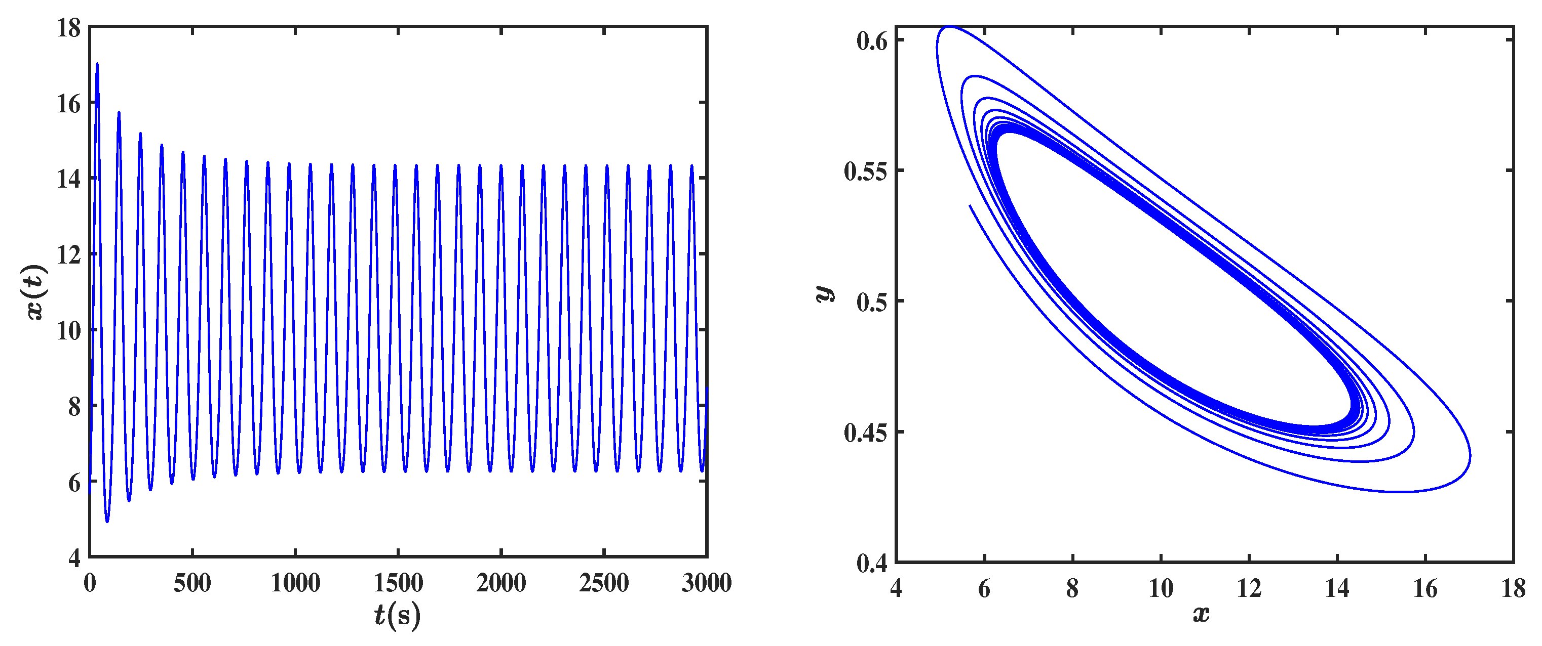
where the bounds $a_i,b_i,c_i(i=1,2)$ are explicitly computed cutoff values that delineate stable and unstable regions. The time evolution and phase portrait of the $(x,y)$ component are shown in Figure 1, with the parameters set $a=0.5$, $b=0.005$, $c=0.1$, $k=1$.

The presence of wide instability domains motivates extending the original integer-order model to a fractional-order framework. By replacing integer-order derivatives with fractional derivatives, one can effectively capture memory effects and nonlocal interactions inherent in real-world dislocation dynamics. The fractional-order generalization, introduced in the next section, will allow a broader range of dynamical behaviors, significantly enlarging the stability regions and more accurately reflecting experimental observations.

3. Fractional-Order Ananthakrishna Model

The fractional-order generalization of the Ananthakrishna model is defined as follows:

$$\left\{\begin{array}{cc}\hfill D^{{\alpha }_1}x(t)=& (1-a)x-b{x}^2-xy+y,\hfill \\ \hfill D^{{\alpha }_2}y(t)=& b(kb{x}^2-xy-y+az),\hfill \\ \hfill D^{{\alpha }_3}z(t)=& c(x-z),\hfill \end{array}\right.$$

(7)

where $D^{{\alpha }_i}(0<{\alpha }_i<1,i=1,2,3)$ are Caputo derivatives, defined by [37,38]:

$$D^{{\alpha }_i}u(t)={\displaystyle \frac{1}{\Gamma (1-{\alpha }_i)}}{\int }_0^t{\displaystyle \frac{{\partial }_{s}u(s)}{{(t-s)}^{{\alpha }_i}}}ds,0<{\alpha }_i<1.$$

(8)

The initial values are taken in accordance with the corresponding integer-order model.

To analyze the stability of model (7), we use the following fractional-order stability criterion, which has been widely adopted in the analysis of fractional-order dynamical models [39].

Theorem 1

([40]). Consider the incommensurate fractional-order model

$$D^{\alpha }x(t)=f(x(t)),x(0)=x_0,$$

(9)

with fractional orders $\alpha =({\alpha }_1,{\alpha }_2,\dots ,{\alpha }_n),{\alpha }_i\in (0,1)$, and $x\in {\mathbb{R}}^n$. An equilibrium point of model (9), found by solving $f(x(t))=0$, is locally asymptotically stable if all eigenvalues λ of the Jacobian matrix ${\displaystyle J=\frac{\partial f}{\partial x}}$ at this point satisfy:

$$|arg(\lambda )|>{\displaystyle \frac{{\alpha }^{*}\pi }{2}},{\alpha }^{*}=max\{{\alpha }_1,{\alpha }_2,\dots ,{\alpha }_n\}.$$

We first illustrate the stability characteristics of the integer-order model by selecting parameters $k=1$, $a=0.4$, $b=0.01$, and $c=0.01$. Under these conditions, model (1) possesses three equilibrium points:

$$E_0(0,0,0),E_1(13.6603,0.5,13.6603),E_2(-3.6603,0.5,-3.6603).$$

Eigenvalue computations confirm that all three equilibria are unstable. Specifically, at $E_1$, the eigenvalues of the Jacobian are ${\lambda }_1=-0.3344$ and ${\lambda }_{2,3}=0.0023\pm 0.0375i$. The positive real parts of ${\lambda }_{2,3}$ render $E_1$ a saddle-focus equilibrium, thus unstable.

For the fractional-order model, Theorem 1 implies that $E_1$ is stable if

$$|arg({\lambda }_i)|=1.5095>{\displaystyle \frac{{\alpha }^{*}\pi }{2}},i=2,3,$$

leading to a stability condition ${\alpha }^{*}<0.9611$. Similarly, $E_2$ becomes stable when ${\alpha }^{*}<0.6226$. These observations highlight a critical distinction: while the classical model is entirely unstable, the fractional model demonstrates conditional stability under appropriate choices of ${\alpha }_i,i=1,2,3$.

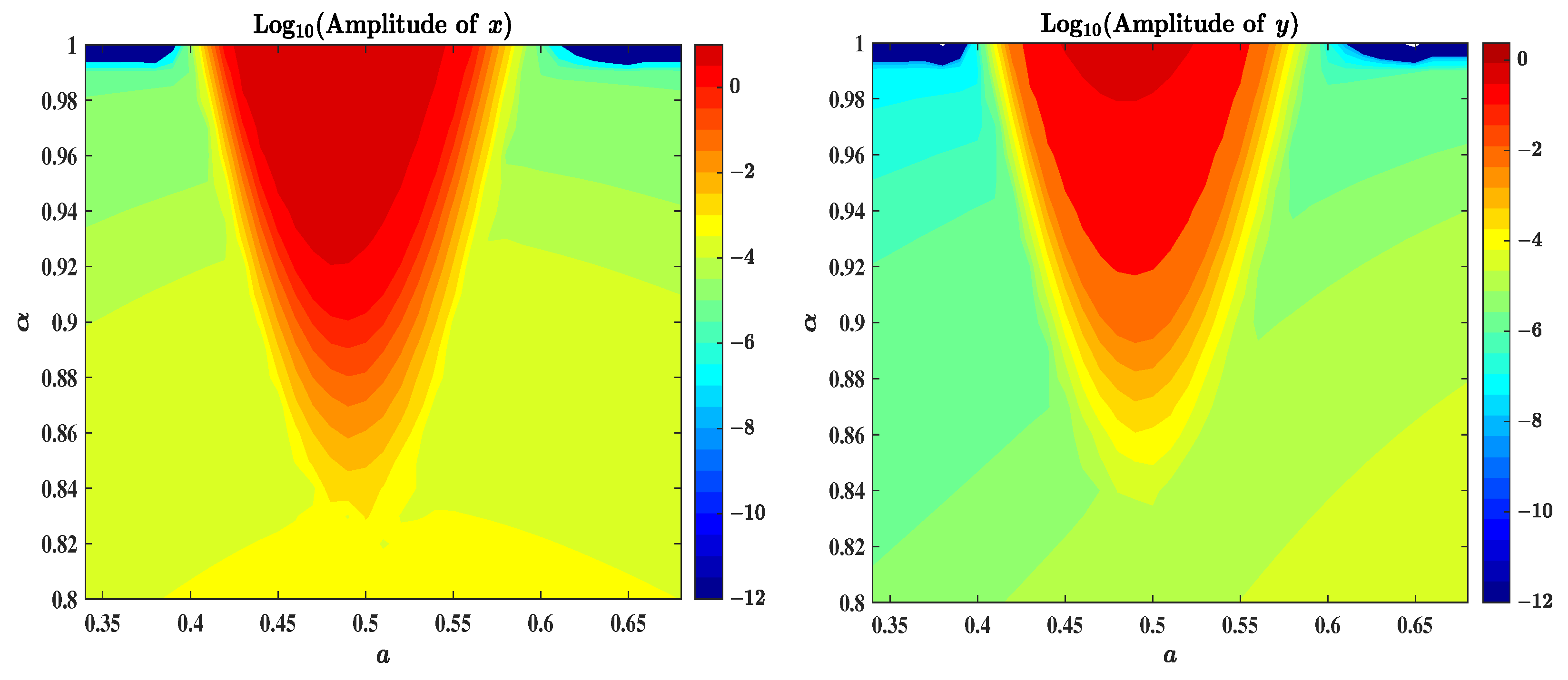
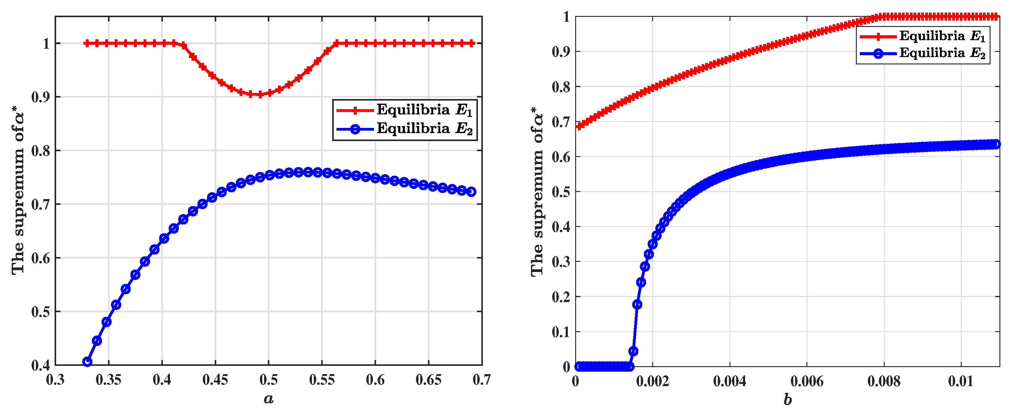
To further explore the effect of fractional-order derivatives on stability, we investigate how the supremum of fractional-order stability, ${\alpha }^{*}$, changes with respect to parameters a and b, respectively. Figure 2 shows the variation of the critical fractional-order threshold ${\alpha }^{*}$ for equilibria $E_1$ and $E_2$: the left panel demonstrates the dependence on parameter a within the range $(0.33,0.69)$ with fixed parameters $b=0.01$, $c=0.04$ and $k=1$, while the right panel shows the variation with respect to parameter b in the range $(0,0.011)$, with fixed parameters $a=0.04$, $c=0.04$ and $k=1$.

From these plots, we observe that equilibrium $E_2$ consistently displays smaller critical and wider margin ${\alpha }^{*}$ values compared to $E_1$, indicating greater sensitivity to fractional-order effects. Specifically, at equilibrium $E_2$, the supremum of ${\alpha }^{*}$ remains mostly below $0.8$ when varying a, and generally below $0.7$ when varying b. In contrast, equilibrium $E_1$ exhibits significantly higher robustness, with ${\alpha }^{*}$ values consistently above $0.9$ across both parameter variations. For example, at the representative point $a=0.5$ (left panel), the stability threshold at equilibrium $E_1(7.0711,0.5,7.0711)$ is ${\alpha }^{*}=0.9068$, signifying stability for fractional orders below this critical value. Similarly, the right panel clearly illustrates that equilibrium $E_1$ maintains large critical ${\alpha }^{*}$ values even as b approaches the upper limit of its investigated range, highlighting the general capability of the fractional-order model to substantially extend stability regions compared to its integer-order counterpart.

4. Fast Finite Difference Approximation for Fractional Ananthakrishna Model

In this section, we propose a computationally efficient numerical scheme for the fractional Ananthakrishna model (7), based on an accelerated approximation of the Caputo fractional derivative. The primary idea leverages a fast L1 operator which, although widely applied, is briefly described below for completeness and clarity.

Consider a uniform partition of the interval $[0,T]$ into N subintervals with time step size $h=T/N$, and define $t_n=nh$, $n=0,1,\dots ,N$. To approximate the Caputo derivative $D^{\alpha }u$, the classical L1 scheme employs piecewise linear interpolation over each subinterval:

$${\Pi }_{1,j}u(t)=u(t_j){\displaystyle \frac{t_{j+1}-t}{h}}+u(t_{j+1}){\displaystyle \frac{t-t_j}{h}},j=0,1,\cdots ,N-1.$$

The corresponding L1 approximation of $D^{\alpha }u(t_n)$ is given by [20]:

$$\begin{array}{cc}\hfill D^{\alpha }u(t_n)\approx & {\displaystyle \frac{1}{\Gamma (1-\alpha )}}\sum _{j=0}^{n-1}{\int }_{t_j}^{t_{j+1}}{\displaystyle \frac{{\partial }_s{\Pi }_{1,j}u(s)}{{(t_n-s)}^{\alpha }}}ds\hfill \\ \hfill =& {\displaystyle \frac{1}{\Gamma (2-\alpha )h^{\alpha }}}\left[a_0^{\alpha }u(t_n)-\sum _{i=1}^{n-1}(a_{n-1-i}^{\alpha }-a_{n-i}^{\alpha })u(t_i)-a_{n-1}^{\alpha }u(t_0)\right],\hfill \end{array}$$

(10)

with coefficients $a_i^{\alpha }={(i+1)}^{1-\alpha }-i^{1-\alpha }$. This scheme captures the non-local memory effect of fractional derivatives, as the computation at $t_n$ depends on all previous steps. However, direct implementation has computational complexity $\mathcal{O}(N^2)$ and storage complexity $\mathcal{O}(N)$, which are prohibitive for large N.

To enhance computational efficiency, we adopt the accelerated L1 approach, decomposing $D^{\alpha }u(t_n)$ into local and history components:

$$D^{\alpha }u(t_n)=D_l^{\alpha }(t_n)+D_h^{\alpha }(t_n),$$

where

$$D_l^{\alpha }(t_n)={\displaystyle \frac{1}{\Gamma (1-\alpha )}}{\int }_{t_{n-1}}^{t_n}{\displaystyle \frac{{\partial }_{s}u(s)}{{(t_n-s)}^{\alpha }}}ds,D_h^{\alpha }(t_n)={\displaystyle \frac{1}{\Gamma (1-\alpha )}}{\int }_0^{t_{n-1}}{\displaystyle \frac{{\partial }_{s}u(s)}{{(t_n-s)}^{\alpha }}}ds.$$

(11)

The local $D_l^{\alpha }(t_n)$ is approximated as:

$${\displaystyle D_l^{\alpha }(t_n)\approx \frac{1}{\Gamma (1-\alpha )}{\int }_{t_{n-1}}^{t_n}\frac{{\Pi }_{1,n-1}{u}^{\prime }(s)}{{(t_n-s)}^{\alpha }}ds=\frac{u(t_n)-u(t_{n-1})}{\Gamma (2-\alpha )h^{\alpha }}.}$$

(12)

For the history term $D_h^{\alpha }(t_n)$, integration by parts gives

$${\displaystyle D_h^{\alpha }(t_n)=\frac{1}{\Gamma (1-\alpha )}\left[\frac{u(t_{n-1})}{h^{\alpha }}-\frac{u(t_0)}{t_n^{\alpha }}-\alpha {\int }_0^{t_{n-1}}\frac{u(s)ds}{{(t_n-s)}^{1+\alpha }}\right].}$$

(13)

The kernel function ${(t_n-s)}^{-\alpha -1}$ is efficiently approximated by a sum-of-exponentials (SOE) with any prescribed error tolerance $\epsilon \ll 1$ [31]:

$${\displaystyle |\frac{1}{t^{1+\alpha }}-\sum _{i=1}^{N_{\epsilon }^{\alpha }}{\omega }_i^{\alpha }{e}^{-s_i^{\alpha }t}|\le \epsilon ,\forall t\in [h,T],}$$

where the number of terms $N_{\epsilon }^{\alpha }$ is significantly smaller than N. This decomposition replaces the direct evaluation of convolution history with a sum of $N_{\epsilon }^{\alpha }$ exponentials that can be computed recursively, significantly reducing both memory usage and CPU time. Incorporating this approximation, we obtain

$${\displaystyle D_h^{\alpha }(t_n)\approx \frac{1}{\Gamma (1-\alpha )}\left[\frac{u(t_{n-1})}{h^{\alpha }}-\frac{u(t_0)}{t_n^{\alpha }}-\alpha \sum _{i=1}^{N_{\epsilon }^{\alpha }}{\omega }_i^{\alpha }{U}_{h,i}^{\alpha }(t_n)\right],}$$

(14)

with the history integral approximated recursively as

$$\begin{array}{cc}\hfill U_{h,i}^{\alpha }(t_n)=& {\displaystyle {\int }_0^{t_{n-1}}{e}^{-s_i^{\alpha }(t_n-s)}u(s)ds}\hfill \\ \hfill =& e^{-s_i^{\alpha }h}{U}_{h,i}^{\alpha }(t_{n-1})+{\int }_{t_{n-2}}^{t_{n-1}}{e}^{-s_i^{\alpha }(t_n-s)}u(s)ds\hfill \\ \hfill \approx & e^{-s_i^{\alpha }h}{U}_{h,i}^{\alpha }(t_{n-1})+{\int }_{t_{n-2}}^{t_{n-1}}{e}^{-s_i^{\alpha }(t_n-s)}{\Pi }_{1,n-2}u(s)ds\hfill \\ \hfill =& e^{-s_i^{\alpha }h}{U}_{h,i}^{\alpha }(t_{n-1})+{\tilde{a}}_i^{\alpha }u(t_{n-1})+{\tilde{b}}_i^{\alpha }u(t_{n-2}),\hfill \end{array}$$

(15)

where the positive coefficients ${\tilde{a}}_i^{\alpha },{\tilde{b}}_i^{\alpha }$ are explicitly given by integrals over exponential kernels:

$$\begin{array}{cc}\hfill {\tilde{a}}_i^{\alpha }=& {\int }_{t_{n-2}}^{t_{n-1}}{e}^{-s_i^{\alpha }(t_n-s)}{\displaystyle \frac{s-t_{n-2}}{h}}ds={\displaystyle \frac{e^{-s_i^{\alpha }h}}{{(s_i^{\alpha })}^{2}h}}(e^{-s_i^{\alpha }h}-1+s_i^{\alpha }h),\hfill \\ \hfill {\tilde{b}}_i^{\alpha }=& {\int }_{t_{n-2}}^{t_{n-1}}{e}^{-s_i^{\alpha }(t_n-s)}{\displaystyle \frac{s-t_{n-1}}{-h}}ds={\displaystyle \frac{e^{-s_i^{\alpha }h}}{{(s_i^{\alpha })}^{2}h}}(1-e^{-s_i^{\alpha }h}-e^{-s_i^{\alpha }h}{s}_i^{\alpha }h).\hfill \end{array}$$

(16)

Thus, we define the fast fractional operator $F_t^{\alpha }$ as:

$$F_t^{\alpha }{u}_n={\displaystyle \frac{u_n-u_{n-1}}{\Gamma (2-\alpha )h^{\alpha }}}+{\displaystyle \frac{1}{\Gamma (1-\alpha )}}\left[{\displaystyle \frac{u_{n-1}}{h^{\alpha }}}-{\displaystyle \frac{u_0}{t_n^{\alpha }}}-\alpha \sum _{i=1}^{N_{\epsilon }^{\alpha }}{\omega }_i^{\alpha }{U}_{h,i}^{n,\alpha }\right],n=1,2,\dots ,N,$$

(17)

where $U_{h,i}^{1,\alpha }=0$, and for $2\le n\le N-1$,

$$U_{h,i}^{n,\alpha }=e^{-s_i^{\alpha }h}{U}_{h,i}^{n-1,\alpha }+{\tilde{a}}_i^{\alpha }{u}_{n-1}+{\tilde{b}}_i^{\alpha }{u}_{n-2},i=1,\cdots ,N_{\epsilon }^{\alpha }.$$

(18)

As shown in [31], the truncation error of the fast finite difference operator $F_t^{\alpha }$ is of order $(h^{2-\alpha }+\epsilon )$, provided that $u\in C^2[0,T]$. Compared to the direct L1 scheme, while maintaining the same level of convergence accuracy, this fast scheme reduces the storage cost from $\mathcal{O}(N)$ to $\mathcal{O}(N_{\epsilon }^{\alpha })$ and computational cost from $\mathcal{O}(N^2)$ to $\mathcal{O}(N{N}_{\epsilon }^{\alpha })$.

Now applying this accelerated L1 discretization to the fractional Ananthakrishna model (7), we derive the semi-implicit numerical scheme:

$$\left\{\begin{array}{cc}\hfill F_t^{{\alpha }_1}{x}_n=& (1-a)x_{n-1}-b{x}_{n-1}{x}_n-x_{n-1}{y}_n+y_{n-1},\hfill \\ \hfill F_t^{{\alpha }_2}{y}_n=& b(kb{x}_{n-1}{x}_n-x_{n-1}{y}_n-y_n+a{z}_{n-1}),\hfill \\ \hfill F_t^{{\alpha }_3}{z}_n=& c(x_n-z_n).\hfill \end{array}\right.$$

(19)

This implicit discretization can be rearranged and computed efficiently in a decoupled manner. In fact, the expression of $F_t^{\alpha }$ defined in (17) can be rewritten as

$$F_t^{\alpha }{u}_n={\displaystyle \frac{1}{\Gamma (2-\alpha )h^{\alpha }}}\left[u_n-\left(\alpha u_{n-1}+{\displaystyle \frac{1-\alpha }{n^{\alpha }}}{u}_0+\alpha (1-\alpha )h^{\alpha }\sum _{i=1}^{N_{\epsilon }^{\alpha }}{\omega }_i^{\alpha }{U}_{h,i}^{n,\alpha }\right)\right]:={\displaystyle \frac{1}{d_{\alpha }}}(u_n-H_{\alpha }),$$

(20)

where the coefficient $d_{\alpha }=\Gamma (2-\alpha )h^{\alpha }$, $H_{\alpha }$ represents the history terms. Then the discrete problem (19) can be equivalently expressed by

$$\left\{\begin{array}{cc}\hfill x_n=& {\displaystyle \frac{H_{{\alpha }_1}+d_{{\alpha }_1}[(1-a)x_{n-1}-x_{n-1}{y}_n+y_{n-1}]}{1+b{d}_{{\alpha }_1}{x}_{n-1}}},\hfill \\ \hfill y_n=& {\displaystyle \frac{H_{{\alpha }_2}+b{d}_{{\alpha }_2}(kb{x}_{n-1}{x}_n+a{z}_{n-1})}{1+b{d}_{{\alpha }_2}(x_{n-1}+1)}},\hfill \\ \hfill z_n=& {\displaystyle \frac{H_{{\alpha }_3}+c{d}_{{\alpha }_3}{x}_n}{1+c{d}_{{\alpha }_3}}}.\hfill \end{array}\right.$$

(21)

Substituting the second equation into the right side of the first one, the discrete problem can be decouplly computed as follows:

$$\left\{\begin{array}{cc}\hfill x_n=& {\displaystyle \frac{[1+b{d}_{{\alpha }_2}(x_{n-1}+1)]\{H_{{\alpha }_1}+d_{{\alpha }_1}[(1-a)x_{n-1}+y_{n-1}]\}-d_{{\alpha }_1}{x}_{n-1}(H_{{\alpha }_2}+ab{d}_{{\alpha }_2}{z}_{n-1})}{(1+b{d}_{{\alpha }_1}{x}_{n-1})[1+b{d}_{{\alpha }_2}(x_{n-1}+1)]+k{b}^2{d}_{{\alpha }_1}{d}_{{\alpha }_2}{(x_{n-1})}^2}},\hfill \\ \hfill y_n=& {\displaystyle \frac{H_{{\alpha }_2}+b{d}_{{\alpha }_2}(kb{x}_{n-1}{x}_n+a{z}_{n-1})}{1+b{d}_{{\alpha }_2}(x_{n-1}+1)}},\hfill \\ \hfill z_n=& {\displaystyle \frac{H_{{\alpha }_3}+c{d}_{{\alpha }_3}{x}_n}{1+c{d}_{{\alpha }_3}}}.\hfill \end{array}\right.$$

(22)

The following lemma guarantees the positivity of the numerical solutions.

Lemma 1.

Assume that the initial values $x_0,y_0,z_0$ of the fractional Ananthakrishna model (7) are positive and the time step size h is sufficiently small. Suppose further that $0<a<1$. Then, for all $1\le n\le N$, the numerical solutions $x(n),y(n),z(n)$ generated by the scheme (19) remain positive.

Proof. 

We proceed by mathematical induction. Assume that $x(j)>0$, $y(j)>0$ and $z(j)>0$ for all $0\le j\le n-1$.

We first show that $y_n>0$. By substituting the expression for $x_n$ from the first equation of (21) into the second equation, we obtain

$$y_n={\displaystyle \frac{H_{{\alpha }_2}+ab{d}_{{\alpha }_2}{z}_{n-1}+k{b}^2{d}_{{\alpha }_2}{x}_{n-1}\frac{H_{{\alpha }_1}+d_{{\alpha }_1}[(1-a)x_{n-1}+y_{n-1}]}{1+b{d}_{{\alpha }_1}{x}_{n-1}}}{1+b{d}_{{\alpha }_2}(x_{n-1}+1)+\frac{k{b}^2{d}_{{\alpha }_1}{d}_{{\alpha }_2}{(x_{n-1})}^2}{1+b{d}_{{\alpha }_1}{x}_{n-1}}}}.$$

(23)

From the positivity of the coefficients ${\tilde{a}}_i^{\alpha },{\tilde{b}}_i^{\alpha }>0$ in (16) and the recurrence relation for the history term $U_{h,i}^{n,\alpha }$ in (18), it follows that all $U_{h,i}^{n,\alpha }>0$ for $i=1,\dots ,N_{\epsilon }^{\alpha }$. Consequently, the history terms $H_{{\alpha }_1},H_{{\alpha }_2}>0$ defined in (20) are strictly positive. Since all quantities in the numerator and denominator of the above expression for $y_n$ are positive, we conclude that $y_n>0$.

Next, we consider the positivity of $x_n>0$. From the definition of $H_{{\alpha }_1}$, we have $H_{{\alpha }_1}>{\alpha }_1{x}_{n-1}$. Substituting this into the expression for $x_n$ in (21), the numerator satisfies the bound:

$$H_{{\alpha }_1}+d_{{\alpha }_1}[(1-a)x_{n-1}-x_{n-1}{y}_n+y_{n-1}]\ge x_{n-1}[{\alpha }_1+d_{{\alpha }_1}(1-a-y_n)].$$

If $y_n<1-a$, then the bracketed term is positive, and thus $x_n>0$. If instead $y_n\ge 1-a$, define ${\displaystyle M_y=\underset{1\le n\le N}{max}{y}_n}$. Then the positivity of $x_n$ is ensured provided that the time step size h satisfies the constraint

$$h^{{\alpha }_1}<{\displaystyle \frac{{\alpha }_1}{\Gamma (2-{\alpha }_1)(M_y+a-1)}}.$$

(24)

Finally, the positivity of $z_n$ follows immediately from the third equation in (21), as it is computed from positive values of $x_n$. □

Remark 1.

The constraint on the time step size h imposed in (24) is mild. Indeed, the denominator of the inequality contains the term $M_y$, the maximum value of the numerical solution $y_n$. As will be demonstrated rigorously in the subsequent stability analysis, the numerical solution $y_n$ remain bounded above, with a bound dependent explicitly on initial conditions, model parameters, and fractional orders of derivatives. Furthermore, numerical experiments in the following section consistently show that $y_n$ rapidly converges to its equilibrium value (approximately $0.5$) after initial transient oscillations, rarely exceeding the value 1. Consequently, the upper bound condition for h is easily satisfied in practice, making this restriction effectively negligible for typical numerical simulations. Notably, as ${\alpha }_1\to 1$, the constraint on h given in (24) remains mild, since it converges to a finite positive constant ${\displaystyle \frac{1}{M_y+a-1}}$, thereby avoiding any sharp deterioration in the allowed time step.

The following property is useful in the stability analysis.

Lemma 2

([31]). For any mesh function $u=\left\{u_k\right|0\le k\le N\}$ defined on ${\left\{t_k\right\}}_{k=0}^N$, the following inequality holds: for $1\le n\le N$,

$$h\sum _{k=1}^n(F_t^{\alpha }{u}_k)u_k\ge {\displaystyle \frac{t_n^{-\alpha }-2\alpha \epsilon t_{n-1}}{2\Gamma (1-\alpha )}}h\sum _{k=1}^n{(u_k)}^2-{\displaystyle \frac{t_n^{1-\alpha }-\alpha (1-\alpha )\epsilon t_{n-1}h}{2\Gamma (2-\alpha )}}{(u_0)}^2.$$

(25)

The stability of the proposed numerical scheme is established by the following theorem.

Theorem 2.

Suppose that the parameters satisfy $0<a<1,b>0$, and $c>a$, and let the SOE approximation error ε be sufficiently small. Then the numerical solution of the discrete model (19) is stable and satisfies the following estimate for any $1\le n\le N$:

$$\begin{array}{cc}\hfill & h\sum _{k=1}^n\left[k{b}^2{(x_k)}^2+2{(y_k)}^2+{(z_k)}^2\right]\hfill \\ \hfill \le & {\displaystyle \frac{1}{\mu }}exp\left({\displaystyle \frac{1}{\mu }}max\left\{{\displaystyle \frac{{(1-a)}^2}{\mu }}(2+{\displaystyle \frac{c}{2k{b}^2\mu }}),{\displaystyle \frac{1}{\mu }}(k{b}^2+{\displaystyle \frac{c}{4\mu }}),{\displaystyle \frac{a^{2}b}{2}}\right\}\right)\left\{\right[\rho ({\displaystyle \frac{c}{2\mu }}+2k{b}^2)+\hfill \\ \hfill & {\displaystyle \frac{{(1-a)}^{2}h}{\mu }}(2k{b}^2+{\displaystyle \frac{c}{2\mu }})]{(x_0)}^2+\left[2\rho +{\displaystyle \frac{h}{\mu }}(2k{b}^2+{\displaystyle \frac{c}{2\mu }})\right]{(y_0)}^2+(\rho +{\displaystyle \frac{a^{2}bh}{2}}){(z_0)}^2\},\hfill \end{array}$$

(26)

where ${\displaystyle \rho =\underset{i=1,2,3}{max}\frac{T^{1-{\alpha }_i}}{2\Gamma (2-{\alpha }_i)}}$, ${\displaystyle \mu =\underset{i=1,2,3}{min}\frac{T^{-{\alpha }_i}-2{\alpha }_i\epsilon T}{2\Gamma (1-{\alpha }_i)}}$.

Proof. 

Multiplying the first two equations of (19) by $k{b}^{2}h{x}_j$ and $h{y}_j$, respectively, and summing from $j=1$ to n, we obtain

$$\begin{array}{cc}\hfill k{b}^{2}h\sum _{j=1}^n(F_t^{{\alpha }_1}{x}_j)x_j=& k{b}^{2}h\sum _{j=1}^n[(1-a)x_{j-1}-b{x}_{j-1}{x}_j-x_{j-1}{y}_j+y_{j-1}]x_j,\hfill \\ \hfill h\sum _{j=1}^n(F_t^{{\alpha }_2}{y}_j)y_j=& hb\sum _{j=1}^n(kb{x}_{j-1}{x}_j-x_{j-1}{y}_j-y_j+a{z}_{j-1})y_j.\hfill \end{array}$$

(27)

Adding these two equalities, discarding nonnegative terms, and employing Lemma 1 and Young’s inequality yield

$$\begin{array}{cc}\hfill & k{b}^{2}h\sum _{j=1}^n(F_t^{{\alpha }_1}{x}_j)x_j+h\sum _{j=1}^n(F_t^{{\alpha }_2}{y}_j)y_j+bh\sum _{j=1}^n{y}_j^2\hfill \\ \hfill =& (1-a)k{b}^{2}h\sum _{j=1}^n{x}_{j-1}{x}_j+k{b}^{2}h\sum _{j=1}^n{y}_{j-1}{x}_j+abh\sum _{j=1}^n{z}_{j-1}{y}_j\hfill \\ \hfill \le & {\displaystyle \frac{k{(1-a)}^2{b}^2}{{\mu }_1^n}}h\sum _{j=1}^n{x}_{j-1}^2+{\displaystyle \frac{k{b}^2}{{\mu }_1^n}}h\sum _{j=1}^n{y}_{j-1}^2+{\displaystyle \frac{k{b}^2}{2}}{\mu }_1^{n}h\sum _{j=1}^n{x}_j^2+{\displaystyle \frac{a^{2}b}{4}}h\sum _{j=1}^n{z}_{j-1}^2+bh\sum _{j=1}^n{y}_j^2.\hfill \end{array}$$

Utilizing Lemma 2, the above estimate simplifies to

$$\begin{array}{cc}\hfill & {\displaystyle \frac{k{b}^2}{2}}{\mu }_1^{n}h\sum _{j=1}^n{x}_j^2+{\mu }_2^{n}h\sum _{j=1}^n{y}_j^2\hfill \\ \hfill \le & {\displaystyle \frac{k{(1-a)}^2{b}^2}{{\mu }_1^n}}h\sum _{j=1}^n{x}_{j-1}^2+{\displaystyle \frac{k{b}^2}{{\mu }_1^n}}h\sum _{j=1}^n{y}_{j-1}^2+{\displaystyle \frac{a^{2}b}{4}}h\sum _{j=1}^n{z}_{j-1}^2+k{b}^2{\rho }_1^n{x}_0^2+{\rho }_2^n{y}_0^2.\hfill \end{array}$$

(28)

Next, multiplying the third equation in (19) by $h{z}_j$, summing over $j=1,\cdots ,n$, and using similar arguments yield

$${\mu }_3^{n}h\sum _{j=1}^n{z}_j^2\le {\displaystyle \frac{hc}{4}}\sum _{j=1}^n{x}_j^2+{\rho }_3^n{z}_0^2.$$

Furthermore, multiplying the first equation by $h{x}_j$, summing similarly, gives the following bound:

$${\mu }_1^{n}h\sum _{j=1}^n{x}_j^2\le {\displaystyle \frac{2{(1-a)}^2}{{\mu }_1^n}}h\sum _{j=1}^n{x}_{j-1}^2+{\displaystyle \frac{2h}{{\mu }_1^n}}\sum _{j=1}^n{y}_{j-1}^2+2{\rho }_1^n{x}_0^2.$$

Substituting this into the previous inequality for $z_n$, we have

$${\mu }_3^{n}h\sum _{j=1}^n{z}_j^2\le {\displaystyle \frac{ch}{2{({\mu }_1^n)}^2}}\left[{(1-a)}^2\sum _{j=1}^n{x}_{j-1}^2+\sum _{j=1}^n{y}_{j-1}^2\right]+{\displaystyle \frac{c{\rho }_1^n}{2{\mu }_1^n}}{x}_0^2+{\rho }_3^n{z}_0^2.$$

(29)

Combing (28) with (29) and noting that ${\mu }_i^n\ge \mu$ and ${\rho }_i^n\le \rho$ for $i=1,2,3$, we derive

$$\begin{array}{cc}\hfill & \mu h\sum _{j=1}^n\left(k{b}^2{x}_j^2+2y_j^2+z_j^2\right)\hfill \\ \hfill \le & max\left\{{\displaystyle \frac{{(1-a)}^2}{\mu }}(2+{\displaystyle \frac{c}{2k{b}^2\mu }}),{\displaystyle \frac{1}{\mu }}(k{b}^2+{\displaystyle \frac{c}{4\mu }}),{\displaystyle \frac{a^{2}b}{2}}\right\}h\sum _{j=1}^{n-1}\left(k{b}^2{x}_j^2+2y_j^2+z_j^2\right)\hfill \\ \hfill +& \left[\rho ({\displaystyle \frac{c}{2\mu }}+2k{b}^2)+{\displaystyle \frac{{(1-a)}^{2}h}{\mu }}(2k{b}^2+{\displaystyle \frac{c}{2\mu }})\right]x_0^2+\left[2\rho +{\displaystyle \frac{h}{\mu }}(2k{b}^2+{\displaystyle \frac{c}{2\mu }})\right]y_0^2+(\rho +{\displaystyle \frac{a^{2}bh}{2}})z_0^2.\hfill \end{array}$$

(30)

Applying the discrete Gronwall lemma, we obtain the desired stability estimate (26). The proof is completed. □

5. Numerical Experiments

In this section, we present numerical examples to demonstrate the complex dynamical behaviors of the fractional-order Ananthakrishna model (7) using the proposed discretization scheme (22). The numerical experiments contain three parts: the largest Lyapunov exponent test, bifurcation diagrams, and numerical phase diagrams combined with a computational efficiency comparison. Here, $\epsilon$ denotes the tolerated error in approximating the fractional kernel by SOE. To avoid bias in the bifurcation and phase simulations, we set $\epsilon ={10}^{-9}$. For the Lyapunov exponent calculations—where sensitivity to perturbations is higher—we use a tighter tolerance of $\epsilon ={10}^{-12}$. All numerical experiments are conducted on a computer with an 11th Gen Intel(R) Core(TM) i7-1165G7 CPU @ 2.80 GHz, 32 GB RAM, and Windows 11 operating system. No parallelization or multi-core acceleration is employed.

5.1. Largest Lyapunov Exponent Analysis

The largest Lyapunov exponent provides an essential measure for stability and chaos detection in dynamical systems [41]. We first use it to verify the stability thresholds derived theoretically in Section 3. The computation uses the full simulation interval without discarding any transient phase.

Considering the commensurate fractional-order case (${\alpha }_1={\alpha }_2={\alpha }_3=\alpha$), we fix parameters as $a=0.4$, $b=0.01$, $c=0.01$, $k=1$, and initial values $(x_0,y_0,z_0)=(13.66,0.5,13.66)$, with the step size $h=0.1$ and SOE accuracy $\epsilon ={10}^{-12}$. The largest Lyapunov exponent as a function of fractional order $\alpha$ is presented in Figure 3(left). It can be observed that the Lyapunov exponent remains negative when $\alpha \le 0.96$ and becomes positive thereafter, consistent with the theoretical stability boundary ${\alpha }^{*}=0.9611$ found in Section 3. Figure 3(right) further confirms this by illustrating the temporal evolution of the largest Lyapunov exponent at fractional orders $\alpha =0.94$ and $\alpha =0.98$.

Subsequently, we investigate the dependence of the largest Lyapunov exponent on parameters $\alpha$ and a, with fixed $b=0.01$, $c=0.04$, and $k=1$. Figure 4(left) reveals a non-monotonic dependence of stability on a, showcasing an unstable region at intermediate a values. This unstable region aligns closely with the interval in which the critical stability threshold ${\alpha }^{*}$ significantly decreases, as depicted by the concave portion of the curve in Figure 2(left). Figure 4(right) reinforces this observation by showing clear distinctions in Lyapunov exponent trajectories at $\alpha =0.89$ (stable) and $0.91$ (unstable), confirming the critical stability threshold around ${\alpha }^{*}=0.9068$ when $a=0.5$.

5.2. Bifurcation Analysis

We now investigate the bifurcation behavior of the fractional-order Ananthakrishna model. Figure 5 presents two-dimensional bifurcation diagrams of state variables x and y under variations of the fractional order $\alpha$ and parameter a, with $b=0.01$, $c=0.04$, and $h=0.1$, $\epsilon ={10}^{-9}$. The left panel illustrates that for $a=0.5$, the solution remains stable when $\alpha \le 0.9$. However, as $\alpha$ increases beyond the critical threshold ${\alpha }^{*}=0.9068$, the solution becomes unstable, which aligns with the analysis based on the largest Lyapunov exponent. The right panel shows that at $\alpha =0.95$, varying the parameter a leads the system to undergo a transition from a steady state to an unstable regime (including $a=0.5$), and then back to stability.

Moreover, Figure 6 presents three-dimensional bifurcation diagrams for x and y. It is observed that as $\alpha$ decreases, the critical bifurcation thresholds in the $(a,\alpha )$ plane shift to the right, meaning that larger values of a are required to destabilize the system. This trend confirms that fractional-order derivatives effectively delay the loss of stability and expand the parameter regime where stable equilibrium persists. Such observations are fully consistent with the stability and Lyapunov analyses discussed earlier.

To provide a more quantitative counterpart to the 3D bifurcation diagrams, Figure 7 displays two-dimensional colored maps of the logarithmic maximum amplitudes of $x(t)$ and $y(t)$. Given the wide range of amplitude values (approximately ${10}^{-12}$ to 14 for x, and ${10}^{-13}$ to $0.38$ for y), a logarithmic color scale is employed to ensure sufficient contrast across the parameter space. These heatmaps clearly reveal the transition from stable to unstable dynamics across the $(a,\alpha )$ plane and allow more precise identification of oscillatory intensity.

For all bifurcation-related plots (Figure 5, Figure 6 and Figure 7), the total simulation time is set to $T=2000$, and the initial transient phase is discarded; only the trajectory from $t=1800$ to $t=2000$ is used to generate the plots.

5.3. Phase and Time Diagram Analysis with Efficiency Comparison

We further validate the stability properties by examining the evolution numerical solutions for varying fractional orders. Setting parameters $a=0.4$, $b=0.01$, $c=0.01$, $k=1$, and initial conditions $(x_0,y_0,z_0)=(13,0.5,13)$, $h=0.1$, the numerical solutions of the fractional model for (i) incommensurate order ${\alpha }_1=0.7,{\alpha }_2=0.8,{\alpha }_3=0.9$, (ii) commensurate order ${\alpha }_1={\alpha }_2={\alpha }_3=0.95$, (iii) ${\alpha }_1={\alpha }_2={\alpha }_3=0.97$, along with the integer-order model (discretized by the Runge-Kutta scheme), are displayed in Figure 8 and Figure 9. It’s observed that the solutions remain stable for fractional orders below the threshold (${\alpha }^{*}=0.9611$), while exhibiting periodic and unstable behaviors above this critical value, consistent with theoretical predictions.

Figure 8 also indicates that as the fractional derivative order approaches the critical value, it takes longer to achieve stability. In support of this, the estimated damping rate is approximately $0.0116$ for the case ${\alpha }_1=0.7$, ${\alpha }_2=0.8$, ${\alpha }_3=0.9$, while it drops to about $2.4057\times {10}^{-4}$ when ${\alpha }_1={\alpha }_2={\alpha }_3=0.95$, clearly reflecting the slower convergence near the critical threshold.

To further illustrate this delay, we present two additional time-series plots in Figure 10, comparing the evolution of $x(t)$ for the integer-order and fractional-order models. It is observed that the integer-order system reaches a periodic regime around $t=620$, while the fractional-order system takes significantly longer, stabilizing around $t=3099$. This comparison highlights the prolonged transient behavior induced by memory effects in fractional dynamics. Additionally, the phase portraits in Figure 9 reveal that the fractional-order model exhibits smoother and more regular trajectories compared to the integer-order case, highlighting the damping and memory effects inherent in fractional derivatives.

Finally, to demonstrate the computational advantages of the fast L1 scheme, we compare it against the classical L1 and Grünwald-Letnikov (GL) schemes. The GL scheme is a first-order approximation for the Caputo derivative and takes the form [38]:

$$D^{\alpha }u(t_n)\approx \sum _{j=0}^n{c}_j^{\alpha }u(t_{n-j}),0<\alpha <1,$$

where $c_0^{\alpha }=h^{-\alpha }$, $c_j^{\alpha }=(1-{\displaystyle \frac{1+\alpha }{j}})c_{j-1}^{\alpha }$, $j=1,\dots ,N$. Figure 11 shows that the three methods yield nearly identical numerical results.

Table 1. Number of SOE terms $N_{\epsilon }^{\alpha }$ in the fast L1 scheme for different time step sizes h, with $\alpha =0.9$, $T=2000$, and $\epsilon ={10}^{-9}$.

h	0.08	0.05	0.02	0.01	0.008	0.005	0.004
$N_T$	25,000	40,000	100,000	200,000	250,000	400,000	500,000
$N_{\epsilon }^{\alpha }$	62	64	67	69	70	72	73

displays the number of SOE terms $N_{\epsilon }^{\alpha }$ under different step sizes h, with a fixed final time $T=2000$, fractional order $\alpha =0.9$, and error tolerance $\epsilon ={10}^{-9}$. As shown, $N_{\epsilon }^{\alpha }$ increases only slightly from 62 to 73 as the time step size h decreases from $0.08$ to $0.004$ (corresponding to $N_T$ increasing from $25,000$ to $500,000$), in contrast to the classical L1 scheme, which requires storing all past values.

Moreover, as illustrated in the left panel of Figure 12, the CPU time of the fast L1 scheme grows linearly with $\mathrm{Log}(N)$, while the CPU time for both L1 and GL schemes increases quadratically.

Table 2. CPU Time for different number of total steps.

	h	0.08	0.05	0.02	0.01	0.008	0.005	0.004
cpu Time
Fast L1		0.3105	0.3667	0.77	1.4329	1.7915	2.8346	3.5205
L1		3.6326	9.4935	58.5078	452.8233	710.565	1910.0481	2879.9324
GL		4.3556	11.057	59.4566	397.1266	687.96	1894.3818	2981.8201

presents the detailed CPU timings corresponding to these tests. These results clearly demonstrate the superior computational efficiency of the fast L1 method. The influence of the prescribed error $\epsilon$ on the SOE number $N_{\epsilon }^{\alpha }$ and CPU time is investigated in the right panel of Figure 12. As expected, $N_{\epsilon }^{\alpha }$ increases linearly with $log\epsilon$; however, the CPU time remains nearly constant. This indicates that the cost of computing the SOE history terms is negligible compared to the total cost, especially for large $N_T$. Therefore, a small $\epsilon$ can be selected to ensure high accuracy without compromising computational efficiency.

To further evaluate the trade-off between accuracy and efficiency, we compare the performance of the classical L1 scheme and the fast L1 scheme through error–CPU time diagrams, as shown in Figure 13. In this test, we simulate the system up to final time $T=500$ using various time step sizes $h=0.25,0.1,0.05,0.025,0.0125,0.01$. For each h, we compute the numerical solution and measure its absolute error at $T=500$. The reference solution is obtained using the fast L1 scheme with a very small step size $h={10}^{-4}$ and a tight SOE tolerance $\epsilon ={10}^{-12}$. The reference values at $T=500$ are $x_{ref}=13.763122$, $y_{ref}=0.497306$, $z_{ref}=13.564551$.

The resulting curves in Figure 13 show that both schemes exhibit similar accuracy for a given step size. However, the fast L1 method achieves the same level of accuracy with significantly less CPU time, particularly as the step size becomes smaller. This confirms the computational advantage of the accelerated scheme, especially for long-term simulations.

6. Application in Repeated Yielding

The Ananthakrishna model was originally proposed to explain the serrated plastic flow observed during repeated yielding or creep, manifesting as characteristic patterns in stress-time curves [1]. These serrations, classified into types A, B, C, and D, reflect the underlying dislocation dynamics. In this section, we demonstrate the capability of the proposed fractional-order model to reproduce and differentiate these behaviors.

The stress evolution is governed by the Orowan equation, describing the relationship between stress and plastic strain rate:

$$\dot{\delta }=\kappa [\dot{\theta }-\dot{{\theta }_p}],$$

(31)

where $\delta$ is the applied stress, $\dot{\theta }$ the applied strain rate, $\kappa$ the effective compliance, and $\dot{{\theta }_p}$ the plastic strain rate. Here, $\dot{\theta }=d(V_g{N}_g+V_i{N}_i)$, with d denoting the magnitude of the Burgers vector. The dislocation densities $N_g$, $N_s$, and $N_i$ evolve according to:

$$\left\{\begin{array}{cc}\hfill {\dot{N}}_g=& \eta V_g{N}_g-{\mu }_1{N}_g^2-\mu N_g{N}_s+\nu N_s-\zeta N_g,\hfill \\ \hfill {\dot{N}}_s=& k{\mu }_1{N}_g^2-\mu N_g{N}_s-\nu N_s+{\zeta }_1{N}_i,\hfill \\ \hfill {\dot{N}}_i=& \zeta N_g-{\zeta }_1{N}_i,\hfill \end{array}\right.$$

(32)

where $N_g,N_s$ and $N_i$ represent mobile, immobile, and solute-surrounded dislocation densities, respectively. The model (32) can be recast into a dimensionless form by using scaled variables to derive model (1):

$$x={\displaystyle \frac{\mu }{\nu }}{N}_g,y={\displaystyle \frac{\mu }{\eta V_g}}{N}_s,z={\displaystyle \frac{\mu {\zeta }_1}{\nu \zeta }}{N}_i,\tau =\eta V_{g}t.$$

We integrate the discrete model (19) along with the Orowan equation to investigate stress-time curves under different conditions. The parameter set is based on Ref. [42], which demonstrated that these values, when used in the integer-order forced Ananthakrishna model, could generate four distinct stress–time serration types. The parameters are set as $\kappa =1.5$, $\dot{{\theta }_p}=110$, $d=0.21$, $V_g=1.2$, $\eta =54$, $V_i=0.2$, $\mu ={10}^{-5}$, $\nu =11.058$, $\zeta =6.6$, and ${\zeta }_1=10.5$. 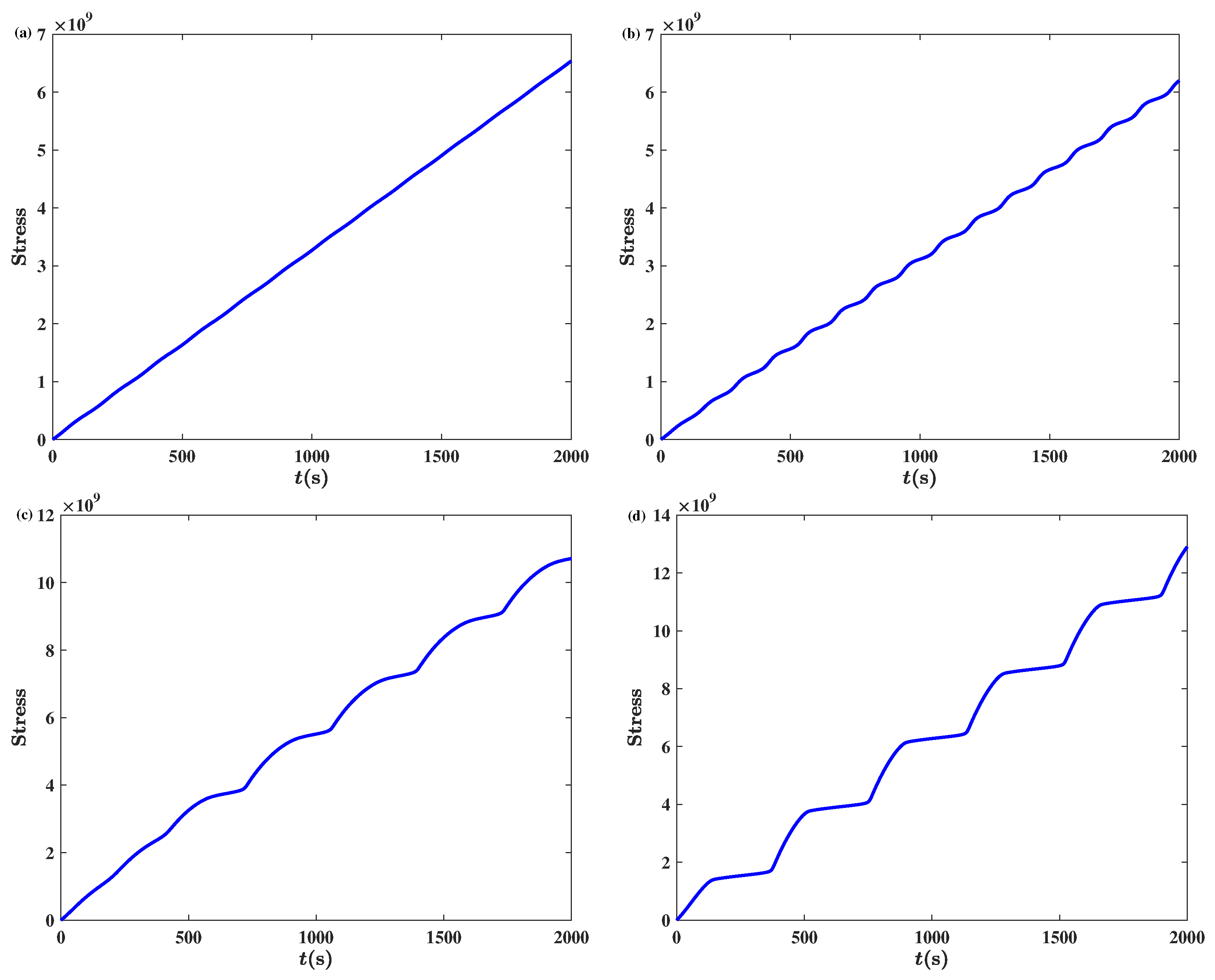Figure 14a,b illustrate the transition of stress-time responses as the fractional order $\alpha$ increases, with other parameters fixed at $a=0.5$, $b=0.01$, $c=0.04$, and $k=1$. Type B behavior (Figure 14b) emerges at $\alpha =0.98$, which exceeds the critical stability threshold (${\alpha }^{*}=0.9068$). This regime exhibits large, irregular serrations, reflecting strong nonlinear interactions and dynamic instability. Figure 14c,d explore the impact of varying the conversion rate parameter k on stress-time patterns at $\alpha =0.98$, with $a=0.4$, $b=0.01$, $c=0.01$. As k decreases from $0.9$ to $0.1$, the transition from mobile to immobile dislocations slows down, leading to the emergence of staircase creep (Type C and D behavior). Notably, the simulated Type A and Type D behaviors observed in Figure 14a,d show qualitative agreement with experimental results reported in Ref. [43], where similar jerky flow and staircase-like yielding patterns are documented in Figure 1(right) and Figure 2(left), respectively. This phenomenon is characterized by increasing amplitude and decreasing frequency, where elastic energy is stored during the horizontal stages and released during vertical jumps, leading to sudden increases in repeated yielding.

7. Conclusions

In this paper, we introduced and analyzed a novel fractional-order Ananthakrishna model, focusing on its stability characteristics, dynamic behaviors, and computational efficiency. The threshold ${\alpha }^{*}$ is analytically determined based on the stability criterion, offering a quantitative indicator of the onset of instability. Combined with bifurcation analysis and Lyapunov exponents, we systematically investigated the stability of equilibrium points, particularly highlighting the extended stability regions compared to the original integer-order model. To facilitate efficient numerical studies, we developed a computationally effective finite difference scheme based on the accelerated L1 method, significantly reducing both computational and storage complexities. Extensive numerical experiments demonstrated that the fractional-order model exhibits rich dynamics, including stable equilibria, periodic solutions, and distinct transitions as fractional orders cross critical thresholds. Moreover, comparisons with conventional numerical methods confirmed the superiority of our accelerated L1 scheme, especially in handling long-term simulations. Finally, we employed the fractional-order framework to reproduce diverse experimental stress-time behaviors associated with repeated yielding, emphasizing its potential utility in capturing realistic physical phenomena. The proposed fractional-order framework is particularly suited for materials and systems exhibiting memory, nonlocality, or anomalous relaxation behavior. Typical examples include viscoelastic materials, dielectric media, and porous structures, where conventional integer-order models may fail to capture the long-term dynamics accurately. These findings suggest broad applicability of the method in complex physical and engineering systems.