Numerical Analysis of a Class of Fractional-Order Nonlinearity Anomalous Subdiffusion Systems

Abstract

Many natural phenomena, such as physical, chemical, and biological processes, can be described using n-coupled nonlinearity anomalous subdiffusion systems. Furthermore, fractional differential equations are a useful tool for modeling practical problems in science because they allow for the incorporation of infinite memory through the consideration of previous states. This paper proposes numerical and analytical techniques for studying n-coupled fractional-order nonlinearity anomalous subdiffusion systems, including the construction of improved implicit difference methods and the discussion of stability and convergence using energy methods. The stability and convergence conditions are determined based on different implicit methods. The obtained conditions are related to the system dimension n. The effectiveness of the theoretical results is demonstrated using two numerical examples.

1. Introduction

Reaction–diffusion equations are commonly used in natural sciences as mathematical models for systems that combine reactions and diffusive motion [1,2,3]. However, the lack of a canonical model for reactions between chemically interacting species that move by anomalous subdiffusion makes it challenging to model such systems in the natural sciences. The type of mesoscopic equation that describes reaction subdiffusion depends on assumptions concerning the microscopic behavior of individual molecules, and the relationship between mesoscopic and microscopic models is yet to be elucidated. This challenge is particularly relevant in cell biology, wherein anomalous subdiffusion is a common phenomenon. Despite these challenges, reaction–diffusion equations remain a valuable mathematical model for understanding systems that combine reactions with diffusive motion. Researchers continue to explore and refine these models to better capture the complexity of natural systems, such as inhomogeneous systems [4], albatross flight [5], physical scenarios [6], and biological cells [7,8].

Fractional differential equations are a valuable tool for modeling practical problems in various fields [9,10], such as biology, chemistry, physics, medicine, and economics. They afford an advantage in that the fractional-order systems have infinite memory, taking into account information from both the current and previous states [11,12]. In the case of anomalous subdiffusive random walkers, the fractional diffusion equation is a better-suited continuum description than the usual diffusion equation. This allows for more accurate modeling and understanding of these systems [13]. Several studies have suggested that the anomalous subdiffusion equation (ASub-DE) provides a more accurate description of these systems than do traditional diffusion equations [14,15,16].

In recent years, the study of anomalous subdiffusion has gained significant attention, leading to the development of numerous numerical methods for solving this problem. These methods include implicit numerical method [17,18], finite difference [19,20,21], finite element [22,23], and Fourier spectral methods [24,25]. The fractional reaction-subdiffusion equation, which describes the behavior of molecular species that react at first-order rates and move subdiffusively, was derived by Lawley [26]. Furthermore, sophisticated techniques such as time-dependent fractional Fokker–Planck equations and stochastically switching evolution equations have been used to derive the necessary equations [27]. Compact finite difference methods are proposed for the fractional diffusion equation and time-fractional subdiffusion equation [28,29,30]. Additionally, various techniques, such as stochastic evolution equations, nonlinear perturbations, and discrete fractional Gronwall inequalities, have been used to discuss the stability, convergence, and regularity of solutions to fractional reaction–subdiffusion equations [31,32,33]. These advances have significantly improved our understanding of anomalous subdiffusion and its role in various fields.

Now, a fractional-order ASub-DE [34] is considered as follows:

$$\begin{array}{c}{\displaystyle \frac{\partial u(t,\widehat{x})}{\partial t}={}_0{}^{R}D_t^{1-q}\{d\frac{\partial u^2(t,\widehat{x})}{\partial {\widehat{x}}^2}+f(t,\widehat{x})\},0<q<1,0<t<T,0<\widehat{x}<L.}\hfill \end{array}$$

A implicit numerical method for solving the fractional-order ASub-DE was proposed by Zhuang et al. [34]. Then, a modified fractional-order ASub-DE with nonlinear source term proposed by Liu et al. [35] can be given as

$$\begin{array}{c}{\displaystyle \frac{\partial u(t,\widehat{x})}{\partial t}=({}_0{}^{R}D_t^{1-q_1}{d}_1+{}_0{}^{R}D_t^{1-q_2}{d}_2)\{\frac{\partial u^2(t,\widehat{x})}{\partial {\widehat{x}}^2}+f(t,\widehat{x})\}+g(u,t,\widehat{x}),}\hfill \\ 0<q_1<1,0<q_1<1,0<t<T,0<\widehat{x}<L.\hfill \end{array}$$

In contrast with the approach in [34], the extended implicit difference method in [35] is constructed using an energy method. Further, the initial boundary value problem of the fractional-order ASub-DE was examined by Zhang et al. [36].

$$\begin{array}{c}{\displaystyle \frac{\partial u(t,\widehat{x})}{\partial t}={}_0{}^{R}D_t^{1-q}\{d\frac{\partial u^2(t,\widehat{x})}{\partial {\widehat{x}}^2}\}+f(t,\widehat{x}),0<q<1,0<t<T,0<\widehat{x}<L.}\hfill \end{array}$$

A Crank–Nicolson-type difference scheme was proposed for solving the fractional-order subdiffusion equation and analyzing the truncation error [36].

Furthermore, two-dimensional time fractional-order ASub-DEs were discussed in [37,38,39]. Roul and Rohil [38] analyzed the convergence and stability of two-dimensional time fractional-order ASub-DEs based on a compact alternating direction implicit finite difference scheme. Using the high-order time-stepping scheme on graded meshes, Wei et al. [39] analyzed a class of two-dimensional time fractional-order ASub-DEs with variable coefficients, which was considered so as to handle the weak for spatial discretization. Xie et al. [40] applied a Galerkin finite element scheme coupled with implicit and explicit algorithm for 2D nonlinear time fractional ASub-DEs. Three-dimensional variable-order time fractional-order ASub-DEs are considered based on discrete shifted Hahn polynomials and their operational matrices [41]. An alternating direction implicit difference method is given to solve the two-dimensional time fractional-order ASub-DEs based on discrete fractional Gronwall inequality [42,43]. Convergence and stability analyses of time fractional-order ASub-DEs are proposed by means of a high-order alternating direction implicit compact finite difference scheme [44,45].

Many natural systems, such as biological, ecological, and physical systems, are coupled systems, are composed of two or more interconnected elements that interact with each other in a complex way. In a coupled system, the behavior of each component is influenced by the behavior of the other components, leading to self-organization and emergent phenomena. Analysis of the behavior of each individual component in the system and how they interact with each other can yield deep insights into the behavior of the system as a whole. Overall, studying coupled systems is essential for understanding and effectively managing many complex natural phenomena. As regards the reaction front in an $A+B\to C$ reaction–subdiffusion process, the two coupled fractional reaction–subdiffusion equations are given as follows [46,47]:

$$\left\{\begin{array}{c}{\displaystyle \frac{\partial u_1(t,\widehat{x})}{\partial t}={}_0{}^{R}D_t^{1-q}\{d\frac{\partial u_1^2(t,\widehat{x})}{\partial {\widehat{x}}^2}\}-a_1{u}_1(t,\widehat{x})u_2(t,\widehat{x}),}\hfill \\ \\ {\displaystyle \frac{\partial u_2(t,\widehat{x})}{\partial t}={}_0{}^{R}D_t^{1-q}\{d\frac{\partial u_2^2(t,\widehat{x})}{\partial {\widehat{x}}^2}\}-a_2{u}_1(t,\widehat{x})u_2(t,\widehat{x}),}\hfill \end{array}\right.$$

where $0<q<1,0<t<T,0<\widehat{x}<L.$

In this paper, a system of n-coupled fractional reaction–subdiffusion equations is proposed as

$$\begin{array}{c}{\displaystyle \frac{\partial u_i(t,\widehat{x})}{\partial t}={}_0{}^{R}D_t^{1-q}\{d_i\frac{\partial u_i^2(t,\widehat{x})}{\partial {\widehat{x}}^2}+I_i(t,\widehat{x})\}-a_i{u}_i(t,\widehat{x})+\sum _{j=1}^n{b}_{ij}{f}_j(u_j(t,\widehat{x})),}\hfill \\ t>0,i=1,2,\dots ,n.\hfill \end{array}$$

While many effective methods have been suggested for solving fractional-order ASub-DEs, there are currently few studies on the numerical analysis of n-coupled fractional-order ASub-DEs. Therefore, it is crucial to examine both analytical techniques and numerical approaches for n-coupled nonlinear fractional-order ASub-DEs so as to gain valuable insights into the behavior and properties of these complex systems and develop more accurate and efficient solutions for a wide range of applications.

In this paper, we present the numerical analysis and analytical techniques of n-coupled fractional-order nonlinearity ASub-DEs. Based on the implicit numerical method in [34,35], we demonstrate the improvement in its application for numerical analysis of n-coupled fractional-order nonlinearity ASub-DEs. The stability and convergence are investigated by the improved energy methods. Furthermore, three improved implicit difference methods are constructed. Two of these methods are well-suited for numerical analysis. However, one of the methods is not effective for stability and convergence analysis. In addition, the obtained conditions of stability and convergence are related to model dimension n, highlighting the importance of temporal difference related to the model dimension. Lastly, the effectiveness of the obtained theoretical results using two numerical examples is demonstrated.

The paper is organized as follows. Section 2 presents some preliminaries and the model description. In Section 3, three implicit numerical methods for the n-coupled fractional-order nonlinearity ASub-DEs are first proposed. Thereafter, the stability and convergence of the improved implicit numerical method are proposed. Section 4 provides two computational examples to validate the given theorems. Finally, Section 5 presents our conclusions and related discussion.

2. Model Description

2.1. Definitions and Lemmas

In this section, we introduce certain elementary notations and present some results on fractional-order systems. These notations and results are used in numerical analysis of a class of fractional-order nonlinearity ASub-DEs.

Definition 1

([10]). Riemann–Liouville fractional derivative of a function f is defined as

$${}_0{}^{R}D_t^{q}f(t,\widehat{x})={\displaystyle \frac{1}{\Gamma (1-q)}}{\displaystyle \frac{d}{dt}}{\int }_0^t{\displaystyle \frac{f(s,\widehat{x})}{{(t-s)}^q}}ds,$$

where $0<q<1$ and $\Gamma (·)$ is the Gamma function.

Definition 2

([10]). Riemann–Liouville fractional integral of a function f is defined as

$$I_t^{q}f(t,\widehat{x})={\displaystyle \frac{1}{\Gamma (q)}}{\int }_0^t{(t-s)}^{q-1}f(s,\widehat{x})ds,(q>0).$$

Some properties of the Riemann–Liouville fractional derivative and fractional integral are obtained as follows [48]:

Property 1.

${\displaystyle {}_0{}^{R}D_t^q(af(t,\widehat{x})+bg(t,\widehat{x}))=a{}_0{}^{R}D_t^{q}f(t,\widehat{x})+b{}_0{}^{R}D_t^{q}g(t,\widehat{x})}$, where $a,b,q\in \mathbb{R}$.

Property 2.

${\displaystyle {}_0{}^{R}D_t^p{I}_t^{q}f(t,\widehat{x})={}_0{}^{R}D_t^{p-q}f(t,\widehat{x})}$, where $p,q\in {\mathbb{R}}^{+}.$

Let $f(t)$ be a continuous-differential function in $[0,T]$. Considering a uniform grid of $[0,T]$, $\sigma =T/N,t_k=k\sigma$, and $k=0,1,\dots ,N$. Using the fractional integral, the following results:

$$I_0^{q}f(t_k)={\displaystyle \frac{1}{\Gamma (q)}}\sum _{j=1}^k{\int }_{t_{j-1}}^{t_j}{\displaystyle \frac{f(\xi )}{t_k-\xi }}d\xi .$$

Lemma 1

([34]). If $f(t)\in C^1[0,T]$ and $k=0,1,\dots ,N$, $I_0^{q}f(t_k)$ can be approximated as

$$I_0^{q}f(t_k)={\displaystyle \frac{{\sigma }^q}{\Gamma (1+q)}}\sum _{j=0}^{k-1}{b}_j^{q}f(t_{k-j})+R_k^1,$$

(1)

where $R_k^1\le C\sigma$, C is a constant, and $b_j^q={(j+1)}^q-j^q$.

Lemma 2

([34]). If $f(t)\in C^2[0,T]$, $k=0,1,\dots ,N$,

$${\nabla }_t{I}_0^{q}f(t_k)={\displaystyle \frac{{\sigma }^q}{\Gamma (1+q)}}[f(t_k)-\sum _{j=1}^{k-1}(b_{j-1}^q-b_j^q)f(t_{k-j})]+R_k^2,$$

(2)

where $R_k^2\le C(b_{k-1}^q{\sigma }^{1+q}+{\sigma }^2)$, C is a constant, and $b_j^q={(j+1)}^q-j^q$.

Lemma 3

([34,35]). Suppose ${\displaystyle \parallel F^k{\parallel }_2^2=\sum _{i=1}^{M-1}{|f_i^k|}^{2}h}$, ${\displaystyle |F^k{|}_{\infty }=\underset{1\le i\le M-1}{max}|f_i^k|}$. Then,

$$\parallel F^k{\parallel }_2^2\le L\parallel F^k{\parallel }_{\infty }^2\le {\displaystyle \frac{L^2}{2h^2}}[h|f_1^k{|}^2+\parallel {\Delta }_x{F}^k{\parallel }_2^2],$$

(3)

where h is a step size, and L is the interval length.

2.2. Model Description

Consider the following fractional-order nonlinearity ASub-DE:

$$\begin{array}{c}{\displaystyle \frac{\partial u_i(t,\widehat{x})}{\partial t}={}_0{}^{R}D_t^{1-q}\{d_i\frac{\partial u_i^2(t,\widehat{x})}{\partial {\widehat{x}}^2}+I_i(t,\widehat{x})\}-a_i{u}_i(t,\widehat{x})+\sum _{j=1}^n{b}_{ij}{f}_j(u_j(t,\widehat{x})),}\hfill \\ i=1,2,\dots ,n,t>0,\hfill \end{array}$$

(4)

where $q\in (0,1)$, n corresponds to the number of units; $u_i(t,\widehat{x})$ corresponds to the ith unit at time t and space $\widehat{x}$; $f_j(·)$ denotes j nonlinearity functions at time t and in space $\widehat{x}$; $d_i$ denotes the transmission diffusion operator along the ith unit; $a_i$ represents the rate, $b_{ij}$ denotes the synaptic connection weight of the unit j to the unit i at time t and in space $\widehat{x}$; and $I_i(t,\widehat{x})$ is the control input vector.

We consider Equation (4) subject to the following Dirichlet boundary conditions:

$$u_i(t,\widehat{x})=0,t\in [0,\infty ],\widehat{x}\in \partial \Omega$$

(5)

and initial conditions

$$u_i(0,\widehat{x})={\varphi }_{0i}(0,\widehat{x}),\widehat{x}\in \Omega ,$$

(6)

where $i=1,2,\dots ,n$, and ${\varphi }_{0i}(0,\widehat{x})$(${\varphi }_{0i}={({\varphi }_{01},{\varphi }_{02},\dots ,{\varphi }_{0n})}^T)$ denote a real-valued continuous function defined on $\Omega$.

Remark 1.

If the fractional-order $q=1$, the Equation (4) is a class of integral-order nonlinearity reaction–diffusion systems:

$$\begin{array}{c}{\displaystyle \frac{\partial u_i(t,\widehat{x})}{\partial t}=d_i\frac{\partial u_i^2(t,\widehat{x})}{\partial {\widehat{x}}^2}-a_i{u}_i(t,\widehat{x})+\sum _{j=1}^n{b}_{ij}{f}_j(u_j(t,\widehat{x}))+I_i(t,\widehat{x}),i=1,2,\dots ,n.}\hfill \end{array}$$

In addition, when $n=1$ and $a=0$, the Equation (4) becomes

$$\begin{array}{c}{\displaystyle \frac{\partial u(t,\widehat{x})}{\partial t}={}_0{}^{R}D_t^{1-q}\{d\frac{\partial u^2(t,\widehat{x})}{\partial {\widehat{x}}^2}+I(t,\widehat{x})\}+bf(u(t,\widehat{x})).}\hfill \end{array}$$

Then, the Equation (4) is similar to that presented in [35].

3. Main Results

In this section, improved implicit difference methods are developed for the fractional-order nonlinearity ASub-DEs. Furthermore, using the improved energy methods, the stability and convergence are discussed.

3.1. Formulation of Numerical Method

According to [34,35], the key approaches of implicit difference methods can be summarized in the Lemmas 1 and 2. The formulation of the improved implicit difference methods of system (4) are given based on the Lemmas 1 and 2.

Consider a uniform grid $t_k=\sigma k:k=0,1,\dots ,N$, where N is an integer and $\sigma =T/N$. Additionally, ${\widehat{x}}_{\widehat{i}}=a+\widehat{i}h,\widehat{i}=1,2,\dots ,M$. Let ${\delta }_{\widehat{x}}^{2}u(\widehat{x},t)=u(\widehat{x}+h,t)-2u(\widehat{x},t)+u(\widehat{x}-h,t)$.

Using a discrete form of Equation (4), we get

$$\begin{array}{c}{\displaystyle \frac{u_i({\widehat{x}}_{\widehat{i}},t_{k+1})-u_i({\widehat{x}}_{\widehat{i}},t_k)}{\sigma }}={}_0{}^{R}D_t^{1-q}\{d_i{\displaystyle \frac{\partial u_i^2(t,\widehat{x})}{\partial {\widehat{x}}^2}}+I_i(t,\widehat{x})\}{|}_{({\widehat{x}}_{\widehat{i}},t_{k+1})}-a_i{u}_i(t,\widehat{x}){|}_{({\widehat{x}}_{\widehat{i}},t_{k+1})}\hfill \\ {\displaystyle +\sum _{j=1}^n{b}_{ij}{f}_j(u_j(t,\widehat{x})){|}_{({\widehat{x}}_{\widehat{i}},t_{k+1})},t>0,i=1,2,\dots ,n.}\hfill \end{array}$$

(7)

Based on Lemmas 1 and 2, we can get

$$\begin{array}{c}{\nabla }_t{I}_0^q\{d_i{\displaystyle \frac{\partial u_i^2(t,\widehat{x})}{\partial {\widehat{x}}^2}}+I_i(t,\widehat{x})\}{|}_{({\widehat{x}}_{\widehat{i}},t_{k+1})}={\displaystyle \frac{{\sigma }^q}{\Gamma (1+q)}}[\{d_i{\displaystyle \frac{\partial u_i^2(t,\widehat{x})}{\partial {\widehat{x}}^2}}+I_i(t,\widehat{x})\}{|}_{({\widehat{x}}_{\widehat{i}},t_{k+1})}\hfill \\ {\displaystyle -\sum _{\widehat{j}=1}^k(b_{\widehat{j}-1}^q-b_{\widehat{j}}^q)\{d_i\frac{\partial u_i^2(t,\widehat{x})}{\partial {\widehat{x}}^2}+I_i(t,\widehat{x})\}{|}_{({\widehat{x}}_{\widehat{i}},t_{k+1})}]+R_{i(k+1)}^1,}\hfill \end{array}$$

(8)

where $|R_{ik+1}^1| \le C_i^1(b_{k-1}^q{\sigma }^{1+q}+{\sigma }^2)$, $C_i^1$ is a constant, and $b_j^q={(j+1)}^q-j^q$. Then, Equation (8) becomes

$$\begin{array}{c}{u}_i({\widehat{x}}_{\widehat{i}},t_{k+1})=u_i({\widehat{x}}_{\widehat{i}},t_k)+{\displaystyle \frac{{\sigma }^q}{\Gamma (1+q)}}\{d_i{\displaystyle \frac{\partial u_i^2(t,\widehat{x})}{\partial {\widehat{x}}^2}}{|}_{({\widehat{x}}_{\widehat{i}},t_{k+1})}+I_i({\widehat{x}}_{\widehat{i}},t_{k+1})\}\hfill \\ {\displaystyle +\frac{{\sigma }^q}{\Gamma (1+q)}\sum _{\widehat{j}=1}^k(b_{\widehat{j}-1}^q-b_{\widehat{j}}^q)\{d_i\frac{\partial u_i^2(t,\widehat{x})}{\partial {\widehat{x}}^2}{|}_{({\widehat{x}}_{\widehat{i}},t_{k+1-\widehat{j}})}+I_i({\widehat{x}}_{\widehat{i}},t_{k+1-\widehat{j}})\}}\hfill \\ {\displaystyle -\sigma a_i{u}_i({\widehat{x}}_{\widehat{i}},t_{k+1})+\sigma \sum _{j=1}^n{b}_{ij}{f}_j(u_j({\widehat{x}}_{\widehat{i}},t_k))+R_{i(k+1)}^1+R_{i(k+1)}^2.}\hfill \end{array}$$

(9)

According to [34,35], if $f_i(u)$ is a continuously differentiable function and $u_i(\widehat{x},t)\in C_{\widehat{x},t}^{4,2}([0,L]\times (0,T])$, we have

$$\begin{array}{c}{f}_i(u_i({\widehat{x}}_{\widehat{i}},t_{k+1}))-f_i(u_i({\widehat{x}}_{\widehat{i}},t_k))=f_i^{\prime }({\eta }_k)(u_i({\widehat{x}}_{\widehat{i}},t_{k+1})-u_i({\widehat{x}}_{\widehat{i}},t_k))\hfill \\ =f_i^{\prime }({\eta }_k){\displaystyle \frac{\partial u_i}{\partial t}}({\widehat{x}}_{\widehat{i}},{\eta }_k^{\prime })(t_{k+1}-t_k)=f_i^{\prime }({\eta }_k){\displaystyle \frac{\partial u_i}{\partial t}}({\widehat{x}}_{\widehat{i}},{\eta }_k^{\prime })\sigma .\hfill \end{array}$$

(10)

Hence, we obtain $|R_{i(k+1)}^2| \le C_i^2{\sigma }^2$.

Furthermore, when $u_i(\widehat{x},t)\in C_{\widehat{x},t}^{4,2}([0,L]\times (0,T])$,

$${\displaystyle \frac{\partial u_i^2({\widehat{x}}_{\widehat{i}},t_{k+1}))}{\partial {\widehat{x}}^2}}={\displaystyle \frac{1}{h^2}}{\delta }_{\widehat{x}}^2{u}_i({\widehat{x}}_{\widehat{i}},t_{k+1})+R_{i(k+1)}^3,$$

where $|R_{i(k+1)}^3| \le C_i^3{h}^2$.

From the obtained results, the following expression can be derived:

$$\begin{array}{c}{u}_i({\widehat{x}}_{\widehat{i}},t_{k+1})=u_i({\widehat{x}}_{\widehat{i}},t_k)+{\displaystyle \frac{{\sigma }^q}{\Gamma (1+q)}}\{d_i{\displaystyle \frac{1}{h^2}}{\delta }_x^2{u}_i({\widehat{x}}_{\widehat{i}},t_{k+1})+I_i({\widehat{x}}_{\widehat{i}},t_{k+1})+R_{i(k+1)}^3\}\hfill \\ {\displaystyle +\frac{{\sigma }^q}{\Gamma (1+q)}\sum _{\widehat{j}=1}^k(b_{\widehat{j}-1}^q-b_{\widehat{j}}^q)\{d_i\frac{1}{h^2}{\delta }_{\widehat{x}}^2{u}_i({\widehat{x}}_{\widehat{i}},t_{k+1-\widehat{j}}))+I_i({\widehat{x}}_{\widehat{i}},t_{k+1-\widehat{j}})+R_{i(k+1)}^3\}}\hfill \\ {\displaystyle -\sigma a_i{u}_i({\widehat{x}}_{\widehat{i}},t_{k+1})+\sigma \sum _{j=1}^n{b}_{ij}{f}_j(u_j({\widehat{x}}_{\widehat{i}},t_k))+R_{i(k+1)}^2+R_{i(k+1)}^1.}\hfill \end{array}$$

(11)

Let $r_1={\displaystyle \frac{{\sigma }^q}{\Gamma (q+1)h^2}}$, and $r_2={\displaystyle \frac{{\sigma }^q}{\Gamma (q+1)}}$. Then, we have

$$\begin{array}{c}{\displaystyle u_i({\widehat{x}}_{\widehat{i}},t_{k+1})=u_i({\widehat{x}}_{\widehat{i}},t_k)+r_1{d}_i{\delta }_{\widehat{x}}^2{u}_i({\widehat{x}}_{\widehat{i}},t_{k+1})-\sigma a_i{u}_i({\widehat{x}}_{\widehat{i}},t_{k+1})+\sigma \sum _{j=1}^n{b}_{ij}{f}_j(u_j({\widehat{x}}_{\widehat{i}},t_k))}\hfill \\ {\displaystyle +r_2{I}_i({\widehat{x}}_{\widehat{i}},t_{k+1})+r_2{R}_{i(k+1)}^3-\sum _{\widehat{j}=0}^{k-1}(b_{\widehat{j}}^q-b_{\widehat{j}+1}^q)r_1{d}_i{\delta }_{\widehat{x}}^2{u}_i({\widehat{x}}_{\widehat{i}},t_{k-\widehat{j}})}\hfill \\ {\displaystyle -\sum _{\widehat{j}=0}^{k-1}(b_{\widehat{j}}^q-b_{\widehat{j}+1}^q)r_2{I}_i({\widehat{x}}_{\widehat{i}},t_{k-\widehat{j}})-\sum _{\widehat{j}=0}^{k-1}(b_{\widehat{j}}^q-b_{\widehat{j}+1}^q)r_2{R}_{i(k+1)}^3+R_{i(k+1)}^2.}\hfill \end{array}$$

(12)

Let total error of Equation (12) be $R_i^{k+1}$. Notably, ${\displaystyle \sum _{\widehat{j}=0}^{k-1}(b_{\widehat{j}}^q-b_{\widehat{j}+1}^q)=b_0^q-b_k^q=1-b_k^q}$, then

$$\begin{array}{c}{\displaystyle R_i^{k+1}=r_2{R}_{i(k+1)}^3-\sum _{\widehat{j}=0}^{k-1}(b_{\widehat{j}}^q-b_{\widehat{j}+1}^q)r_2{R}_{i(k+1)}^3+R_{i(k+1)}^2+R_{i(k+1)}^1}\hfill \\ {\displaystyle =(1-\sum _{\widehat{j}=0}^{k-1}(b_{\widehat{j}}^q-b_{\widehat{j}+1}^q))r_2{R}_{i(k+1)}^3+R_{i(k+1)}^2+R_{i(k+1)}^1}\hfill \\ =b_k^q{r}_2{R}_{i(k+1)}^3+R_{i(k+1)}^2+R_{i(k+1)}^1.\hfill \end{array}$$

According to [34], there exists a positive constant $\overline{C}>0$ such that

$$\sigma \le \overline{C}{b}_k^q{\sigma }^{1+q}.$$

On the basis of the obtained expression, we have

$$\begin{array}{c}{\displaystyle |R_i^{k+1}|\le b_k^q\frac{{\sigma }^q}{\Gamma (1+q)}{C}_i^3{h}^2+C_i^2{\sigma }^2+C_i^1(b_k^q{\sigma }^{1+q}+{\sigma }^2)}\hfill \\ {\displaystyle =b_k^q\frac{{\sigma }^q}{\Gamma (1+q)}{C}_i^3{h}^2+(C_i^1+C_i^2){\sigma }^2+C_i^1{b}_k^q{\sigma }^{1+q}}\hfill \\ {\displaystyle \le b_k^q\frac{{\sigma }^q}{\Gamma (1+q)}{C}_i^3{h}^2+(C_i^1+C_i^2)\overline{C}{b}_k^q{\sigma }^{1+q}\sigma +C_i^1{b}_k^q{\sigma }^{1+q}}\hfill \\ {\displaystyle \le b_k^q{\widehat{C}}_i{\sigma }^q(h^2+\sigma +{\sigma }^2)}\hfill \\ \le 2b_k^q{\widehat{C}}_i{\sigma }^q(h^2+\sigma ),\hfill \end{array}$$

where ${\widehat{C}}_i=\mathit{max}\{\frac{C_i^3}{\Gamma (1+q)}, (C_i^1+C_i^2)\overline{C}, C_i^1\}$.

The implicit finite difference scheme of Equation (4) can now be derived as follows:

$$\begin{array}{c}{\displaystyle u_i({\widehat{x}}_{\widehat{i}},t_{k+1})=u_i({\widehat{x}}_{\widehat{i}},t_k)+r_1{d}_i{\delta }_{\widehat{x}}^2{u}_i({\widehat{x}}_{\widehat{i}},t_{k+1})-\sigma a_i{u}_i({\widehat{x}}_{\widehat{i}},t_{k+1})+\sigma \sum _{j=1}^n{b}_{ij}{f}_j(u_j({\widehat{x}}_{\widehat{i}},t_k))}\hfill \\ {\displaystyle +r_2{I}_i({\widehat{x}}_{\widehat{i}},t_{k+1})-\sum _{\widehat{j}=0}^{k-1}(b_{\widehat{j}}^q-b_{\widehat{j}+1}^q)r_1{d}_i{\delta }_{\widehat{x}}^2{u}_i({\widehat{x}}_{\widehat{i}},t_{k-\widehat{j}})}\hfill \\ {\displaystyle -\sum _{\widehat{j}=0}^{k-1}(b_{\widehat{j}}^q-b_{\widehat{j}+1}^q)r_2{I}_i({\widehat{x}}_{\widehat{i}},t_{k-\widehat{j}})+R_i^{k+1},}\hfill \end{array}$$

(13)

where $|R_i^{k+1}| \le 2b_k^q{\widehat{C}}_i{\sigma }^q(h^2+\sigma ),i=1,2,\dots ,n$.

Let ${\delta }_{\widehat{x}}^{2}u({\widehat{x}}_{\widehat{i}},t_{k+1})=u_{\widehat{i}+1}^{k+1}-2u_{\widehat{i}}^{k+1}+u_{\widehat{i}-1}^{k+1}$. So, the implicit finite difference scheme can be written as follows:

$$\begin{array}{c}{\displaystyle {}^{i}u_{\widehat{i}}^{k+1}={}^{i}u_{\widehat{i}}^k+r_1{d}_i{(}^i{u}_{\widehat{i}+1}^{k+1}-2{(}^i{u}_{\widehat{i}}^{k+1}){+}^i{u}_{\widehat{i}-1}^{k+1})-\sigma a_i{}^{i}u_{\widehat{i}}^{k+1}+\sigma \sum _{j=1}^n{b}_{ij}{f}_j{(}^j{u}_{\widehat{i}}^k)}\hfill \\ {\displaystyle +r_2{}^{i}I_{\widehat{i}}^{k+1}+\sum _{\widehat{j}=0}^{k-1}(b_{\widehat{j}+1}^q-b_{\widehat{j}}^q)r_1{d}_i{\delta }_{\widehat{x}}^2{(}^i{u}_{\widehat{i}}^{k-\widehat{j}})+\sum _{\widehat{j}=0}^{k-1}(b_{\widehat{j}}^q-b_{\widehat{j}+1}^q)r_2{}^{i}I_{\widehat{i}}^{k-\widehat{j}}.}\hfill \end{array}$$

(14)

Furthermore,

$$\begin{array}{c}-r_1{d}_i{(}^i{u}_{\widehat{i}+1}^{k+1})+{(1+2r_1{d}_i+\sigma a_i)}^i{u}_{\widehat{i}}^{k+1}-r_1{d}_i{(}^i{u}_{\widehat{i}-1}^{k+1})\hfill \\ {\displaystyle ={}^{i}u_{\widehat{i}}^k+\sigma \sum _{j=1}^n{b}_{ij}{f}_j{(}^j{u}_{\widehat{i}}^k)+\sum _{\widehat{j}=0}^{k-1}(b_{\widehat{j}+1}^q-b_{\widehat{j}}^q)r_1{d}_i{\delta }_{\widehat{x}}^2({}^{i}u_{\widehat{i}}^{k-\widehat{j}})+r_2{}^{i}I_{\widehat{i}}^{k+1}+\sum _{\widehat{j}=0}^{k-1}(b_{\widehat{j}+1}^q-b_{\widehat{j}}^q)r_2{}^{i}I_{\widehat{i}}^{k-\widehat{j}}.}\hfill \end{array}$$

(15)

Equation (15) can be rewritten in the matrix form as follows:

$$\begin{array}{c}{A}_i{U}_i^{k+1}=U_i^k+r_1{d}_i{V}_i^k+\sigma F_i^k+r_2{I}_i^{k+1},i=1,2,\dots ,n,\hfill \end{array}$$

(16)

where

$$A_i=\left(\begin{array}{cccccc}1+2r_1{d}_i+\sigma a_i& -r_1{d}_i& 0& \dots & 0& 0\\ -r_1{d}_i& 1+2r_1{d}_i+\sigma a_i& -r_1{d}_i& \dots & 0& 0\\ 0& -r_1{d}_i& 1+2r_1{d}_i+\sigma a_i& \dots & 0& 0\\ \dots & \dots & \dots & \dots & \dots & \dots \\ 0& 0& 0& \dots & 1+2r_1{d}_i+\sigma a_i& -r_1{d}_i\\ 0& 0& 0& \dots & -r_1{d}_i& 1+2r_1{d}_i+\sigma a_i\end{array}\right),$$

$U_i^k={{[}^i{u}_1^k{,}^i{u}_2^k,\dots {,}^i{u}_{M-1}^k]}^T$,

• ${\displaystyle V_i^k=[\sum _{\widehat{j}=0}^{k-1}(b_{\widehat{j}+1}^q-b_{\widehat{j}}^q)r_1{d}_i{\delta }_{\widehat{x}}^2({}^{i}u_1^{k-\widehat{j}}),\sum _{\widehat{j}=0}^{k-1}(b_{\widehat{j}+1}^q-b_{\widehat{j}}^q)r_1{d}_i{\delta }_{\widehat{x}}^2({}^{i}u_2^{k-\widehat{j}})\dots ,\sum _{\widehat{j}=0}^{k-1}(b_{\widehat{j}+1}^q-b_{\widehat{j}}^q)r_1{d}_i{\delta }_{\widehat{x}}^2({}^{i}u_{M-1}^{k-\widehat{j}}){]}^T}$,
• ${\displaystyle F_i^k=[\sum _{j=1}^n{b}_{ij}{f}_j{(}^j{u}_1^k),\sum _{j=1}^n{b}_{ij}{f}_j{(}^j{u}_2^k),\dots ,\sum _{j=1}^n{b}_{ij}{f}_j{(}^j{u}_{M-1}^k){]}^T}$,
• ${\displaystyle I_i^{k+1}={[}^i{I}_1^{k+1}+\sum _{\widehat{j}=0}^{k-1}(b_{\widehat{j}+1}^q-b_{\widehat{j}}^q){}^{i}I_1^{k-\widehat{j}}{,}^i{I}_2^{k+1}+\sum _{\widehat{j}=0}^{k-1}(b_{\widehat{j}+1}^q-b_{\widehat{j}}^q){}^{i}I_2^{k-\widehat{j}},\dots {,}^i{I}_{M-1}^{k+1}+\sum _{\widehat{j}=0}^{k-1}(b_{\widehat{j}+1}^q-b_{\widehat{j}}^q){}^{i}I_{M-1}^{k-\widehat{j}}{]}^T}$.

When $k=0$

$$\begin{array}{c}{A}_i{U}_i^1=U_i^0+\sigma F_i^0+r_2{I}_i^1,\hfill \end{array}$$

(17)

where

$U_i^0={[{\varphi }_{0i}(0,h),{\varphi }_{0i}(0,2h),\dots ,{\varphi }_{0i}(0,(M-1)h)]}^T$,

${\displaystyle F_i^0=[\sum _{j=1}^n{b}_{ij}{f}_j({\varphi }_{0j}(0,h)),\sum _{j=1}^n{b}_{ij}{f}_j{(}^j{\varphi }_{0j}(0,2h)),\dots ,\sum _{j=1}^n{b}_{ij}{f}_j{(}^j{\varphi }_{0j}(0,(M-1)h)){]}^T}$,

$I_i^1={[}^i{I}_1^1,{}^{i}I_2^1,\dots ,{}^{i}I_{M-1}^1{]}^T$.

Remark 2.

Notably, the right side of the implicit finite difference scheme equation in Equation (16) has the term $\sigma a_i{u}_i({\widehat{x}}_{\widehat{i}},t_{k+1})$. If we replace $\sigma a_i{u}_i({\widehat{x}}_{\widehat{i}},t_{k+1})$ with $\sigma a_i{u}_i({\widehat{x}}_{\widehat{i}},t_k)$ by using similar techniques, we have

$$\begin{array}{c}{A}_i{U}_i^{k+1}=(1-\sigma a_i)U_i^k+r_1{d}_i{V}_i^k+\sigma F_i^k+r_2{I}_i^{k+1}+R_i^{k+1},\hfill \end{array}$$

(18)

where

$$A_i=\left(\begin{array}{cccccc}1+2r_1{d}_i& -r_1{d}_i& 0& \dots & 0& 0\\ -r_1{d}_i& 1+2r_1{d}_i& -r_1{d}_i& \dots & 0& 0\\ 0& -r_1{d}_i& 1+2r_1{d}_i& \dots & 0& 0\\ \dots & \dots & \dots & \dots & \dots & \dots \\ 0& 0& 0& \dots & 1+2r_1{d}_i& -r_1{d}_i\\ 0& 0& 0& \dots & -r_1{d}_i& 1+2r_1{d}_i\end{array}\right),$$

and $|R_i^{k+1}|\le 2b_k^q{\widehat{C}}_i{\sigma }^q(h^2+\sigma )$.

Remark 3.

Due to the coupling effect of n-coupled nonlinearity anomalous subdiffusion systems, where they mutually influence and interact with each other, their stability and convergence are also interdependent. Thus, improved implicit difference methods of Equations (16) and (18) are presented to effectively addresses this issue. Our results extend the given results in [34,35] to n-coupled nonlinearity anomalous subdiffusion systems.

3.2. Stability Analysis

Theorem 1.

If the discretization matrix $A_i(i=1,2,\dots ,n)$ is invertible, Equation (16) has a unique solution.

Suppose that ${}^i\tilde{u}_{\widehat{i}}^k(i=0,1,2,\dots ,n)$ is the approximate solution of Equation (16) and it satisfies

$$\begin{array}{c}{\displaystyle {}^i\tilde{u}_{\widehat{i}}^{k+1}={}^i\tilde{u}_{\widehat{i}}^k+r_1{d}_i{(}^i{\tilde{u}}_{\widehat{i}+1}^{k+1}-2{(}^i{\tilde{u}}_{\widehat{i}}^{k+1}){+}^i{\tilde{u}}_{\widehat{i}-1}^{k+1})-\sigma a_i{}^i\tilde{u}_{\widehat{i}}^{k+1}+\sigma \sum _{j=1}^n{b}_{ij}{f}_j{(}^j{\tilde{u}}_{\widehat{i}}^k)}\hfill \\ {\displaystyle +r_2{}^{i}I_{\widehat{i}}^{k+1}+\sum _{\widehat{j}=0}^{k-1}(b_{\widehat{j}+1}^q-b_{\widehat{j}}^q)r_1{d}_i{\delta }_{\widehat{x}}^2{(}^i{\tilde{u}}_{\widehat{i}}^{k-\widehat{j}})+\sum _{\widehat{j}=0}^{k-1}(b_{\widehat{j}+1}^q-b_{\widehat{j}}^q)r_2{}^{i}I_{\widehat{i}}^{k-\widehat{j}}.}\hfill \end{array}$$

(19)

Let the rounding error ${}^i\epsilon _{\widehat{i}}^k={}^i\tilde{u}_{\widehat{i}}^k-{}^{i}u_{\widehat{i}}^k$. Then, it satisfies

$$\begin{array}{c}{\displaystyle {}^i\epsilon _{\widehat{i}}^{k+1}={}^i\epsilon _{\widehat{i}}^k+r_1{d}_i{(}^i{\epsilon }_{\widehat{i}+1}^{k+1}-2{(}^i{\epsilon }_{\widehat{i}}^{k+1}){+}^i{\epsilon }_{\widehat{i}-1}^{k+1})-\sigma a_i{}^i\epsilon _{\widehat{i}}^{k+1}+\sum _{\widehat{j}=0}^{k-1}(b_{\widehat{j}+1}^q-b_{\widehat{j}}^q)r_1{d}_i{\delta }_{\widehat{x}}^2{(}^i{\epsilon }_{\widehat{i}}^{k-\widehat{j}})}\hfill \\ {\displaystyle +\sigma \sum _{j=1}^n{b}_{ij}[f_j{(}^j{\tilde{u}}_{\widehat{i}}^k)-f_j{(}^j{u}_{\widehat{i}}^k)].}\hfill \end{array}$$

(20)

Take $f(u)$ be a continuously differentiable function. Then, we have

$$\begin{array}{c}{f}_j{(}^j{\tilde{u}}_{\widehat{i}}^k)-f_j{(}^j{u}_{\widehat{i}}^k)=f_j^{\prime }{(}^j{\zeta }_{\widehat{i}}^k){(}^j{\tilde{u}}_{\widehat{i}}^k{-}^j{u}_{\widehat{i}}^k))=f_j^{\prime }{(}^j{\zeta }_{\widehat{i}}^k){(}^j{\epsilon }_{\widehat{i}}^k),\hfill \end{array}$$

(21)

where ${}^j\zeta _{\widehat{i}}^k$ is between ${}^j\tilde{u}_{\widehat{i}}^k$ and ${}^{j}u_{\widehat{i}}^k$.

Upon substituting Equation (21) in Equation (20), we get

$$\begin{array}{c}{\displaystyle {}^i\epsilon _{\widehat{i}}^{k+1}={}^i\epsilon _{\widehat{i}}^k+r_1{d}_i{\delta }_{\widehat{x}}^2{(}^i{\epsilon }_{\widehat{i}}^{k+1})-\sigma a_i{}^i\epsilon _{\widehat{i}}^{k+1}+\sum _{\widehat{j}=0}^{k-1}(b_{\widehat{j}+1}^q-b_{\widehat{j}}^q)r_1{d}_i{\delta }_{\widehat{x}}^2{(}^i{\epsilon }_{\widehat{i}}^{k-\widehat{j}})+\sigma \sum _{j=1}^n{b}_{ij}{f}_j^{\prime }{(}^j{\zeta }_{\widehat{i}}^k){(}^j{\epsilon }_{\widehat{i}}^k).}\hfill \end{array}$$

(22)

Define ${\displaystyle (\xi ,\zeta )=\sum _{i=1}^n{\xi }_i{\zeta }_{i}h}$,${\displaystyle {\parallel \xi \parallel }_2=\sqrt{(\xi ,\xi )}={(\sum _{i=1}^n{\xi }_i^{2}h)}^{\frac{1}{2}}}$, where $\xi =({\xi }_1,{\xi }_2,\dots ,{\xi }_n)$ and $\zeta =({\zeta }_1,{\zeta }_2,\dots ,{\zeta }_n)$.

Let ${}^{i}E^k={{(}^i{\epsilon }_1^k{,}^i{\epsilon }_2^k,\dots {,}^i{\epsilon }_{M-1}^k)}^T$. By multiplying Equation (21) by ${}^i\epsilon _{\widehat{i}}^{k+1}h$, summing over $\widehat{i}$ from 1 to $M-1$, we can obtain

$$\begin{array}{c}{\displaystyle \sum _{\widehat{i}=0}^{M-1}{{(}^i{\epsilon }_{\widehat{i}}^{k+1})}^{2}h=\sum _{\widehat{i}=0}^{M-1}{(}^i{\epsilon }_{\widehat{i}}^k){(}^i{\epsilon }_{\widehat{i}}^{k+1}h)+r_1{d}_i\sum _{\widehat{i}=0}^{M-1}{\delta }_{\widehat{x}}^2{(}^i{\epsilon }_{\widehat{i}}^{k+1}){(}^i{\epsilon }_{\widehat{i}}^{k+1}h)-\sigma a_i\sum _{\widehat{i}=0}^{M-1}{({}^i\epsilon _{\widehat{i}}^{k+1})}^{2}h}\hfill \\ {\displaystyle +r_1{d}_i\sum _{\widehat{i}=0}^{M-1}\sum _{\widehat{j}=0}^{k-1}(b_{\widehat{j}+1}^q-b_{\widehat{j}}^q){\delta }_{\widehat{x}}^2{(}^i{\epsilon }_{\widehat{i}}^{k-\widehat{j}}){(}^i{\epsilon }_{\widehat{i}}^{k+1}h)}\hfill \\ {\displaystyle +\sigma \sum _{\widehat{i}=0}^{M-1}\sum _{j=1}^n{b}_{ij}{f}_j^{\prime }{(}^j{\zeta }_{\widehat{i}}^k){(}^j{\epsilon }_{\widehat{i}}^k){(}^i{\epsilon }_{\widehat{i}}^{k+1}h).}\hfill \end{array}$$

(23)

As a result,

$$\begin{array}{c}(1+\sigma a_i){{\parallel }^i{E}^{k+1}\parallel }_2^2={(}^i{E}^k{,}^i{E}^{k+1})+r_1{d}_i({\delta }_{\widehat{x}}^2{(}^i{E}^{k+1}){,}^i{E}^{k+1})\hfill \\ {\displaystyle +r_1{d}_i\sum _{\widehat{j}=0}^{k-1}(b_{\widehat{j}+1}^q-b_{\widehat{j}}^q)({\delta }_{\widehat{x}}^2{(}^i{E}^{k-\widehat{j}}){,}^i{E}^{k+1})+\sigma \sum _{j=1}^n{b}_{ij}{f}_j^{\prime }{(}^j{\zeta }_{\widehat{i}}^k){(}^j{E}^k{,}^i{E}^{k+1}).}\hfill \end{array}$$

(24)

Let ${\Delta }_{\widehat{x}}{u}_{\widehat{i}}^k=u_{\widehat{i}+1}^k-u_{\widehat{i}}^k$. Then,

$$\begin{array}{c}(1+\sigma a_i){\parallel }^i{E}^{k+1}{\parallel }_2^2={(}^i{E}^k{,}^i{E}^{k+1})-r_1{d}_i[{{(}^i{\epsilon }_{\widehat{i}}^{k+1})}^{2}h+{\Delta }_{\widehat{x}}{\parallel }^i{E}^{k+1}{\parallel }_2^2]\hfill \\ {\displaystyle +r_1{d}_i\sum _{\widehat{j}=0}^{k-1}(b_{\widehat{j}+1}^q-b_{\widehat{j}}^q)[-{(}^i{\epsilon }_{\widehat{i}}^{k-\widehat{j}}){(}^i{\epsilon }_{\widehat{i}}^{k+1}h)-({\Delta }_{\widehat{x}}{(}^i{E}^{k-\widehat{j}}),{\Delta }_{\widehat{x}}{(}^i{E}^{k+1})]}\hfill \\ {\displaystyle +\sigma \sum _{j=1}^n{b}_{ij}{f}_j^{\prime }{(}^j{\zeta }_{\widehat{i}}^k){(}^j{E}^k{,}^i{E}^{k+1}).}\hfill \end{array}$$

(25)

If there exists $M_j>0$ such that $|f_j^{\prime }{(}^j{\zeta }_{\widehat{i}}^k)| \le M_j$ for all $\widehat{i},k$, the inequality $uv\le ({\displaystyle \frac{1}{2}}{u}^2+{\displaystyle \frac{1}{2}}{v}^2)$ can be used to obtain

$$\begin{array}{c}(1+\sigma a_i){\parallel }^i{E}^{k+1}{\parallel }_2^2\le {\displaystyle \frac{1}{2}}{(\parallel }^i{E}^k{\parallel }_2^2{+\parallel }^i{E}^{k+1}{\parallel }_2^2)-r_1{d}_i[{{(}^i{\epsilon }_{\widehat{i}}^{k+1})}^{2}h+\parallel {\Delta }_{\widehat{x}}^i{E}^{k+1}{\parallel }_2^2]\hfill \\ {\displaystyle +r_1{d}_i\sum _{\widehat{j}=0}^{k-1}(b_{\widehat{j}}^q-b_{\widehat{j}+1}^q)\frac{1}{2}[h{{(}^i{\epsilon }_{\widehat{i}}^{k-\widehat{j}})}^2+h{{(}^i{\epsilon }_{\widehat{i}}^{k+1})}^2+{\parallel {\Delta }_{\widehat{x}}^i{E}^{k-\widehat{j}}\parallel }_2^2}\hfill \\ {\displaystyle +\parallel {\Delta }_{\widehat{x}}^i{E}^{k+1}{\parallel }_2^2]+\sigma \sum _{j=1}^n|b_{ij}|M_j\frac{1}{2}{[\parallel }^j{E}^k{\parallel }_2^2{+\parallel }^i{E}^{k+1}{\parallel }_2^2].}\hfill \end{array}$$

Moreover,

$$\begin{array}{c}2(1+\sigma a_i){\parallel }^i{E}^{k+1}{\parallel }_2^2{\le \parallel }^i{E}^k{\parallel }_2^2{+\parallel }^i{E}^{k+1}{\parallel }_2^2-2r_1{d}_i[{{(}^i{\epsilon }_{\widehat{i}}^{k+1})}^{2}h+\parallel {\Delta }_{\widehat{x}}^i{E}^{k+1}{\parallel }_2^2]\hfill \\ {\displaystyle +r_1{d}_i\sum _{\widehat{j}=0}^{k-1}(b_{\widehat{j}}^q-b_{\widehat{j}+1}^q)[{{(}^i{\epsilon }_{\widehat{i}}^{k-\widehat{j}})}^{2}h+\parallel {\Delta }_{\widehat{x}}^i{E}^{k-\widehat{j}}{\parallel }_2^2]}\hfill \\ {\displaystyle +r_1{d}_i\sum _{\widehat{j}=0}^{k-1}(b_{\widehat{j}}^q-b_{\widehat{j}+1}^q)[{{(}^i{\epsilon }_{\widehat{i}}^{k+1})}^{2}h+\parallel {\Delta }_{\widehat{x}}^i{E}^{k+1}{\parallel }_2^2]}\hfill \\ {\displaystyle +\sigma \sum _{j=1}^n|b_{ij}|M_j{\parallel }^j{E}^k{\parallel }_2^2+\sigma \sum _{j=1}^n|b_{ij}|M_j{{\parallel }^i{E}^{k+1}\parallel }_2^2.}\hfill \end{array}$$

Notably, ${\displaystyle \sum _{\widehat{j}=0}^{k-1}(b_{\widehat{j}}^q-b_{\widehat{j}+1}^q)=b_0^q-b_k^q=1-b_k^q<1}$ and $b_k^q>0$. Therefore, we get

$$\begin{array}{c}2(1+\sigma a_i){\parallel }^i{E}^{k+1}{\parallel }_2^2{\le \parallel }^i{E}^k{\parallel }_2^2{+\parallel }^i{E}^{k+1}{\parallel }_2^2-(1+b_k)r_1{d}_i[{{(}^i{\epsilon }_{\widehat{i}}^{k+1})}^{2}h+\parallel {\Delta }_{\widehat{x}}^i{E}^{k+1}{\parallel }_2^2]\hfill \\ {\displaystyle +r_1{d}_i\sum _{\widehat{j}=0}^{k-1}(b_{\widehat{j}}^q-b_{\widehat{j}+1}^q)[{{(}^i{\epsilon }_{\widehat{i}}^{k-\widehat{j}})}^{2}h+\parallel {\Delta }_{\widehat{x}}^i{E}^{k-\widehat{j}}{\parallel }_2^2]+r_1{d}_i[{{(}^i{\epsilon }_{\widehat{i}}^{k+1})}^{2}h}\hfill \\ {\displaystyle +\parallel {\Delta }_{\widehat{x}}^i{E}^{k+1}{\parallel }_2^2]+\sigma \sum _{j=1}^n|b_{ij}|M_j{\parallel }^j{E}^k{\parallel }_2^2+\sigma \sum _{j=1}^n|b_{ij}|M_j{{\parallel }^i{E}^{k+1}\parallel }_2^2.}\hfill \end{array}$$

Hence,

$$\begin{array}{c}{\displaystyle [2(1+\sigma a_i)-1-\sigma \sum _{j=1}^n|b_{ij}|M_j{]\parallel }^i{E}^{k+1}{\parallel }_2^2+r_1{d}_i[{{(}^i{\epsilon }_{\widehat{i}}^{k+1})}^{2}h+\parallel {\Delta }_{\widehat{x}}^i{E}^{k+1}{\parallel }_2^2]}\hfill \\ {\displaystyle {\le \parallel }^i{E}^k{\parallel }_2^2+r_1{d}_i\sum _{\widehat{j}=0}^{k-1}(b_{\widehat{j}}^q-b_{\widehat{j}+1}^q)[{{(}^i{\epsilon }_{\widehat{i}}^{k-\widehat{j}})}^{2}h+\parallel {\Delta }_{\widehat{x}}^i{E}^{k-\widehat{j}}{\parallel }_2^2]+\sigma \sum _{j=1}^n|b_{ij}|M_j{{\parallel }^j{E}^k\parallel }_2^2.}\hfill \end{array}$$

Let ${\displaystyle B_i=\sum _{j=1}^n|b_{ij}|M_j}$. Then,

$$\begin{array}{c}(1+2\sigma a_i-\sigma B_i){\parallel }^i{E}^{k+1}{\parallel }_2^2+r_1{d}_i[{{(}^i{\epsilon }_{\widehat{i}}^{k+1})}^{2}h+\parallel {\Delta }_{\widehat{x}}^i{E}^{k+1}{\parallel }_2^2]\hfill \\ {\displaystyle {\le \parallel }^i{E}^k{\parallel }_2^2+r_1{d}_i\sum _{\widehat{j}=0}^{k-1}(b_{\widehat{j}}^q-b_{\widehat{j}+1}^q)[{{(}^i{\epsilon }_{\widehat{i}}^{k-\widehat{j}})}^{2}h+\parallel {\Delta }_{\widehat{x}}^i{E}^{k-\widehat{j}}{\parallel }_2^2]+\sigma \sum _{j=1}^n|b_{ij}|M_j{{\parallel }^j{E}^k\parallel }_2^2.}\hfill \end{array}$$

Let ${\rho }_i=2\sigma a_i-\sigma B_i$. Then, the following can be obtained:

$$\begin{array}{c}{\displaystyle (1+{\rho }_i){\parallel }^i{E}^{k+1}{\parallel }_2^2+r_1{d}_i[{{(}^i{\epsilon }_{\widehat{i}}^{k+1})}^{2}h+\parallel {\Delta }_{\widehat{x}}^i{E}^{k+1}{\parallel }_2^2]+r_1{d}_i\sum _{\widehat{j}=0}^{k-1}{b}_{\widehat{j}+1}^q[{{(}^i{\epsilon }_{\widehat{i}}^{k-\widehat{j}})}^{2}h+\parallel {\Delta }_{\widehat{x}}^i{E}^{k-\widehat{j}}{\parallel }_2^2]}\hfill \\ {\displaystyle {\le \parallel }^i{E}^k{\parallel }_2^2+r_1{d}_i\sum _{\widehat{j}=0}^{k-1}{b}_{\widehat{j}}^q[{{(}^i{\epsilon }_{\widehat{i}}^{k-\widehat{j}})}^{2}h+\parallel {\Delta }_{\widehat{x}}^i{E}^{k-\widehat{j}}{\parallel }_2^2]+\sigma \sum _{j=1}^n|b_{ij}|M_j{{\parallel }^j{E}^k\parallel }_2^2.}\hfill \end{array}$$

Let ${\beta }_i={\displaystyle \frac{1}{1+{\rho }_i}}$, if ${\rho }_i>0$,

$$\begin{array}{c}{\displaystyle {\parallel }^i{E}^{k+1}{\parallel }_2^2+{\beta }_i\{r_1{d}_i\sum _{\widehat{j}=0}^k{b}_{\widehat{j}+1}^q[{{(}^i{\epsilon }_{\widehat{i}}^{k+1-\widehat{j}})}^{2}h+\parallel {\Delta }_{\widehat{x}}^i{E}^{k+1-\widehat{j}}{\parallel }_2^2]\}}\hfill \\ {\displaystyle \le {\beta }_i{\parallel }^i{E}^k{\parallel }_2^2+{\beta }_i\{r_1{d}_i\sum _{\widehat{j}=0}^{k-1}{b}_{\widehat{j}}^q[{{(}^i{\epsilon }_{\widehat{i}}^{k-\widehat{j}})}^{2}h+\parallel {\Delta }_{\widehat{x}}^i{E}^{k-\widehat{j}}{\parallel }_2^2]\}+\sigma {\beta }_i\sum _{j=1}^n|b_{ij}|M_j{{\parallel }^j{E}^k\parallel }_2^2.}\hfill \end{array}$$

The energy norm can be defined as ${\displaystyle {\parallel }^i{E}^k{\parallel }_E^2{=\parallel }^i{E}^k{\parallel }_2^2+{\beta }_i\{r_1{d}_i\sum _{\widehat{j}=0}^{k-1}{b}_{\widehat{j}}^q[{{(}^i{\epsilon }_{\widehat{i}}^{k-\widehat{j}})}^{2}h+\parallel {\Delta }_{\widehat{x}}^i{E}^{k-\widehat{j}}{\parallel }_2^2]\}}$, where ${\beta }_i<1$. Hence, we have

$$\begin{array}{c}{\displaystyle {\parallel }^i{E}^{k+1}{\parallel }_E^2{\le \parallel }^i{E}^k{\parallel }_2^2+{\beta }_i\{r_1{d}_i\sum _{\widehat{j}=0}^{k-1}{b}_{\widehat{j}}^q[{{(}^i{\epsilon }_{\widehat{i}}^{k-\widehat{j}})}^{2}h+\parallel {\Delta }_{\widehat{x}}^i{E}^{k-\widehat{j}}{\parallel }_2^2]\}+\sigma {\beta }_i\sum _{j=1}^n|b_{ij}|M_j{{\parallel }^j{E}^k\parallel }_2^2.}\hfill \end{array}$$

Furthermore,

$$\begin{array}{c}{\displaystyle {\parallel }^i{E}^{k+1}{\parallel }_E^2{\le \parallel }^i{E}^k{\parallel }_E^2+\sigma {\beta }_i\sum _{j=1}^n|b_{ij}|M_j{{\parallel }^j{E}^k\parallel }_2^2.}\hfill \end{array}$$

Evidently, ${\parallel }^i{E}^{\widehat{k}}{\parallel }_2^2\le {{\parallel }^i{E}^{\widehat{k}}\parallel }_E^2,\widehat{k}=1,2,\dots ,k+1$. Then, we get

$$\begin{array}{c}{\displaystyle {\parallel }^i{E}^{k+1}{\parallel }_E^2{\le \parallel }^i{E}^k{\parallel }_E^2+\sigma {\beta }_i\sum _{j=1}^n|b_{ij}|M_j{{\parallel }^j{E}^k\parallel }_E^2.}\hfill \end{array}$$

Let ${\displaystyle {\tilde{B}}_i=\underset{1\le j\le n}{max}|b_{ij}|M_j}$,

$$\begin{array}{c}{\displaystyle {\parallel }^i{E}^{k+1}{\parallel }_E^2{\le \parallel }^i{E}^k{\parallel }_E^2+\sigma {\beta }_i{\tilde{B}}_i\sum _{j=1}^n{{\parallel }^j{E}^k\parallel }_E^2.}\hfill \end{array}$$

Let ${\displaystyle \alpha =\underset{1\le j\le n}{max}{(\parallel }^j{E}^0{\parallel }_E^2)}$, where ${\displaystyle {\parallel }^j{E}^0{\parallel }_E^2=\sum _{\widehat{i}=0}^{M-1}{\varphi }_{0j}^2(0,\widehat{i}h)h}$.

Let ${\displaystyle r=\underset{1\le i\le n}{max}\sigma {\beta }_i{\tilde{B}}_i}$. Then, we have

$$\begin{array}{c}{\displaystyle {\parallel }^i{E}^{k+1}{\parallel }_E^2{\le \parallel }^i{E}^k{\parallel }_E^2+r\sum _{j=1}^n{{\parallel }^j{E}^k\parallel }_E^2.}\hfill \end{array}$$

(26)

Using iterative inequality Equation (26), we get

$$\begin{array}{c}{\displaystyle {\parallel }^i{E}^{k+1}{\parallel }_E^2{\le \parallel }^i{E}^{k-1}{\parallel }_E^2+r\sum _{j=1}^n{\parallel }^j{E}^{k-1}{\parallel }_E^2+r\sum _{j=1}^n{[\parallel }^j{E}^{k-1}{\parallel }_E^2+r\sum _{j=1}^n{\parallel }^j{E}^{k-1}{\parallel }_E^2]}\hfill \\ {\displaystyle {=\parallel }^i{E}^{k-1}{\parallel }_E^2+(2r+n{r}^2)\sum _{j=1}^n{{\parallel }^j{E}^{k-1}\parallel }_E^2}\hfill \\ \le (1+K(k,r))\alpha .\hfill \end{array}$$

(27)

$K(k,r)$ has the following form

$$K(k,r)={\widehat{a}}_{\widehat{1}}r+{\widehat{a}}_{\widehat{2}}{r}^2+\dots +{\widehat{a}}_{\widehat{k}+1}{r}^{k+1},$$

where ${\widehat{a}}_{\widehat{i}}(\widehat{i}=1,2,\dots ,n)\in N$ (natural number set) is a variable coefficient, which varies with the number of iterations increases.

Theorem 2.

If $r<{\displaystyle \frac{1}{n}}$ and ${\rho }_i>0$, the fractional implicit numerical method is stable, which is defined by Equation (15), where

$${\displaystyle r=\underset{1\le i\le n}{max}\sigma {\beta }_i{\tilde{B}}_i,{\rho }_i=2\sigma a_i-\sigma B_i,{\beta }_i=\frac{1}{1+{\rho }_i},B_i=\sum _{j=1}^n|b_{ij}|M_j,{\tilde{B}}_i=\underset{1\le j\le n}{max}|b_{ij}|M_j.}$$

Proof. 

If ${\rho }_i>0$, Equation (26) is valid. Therefore, we only need to consider Equation (27). We can prove the result by using the second principle of mathematical induction. If $k=0$, Equation (26) becomes

$$\begin{array}{c}{\displaystyle {\parallel }^i{E}^1{\parallel }_E^2{\le \parallel }^i{E}^0{\parallel }_E^2+r\sum _{j=1}^n{{\parallel }^j{E}^0\parallel }_E^2,i=1,2,\dots ,n,}\hfill \end{array}$$

then

$$K(0,r)={\widehat{a}}_{\widehat{1}}r,$$

where ${\widehat{a}}_{\widehat{1}}=n$.

Suppose that Equation (26) holds for $1\le l\le k-1(k\ge 2)$, according to the assumption, we have

$$\begin{array}{c}{\displaystyle {\parallel }^i{E}^{k+1}{\parallel }_E^2{\le \parallel }^i{E}^{k-l}{\parallel }_E^2+K(l,r)\sum _{j=1}^n{{\parallel }^j{E}^{k-l}\parallel }_E^2.}\hfill \end{array}$$

(28)

$K(l,r)$ has the following form

$$K(l,r)={\widehat{a}}_{\widehat{1}}r+{\widehat{a}}_{\widehat{2}}{r}^2+\dots +{\widehat{a}}_{\widehat{l}+1}{r}^{l+1},$$

where ${\widehat{a}}_{\widehat{i}}(\widehat{i}=1,2,\dots ,l)\in N$ (natural number set) is a variable coefficient.

Next, the relation must be shown to also hold for $l+1$. According to Equation (26), we have

$$\begin{array}{c}{\displaystyle {\parallel }^i{E}^{k+1}{\parallel }_E^2{\le \parallel }^i{E}^{k-l}{\parallel }_E^2+K(l,r)\sum _{j=1}^n{{\parallel }^j{E}^{k-l}\parallel }_E^2}\hfill \\ {\displaystyle {\le \parallel }^i{E}^{k-(l+1)}{\parallel }_E^2+r\sum _{j=1}^n{\parallel }^j{E}^{k-(l+1)}{\parallel }_E^2+K(l,r)\sum _{j=1}^n{[\parallel }^j{E}^{k-(l+1)}{\parallel }_E^2+r\sum _{j=1}^n{\parallel }^j{E}^{k-(l+1)}{\parallel }_E^2]}\hfill \\ {\displaystyle {=\parallel }^i{E}^{k-(l+1)}{\parallel }_E^2+(r+K(l,r)+rnK(l,r))\sum _{j=1}^n{{\parallel }^j{E}^{k-(l+1)}\parallel }_E^2.}\hfill \end{array}$$

(29)

Let $K(l+1,r)=r+K(l,r)+rnK(l,r)$, and we rewrite $K(l+1,r)$ as following:

$$K(l+1,r)={\widehat{a}}_{\widehat{1}}r+{\widehat{a}}_{\widehat{2}}{r}^2+\dots +{\widehat{a}}_{\widehat{l}+1}{r}^{l+1}+{\widehat{a}}_{\widehat{l}+2}{r}^{l+2}.$$

By applying the second principle of mathematical induction, Equation (27) is established.

We now consider the convergence property of the power series $K(m,r)$. According to $K(l+1,r)=r+K(l,r)+rnK(l,r)$, we have

$${\widehat{a}}_{\widehat{l}+2}=n{\widehat{a}}_{\widehat{l}+1}.$$

Using this iterative formula, we have

$${\widehat{a}}_{\widehat{l}+2}=n{\widehat{a}}_{\widehat{l}+1}=n^2{\widehat{a}}_{\widehat{l}}=\dots =n^{l+1}{\widehat{a}}_{\widehat{1}}=n^{l+2},$$

where ${\widehat{a}}_{\widehat{1}}=n$.

Based on Cauchy’s theorem (also known as the root test) for power series, we have

$$\underset{l\to +\infty }{lim}\sqrt[l]{{\widehat{a}}_{\widehat{l}}}=n.$$

Therefore, the convergence radius of the power series ${\displaystyle K(l,r)=\sum _{\widehat{l}=1}^{+\infty }{\widehat{a}}_{\widehat{l}}{r}^l}$ is $r<{\displaystyle \frac{1}{n}}$. Thus, when $r<{\displaystyle \frac{1}{n}}$ and $\exists \widehat{\theta }>0$ such that

$$\begin{array}{c}K(k,r)={\widehat{a}}_{\widehat{1}}r+{\widehat{a}}_{\widehat{2}}{r}^2+\dots +{\widehat{a}}_{\widehat{l}+1}{r}^{l+1}+\dots +{\widehat{a}}_{\widehat{k}+1}{r}^{k+1}\le \widehat{\theta }.\hfill \end{array}$$

In summary, we have

$$\begin{array}{c}{\parallel }^i{E}^{k+1}{\parallel }_2^2\le {{\parallel }^i{E}^{k+1}\parallel }_E^2\le (1+\tilde{\theta })\alpha \le \tilde{C}\alpha ,\hfill \end{array}$$

where $\tilde{C}=1+\tilde{\theta }$. Thus, the fractional implicit numerical method is stable, which is defined by Equation (15). As a result, the proof is complete. □

If we use the implicit finite difference scheme of Equation (18), we can obtain the result as follows.

Theorem 3.

If $r<{\displaystyle \frac{1}{n}}$, ${\rho }_i>0$, ${\beta }_i>0$, and $1-\sigma a_i>0$, the fractional implicit numerical method is stable, which is defined by Equation (18), where

$${\displaystyle r=\underset{1\le i\le n}{max}\sigma {\beta }_i{\tilde{B}}_i,{\beta }_i=\frac{1}{1+\sigma (a_i-B_i)},{\rho }_i=2\sigma a_i-\sigma B_i,B_i=\sum _{j=1}^n|b_{ij}|M_j,{\tilde{B}}_i=\underset{1\le j\le n}{max}|b_{ij}|M_j.}$$

Proof. 

Let the rounding error ${}^i\epsilon _{\widehat{i}}^k{=}^i{\tilde{u}}_{\widehat{i}}^k{-}^i{u}_{\widehat{i}}^k$. Then,

$$\begin{array}{c}{\displaystyle {}^i\epsilon _{\widehat{i}}^{k+1}={{}^i\epsilon ^k}_{\widehat{i}}+r_1{d}_i{(}^i{\epsilon }_{\widehat{i}+1}^{k+1}-2{(}^i{\epsilon }_{\widehat{i}}^{k+1}){+}^i{\epsilon }_{\widehat{i}-1}^{k+1})-\sigma a_i{}^i\epsilon _{\widehat{i}}^k+\sum _{\widehat{j}=0}^{k-1}(b_{\widehat{j}+1}^q-b_{\widehat{j}}^q)r_1{d}_i{\delta }_{\widehat{x}}^2{(}^i{\epsilon }_{\widehat{i}}^{k-\widehat{j}})}\hfill \\ {\displaystyle +\sigma \sum _{j=1}^n{b}_{ij}[f_j{(}^j{\tilde{u}}_{\widehat{i}}^k)-f_j{(}^j{u}_{\widehat{i}}^k)].}\hfill \end{array}$$

(30)

Let ${}^{i}E^k={{(}^i{\epsilon }_1^k{,}^i{\epsilon }_2^k,\dots {,}^i{\epsilon }_{M-1}^k)}^T$. Then,

$$\begin{array}{c}{\parallel }^i{E}^{k+1}{\parallel }_2^2=(1-\sigma a_i){(}^i{E}^k{,}^i{E}^{k+1})+r_1{d}_i({\delta }_{\widehat{x}}^2{(}^i{E}^{k+1}){,}^i{E}^{k+1})\hfill \\ {\displaystyle +r_1{d}_i\sum _{\widehat{j}=0}^{k-1}(b_{\widehat{j}+1}^q-b_{\widehat{j}}^q)({\delta }_{\widehat{x}}^2{(}^i{E}^{k-\widehat{j}}){,}^i{E}^{k+1})+\sigma \sum _{j=1}^n{b}_{ij}{f}_j^{\prime }{(}^j{\zeta }_{\widehat{i}}^k){(}^j{E}^k{,}^i{E}^{k+1}).}\hfill \end{array}$$

(31)

Suppose there exists $M_j>0$ such that $|f_j^{\prime }{(}^j{\zeta }_{\widehat{i}}^k)|\le M_j$ for all $\widehat{i},k$, and let $1-\sigma a_i>0$. Then, using $uv\le ({\displaystyle \frac{1}{2}}{u}^2+{\displaystyle \frac{1}{2}}{v}^2)$, we have

$$\begin{array}{c}{\parallel }^i{E}^{k+1}{\parallel }_2^2\le (1-\sigma a_i){\displaystyle \frac{1}{2}}{(\parallel }^i{E}^k{\parallel }_2^2{+\parallel }^i{E}^{k+1}{\parallel }_2^2)-r_1{d}_i[{{(}^i{\epsilon }_{\widehat{i}}^{k+1})}^{2}h+\parallel {\Delta }_{\widehat{x}}^i{E}^{k+1}{\parallel }_2^2]\hfill \\ {\displaystyle +r_1{d}_i\sum _{\widehat{j}=0}^{k-1}(b_{\widehat{j}}^q-b_{\widehat{j}+1}^q)\frac{1}{2}[h{{(}^i{\epsilon }_{\widehat{i}}^{k-\widehat{j}})}^2+h{{(}^i{\epsilon }_{\widehat{i}}^{k+1})}^2+\parallel {\Delta }_{\widehat{x}}^i{E}^{k+1}{\parallel }_2^2+\parallel {\Delta }_{\widehat{x}}^i{E}^{k-\widehat{j}}{\parallel }_2^2]}\hfill \\ {\displaystyle +\sigma \sum _{j=1}^n|b_{ij}|M_j\frac{1}{2}{[\parallel }^j{E}^k{\parallel }_2^2{+\parallel }^i{E}^{k+1}{\parallel }_2^2].}\hfill \end{array}$$

Based on Theorem 2, let ${\displaystyle B_i=\sum _{j=1}^n|b_{ij}|M_j}$. Then, we have

$$\begin{array}{c}(1+\sigma (a_i-B_i)){\parallel }^i{E}^{k+1}{\parallel }_2^2+r_1{d}_i[{{(}^i{\epsilon }_{\widehat{i}}^{k+1})}^{2}h+\parallel {\Delta }_{\widehat{x}}^i{E}^{k+1}{\parallel }_2^2]\hfill \\ {\displaystyle \le (1-\sigma a_i){\parallel }^i{E}^k{\parallel }_2^2+r_1{d}_i\sum _{\widehat{j}=0}^{k-1}(b_{\widehat{j}}^q-b_{\widehat{j}+1}^q)[{{(}^i{\epsilon }_{\widehat{i}}^{k-\widehat{j}})}^{2}h+\parallel {\Delta }_{\widehat{x}}^i{E}^{k-\widehat{j}}{\parallel }_2^2]+\sigma \sum _{j=1}^n|b_{ij}|M_j{{\parallel }^j{E}^k\parallel }_2^2.}\hfill \end{array}$$

Let ${\beta }_i={\displaystyle \frac{1}{1+\sigma (a_i-B_i)}}$, and if ${\beta }_i>0$, we get

$$\begin{array}{c}{\displaystyle {\parallel }^i{E}^{k+1}{\parallel }_2^2+{\beta }_i\{r_1{d}_i\sum _{\widehat{j}=0}^k{b}_{\widehat{j}+1}^q[{{(}^i{\epsilon }_{\widehat{i}}^{k+1-\widehat{j}})}^{2}h+\parallel {\Delta }_{\widehat{x}}^i{E}^{k+1-\widehat{j}}{\parallel }_2^2]\}}\hfill \\ {\displaystyle \le {\beta }_i(1-\sigma a_i){\parallel }^i{E}^k{\parallel }_2^2+{\beta }_i\{r_1{d}_i\sum _{\widehat{j}=0}^{k-1}{b}_{\widehat{j}}^q[{{(}^i{\epsilon }_{\widehat{i}}^{k-\widehat{j}})}^{2}h+\parallel {\Delta }_{\widehat{x}}^i{E}^{k-\widehat{j}}{\parallel }_2^2]\}+\sigma {\beta }_i\sum _{j=1}^n|b_{ij}|M_j{{\parallel }^j{E}^k\parallel }_2^2.}\hfill \end{array}$$

By defining the energy norm as ${\displaystyle {\parallel }^i{E}^k{\parallel }_E^2{=\parallel }^i{E}^k{\parallel }_2^2+{\beta }_i\{r_1{d}_i\sum _{\widehat{j}=0}^{k-1}{b}_{\widehat{j}}^q[{{(}^i{\epsilon }_{\widehat{i}}^{k-\widehat{j}})}^{2}h+\parallel {\Delta }_{\widehat{x}}^i{E}^{k-\widehat{j}}{\parallel }_2^2]\}}$, and ${\parallel }^i{E}^{\widehat{k}}{\parallel }_2^2\le {{\parallel }^i{E}^{\widehat{k}}\parallel }_E^2,\widehat{k}=1,2,\dots ,k+1$, we get

$$\begin{array}{c}{\displaystyle {\parallel }^i{E}^{k+1}{\parallel }_E^2\le {\beta }_i(1-\sigma a_i){\parallel }^i{E}^k{\parallel }_E^2+\sigma {\beta }_i\sum _{j=1}^n|b_{ij}|M_j{{\parallel }^j{E}^k\parallel }_E^2.}\hfill \end{array}$$

If ${\beta }_i(1-\sigma a_i)<1$, that is, ${\displaystyle \frac{1-\sigma a_i}{1+\sigma (a_i-B_i)}}<1$, we have ${\rho }_i=2\sigma a_i-\sigma B_i>0$.

Let ${\displaystyle {\tilde{B}}_i=\underset{1\le j\le n}{max}|b_{ij}|M_j}$ and ${\displaystyle r=\underset{1\le i\le n}{max}\sigma {\beta }_i{\tilde{B}}_i}$. Then,

$$\begin{array}{c}{\displaystyle {\parallel }^i{E}^{k+1}{\parallel }_E^2{\le \parallel }^i{E}^k{\parallel }_E^2+r\sum _{j=1}^n{{\parallel }^j{E}^k\parallel }_E^2.}\hfill \end{array}$$

(32)

The remainder of the derivation is identical to that of Theorem 2, and thus it is omitted here. As a result, the proof is complete. □

Remark 4.

Upon adding the condition $1-\sigma a_i>0$ to Theorem 3, we can obtain results similar to those in Theorem 2. If we use similar implicit numerical method as

$$\begin{array}{c}{\parallel }^i{E}^{k+1}{\parallel }_2^2\le (1+\sigma a_i){\displaystyle \frac{1}{2}}{(\parallel }^i{E}^k{\parallel }_2^2{+\parallel }^i{E}^{k+1}{\parallel }_2^2)-r_1{d}_i[{{(}^i{\epsilon }_{\widehat{i}}^{k+1})}^{2}h+\parallel {\Delta }_{\widehat{x}}^i{E}^{k+1}{\parallel }_2^2]\hfill \\ {\displaystyle +r_1{d}_i\sum _{\widehat{j}=0}^{k-1}(b_{\widehat{j}}^q-b_{\widehat{j}+1}^q)\frac{1}{2}[h{{(}^i{\epsilon }_{\widehat{i}}^{k-\widehat{j}})}^2+h{{(}^i{\epsilon }_{\widehat{i}}^{k+1})}^2+{\parallel {\Delta }_{\widehat{x}}^i{E}^{k+1}\parallel }_2^2}\hfill \\ {\displaystyle +\parallel {\Delta }_{\widehat{x}}^i{E}^{k-\widehat{j}}{\parallel }_2^2]+\sigma \sum _{j=1}^n|b_{ij}|M_j\frac{1}{2}{[\parallel }^j{E}^k{\parallel }_2^2{+\parallel }^i{E}^{k+1}{\parallel }_2^2].}\hfill \end{array}$$

(33)

It can be simply calculated to obtain

$$\begin{array}{c}{\displaystyle {\parallel }^i{E}^{k+1}{\parallel }_E^2\le {\beta }_i(1+\sigma a_i){\parallel }^i{E}^k{\parallel }_E^2+\sigma {\beta }_i\sum _{j=1}^n|b_{ij}|M_j{{\parallel }^j{E}^k\parallel }_E^2,}\hfill \end{array}$$

where ${\beta }_i={\displaystyle \frac{1}{1-\sigma (a_i+B_i)}}>0$.

Let ${\displaystyle {\tilde{B}}_i=\underset{1\le j\le n}{max}|b_{ij}|M_j}$, ${\displaystyle \gamma =\underset{1\le i\le n}{max}{\beta }_i(1+\sigma a_i)}$ and ${\displaystyle r=\underset{1\le i\le n}{max}\sigma {\beta }_i{\tilde{B}}_i}$. Then,

$$\begin{array}{c}{\displaystyle {\parallel }^i{E}^{k+1}{\parallel }_E^2{\le \gamma \parallel }^i{E}^k{\parallel }_E^2+r\sum _{j=1}^n{{\parallel }^j{E}^k\parallel }_E^2.}\hfill \end{array}$$

Applying the iterative inequality, we have

$$\begin{array}{c}{\displaystyle {\parallel }^i{E}^{k+1}{\parallel }_E^2\le {\gamma [\gamma \parallel }^i{E}^{k-1}{\parallel }_E^2+r\sum _{j=1}^n{\parallel }^j{E}^{k-1}{\parallel }_E^2]+r\sum _{j=1}^n{[\gamma \parallel }^j{E}^{k-1}{\parallel }_E^2+r\sum _{j=1}^n{\parallel }^j{E}^{k-1}{\parallel }_E^2]}\hfill \\ {\displaystyle ={\gamma }^2{\parallel }^i{E}^{k-1}{\parallel }_E^2+(2\gamma r+n{r}^2)\sum _{j=1}^n{{\parallel }^j{E}^{k-1}\parallel }_E^2}\hfill \\ \le (K(k,r,\gamma ))\alpha .\hfill \end{array}$$

Additionally, $K(k,r,\gamma )$ has the following form

$$K(k,r,\gamma )={\gamma }^{k+1}+{\widehat{a}}_{\widehat{1}}{\gamma }^{k}r+{\widehat{a}}_{\widehat{2}}{\gamma }^{k-1}{r}^2+\dots +{\widehat{a}}_{\widehat{k}+1}{r}^{k+1}$$

$$=({\gamma }^{k+1},{\gamma }^k,\dots ,1)·(1,{\widehat{a}}_{\widehat{1}}r,\dots ,{\widehat{a}}_{\widehat{k}+1}{r}^{k+1}),$$

where ${\widehat{a}}_{\widehat{i}}(\widehat{i}=1,2,\dots ,n)\in N$(natural number set) is a variable coefficient, which varies with the number of iterations increases. If the number of iterations tends to infinity, a sufficient condition for the convergence of $K(k,r,\gamma )$ is that ${\displaystyle \sum _{k=0}^{\infty }{\gamma }^k}$ and ${\displaystyle \sum _{k=0}^{\infty }{\widehat{a}}_{\widehat{k}}{r}^k}$ are convergent series. However, when $k\to +\infty$, the ${\displaystyle \underset{k\to +\infty }{lim}\gamma =1}$ and

$${\displaystyle \underset{k\to +\infty }{lim}{\gamma }^k=\underset{k\to +\infty }{lim}(\frac{1+\sigma a_i}{1-\sigma (a_i+B_i)}{)}^k{|}_{(\sigma =\frac{T}{k})}=\underset{1\le i\le n}{max}{e}^{(2a_i+B_i)T}.}$$

Then, ${\displaystyle \sum _{k=0}^{\infty }{\gamma }^k}$ is not a convergent series. Therefore, the condition $1-\sigma a_i>0$ should be included in Theorem 3.

Remark 5.

Suppose the nonlinear functions $f_i(·)$ are continuously differentiable functions in the deduced process. In fact, the nonlinear functions $f_i(·)$ can be assumed to be Lipschitz continuous.

Remark 6.

In Theorem 2, if $n=1$, the stable conditions of the implicit numerical method are modified to $r={\displaystyle \frac{\sigma bM}{1+\sigma (2a-bM)}}<1$ and $2a-bM>0$, where $a=a_1,b=b_{11},M=M_1$. By assuming Lipschitz continuity, we can set $2a=bM,b=1$ and $M=L$, which gives the stable condition $\sigma \le {\displaystyle \frac{1}{L}}$. Similarly, in Theorem 3, using Lipschitz continuity, we can set $2a=bM,b=1$ and $M=L$, which gives the stable condition $\sigma \le {\displaystyle \frac{2}{3L}}$. In [35], the corresponding condition for the case $n=1$ is $\sigma \le {\displaystyle \frac{2}{3L}}$. Therefore, the results obtained in this paper extend the results in [35].

Remark 7.

If $n=1$, $a_1=0$, and $b=b_{11}=0$, $r=0<1$. Therefore, the modified implicit numerical method is unconditionally stable, which is consistent with the results in [34].

Remark 8.

If $b_{ij}=b(i,j=1,2,\dots ,n)$, $M_j=M(j=1,2,\dots ,n)$, and $a_i=a(i=1,2,\dots ,n)$, and setting $2a=nbM$, we can obtain the stable conditions for the implicit numerical method in Theorems 2 and 3 as $\sigma <{\displaystyle \frac{1}{bMn}}$.

Remark 9.

The condition $r<{\displaystyle \frac{1}{n}}$ corresponds to the number of nonlinear equations, and this condition is reasonable. When the number of nonlinear equations is large, the stable conditions can be difficult to implement. However, the obtained condition is effective in providing a numerical method for the high-dimensional equations.

3.3. Convergence Analysis

Similarly, the convergence of the fractional-order nonlinearity ASub-DE is investigated using the energy method in this section.

According to Equation (13), the error is $|R_i^{k+1}| \le 2b_k^q{\widehat{C}}_i{\sigma }^q(h^2+\sigma )$. Let ${\widehat{u}}_i({\widehat{x}}_{\widehat{i}},t_k)$ (denoted as ${}^i\widehat{u}_{\widehat{i}}^k$) $(\widehat{i}=0,1,2,\dots ,M,$ $i=1,2,\dots ,n,k=0,1,\dots ,N)$ be the approximate solution of Equation (4) at the mesh point $({\widehat{x}}_{\widehat{i}},t_k)$, which satisfies the exact solution $u_i(\widehat{x},t)$ of Equation (4) such that $u_i(\widehat{x},t)\in C_{\widehat{x},t}^{4,2}([0,L]\times (0,T])$.

Let ${\eta }_i({\widehat{x}}_{\widehat{i}},t_k)=u_i({\widehat{x}}_{\widehat{i}},t_k)-{\widehat{u}}_i({\widehat{x}}_{\widehat{i}},t_k)$, denoted as ${}^i\eta _{\widehat{i}}^k={}^{i}u_{\widehat{i}}^k-{}^i\widehat{u}_{\widehat{i}}^k$. Then, it satisfies

$$\begin{array}{c}{\displaystyle {}^i\eta _{\widehat{i}}^{k+1}={}^i\eta _{\widehat{i}}^k+r_1{d}_i{(}^i{\eta }_{\widehat{i}+1}^{k+1}-2{(}^i{\eta }_{\widehat{i}}^{k+1}){+}^i{\eta }_{\widehat{i}-1}^{k+1})-\sigma a_i{}^i\eta _{\widehat{i}}^{k+1}+\sum _{\widehat{j}=0}^{k-1}(b_{\widehat{j}+1}^q-b_{\widehat{j}}^q)r_1{d}_i{\delta }_{\widehat{x}}^2{(}^i{\eta }_{\widehat{i}}^{k-\widehat{j}})}\hfill \\ {\displaystyle +\sigma \sum _{j=1}^n{b}_{ij}[f_j({(}^j{u}_{\widehat{i}}^k))-f_j({(}^j{\widehat{u}}_{\widehat{i}}^k))]{+}^i{R}_{\widehat{i}}^{k+1},i=1,2,\dots ,n,}\hfill \end{array}$$

(34)

where ${|}^i{R}_{\widehat{i}}^{k+1}| \le 2b_k^q{\widehat{C}}_i{\sigma }^q(h^2+\sigma )$.

Suppose that $f(u)$ is a continuously differentiable function. Then, we have

$$\begin{array}{c}{f}_j{(}^j{u}_{\widehat{i}}^k)-f_j{(}^j{\widehat{u}}_{\widehat{i}}^k)=f_j^{\prime }{(}^j{\zeta }_{\widehat{i}}^k){(}^j{u}_{\widehat{i}}^k{-}^j{\widehat{u}}_{\widehat{i}}^k))=f_j^{\prime }{(}^j{\zeta }_{\widehat{i}}^k){(}^j{\eta }_{\widehat{i}}^k),\hfill \end{array}$$

(35)

where ${}^j\zeta _{\widehat{i}}^k$ is between ${}^j\tilde{u}_{\widehat{i}}^k$ and ${}^{j}u_{\widehat{i}}^k$.

Substituting Equation (35) into Equation (34), we get

$$\begin{array}{c}{\displaystyle {}^i\eta _{\widehat{i}}^{k+1}={}^i\eta _{\widehat{i}}^k+r_1{d}_i{\delta }_{\widehat{x}}^2{(}^i{\eta }_{\widehat{i}}^{k+1})-\sigma a_i{}^i\eta _{\widehat{i}}^{k+1}+\sum _{\widehat{j}=0}^{k-1}(b_{\widehat{j}+1}^q-b_{\widehat{j}}^q)r_1{d}_i{\delta }_{\widehat{x}}^2{(}^i{\eta }_{\widehat{i}}^{k-\widehat{j}})}\hfill \\ {\displaystyle +\sigma \sum _{j=1}^n{b}_{ij}{f}_j^{\prime }{(}^j{\zeta }_{\widehat{i}}^k){(}^j{\eta }_{\widehat{i}}^k){+}^i{R}_{\widehat{i}}^{k+1}.}\hfill \end{array}$$

(36)

Define ${\displaystyle (\xi ,\zeta )=\sum _{i=1}^n{\xi }_i{\zeta }_{i}h}$,${\displaystyle {\parallel \xi \parallel }_2=\sqrt{(\xi ,\xi )}={(\sum _{i=1}^n{\xi }_i^{2}h)}^{\frac{1}{2}}}$, where $\zeta =({\zeta }_1,{\zeta }_2,\dots ,{\zeta }_n)$ and $\xi =({\xi }_1,{\xi }_2,\dots ,{\xi }_n)$.

Let ${}^{i}Y^k={{(}^i{\eta }_1^k{,}^i{\eta }_2^k,\dots {,}^i{\eta }_{M-1}^k)}^T$. Multiplying Equation (36) by ${}^i\eta _{\widehat{i}}^{k+1}h$ and summing over $\widehat{i}$ from 1 to $M-1$, we have

$$\begin{array}{c}{\displaystyle \sum _{\widehat{i}=0}^{M-1}{{(}^i{\eta }_{\widehat{i}}^{k+1})}^{2}h=\sum _{\widehat{i}=0}^{M-1}{(}^i{\eta }_{\widehat{i}}^k){(}^i{\eta }_{\widehat{i}}^{k+1}h)+r_1{d}_i\sum _{\widehat{i}=0}^{M-1}{\delta }_{\widehat{x}}^2{(}^i{\eta }_{\widehat{i}}^{k+1}){(}^i{\eta }_{\widehat{i}}^{k+1}h)-\sigma a_i\sum _{\widehat{i}=0}^{M-1}{({}^i\eta _{\widehat{i}}^{k+1})}^{2}h}\hfill \\ {\displaystyle +r_1{d}_i\sum _{\widehat{i}=0}^{M-1}\sum _{\widehat{j}=0}^{k-1}(b_{\widehat{j}+1}^q-b_{\widehat{j}}^q){\delta }_{\widehat{x}}^2{(}^i{\eta }_{\widehat{i}}^{k-\widehat{j}}){(}^i{\eta }_{\widehat{i}}^{k+1}h)}\hfill \\ {\displaystyle +\sigma \sum _{\widehat{i}=0}^{M-1}\sum _{j=1}^n{b}_{ij}{f}_j^{\prime }{(}^j{\zeta }_{\widehat{i}}^k){(}^j{\eta }_{\widehat{i}}^k){(}^i{\eta }_{\widehat{i}}^{k+1}h){+}^i{R}_{\widehat{i}}^{k+1}{(}^i{\eta }_{\widehat{i}}^{k+1}h).}\hfill \end{array}$$

(37)

For further calculation, we can derive

$$\begin{array}{c}(1+\sigma a_i){{\parallel }^i{Y}^{k+1}\parallel }_2^2={(}^i{Y}^k{,}^i{Y}^{k+1})+r_1{d}_i({\delta }_{\widehat{x}}^2{(}^i{Y}^{k+1}){,}^i{Y}^{k+1})\hfill \\ {\displaystyle +r_1{d}_i\sum _{\widehat{j}=0}^{k-1}(b_{\widehat{j}+1}^q-b_{\widehat{j}}^q)({\delta }_{\widehat{x}}^2{(}^i{Y}^{k-\widehat{j}}){,}^i{Y}^{k+1})}\hfill \\ {\displaystyle +\sigma \sum _{j=1}^n{b}_{ij}{f}_j^{\prime }{(}^j{\zeta }_{\widehat{i}}^k){(}^j{Y}^k{,}^i{Y}^{k+1})+{(}^i{R}_{\widehat{i}}^{k+1}{,}^i{Y}^{k+1}).}\hfill \end{array}$$

(38)

Let ${\Delta }_x{u}_{\widehat{i}}^k=u_{\widehat{i}+1}^k-u_{\widehat{i}}^k$. Assume that there exists $M_j>0$ such that $|f_j^{\prime }{(}^j{\zeta }_{\widehat{i}}^k)| \le M_j$ for all $\widehat{i},k$. Using the inequality $uv\le {\displaystyle \frac{1}{2}}(u^2+v^2)$, we can derive

$$\begin{array}{c}(1+\sigma a_i){\parallel }^i{Y}^{k+1}{\parallel }_2^2\le {\displaystyle \frac{1}{2}}{(\parallel }^i{Y}^k{\parallel }_2^2{+\parallel }^i{Y}^{k+1}{\parallel }_2^2)-r_1{d}_i[{{(}^i{\eta }_{\widehat{i}}^{k+1})}^{2}h+\parallel {\Delta }_x^i{Y}^{k+1}{\parallel }_2^2]\hfill \\ {\displaystyle +r_1{d}_i\sum _{\widehat{j}=0}^{k-1}(b_{\widehat{j}}^q-b_{\widehat{j}+1}^q)\frac{1}{2}[h{{(}^i{\eta }_{\widehat{i}}^{k-\widehat{j}})}^2+h{{(}^i{\eta }_{\widehat{i}}^{k+1})}^2+{\parallel {\Delta }_{\widehat{x}}^i{Y}^{k+1}\parallel }_2^2}\hfill \\ {\displaystyle +\parallel {\Delta }_{\widehat{x}}^i{Y}^{k-\widehat{j}}{\parallel }_2^2]+\sigma \sum _{j=1}^n|b_{ij}|M_j\frac{1}{2}{[\parallel }^j{Y}^k{\parallel }_2^2{+\parallel }^i{Y}^{k+1}{\parallel }_2^2]+{(}^i{R}_{\widehat{i}}^{k+1}{,}^i{Y}^{k+1}).}\hfill \end{array}$$

If there exists a positive constant $\varrho >0$, we have $uv\le \varrho u^2+{\displaystyle \frac{1}{4\varrho }}{v}^2$, then

$$|{(}^i{R}_{\widehat{i}}^{k+1}{,}^i{Y}^{k+1})| \le {\displaystyle \frac{r_1{d}_i{h}^2{b}_k^q}{L^2}}{\parallel }^i{Y}^{k+1}{\parallel }_2^2+{\displaystyle \frac{L^2}{4r_1{d}_i{h}^2{b}_k^q}}{{\parallel }^i{R}^{k+1}\parallel }_2^2.$$

Using Lemma 3, we get

$${\displaystyle \frac{r_1{d}_i{h}^2{b}_k^q}{L^2}}{\parallel }^i{Y}^{k+1}{\parallel }_2^2\le {\displaystyle \frac{r_1{d}_i{h}^2{b}_k^q}{L^2}}{L\parallel }^i{Y}^{k+1}{\parallel }_{\infty }^2\le {\displaystyle \frac{r_1{d}_i{b}_k^q}{2}}[{{(}^i{\eta }_{\widehat{i}}^{k+1})}^{2}h+\parallel {\Delta }_{\widehat{x}}^i{Y}^{k+1}{\parallel }_2^2].$$

Moreover,

$$\begin{array}{c}{\displaystyle [2(1+\sigma a_i)-1-\sigma \sum _{j=1}^n|b_{ij}|M_j{]\parallel }^i{Y}^{k+1}{\parallel }_2^2+r_1{d}_i[{{(}^i{\eta }_{\widehat{i}}^{k+1})}^{2}h+\parallel {\Delta }_{\widehat{x}}^i{Y}^{k+1}{\parallel }_2^2]}\hfill \\ {\displaystyle {\le \parallel }^i{Y}^k{\parallel }_2^2+r_1{d}_i\sum _{\widehat{j}=0}^{k-1}(b_{\widehat{j}}^q-b_{\widehat{j}+1}^q)[{{(}^i{\eta }_{\widehat{i}}^{k-\widehat{j}})}^{2}h+\parallel {\Delta }_{\widehat{x}}^i{Y}^{k-\widehat{j}}{\parallel }_2^2]}\hfill \\ {\displaystyle +\sigma \sum _{j=1}^n|b_{ij}|M_j{\parallel }^j{Y}^k{\parallel }_2^2+\frac{L^2}{2r_1{d}_i{h}^2{b}_k^q}{{\parallel }^i{R}^{k+1}\parallel }_2^2.}\hfill \end{array}$$

Notably, ${\displaystyle \sum _{\widehat{j}=0}^{k-1}(b_{\widehat{j}}^q-b_{\widehat{j}+1}^q)=b_0^q-b_k^q=1-b_k^q}$ and $b_k^q>0$, we have

$$\begin{array}{c}{\displaystyle [1+2\sigma a_i-\sigma \sum _{j=1}^n|b_{ij}|M_j{]\parallel }^i{Y}^{k+1}{\parallel }_2^2+r_1{d}_i[{{(}^i{\eta }_{\widehat{i}}^{k+1})}^{2}h+\parallel {\Delta }_{\widehat{x}}^i{Y}^{k+1}{\parallel }_2^2]}\hfill \\ {\displaystyle {\le \parallel }^i{Y}^k{\parallel }_2^2+r_1{d}_i\sum _{\widehat{j}=0}^{k-1}(b_{\widehat{j}}^q-b_{\widehat{j}+1}^q)[{{(}^i{\eta }_{\widehat{i}}^{k-\widehat{j}})}^{2}h+\parallel {\Delta }_{\widehat{x}}^i{Y}^{k-\widehat{j}}{\parallel }_2^2]+\sigma \sum _{j=1}^n|b_{ij}|M_j{{\parallel }^j{Y}^k\parallel }_2^2}\hfill \\ {\displaystyle +\frac{L^2}{2r_1{d}_i{h}^2{b}_k^q}{{\parallel }^i{R}^{k+1}\parallel }_2^2.}\hfill \end{array}$$

Let ${\displaystyle B_i=\sum _{j=1}^n|b_{ij}|M_j}$. Then,

$$\begin{array}{c}[1+2\sigma a_i-\sigma B_i){]\parallel }^i{Y}^{k+1}{\parallel }_2^2+r_1{d}_i[{{(}^i{\eta }_{\widehat{i}}^{k+1})}^{2}h+\parallel {\Delta }_{\widehat{x}}^i{Y}^{k+1}{\parallel }_2^2]\hfill \\ {\displaystyle {\le \parallel }^i{Y}^k{\parallel }_2^2+r_1{d}_i\sum _{\widehat{j}=0}^{k-1}(b_{\widehat{j}}^q-b_{\widehat{j}+1}^q)[{{(}^i{\eta }_{\widehat{i}}^{k-\widehat{j}})}^{2}h+\parallel {\Delta }_{\widehat{x}}^i{Y}^{k-\widehat{j}}{\parallel }_2^2]}\hfill \\ {\displaystyle +\sigma \sum _{j=1}^n|b_{ij}|M_j{\parallel }^j{Y}^k{\parallel }_2^2+\frac{L^2}{2r_1{d}_i{h}^2{b}_k^q}{{\parallel }^i{R}^{k+1}\parallel }_2^2.}\hfill \end{array}$$

Similarly, let ${\rho }_i=2\sigma a_i-\sigma B_i$. Then,

$$\begin{array}{c}{\displaystyle (1+{\rho }_i){\parallel }^i{Y}^{k+1}{\parallel }_2^2+r_1{d}_i[{{(}^i{\eta }_{\widehat{i}}^{k+1})}^{2}h+\parallel {\Delta }_{\widehat{x}}^i{Y}^{k+1}{\parallel }_2^2]+r_1{d}_i\sum _{\widehat{j}=0}^{k-1}{b}_{\widehat{j}+1}^q[{{(}^i{\eta }_{\widehat{i}}^{k-\widehat{j}})}^{2}h+\parallel {\Delta }_{\widehat{x}}^i{Y}^{k-\widehat{j}}{\parallel }_2^2]}\hfill \\ {\displaystyle {\le \parallel }^i{Y}^k{\parallel }_2^2+r_1{d}_i\sum _{\widehat{j}=0}^{k-1}{b}_{\widehat{j}}^q[{{(}^i{\eta }_{\widehat{i}}^{k-\widehat{j}})}^{2}h+\parallel {\Delta }_{\widehat{x}}^i{Y}^{k-\widehat{j}}{\parallel }_2^2]+\sigma \sum _{j=1}^n|b_{ij}|M_j{\parallel }^j{Y}^k{\parallel }_2^2+\frac{L^2}{2r_1{d}_i{h}^2{b}_k^q}{{\parallel }^i{R}^{k+1}\parallel }_2^2.}\hfill \end{array}$$

Let ${\beta }_i={\displaystyle \frac{1}{1+{\rho }_i}}$. If ${\rho }_i>0$,

$$\begin{array}{c}{\displaystyle {\parallel }^i{Y}^{k+1}{\parallel }_2^2+{\beta }_i\{r_1{d}_i\sum _{\widehat{j}=0}^k{b}_{\widehat{j}+1}^q[{{(}^i{\eta }_{\widehat{i}}^{k+1-\widehat{j}})}^{2}h+\parallel {\Delta }_{\widehat{x}}^i{Y}^{k+1-\widehat{j}}{\parallel }_2^2]\}}\hfill \\ {\displaystyle \le {\beta }_i{\parallel }^i{Y}^k{\parallel }_2^2+{\beta }_i\{r_1{d}_i\sum _{\widehat{j}=0}^{k-1}{b}_{\widehat{j}}^q[{{(}^i{\eta }_{\widehat{i}}^{k-\widehat{j}})}^{2}h+\parallel {\Delta }_{\widehat{x}}^i{Y}^{k-\widehat{j}}{\parallel }_2^2]\}+\sigma {\beta }_i\sum _{j=1}^n|b_{ij}|M_j{{\parallel }^j{Y}^k\parallel }_2^2}\hfill \\ {\displaystyle +\frac{{\beta }_i{L}^2}{2r_1{d}_i{h}^2{b}_k^q}{{\parallel }^i{R}^{k+1}\parallel }_2^2.}\hfill \end{array}$$

Define the energy norm as ${\displaystyle {\parallel }^i{Y}^k{\parallel }_E^2{=\parallel }^i{Y}^k{\parallel }_2^2+{\beta }_i\{r_1{d}_i\sum _{\widehat{j}=0}^{k-1}{b}_{\widehat{j}+1}^q[{{(}^i{\eta }_{\widehat{i}}^{k-\widehat{j}})}^{2}h+\parallel {\Delta }_{\widehat{x}}^i{Y}^{k-\widehat{j}}{\parallel }_2^2]\}.}$

Notably, ${\beta }_i<1$. Then, we have

$$\begin{array}{c}{\displaystyle {\parallel }^i{Y}^{k+1}{\parallel }_E^2{\le \parallel }^i{Y}^k{\parallel }_2^2+{\beta }_i\{r_1{d}_i\sum _{\widehat{j}=0}^{k-1}{b}_{\widehat{j}}^q[{{(}^i{\eta }_{\widehat{i}}^{k-\widehat{j}})}^{2}h+\parallel {\Delta }_{\widehat{x}}^i{Y}^{k-\widehat{j}}{\parallel }_2^2]\}+\sigma {\beta }_i\sum _{j=1}^n|b_{ij}|M_j{{\parallel }^j{Y}^k\parallel }_2^2}\hfill \\ {\displaystyle +\frac{{\beta }_i{L}^2}{2r_1{d}_i{h}^2{b}_k^q}{{\parallel }^i{R}^{k+1}\parallel }_2^2.}\hfill \end{array}$$

Furthermore,

$$\begin{array}{c}{\displaystyle {\parallel }^i{Y}^{k+1}{\parallel }_E^2{\le \parallel }^i{Y}^k{\parallel }_E^2+\sigma {\beta }_i\sum _{j=1}^n|b_{ij}|M_j{\parallel }^j{Y}^k{\parallel }_2^2+\frac{{\beta }_i{L}^2}{2r_1{d}_i{h}^2{b}_k^q}{{\parallel }^i{R}^{k+1}\parallel }_2^2.}\hfill \end{array}$$

Evidently, ${\parallel }^i{Y}^{\widehat{k}}{\parallel }_2^2\le {{\parallel }^i{Y}^{\widehat{k}}\parallel }_E^2,\widehat{k}=1,2,\dots ,k+1$. Then, we get

$$\begin{array}{c}{\displaystyle {\parallel }^i{Y}^{k+1}{\parallel }_E^2{\le \parallel }^i{Y}^k{\parallel }_E^2+\sigma {\beta }_i\sum _{j=1}^n|b_{ij}|M_j{\parallel }^j{Y}^k{\parallel }_E^2+\frac{{\beta }_i{L}^2}{2r_1{d}_i{h}^2{b}_k^q}{{\parallel }^i{R}^{k+1}\parallel }_2^2.}\hfill \end{array}$$

Let ${\displaystyle {\tilde{B}}_i=\underset{1\le j\le n}{max}|b_{ij}|M_j}$,

$$\begin{array}{c}{\displaystyle {\parallel }^i{Y}^{k+1}{\parallel }_E^2{\le \parallel }^i{Y}^k{\parallel }_E^2+\sigma {\beta }_i{\tilde{B}}_i\sum _{j=1}^n{\parallel }^j{Y}^k{\parallel }_E^2+\frac{{\beta }_i{L}^2}{2r_1{d}_i{h}^2{b}_k^q}{{\parallel }^i{R}^{k+1}\parallel }_2^2.}\hfill \end{array}$$

${\displaystyle p(j)=b_{\widehat{j}}^q-b_{\widehat{j}+1}^q<\sum _{\widehat{j}=0}^{k-1}(b_{\widehat{j}}^q-b_{\widehat{j}+1}^q)=1-b_k^q\le 1}$. Let ${\displaystyle r=\underset{1\le i\le n}{max}\sigma {\beta }_i{\tilde{B}}_i}$. Then, we have

$$\begin{array}{c}{\displaystyle {\parallel }^i{Y}^{k+1}{\parallel }_E^2{\le \parallel }^i{Y}^k{\parallel }_E^2+r\sum _{j=1}^n{\parallel }^j{Y}^k{\parallel }_E^2+\frac{{\beta }_i{L}^2}{2r_1{d}_i{h}^2{b}_k^q}{{\parallel }^i{R}^{k+1}\parallel }_2^2.}\hfill \end{array}$$

(39)

According to Equation (34), we have ${|}^i{R}_{\widehat{i}}^{k+1}| \le 2b_k^q{\widehat{C}}_i{\sigma }^q(h^2+\sigma )$ and $r_1={\displaystyle \frac{{\sigma }^q}{\Gamma (1+q)h^2}}$.

In addition, $b_k^q<1$ and ${\displaystyle \underset{k\to +\infty }{lim}{b}_k^q=0}$, there is

$$\begin{array}{c}{\displaystyle {\parallel }^i{Y}^{k+1}{\parallel }_E^2{\le \parallel }^i{Y}^k{\parallel }_E^2+r\sum _{j=1}^n{\parallel }^j{Y}^k{\parallel }_E^2+{\parallel R\parallel }_2^2,}\hfill \end{array}$$

(40)

where ${\displaystyle {\parallel R\parallel }_2^2=2\widehat{\underline{C}}{\sigma }^q{(h^2+\sigma )}^2,\widehat{\underline{C}}=\underset{1\le i\le n}{max}\frac{{\widehat{C}}_i^2{\beta }_i{L}^2\Gamma (1+q)}{d_i}}$.

Using iterative inequality, we have

$$\begin{array}{c}{\displaystyle {\parallel }^i{Y}^{k+1}{\parallel }_E^2{\le \parallel }^i{Y}^0{\parallel }_E^2+K(k,r)\sum _{j=1}^n{\parallel }^j{Y}^0{\parallel }_E^2+\frac{K(k,r)}{r}{\parallel R\parallel }_2^2,}\hfill \\ \le {\displaystyle \frac{K(k,r)}{r}}{\parallel R\parallel }_2^2=\tilde{K}(k,r){\parallel R\parallel }_2^2,\hfill \end{array}$$

(41)

where $K(k,r)={\widehat{a}}_{\widehat{1}}r+{\widehat{a}}_{\widehat{2}}{r}^2+\dots +{\widehat{a}}_{\widehat{k}+1}{r}^{k+1}.$

$\tilde{K}(k,r)$ has the following form:

$$\tilde{K}(k,r)={\displaystyle \frac{K(k,r)}{r}}={\widehat{a}}_{\widehat{1}}+{\widehat{a}}_{\widehat{2}}{r}^2+\dots +{\widehat{a}}_{\widehat{k}+1}{r}^k,$$

where ${\widehat{a}}_{\widehat{i}}(\widehat{i}=1,2,\dots ,n)\in N$(natural number set) is a variable coefficient, which varies with the number of iterations increases.

Theorem 4.

If $r<{\displaystyle \frac{1}{n}}$ and ${\rho }_i>0$, the fractional implicit numerical method is convergent, which is defined by Equation (15), where

$${\displaystyle r=\underset{1\le i\le n}{max}\sigma {\beta }_i{\tilde{B}}_i,{\rho }_i=2\sigma a_i-\sigma B_i,{\beta }_i=\frac{1}{1+{\rho }_i},{\tilde{B}}_i=\underset{1\le j\le n}{max}|b_{ij}|M_j.}$$

Proof. 

If ${\rho }_i>0$, Equation (40) is valid. Hence, we only need to consider Equation (41). We can prove the result based on the second principle of mathematical induction. If $k=0$, Equation (41) becomes

$$\begin{array}{c}{\parallel }^i{Y}^1{\parallel }_E^2\le {\parallel R\parallel }_2^2,\hfill \end{array}$$

then

$$K(0,r)={\widehat{a}}_{\widehat{1}},$$

where ${\widehat{a}}_{\widehat{1}}=1$.

Suppose that Equation (41) holds for $1\le l\le k-1(k\ge 2)$; according to the assumption, we have

$$\begin{array}{c}{\displaystyle {\parallel }^i{Y}^{k+1}{\parallel }_E^2{\le \parallel }^i{Y}^{k-l}{\parallel }_E^2+K(l,r)\sum _{j=1}^n{\parallel }^j{Y}^{k-l}{\parallel }_E^2+\frac{K(l,r)}{r}{\parallel R\parallel }_2^2.}\hfill \end{array}$$

(42)

$K(l,r)$ has the following form

$$K(l,r)={\widehat{a}}_{\widehat{1}}r+{\widehat{a}}_{\widehat{2}}{r}^2+\dots +{\widehat{a}}_{\widehat{l}+1}{r}^{l+1},$$

where ${\widehat{a}}_{\widehat{i}}(\widehat{i}=1,2,\dots ,l)\in N$(natural number set) is a variable coefficient.

Next, we prove that the relation is also true for $l+1$. According to Equation (42) and ${\beta }_i<1$, we have

$$\begin{array}{c}{\displaystyle {\parallel }^i{Y}^{k+1}{\parallel }_E^2{\le \parallel }^i{Y}^{k-l}{\parallel }_E^2+K(l,r)\sum _{j=1}^n{\parallel }^j{Y}^{k-l}{\parallel }_E^2+\frac{K(l,r)}{r}{\parallel R\parallel }_2^2}\hfill \\ {\displaystyle {\le \parallel }^i{Y}^{k-(l+1)}{\parallel }_E^2+r\sum _{j=1}^n{\parallel }^j{Y}^{k-(l+1)}{\parallel }_E^2+{\parallel R\parallel }_2^2}\hfill \\ {\displaystyle +K(l,r)\sum _{j=1}^n{[\parallel }^j{Y}^{k-(l+1)}{\parallel }_E^2+r\sum _{j=1}^n{\parallel }^j{Y}^{k-(l+1)}{\parallel }_E^2+{\parallel R\parallel }_2^2]+\frac{K(l,r)}{r}{\parallel R\parallel }_2^2}\hfill \\ {\displaystyle {=\parallel }^i{Y}^{k-(l+1)}{\parallel }_E^2+(r+K(l,r)+rnK(l,r))\sum _{j=1}^n{{\parallel }^j{Y}^{k-(l+1)}\parallel }_E^2}\hfill \\ +{\displaystyle \frac{(r+K(l,r)+rnK(l,r))}{r}}{\parallel R\parallel }_2^2.\hfill \end{array}$$

(43)

Let $K(l+1,r)=r+K(l,r)+rnK(l,r)$. We can write $K(l+1,r)$ in the following polynomial form

$$K(l+1,r)={\widehat{a}}_{\widehat{1}}r+{\widehat{a}}_{\widehat{2}}{r}^2+\dots +{\widehat{a}}_{\widehat{l}+1}{r}^{l+1}+{\widehat{a}}_{\widehat{l}+2}{r}^{l+2}.$$

Thus, we get

$$\tilde{K}(l+1,r)={\displaystyle \frac{K(l+1,r)}{r}}={\widehat{a}}_{\widehat{1}}+{\widehat{a}}_{\widehat{2}}r+\dots +{\widehat{a}}_{\widehat{l}+2}{r}^{l+1}.$$

By the second principle of mathematical induction, Equation (41) is established.

Notably, ${\parallel }^i{Y}^{-\widehat{k}}\parallel =0,\widehat{k}=0,1,2,\dots ,N_1$. Then,

$$\begin{array}{c}{\displaystyle {\parallel }^i{Y}^{l+1}{\parallel }_E^2{\le \parallel }^i{Y}^0{\parallel }_E^2+K(l,r)\sum _{j=1}^n{\parallel }^j{Y}^0{\parallel }_E^2+\frac{K(l,r)}{r}{\parallel R\parallel }_2^2,}\hfill \\ \le {\displaystyle \frac{K(l,r)}{r}}{\parallel R\parallel }_2^2=\tilde{K}(l,r){\parallel R\parallel }_2^2.\hfill \end{array}$$

Similarly, according to $K(l+1,r)=r+K(l,r)+rnK(l,r)$, we have

$${\widehat{a}}_{\widehat{l}+2}=n{\widehat{a}}_{\widehat{l}+1}.$$

Using this iterative formula, we have

$${\widehat{a}}_{\widehat{l}+2}=n{\widehat{a}}_{\widehat{l}+1}=n^2{\widehat{a}}_{\widehat{l}}=\dots =n^{l+1}{\widehat{a}}_{\widehat{1}}=n^{l+1},$$

where ${\widehat{a}}_{\widehat{1}}=1$.

Based on Cauchy theorem (the root test) of power series, we have

$$\underset{l\to +\infty }{lim}\sqrt[l]{{\widehat{a}}_{\widehat{l}}}=n.$$

Therefore, the convergence radius of the power series ${\displaystyle \tilde{K}(l,r)=\sum _{\widehat{l}=1}^{+\infty }{\widehat{a}}_{\widehat{l}}{r}^{l-1}}$ is $r<{\displaystyle \frac{1}{n}}$.

When $r<{\displaystyle \frac{1}{n}}$, there $\exists \widehat{\theta }>0$ such that

$$\begin{array}{c}\tilde{K}(l,r)={\widehat{a}}_{\widehat{1}}+{\widehat{a}}_{\widehat{2}}{r}^2+\dots +{\widehat{a}}_{\widehat{l}+1}{r}^{l+1}\le \widehat{\theta }.\hfill \end{array}$$

Therefore, we have

$$\begin{array}{c}{\parallel }^i{Y}^{k+1}{\parallel }_2^2{\le \parallel }^i{Y}^{k+1}{\parallel }_E^2\le \widehat{\theta }{\parallel R\parallel }_2^2.\hfill \end{array}$$

Additionally, we have

$$\begin{array}{c}{\parallel }^i{Y}^{k+1}{\parallel }_2^2\le \mathsf{\Theta }{\sigma }^q{(h^2+\sigma )}^2,\hfill \end{array}$$

where $\mathsf{\Theta }=2\widehat{\theta }\widehat{\underline{C}}$.

As a result, the fractional implicit numerical method is convergent, which is defined by Equation (15). The proof is complete. □

Upon using the implicit finite difference scheme of Equation (18), we obtain the following result.

Theorem 5.

If $r<{\displaystyle \frac{1}{n}}$, ${\rho }_i>0$, ${\beta }_i>0$, and $1-\sigma a_i>0$, the fractional implicit numerical method is convergent, which is defined by Equation (18), where

$${\displaystyle r=\underset{1\le i\le n}{max}\sigma {\beta }_i{\tilde{B}}_i,{\beta }_i=\frac{1}{1+\sigma (a_i-B_i)},{\rho }_i=2\sigma a_i-\sigma B_i,B_i=\sum _{j=1}^n|b_{ij}|M_j,{\tilde{B}}_i=\underset{1\le j\le n}{max}|b_{ij}|M_j.}$$

Proof. 

Let ${\eta }_i({\widehat{x}}_{\widehat{i}},t_k)=u_i({\widehat{x}}_{\widehat{i}},t_k)-{\widehat{u}}_i({\widehat{x}}_{\widehat{i}},t_k)$, denoted as ${}^i\eta _{\widehat{i}}^k{=}^i{u}_{\widehat{i}}^k{-}^i{\widehat{u}}_{\widehat{i}}^k$, which satisfies

$$\begin{array}{c}{\displaystyle {}^i\eta _{\widehat{i}}^{k+1}={}^i\eta _{\widehat{i}}^k+r_1{d}_i{(}^i{\eta }_{\widehat{i}+1}^{k+1}-2{(}^i{\eta }_{\widehat{i}}^{k+1}){+}^i{\eta }_{\widehat{i}-1}^{k+1})-\sigma a_i{}^i\eta _{\widehat{i}}^k+\sum _{\widehat{j}=0}^{k-1}(b_{\widehat{j}+1}^q-b_{\widehat{j}}^q)r_1{d}_i{\delta }_{\widehat{x}}^2{(}^i{\eta }_{\widehat{i}}^{k-\widehat{j}})}\hfill \\ {\displaystyle +\sigma \sum _{j=1}^n{b}_{ij}[f_j({(}^j{u}_{\widehat{i}}^k))-f_j({(}^j{\widehat{u}}_{\widehat{i}}^k))]{+}^i{R}_{\widehat{i}}^{k+1},}\hfill \end{array}$$

(44)

where ${|}^i{R}_{\widehat{i}}^{k+1}|\le 2b_k^q{\widehat{C}}_i{\sigma }^q(h^2+\sigma )$. Similarly, define

$${\displaystyle (\xi ,\zeta )=\sum _{i=1}^n{\xi }_i{\zeta }_{i}h,{\parallel \xi \parallel }_2=\sqrt{(\xi ,\xi )}={(\sum _{i=1}^n{\xi }_i^{2}h)}^{\frac{1}{2}},}$$

where $\zeta =({\zeta }_1,{\zeta }_2,\dots ,{\zeta }_n)$ and $\xi =({\xi }_1,{\xi }_2,\dots ,{\xi }_n)$.

Let ${}^{i}Y^k={{(}^i{\eta }_1^k{,}^i{\eta }_2^k,\dots {,}^i{\eta }_{M-1}^k)}^T$. Multiplying Equation (44) by ${}^i\eta _{\widehat{i}}^{k+1}h$ and summing over $\widehat{i}$ from 1 to $M-1$, we obtain

$$\begin{array}{c}{\parallel }^i{Y}^{k+1}{\parallel }_2^2=(1-\sigma a_i){(}^i{Y}^k{,}^i{Y}^{k+1})+r_1{d}_i({\delta }_{\widehat{x}}^2{(}^i{Y}^{k+1}){,}^i{Y}^{k+1})\hfill \\ {\displaystyle +r_1{d}_i\sum _{\widehat{j}=0}^{k-1}(b_{\widehat{j}+1}^q-b_{\widehat{j}}^q)({\delta }_{\widehat{x}}^2{(}^i{Y}^{k-\widehat{j}}){,}^i{Y}^{k+1})}\hfill \\ {\displaystyle +\sigma \sum _{j=1}^n{b}_{ij}{f}_j^{\prime }{(}^j{\zeta }_{\widehat{i}}^k){(}^j{Y}^k{,}^i{Y}^{k+1})+{(}^i{R}_{\widehat{i}}^{k+1}{,}^i{Y}^{k+1}).}\hfill \end{array}$$

(45)

Assume there exists $M_j>0$ such that $|f_j^{\prime }{(}^j{\zeta }_{\widehat{i}}^k)|\le M_j$ for all $\widehat{i},k$. Using $uv\le {\displaystyle \frac{1}{2}}(u^2+v^2)$, we have

$$\begin{array}{c}{\parallel }^i{Y}^{k+1}{\parallel }_2^2\le {\displaystyle \frac{1}{2}}(1-\sigma a_i){(\parallel }^i{Y}^k{\parallel }_2^2{+\parallel }^i{Y}^{k+1}{\parallel }_2^2)-r_1{d}_i[{{(}^i{\eta }_{\widehat{i}}^{k+1})}^{2}h+\parallel {\Delta }_{\widehat{x}}^i{Y}^{k+1}{\parallel }_2^2]\hfill \\ {\displaystyle +r_1{d}_i\sum _{\widehat{j}=0}^{k-1}(b_{\widehat{j}}^q-b_{\widehat{j}+1}^q)\frac{1}{2}[h{{(}^i{\eta }_{\widehat{i}}^{k-\widehat{j}})}^2+h{{(}^i{\eta }_{\widehat{i}}^{k+1})}^2+\parallel {\Delta }_{\widehat{x}}^i{Y}^{k+1}{\parallel }_2^2+\parallel {\Delta }_{\widehat{x}}^i{Y}^{k-\widehat{j}}{\parallel }_2^2]}\hfill \\ {\displaystyle +\sigma \sum _{j=1}^n|b_{ij}|M_j\frac{1}{2}{[\parallel }^j{Y}^k{\parallel }_2^2{+\parallel }^i{Y}^{k+1}{\parallel }_2^2]+{(}^i{R}_{\widehat{i}}^{k+1}{,}^i{Y}^{k+1}).}\hfill \end{array}$$

Based on the proof of Theorem 4, let ${\displaystyle B_i=\sum _{j=1}^n|b_{ij}|M_j}$. Then, we have

$$\begin{array}{c}[1+(\sigma a_i-\sigma B_i)]{\parallel }^i{Y}^{k+1}{\parallel }_2^2+r_1{d}_i[{{(}^i{\eta }_{\widehat{i}}^{k+1})}^{2}h+\parallel {\Delta }_{\widehat{x}}^i{Y}^{k+1}{\parallel }_2^2]\hfill \\ {\displaystyle \le (1-\sigma a_i){\parallel }^i{Y}^k{\parallel }_2^2+r_1{d}_i\sum _{\widehat{j}=0}^{k-1}(b_{\widehat{j}}^q-b_{\widehat{j}+1}^q)[{{(}^i{\eta }_{\widehat{i}}^{k-\widehat{j}})}^{2}h+\parallel {\Delta }_{\widehat{x}}^i{Y}^{k-\widehat{j}}{\parallel }_2^2]}\hfill \\ {\displaystyle +\sigma \sum _{j=1}^n|b_{ij}|M_j{\parallel }^j{Y}^k{\parallel }_2^2+\frac{L^2}{2r_1{d}_i{h}^2{b}_k^q}{{\parallel }^i{R}^{k+1}\parallel }_2^2.}\hfill \end{array}$$

Let $1-\sigma a_i>0$, and we have ${\beta }_i={\displaystyle \frac{1}{1+\sigma (a_i-B_i)}}$. Additionally, if ${\beta }_i>0$, we get

$$\begin{array}{c}{\displaystyle {\parallel }^i{Y}^{k+1}{\parallel }_2^2+{\beta }_i\{r_1{d}_i\sum _{\widehat{j}=0}^k{b}_{\widehat{j}+1}^q[{{(}^i{\eta }_{\widehat{i}}^{k+1-\widehat{j}})}^2+\parallel {\Delta }_{\widehat{x}}^i{Y}^{k+1-\widehat{j}}{\parallel }_2^2]\}}\hfill \\ {\displaystyle \le {\beta }_i(1-\sigma a_i){\parallel }^i{Y}^k{\parallel }_2^2+{\beta }_i\{r_1{d}_i\sum _{\widehat{j}=0}^{k-1}{b}_{\widehat{j}}^q[{{(}^i{\eta }_{\widehat{i}}^{k-\widehat{j}})}^2+\parallel {\Delta }_{\widehat{x}}^i{Y}^{k-\widehat{j}}{\parallel }_2^2]\}+\sigma {\beta }_i\sum _{j=1}^n|b_{ij}|M_j{{\parallel }^j{Y}^k\parallel }_2^2}\hfill \\ {\displaystyle +\frac{{\beta }_i{L}^2}{2r_1{d}_i{h}^2{b}_k^q}{{\parallel }^i{R}^{k+1}\parallel }_2^2.}\hfill \end{array}$$

Define the energy norm as ${\displaystyle {\parallel }^i{Y}^k{\parallel }_E^2{=\parallel }^i{Y}^k{\parallel }_2^2+{\beta }_i\{r_1{d}_i\sum _{\widehat{j}=0}^{k-1}{b}_{\widehat{j}+1}^q[{{(}^i{\eta }_{\widehat{i}}^{k-\widehat{j}})}^{2}h+\parallel {\Delta }_{\widehat{x}}^i{Y}^{k-\widehat{j}}{\parallel }_2^2]\}.}$

If ${\beta }_i(1-\sigma a_i)<1$, that is, ${\displaystyle \frac{1-\sigma a_i}{1+\sigma (a_i-B_i)}}<1$, we have ${\rho }_i=2\sigma a_i-\sigma B_i>0$. Let ${\displaystyle {\tilde{B}}_i=\underset{1\le j\le n}{max}|b_{ij}|M_j}$, ${\displaystyle r=\underset{1\le i\le n}{max}\sigma {\beta }_i{\tilde{B}}_i}$, and ${\displaystyle {\tilde{B}}_i=\underset{1\le j\le n}{max}|b_{ij}|M_j}$. Then, we get

$$\begin{array}{c}{\displaystyle {\parallel }^i{Y}^{k+1}{\parallel }_E^2{\le \parallel }^i{Y}^k{\parallel }_E^2+r\sum _{j=1}^n{\parallel }^j{Y}^k{\parallel }_E^2+\frac{{\beta }_i{L}^2}{2r_1{d}_i{h}^2{b}_k^q}{{\parallel }^i{R}^{k+1}\parallel }_2^2,}\hfill \end{array}$$

where ${|}^i{R}_{\widehat{i}}^{k+1}|\le 2b_k^q{\widehat{C}}_i{\sigma }^q(h^2+\sigma )$ and $r_1={\displaystyle \frac{{\sigma }^q}{\Gamma (1+q)h^2}}$.

In addition, $b_k^q<1$ and ${\displaystyle \underset{k\to +\infty }{lim}{b}_k^q=0}$; using iterative inequality, we have

$$\begin{array}{c}{\displaystyle {\parallel }^i{Y}^{k+1}{\parallel }_E^2{\le \parallel }^i{Y}^k{\parallel }_E^2+r\sum _{j=1}^n{\parallel }^j{Y}^k{\parallel }_E^2+{\parallel R\parallel }_2^2,}\hfill \end{array}$$

(46)

where ${\displaystyle {\parallel R\parallel }_2^2=2\widehat{\underline{C}}{\sigma }^q{(h^2+\sigma )}^2,\widehat{\underline{C}}=\underset{1\le i\le n}{max}\frac{{\widehat{C}}_i^2{\beta }_i{L}^2\Gamma (1+q)}{d_i}}$.

The remainder of the derivation is identical to that of Theorem 4. Hence, it is omitted here. The proof is complete. □

4. Numerical Analysis

In this section, we present two examples of numerical simulation using MATLAB R2021a to illustrate the theoretical results of the paper.

The maximum norm error between the exact solution and the numerical solution is defined as follows:

$${\displaystyle e_{\infty }^i(\sigma ,h)=\underset{1\le \widehat{i}\le M}{max}\underset{1\le k\le N}{max}|u_i(k\sigma ,\widehat{i}h)-{\tilde{u}}_i(k\sigma ,\widehat{i}h)|,i=1,2,\dots ,n.}$$

Define the convergence orders in the temporal direction by [49]

$$T-order=lo{g}_2({\displaystyle \frac{e_{\infty }^i(2\sigma ,h)}{e_{\infty }^i(\sigma ,h)}})$$

and in the spatial direction by

$$S-order=lo{g}_{{\displaystyle \frac{1}{1-2h}}}({\displaystyle \frac{e_{\infty }^i(\sigma ,\frac{1}{1-2h}h)}{e_{\infty }^i(\sigma ,h)}})$$

respectively.

Example 1.

A fractional-order nonlinearity ASub-DE with $n=1$ is given as follows

$$\begin{array}{c}{\displaystyle \frac{\partial u_1(t,\widehat{x})}{\partial t}={}_0{}^{R}D_t^{1-q}\{d_1\frac{\partial u_1^2(t,\widehat{x})}{\partial {\widehat{x}}^2}+I_1(t,\widehat{x})\}-a_1{u}_1(t,\widehat{x})+b_1{f}_1(u_1(t,\widehat{x})),t>0.}\hfill \end{array}$$

(47)

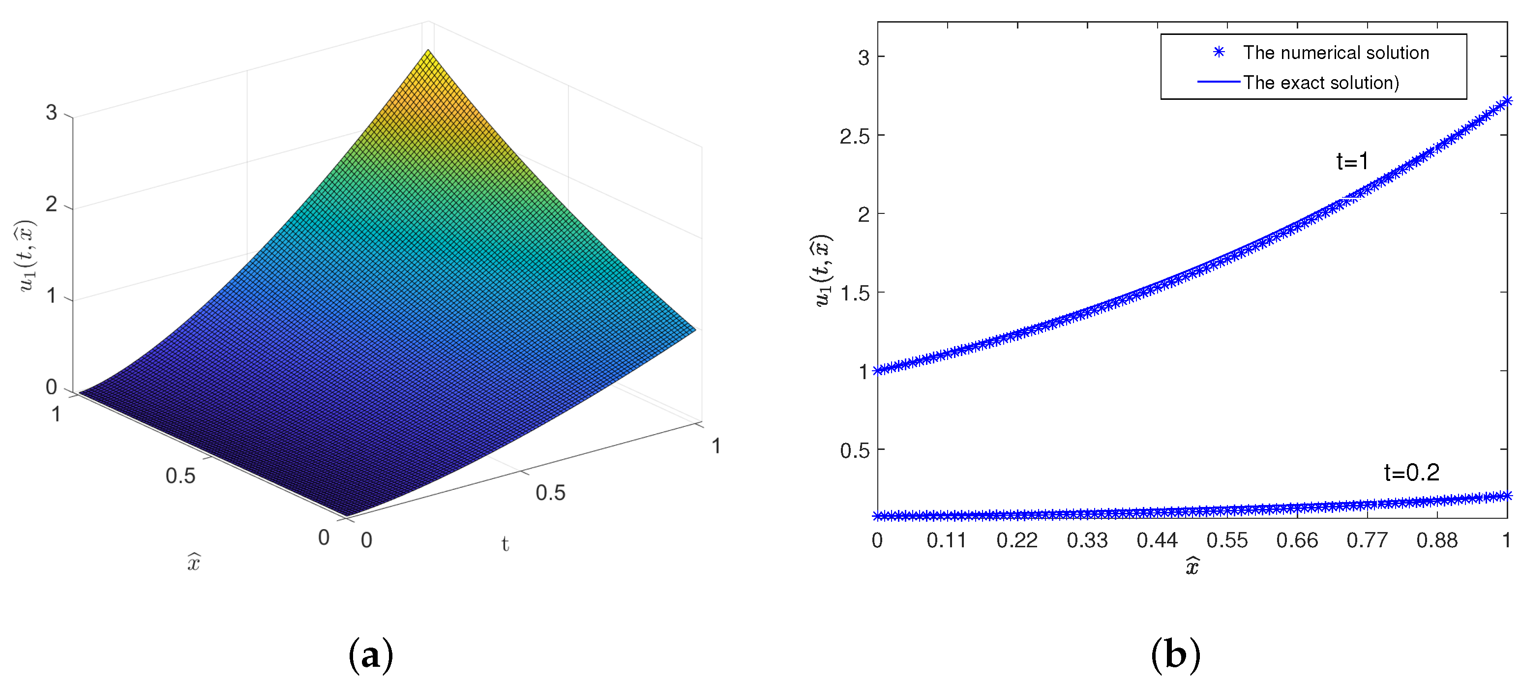
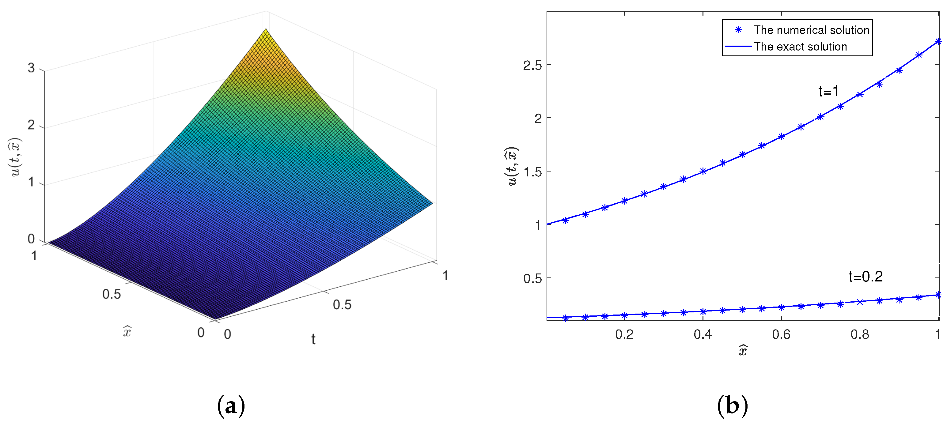
The exact solution of the system (47) is $u_1(t,\widehat{x})=e^{\widehat{x}}{t}^{1+q}$. The initial values are $u_1(0,\widehat{x})=0$, $u_1(t,0)=t^{1+q}$, and $u_1(1,t)=e{t}^{1+q}$. The nonlinearity reaction–diffusion system parameters of (47) are chosen as $q=0.5$, $a_1=0.2$, $d_1=\Gamma (2+q)$, and $b_1=-\Gamma (2+q)$, and they satisfy the conditions in Theorems 2 and 4. In addition, let $f_1(u_1(t,\widehat{x}))=u_1(t,\widehat{x})$, and $I_1(t,\widehat{x})=\Gamma (2+q)e^{\widehat{x}}t-d_1{e}^{\widehat{x}}{t}^{1+q}$. The simulation results of system (47) with $q=0.5$ and $0\le \widehat{x}\le 1,0\le t\le 1$ are given in Figure 1. When fractional order $q=0.5$, the behaviors of the solution and its derivatives of the system (47) are shown in Figure 1a.

The exact solution and numerical solution are compared in Figure 1b for $t=0.2$ and 1, respectively. Figure 1b shows that the numerical solution is in good agreement with the exact solution. Consider the exact solution $u_1(k\sigma ,\widehat{i}h)$ and numerical solution ${\tilde{u}}_1(k\sigma ,\widehat{i}h)$ obtained by the implicit difference method.

The maximum-norm error $e_{\infty }(\sigma ,h)$, temporal, and spatial convergence orders for these finite difference schemes are listed in

Table 1. Implicit difference methods of system (47).

$q=0.5,h=\frac{1}{100}$			$q=0.5,\sigma =\frac{1}{160}$
$\sigma$	$e_{\infty }(\sigma ,h)$	$T-order$	h	$e_{\infty }(\sigma ,h)$	$S-order$
${\displaystyle \frac{1}{20}}$	$5.6\times {10}^{-2}$	-	${\displaystyle \frac{1}{14}}$	$1.2\times {10}^{-2}$	-
${\displaystyle \frac{1}{40}}$	$2.7\times {10}^{-2}$	1.052	${\displaystyle \frac{1}{16}}$	$9.6\times {10}^{-3}$	1.671
${\displaystyle \frac{1}{80}}$	$1.3\times {10}^{-2}$	1.054	${\displaystyle \frac{1}{18}}$	$8.4\times {10}^{-3}$	1.340
${\displaystyle \frac{1}{160}}$	$6.4\times {10}^{-3}$	1.022	${\displaystyle \frac{1}{20}}$	$7.4\times {10}^{-3}$	1.203

. It is clear to see that the computational convergence orders are close to theoretical convergence orders; i.e., the convergence orders of the finite difference scheme Equation (18) in the temporal direction are both nearly first order and in the spatial direction are nearly second order.

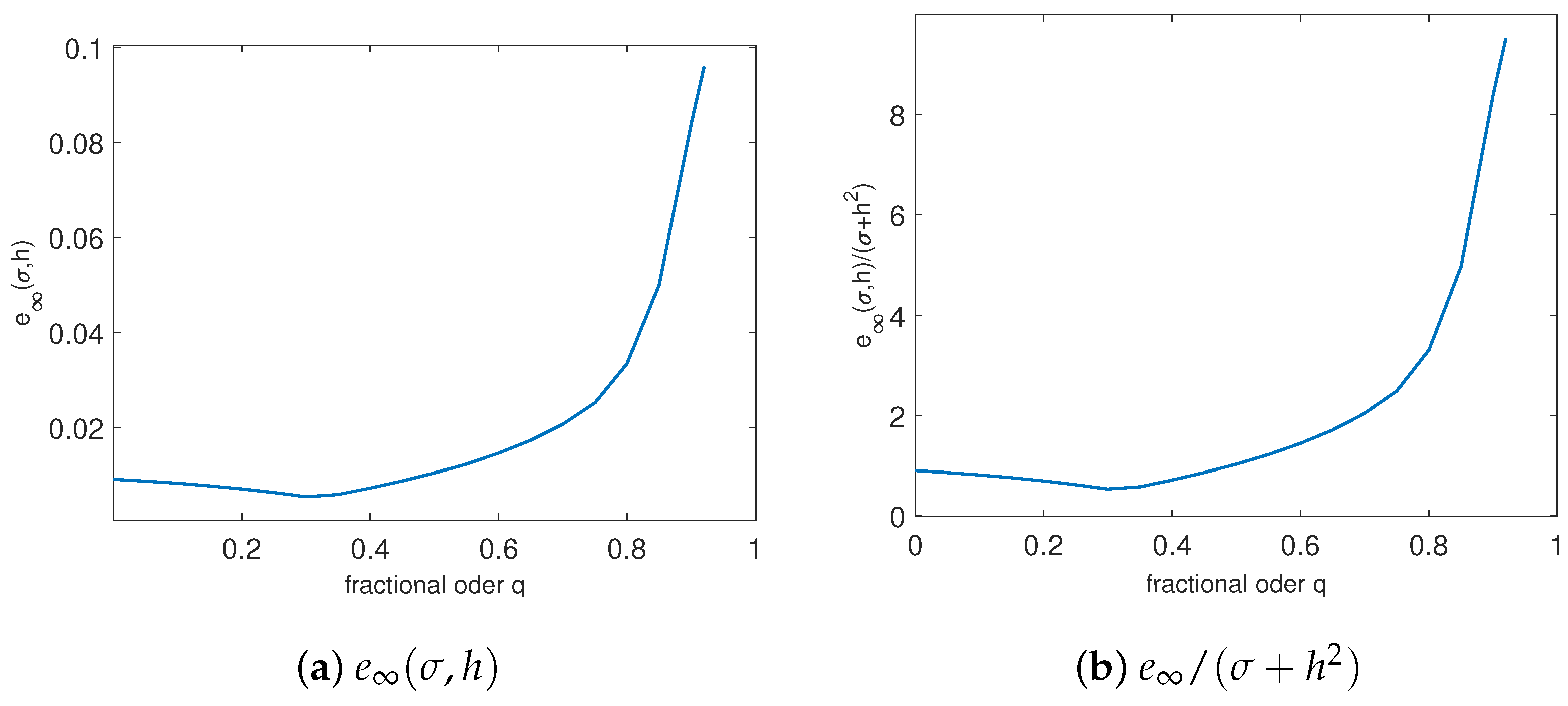
Next, we focus on the impacts of fractional-order q on the numerical solution of the equation. Choose the difference scheme as $k=\widehat{i}=100$, the fractional-order $q\in (0,1)$. $e_{\infty }(\sigma ,h)$ and $e_{\infty }(\sigma ,h)/(\sigma +h^2)$ are varying with the fractional-order q, which are given in Figure 2. From the Figure 2a, the $e_{\infty }(\sigma ,h)$ increases with the increase of q on the whole. But the increase is not very significant, as shown in Figure 2a. However, when the q increases, the $e_{\infty }(\sigma ,h)$ increases. Especially, when $0.7<q<1$, the $e_{\infty }(\sigma ,h)$ significantly increases.

According to the Riemann–Liouville fractional derivative,

$${\displaystyle \underset{q\to 1^{-}}{lim}{}_0{}^{R}D_t^{1-q}f(t,x)=\underset{q\to 1^{-}}{lim}\frac{1}{\Gamma (q)}\frac{d}{dt}{\int }_0^t\frac{f(s,x)}{{(t-s)}^{1-q}}ds,}$$

when the fractional-order $q\to 1^{-}$, differences will generate singularity, so the $e_{\infty }(\sigma ,h)$ significantly increases. Similarly, from the Figure 2b, the $e_{\infty }(\sigma ,h)/(\sigma +h^2)$ increases with the increase of q on the whole. But the increase is not very significant, as shown in Figure 2b. However, when the q increases, the $e_{\infty }(\sigma ,h)/(\sigma +h^2)$ increases. Especially, when $0.7<q<1$, the $e_{\infty }(\sigma ,h)/(\sigma +h^2)$ significantly increases.

Example 2.

A fractional-order nonlinearity ASub-DE with $n=3$ is given as follows:

$$\left\{\begin{array}{c}{\displaystyle \frac{\partial u_1(t,\widehat{x})}{\partial t}={}_0{}^{R}D_t^{1-q}\{d_1\frac{\partial u_1^2(t,\widehat{x})}{\partial {\widehat{x}}^2}+I_1(t,\widehat{x})\}-a_1{u}_1(t,\widehat{x})+\sum _{j=1}^3{b}_{1j}{f}_j(u_j(t,\widehat{x})),}\hfill \\ {\displaystyle \frac{\partial u_2(t,\widehat{x})}{\partial t}={}_0{}^{R}D_t^{1-q}\{d_2\frac{\partial u_2^2(t,\widehat{x})}{\partial {\widehat{x}}^2}+I_2(t,\widehat{x})\}-a_2{u}_2(t,\widehat{x})+\sum _{j=1}^3{b}_{2j}{f}_j(u_j(t,\widehat{x})),}\hfill \\ {\displaystyle \frac{\partial u_3(t,\widehat{x})}{\partial t}={}_0{}^{R}D_t^{1-q}\{d_3\frac{\partial u_3^2(t,\widehat{x})}{\partial {\widehat{x}}^2}+I_3(t,\widehat{x})\}-a_3{u}_3(t,\widehat{x})+\sum _{j=1}^3{b}_{3j}{f}_j(u_j(t,\widehat{x})),t>0.}\hfill \end{array}\right.$$

(48)

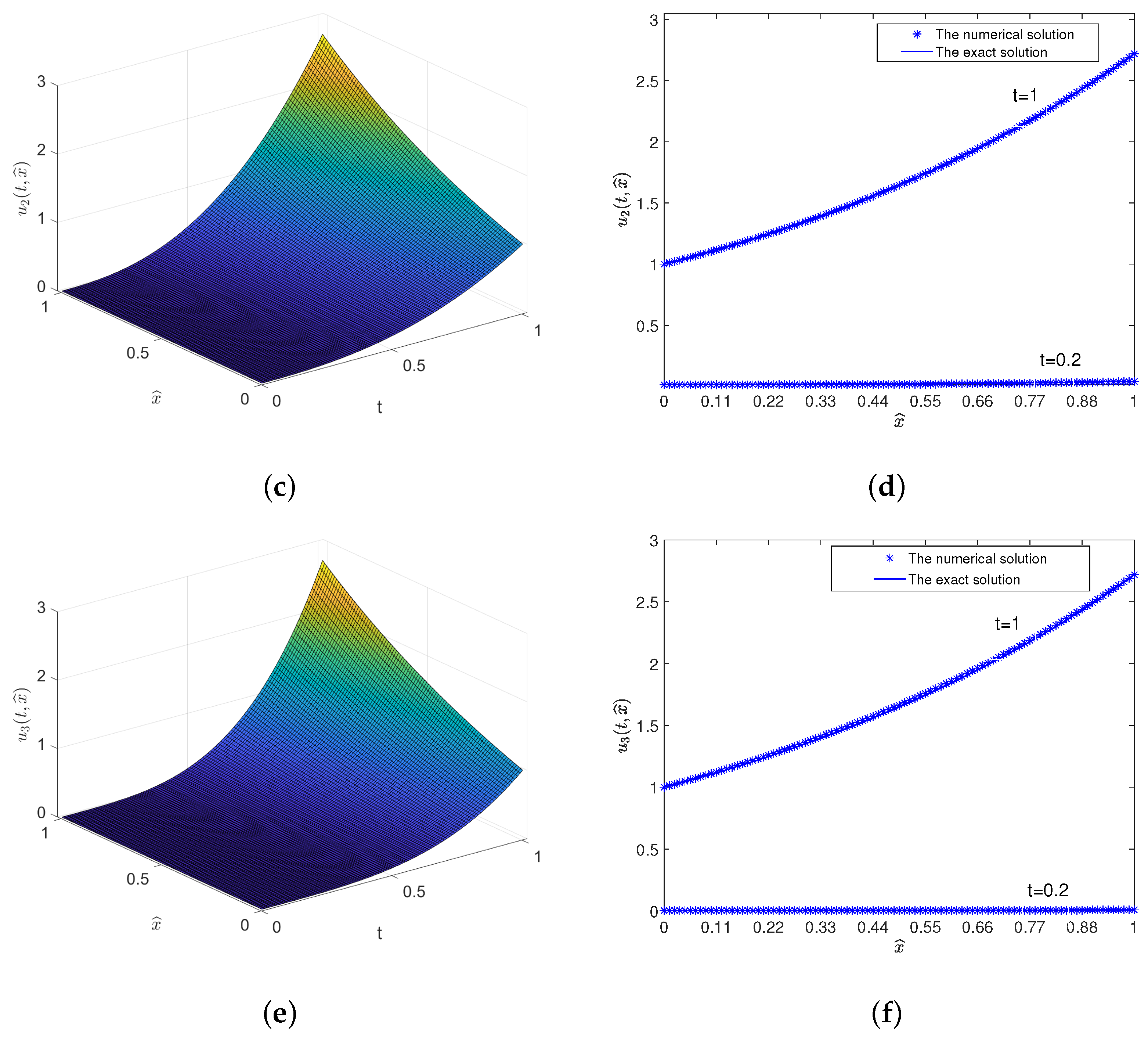
The exact solution of the system (48) is $u_1(t,\widehat{x})=e^{\widehat{x}}{t}^{1+q}$, $u_2(t,\widehat{x})=e^{\widehat{x}}{t}^{2+q}$ and $u_3(t,\widehat{x})=e^{\widehat{x}}{t}^{3+q}$. Then, the initial values $u_1(0,\widehat{x})=0$, $u_1(t,0)=t^{1+q}$, $u_1(t,1)=e{t}^{1+q}$, $u_2(0,\widehat{x})=0$, $u_2(t,0)=t^{2+q}$, $u_2(1,t)=e{t}^{1+q}$, $u_3(0,\widehat{x})=0$, $u_3(t,0)=t^{3+q}$, $u_3(1,t)=e{t}^{3+q}$. The nonlinearity reaction–diffusion system parameters of system (47) are chosen as $q=0.5$, $a_1=4.5$, $a_2=4+2q$, $a_3=3+q$, $b_{11}(t)=4.5$, $b_{22}=4+2q$, $b_{33}=3+q$, $b_{12}=2.5$, $b_{13}=0$, $b_{21}=2+q$, $b_{23}=2+q$, $b_{31}=0$, $b_{32}=3+q$, $d_1=1$, $d_2=0.3$, and $d_3=0.4$. Additionally, they satisfy the conditions in Theorems 2 and 4. We select $f_1(u_1(t,\widehat{x}))=u_1(t,\widehat{x})$, $f_2(u_2(t,\widehat{x}))=u_2(t,\widehat{x})$, and $f_3(u_3(t,\widehat{x}))=u_3(t,\widehat{x})$; then, they are continuously differentiable functions or Lipschitz continuous. We take the control input vector as $I_1(t,\widehat{x})=\Gamma (2+q)e^{\widehat{x}}t-{\displaystyle \frac{\Gamma (3+q)}{6}}{b}_{12}{e}^{\widehat{x}}{t}^3-d_1{e}^{\widehat{x}}{t}^{1+q}$, $I_2(t,\widehat{x})=-{\displaystyle \frac{\Gamma (4+q)}{\Gamma (5)}}{b}_{23}{e}^{\widehat{x}}{t}^4-d_2{e}^{\widehat{x}}{t}^{2+q}$, $I_3(t,\widehat{x})=-d_3{e}^{\widehat{x}}{t}^{3+q}$. The simulation results of system (48) with $q=0.5$, $0\le \widehat{x}\le 1,0\le t\le 1$ are shown in Figure 2. When fractional order $q=0.5$, the behaviors of the solution and its derivatives of the system (48) are shown in Figure 3 a,c,e.

The comparison results of the exact solution and numerical solution are shown in Figure 3 b,d,f, when $t=0.2$ and 1, respectively. Figure 2 shows that the numerical solutions are in good agreement with the exact solutions. We take the exact solution $u_i(k\sigma ,\widehat{i}h)(i=1,2,3)$ and numerical solution ${\tilde{u}}_i(k\sigma ,\widehat{i}h)(i=1,2,3)$ obtained by the implicit difference method.

The maximum-norm error $e_{\infty }^i(\sigma ,h)(i=1,2,3)$, temporal, and spatial convergence orders for these finite difference schemes are listed in

Table 2. Implicit difference methods of system (48).

$q=0.5,h=\frac{1}{100}$
$\sigma$	$e_{\infty }^1(\sigma ,h)$	$T-order$	$e_{\infty }^2(\sigma ,h)$	$T-order$	$e_{\infty }^3(\sigma ,h)$	$T-order$
${\displaystyle \frac{1}{20}}$	$8.02\times {10}^{-2}$	-	$4.03\times {10}^{-2}$	−	$2.4\times {10}^{-2}$	-
${\displaystyle \frac{1}{40}}$	$4.43\times {10}^{-2}$	0.856	$2.95\times {10}^{-2}$	0.451	$1.6\times {10}^{-2}$	0.532
${\displaystyle \frac{1}{80}}$	$2.07\times {10}^{-2}$	1.097	$1.36\times {10}^{-2}$	1.171	$6.3\times {10}^{-3}$	1.398
${\displaystyle \frac{1}{160}}$	$1.19\times {10}^{-2}$	1.236	$7.8\times {10}^{-3}$	0.802	$4.4\times {10}^{-3}$	0.518
$q=0.5,\sigma ={\displaystyle \frac{1}{90}}$
h	$e_{\infty }^1(\sigma ,h)$	$S-order$	$e_{\infty }^2(\sigma ,h)$	$S-order$	$e_{\infty }^3(\sigma ,h)$	$S-order$
${\displaystyle \frac{1}{52}}$	$7.60\times {10}^{-2}$	-	$6.89\times {10}^{-2}$	-	$4.12\times {10}^{-2}$	-
${\displaystyle \frac{1}{54}}$	$7.38\times {10}^{-2}$	1.683	$6.42\times {10}^{-2}$	1.872	$3.88\times {10}^{-2}$	1.815
${\displaystyle \frac{1}{56}}$	$7.17\times {10}^{-2}$	1.611	$6.01\times {10}^{-2}$	1.590	$3.65\times {10}^{-2}$	1.690
${\displaystyle \frac{1}{58}}$	$6.77\times {10}^{-2}$	1.579	$5.64\times {10}^{-2}$	1.747	$3.44\times {10}^{-2}$	1.629

. It is clear to see that the computational convergence orders are close to theoretical convergence orders; i.e., the convergence orders of the finite difference scheme Equation (18) in the temporal direction are both nearly first order and in the spatial direction are nearly second order.

Remark 10.

From the Table 2, due to the coupling effect of n-coupled nonlinearity anomalous subdiffusion systems, error components interact and cause certain deviations. It should be noted that the convergence order achieved by the proposed method is not exceptionally high; nevertheless, it establishes a implicit difference methods for solving n-coupled nonlinearity anomalous subdiffusion systems. Developing algorithms yielding more accurate numerical solutions with higher-order convergence will be focused on in future work.

5. Conclusions and Discussion

This paper presents an investigation on the numerical analysis and analytical technique of n-dimensional fractional-order nonlinearity ASub-DEs. We propose some improved implicit difference methods and discuss the stability and convergence using the improved energy methods. The stability and convergence conditions are given based on different implicit methods and related to the system dimension n. Finally, we provide two numerical examples to validate the effectiveness of our theoretical results.

There are some potential research directions that can be considered for future work. The nonlinearity term of n-dimensional fractional-order nonlinearity ASub-DEs is beyond the scope of this study. The numerical analysis of the n-dimensional fractional-order nonlinearity ASub-DEs, which have the following form, will be considered in future work:

$$\begin{array}{c}{\displaystyle \frac{\partial u_i(t,\widehat{x})}{\partial t}={}_0{}^{R}D_t^{1-q}\{d_i\frac{\partial u_i^2(t,\widehat{x})}{\partial {\widehat{x}}^2}+I_i(t,\widehat{x})-a_i{u}_i(t,\widehat{x})+\sum _{j=1}^n{b}_{ij}{f}_j(u_j(t,\widehat{x}))\},}\hfill \\ i=1,2,\dots ,n,t>0.\hfill \end{array}$$

Based on the relations between the Riemann–Liouville and Caputo definitions, we have

$$\begin{array}{c}{\displaystyle {}_0{}^{C}D_t^q{u}_i(t,\widehat{x})=d_i\frac{\partial u_i^2(t,\widehat{x})}{\partial {\widehat{x}}^2}+I_i(t,\widehat{x})-a_i{u}_i(t,\widehat{x})+\sum _{j=1}^n{b}_{ij}{f}_j(u_j(t,\widehat{x})),i=1,2,\dots ,n,t>0.}\hfill \end{array}$$

Furthermore, the maximum norm error estimate may not be sufficiently small. Therefore, constructing a high-accuracy difference scheme in the future work for solving n-dimensional fractional-order nonlinearity ASub-DEs would have both theoretical and practical significance. In addition, time delay is a well-known factor that can cause oscillations or instabilities in dynamic systems, and it can affect the stability and of the systems. Therefore, the numerical analysis of n-dimensional fractional-order nonlinearity ASub-DEs with time delay would be an interesting and challenging topic for future research.

References

1. Bouchaud, J.; Georges, A. Anomalous diffusion in disordered media: Statistical mechanisms, models and physical applications. Phys. Rep. 1990, 195, 127–293. [Google Scholar] [CrossRef]
2. Goychuk, I.; Heinsalu, E.; Patriarca, M.; Schmid, G.; Hanggi, P. Current and universal scaling in anomalous transport. Phys. Rev. E 2006, 73, 020101. [Google Scholar] [CrossRef]
3. Volpert, V.; Petrovskii, S. Reaction-diffusion waves in biology: New trends, recent developments. Phys. Life Rev. 2025, 52, 1–20. [Google Scholar] [CrossRef]
4. Oliveira, F.A.; Ferreira, R.M.S.; Lapas, L.C.; Vainstein, M.H. Anomalous diffusion: A basic mechanism for the evolution of inhomogeneous systems. Front. Phys. 2019, 19, 1–18. [Google Scholar] [CrossRef]
5. Klafter, J.; Sokolov, I.M. Anomalous diffusion spreads its wings. Phys. World 2005, 18, 29–32. [Google Scholar] [CrossRef]
6. Meroz, Y.; Sokolov, I.M. A toolbox for determining subdiffusive mechanisms. Phys. Rep. 2015, 573, 1–29. [Google Scholar] [CrossRef]
7. Höfling, F.; Franosch, T. Anomalous transport in the crowded world of biological cells. Rep. Prog. Phys. 2013, 76, 046602. [Google Scholar] [CrossRef] [PubMed]
8. Yang, J.C.; Rademacher, J.D.M. Reaction-subdiffusion systems and memory: Spectra, turing instability and decay estimates. IMA J. Appl. Math. 2021, 86, 247–293. [Google Scholar] [CrossRef]
9. Hasan, A.F.; Sergio, M.F.; Frank, J.F. Fractional Calculus and Fractional Processes with Applications to Financial Economics Theory and Application; Elsevier: Amsterdam, The Netherlands; Academic Press: Cambridge, MA, USA, 2017. [Google Scholar]
10. Podlubny, I. Fractional Differential Equations; Academic Press: San Diego, CA, USA, 1999. [Google Scholar]
11. Kilbas, A.A.; Srivastava, H.M.; Trujillo, J.J. Theory and Applications of Fractional Differential Equations; Elsevier: Amsterdam, The Netherlands, 2006. [Google Scholar]
12. Lakshmikantham, V.; Leela, S.; Devi, J.V. Theory of Fractional Dynamic Systems; Cambridge Scientific Publishers: Cambridge, MA, USA, 2009. [Google Scholar]
13. Kutner, R.; Pekalski, A.; Sznajd-Weron, K. Anomalous Diffusion, Basics to Application; Springer: Berlin/Hamburg, Germany, 1999. [Google Scholar]
14. Metzler, R.; Klafter, J. The random walk’s guide to anomalous diffusion: A fractional dynamics approach. Phys. Rep. 2000, 339, 1–77. [Google Scholar] [CrossRef]
15. Langlands, T.A.M.; Henry, B.I. The accuracy and stability of an implicit solution method for the fractional diffusion equation. J. Comput. Phys. 2005, 205, 719–736. [Google Scholar] [CrossRef]
16. Sokolov, I.M. Models of anomalous diffusion in crowded environments. Soft Matter 2012, 8, 9043. [Google Scholar] [CrossRef]
17. Zhuang, P.; Liu, F.; Anh, V.; Turner, I. Stability and convergence of an implicit numerical method for the non-linear fractional reaction-subdiffusion process. IMA J. Appl. Math. 2009, 74, 645–667. [Google Scholar] [CrossRef]
18. Zeng, F.; Li, C.; Liu, F. High-order explicit-implicit numerical methods for nonlinear anomalous diffusion equations. Eur. Phys. J.-Spec. Top. 2013, 222, 1885–1900. [Google Scholar] [CrossRef]
19. Yuste, S.B.; Acedo, L. An explicit finite difference method and a new von Neumanntype stability analysis for fractional diffusion equations. SIAM J. Numer. Anal. 2005, 42, 1862–1874. [Google Scholar] [CrossRef]
20. Yuste, S.B. Weighted average finite difference methods for fractional diffusion equations. J. Comput. Phys. 2006, 216, 264–274. [Google Scholar] [CrossRef]
21. Li, C.; Ding, H. Higher order finite difference method for the reaction and anomalousdiffusion equation. Appl. Math. Model. 2014, 38, 3802–3821. [Google Scholar] [CrossRef]
22. Jin, B.T.; Lazarov, R.; Zhou, Z. An analysis of the L1 scheme for the subdiffusion equation with nonsmooth data. IMA J. Appl. Math. 2016, 36, 197–221. [Google Scholar] [CrossRef]
23. Deng, W.H. Finite element method for the space and time fractional Fokker-Planck equation. SIAM J. Numer. Anal. 2008, 47, 204–226. [Google Scholar] [CrossRef]
24. Chen, C.M.; Liu, F.; Burrage, K. Finite difference methods and a Fourier analysis for the fractional reaction-subdiffusion equation. Appl. Math. Comput. 2007, 198, 754–769. [Google Scholar] [CrossRef]
25. Chen, C.M.; Liu, F.; Turner, I.; Anh, V. A Fourier method for the fractional diffusion equation describing sub-diffusion. J. Comput. Phys. 2007, 227, 886–897. [Google Scholar] [CrossRef]
26. Sean, D.L. Subdiffusion-limited fractional reaction-subdiffusion equations with affine reactions: Solution, stochastic paths, and applications. Phys. Rev. E 2020, 102, 042125. [Google Scholar]
27. Alexander, A.M.; Sean, D.L. Reaction-subdiffusion equations with species-dependent movement. SIAM J. Appl. Math. 2021, 81, 2457–2524. [Google Scholar] [CrossRef]
28. Cui, M. Compact finite difference method for the fractional diffusion equation. J. Comput. Phys. 2009, 228, 7792–7804. [Google Scholar] [CrossRef]
29. Gao, G.H.; Tang, R.; Yang, Q. A compact finite difference scheme for the fourth-order time multi-term fractional sub-diffusion equations with the first Dirichlet boundary conditions. INT J. Numer. Anal. Mod. 2021, 18, 100–119. [Google Scholar]
30. Zeng, F.H.; Li, C.P.; Liu, F.; Turner, I.W. Numerical algorithms for time-fractional subdiffusion equation with second-order accuracy. SIAM J. Sci. Comput. 2015, 37, 55–78. [Google Scholar] [CrossRef]
31. Chen, H.; Shi, Y.H.; Zhang, J.W.; Zhao, Y.M. Sharp error estimate of a Grunwald-Letnikov scheme for reaction-subdiffusion equations. Numer. Algorithms 2022, 89, 1465–1477. [Google Scholar] [CrossRef]
32. Dehestani, H.; Ordokhani, Y.; Razzaghi, M. A spectral approach for time-fractional diffusion and subdiffusion equations in a large interval. Math. Model. Anal. 2022, 27, 19–40. [Google Scholar] [CrossRef]
33. Hao, Z.P.; Sun, Z.Z.; Cao, W.R. A fourth-order approximation of fractional derivatives with its applications. J. Comput. Phys. 2015, 281, 787–805. [Google Scholar] [CrossRef]
34. Zhuang, P.; Liu, F.; Anh, V.; Turner, I. New solution and analytical techniques of the implicit numerical method for the anomalous subdiffusion equation. SIAM J. Numer. Anal. 2008, 46, 1079–1095. [Google Scholar] [CrossRef]
35. Liu, F.; Yang, C.; Burrage, K. Numerical method and analytical technique of the modified anomalous subdiffusion equation with a nonlinear source term. J. Comput. Appl. Math. 2008, 46, 1079–1095. [Google Scholar] [CrossRef]
36. Zhang, Y.N.; Sun, Z.Z.; Wu, H.W. Error estimates of Crank-Nicolson-Type difference schemes for the subdiffusion equation. SIAM J. Numer. Anal. 2011, 49, 2302–2322. [Google Scholar] [CrossRef]
37. Gao, G.H.; Sun, Z.Z. Two alternating direction implicit difference schemes for solving the two-dimensional time distributed-order wave equations. J. Sci. Comput. 2016, 69, 506–531. [Google Scholar] [CrossRef]
38. Roul, P.; Rohil, V. A novel high-order numerical scheme and its analysis for the two-dimensional time-fractional reaction-subdiffusion equation. Numer. Algorithms 2022, 90, 1357–1387. [Google Scholar] [CrossRef]
39. Wei, Y.B.; Zhao, Y.M.; Chen, H.; Wang, F.L.; Lu, S.J. On the convergence and superconvergence for a class of two-dimensional time fractional reaction-subdiffusion equations. Numer. Methods Partial Differ. Eq. 2023, 39, 481–500. [Google Scholar] [CrossRef]
40. Zhu, P.; Xie, S. ADI finite element method for 2D nonlinear time fractional reaction-ubdiffusion equation. Am. J. Comput. Math. 2016, 6, 336. [Google Scholar] [CrossRef]
41. Dehestani, H.; Ordokhani, Y.; Razzaghi, M. An accurate numerical scheme for three-dimensional variable-order time-fractional partial differential equations in two types of space domains. Math. Model. Anal. 2024, 29, 406–425. [Google Scholar] [CrossRef]
42. Jiang, Y.B.; Chen, H.; Huang, C.B.; Wang, J. A fully discrete GL-ADI scheme for 2D time-fractional reaction-subdiffusion equation. Appl. Math. Comput. 2025, 488, 129147. [Google Scholar] [CrossRef]
43. Jiang, Y.B.; Chen, H. Local convergence analysis of L1-ADI scheme for two-dimensional reaction-subdiffusion equation. J. Comput. Appl. Math. 2024, 70, 1953–1964. [Google Scholar] [CrossRef]
44. Kumari, T.; Roul, P. An efficient computational technique for solving a time-fractional reaction-subdiffusion model in 2D space. Comput. Math. Appl. 2024, 160, 191–208. [Google Scholar] [CrossRef]
45. Roul, P.; Yadav, J.; Kumari, T. An efficient computational approach and its analysis for the Caputo time-fractional convection reaction-diffusion equation in two-dimensional space. Math. Method. Appl. Sci. 2025, 48, 155–175. [Google Scholar] [CrossRef]
46. Yuste, S.; Acedo, L.; Lindenberg, K. Reaction front in an A + BC reaction-subdiffusion process. Phys. Rev. E 2004, 69, 036126. [Google Scholar] [CrossRef] [PubMed]
47. Seki, K.; Wojcik, M.; Tachiya, M. Fractional reaction-diffusion equation. J. Chem. Phys. 2003, 119, 2165–2170. [Google Scholar] [CrossRef]
48. Li, C.P.; Deng, W.H. Remarks on fractional derivatives. Appl. Math. Comput. 2007, 187, 777–784. [Google Scholar] [CrossRef]
49. Ding, H.; Li, C.P. High-order compact difference schemes for the modified anomalous subdiffusion equation. Numer. Methods Part 2016, 32, 213–242. [Google Scholar] [CrossRef]
Figure 1. Numerical solution of the system (47), when q = 0.5 . (a) Numerical solution. (b) Numerical solution and exact solution when t = 0.2 , 1 .
Fractalfract 09 00420 g001
Figure 2. Numerical solution of the system (47) about fractional order q.
Fractalfract 09 00420 g002
Figure 3. Numerical solution of the system (48), when q = 0.5 . (a) Numerical solution of u 1 ( t , x ^ ) . (b) Exact solution and of numerical solution u 1 ( t , x ^ ) when t = 0.2 , 1 . (c) Numerical solution of u 2 ( t , x ^ ) . (d) Exact solution and of numerical solution of u 2 ( t , x ^ ) when t = 0.2 , 1 . (e) Numerical solution of u 3 ( t , x ^ ) . (f) Exact solution and of numerical solution of u 3 ( t , x ^ ) when t = 0.2 , 1 .
Fractalfract 09 00420 g003aFractalfract 09 00420 g003b