Averaged Systems of Stochastic Differential Equations with Lévy Noise and Fractional Brownian Motion

Abstract

In some problems, partial differential equations are reduced to ordinary differential equations. In special cases, when incorporating randomness, equations can be reduced to systems of stochastic differential Equations (SDEs). Stochastic averaging for a class of stochastic differential equations with fractional Brownian motion and non-Gaussian Lévy noise is considered. Stability criteria for systems of stochastic differential equations with fractional Brownian motion and non-Gaussian Lévy noise do not currently exist. Usually, studies on determining the sensitivity of solutions to the accuracy of setting the initial conditions are being conducted to explain the phenomenon of deterministic chaos. These studies show both convergence in mean square and convergence in probability to averaged systems of stochastic differential equations driven by fractional Brownian motion and Lévy process. The solutions to systems can be approximated by solutions to averaged stochastic differential equations by using the stochastic averaging.

1. Introduction

In the 1940s, Japanese mathematician K. Ito laid the foundations of the theory of stochastic differential equations. Initially, such equations were used to describe diffusion processes in the language of probability theory. Later, it turned out that stochastic equations are a convenient tool for solving many applied problems. Stochastic models are used to study various physical, chemical, and sociological processes that are characterized by random deviations (various errors, noise, and instability of factors influencing the process).

Lévy noise (or Lévy processes) generalizes Brownian motion by allowing jumps (discontinuous paths), heavy tails (more extreme events), and skewness (asymmetry in distributions). Stochastic differential equations with Lévy noise extend standard SDEs driven by Brownian motion by incorporating jumps, modeling more complex and realistic random behavior, especially in finance, biology, and engineering systems; see [1,2,3].

The noise from a Lévy process is obtained by decomposing it by Levy–Itô into Brownian motion (continuous case) and an independent Poisson random metric (jumping case); it has attracted particular attention in recent years. It should be noted that Poisson noise is a special non-Gaussian Lévy noise.

As an essential class of stochastic processes, the Lévy process is a rich mathematical object with potential applications in many areas. Recently, a martingale representation theory related to a class of Lévy processes was introduced by [1].

Stochastic averaging is a mathematical technique used to simplify the analysis of stochastic differential equations, especially when the system exhibits slow and fast dynamics (variables that evolve on different time scales). The core idea is to average out the effects of fast-changing (often noisy) components to study the behavior of the slower dynamics more effectively; see [4,5,6,7]. If we have a slow system with $x\left(t\right)$ and fast stochastic process $y\left(t\right)$, let $ϵ<1$ indicate that $y\left(t\right)$ evolves much faster than $x\left(t\right)$ and consider a dynamics described by

$$\left\{\begin{array}{cc}dx=f(U,V)dt\hfill & \\ dy={\displaystyle \frac{1}{ϵ}}g(U,V)dt+{\displaystyle \frac{1}{\sqrt{ϵ}}}h(U,V)d{w}_t,\hfill \end{array}\right.$$

here, $w_t$ is a Wiener process (It will be considered Brownian motion in our paper).

As $ϵ\to 0$ the fast process $y\left(t\right)$ reaches a stationary distribution quickly. Stochastic averaging replaces the influence of y on x with its average effect over this distribution. Then, the reduced (averaged) system becomes as follows:

$$dx=F\left(x\right)dt$$

where

$$F\left(x\right)=\int f(U,V){\mu }_x\left(dy\right),$$

and ${\mu }_x\left(dy\right)$ is the invariant measure of the fast process $y\left(t\right)$ given x is fixed.

To date, a considerable number of theories and techniques have been introduced for exploring stochastic systems, the most important of which relates to approximation theory, through which a simplified system is introduced to replace the original system to require a certain relationship between their solutions; see [8,9,10].

In relation to the motivation for our paper, we should mention the work by [11], where a fractional white noise calculus is developed and used to markets modeled by (Wick–) Itô type of stochastic differential equations defined by fractional Brownian motion in the case $1/2<H<1$; see [2,12].

Regarding the averaged principle of stochastic differential equations with fractional Brownian motion, one can review the related results in [13]. The authors establish an averaging principle for SDEs with fBm and demonstrate that the solutions to the averaged equations converge to those of the original equations in mean square and probability.

The averaging principle for Caputo-type fractional stochastic differential equations with Lévy noise is considered in [14], and sufficient conditions for the averaging principle of Caputo-type FSDEs with Lévy noise are provided, addressing singular integral kernels caused by fractional integration and proving the desired averaging principle; see [15]. In the first part of the paper, the main background tools used in the proof are considered in Section 2, such as stochastic calculus and their properties related to fractional Brownian motion. In Section 3, we state and prove our main result, showing the stochastic averaging principle for stochastic differential equations with fractional Brownian motion and non-Gaussian Lévy noise. Finally, two illustrated examples are given applying the stochastic averaging principle.

2. Background Tools

To define and work with stochastic processes, let us introduce the space $\left(\Omega ,\mathcal{F},\mathbb{P}\right)$, which is the usual complete probability space, and let ${\left({\mathcal{F}}_t\right)}_{t\ge 0}$ be a filtration such that ${(\mathcal{F}={\mathcal{F}}_t)}_{t\ge 0}$ satisfies

• Right continuous: ${\mathcal{F}}_t={\cap }_{s>t}{\mathcal{F}}_s$.
• The completeness: Each ${\mathcal{F}}_t$ contains all $\mathbb{P}$-null sets in $\mathcal{F}$).

Then, the tuple $\left(\Omega ,\mathcal{F},{\mathcal{F}}_t{)}_{t\ge 0},\mathbb{P}\right)$ is called a filtered probability space. This framework is necessary to define the stochastic process $x(·,·):[0,T]\times \Omega \to {\mathbb{R}}^n$, which will be written, for simplicity, as $x\left(t\right)$; see [16,17,18].

Definition 1.

(Lévy process) Let $L\left(t\right)$ be a stochastic process given on $\left(\Omega ,\mathcal{F},\mathbb{P}\right)$. It is said that $L\left(t\right)$ is a Lévy process if

(i) 

$L\left(0\right)=0(a.s).$

(ii) 

$L\left(t\right)$ has independent and stationary increments.

(iii) 

$L\left(t\right)$ is stochastically continuous

$$\underset{t\to s}{lim}P(\mid L\left(t\right)-L\left(s\right)\mid >a)=0,\forall a>0;\forall s\ge 0.$$

This is equivalent to

$$\underset{t\to 0}{lim}P(\mid L\left(t\right)\mid >a)=0.$$

The Lévy process is characterized by a drift coefficient $p\in {\mathbb{R}}^d$, a covariance $d\times d$ matrix A, and a nonnegative Borel measure ν defined on $({\mathbb{R}}^d,\mathcal{B}\left({\mathbb{R}}^d\right))$ and concentrated on ${\mathbb{R}}^d-\left\{0\right\}$. Then, for $\eta \in \mathcal{B}({\mathbb{R}}^d-\left\{0\right\})$, here 0 is not in the closure of η, where

$${\int }_{{\mathbb{R}}^d-\left\{0\right\}}{\left(\right|x|}^2\wedge 1)\nu \left(dx\right)<\infty .$$

or

$${\int }_{{\mathbb{R}}^d-\left\{0\right\}}{\displaystyle \frac{x^2}{x^2+1}}\nu \left(dx\right)<\infty .$$

This ν is the so-called Lévy jump metric of the Lévy process $L\left(t\right)$.

Theorem 1

([10]). (Lévy–Itô decomposition) Let $L_l\left(t\right)$ be a Lévy process. Then $\exists b_1\in {\mathbb{R}}^d$, a Brownian motion $W_l$ for each $l=1,2$ and an independent Poisson random measure N on ${\mathbb{R}}^{+}\times ({\mathbb{R}}^d-\left\{0\right\})$, where

$$L_l\left(t\right)=b_{1}t+W_l\left(t\right)+{\int }_{\left|x\right|\ge c}xN(t,dx)+{\int }_{\left|x\right|<c}x\tilde{N}(t,dx),t\ge 0,$$

(1)

here $N(dt,dx)$ is a Poisson random measure, and $\tilde{N}(t,dx)=N(t,dx)-t\nu \left(dx\right)$ is the compensated Poisson random measure for $L_l\left(t\right)$ and

$$b_1=E\left(L\left(1\right)\right)-{\int }_{\left|x\right|\ge c}xN(1,dx),$$

where $c\in {\mathbb{R}}^{+}\cup \{+\infty \}$.

2.1. Fractional Brownian Motion and Long-Range Dependence

Fractional Brownian motion is a generalization of classical Brownian motion that introduces memory into the process. It was introduced by Benoît Mandelbrot and John van Ness in 1968.

Definition 2.

Let $H\in (0,1)$ be the Hurst parameter. The fractional Brownian motion $B^H={\left(B_t^H\right)}_{t\ge 0}$ with Hurst index H is a centered self-similar Gaussian process with

(i) 

$B^H\left(0\right)=0.$

(ii) 

Zero mean:

$$E\left(B_t^H\right)=0,t\in {\mathbb{R}}^{+}.$$

(iii) 

Covariance function:

$$E\left(B_t^H{B}_s^H\right)={\displaystyle \frac{1}{2}}{\left(\right|t|}^{2H}+{\left|s\right|}^{2H}{+|t-s|}^{2H}),t,s\in {\mathbb{R}}^{+}.$$

Remark 1.

1.

When $H={\displaystyle \frac{1}{2}},$ fractional Brownian motion reduces to standard Brownian motion.

2.

Given that the fractional Brownian motion is not a semi-martingale unless $H={\displaystyle \frac{1}{2}}$, Itô calculus does not apply directly.

3.

Self-similarity:

$$B_{ct}^H=c^H{B}_t^H,t\ge 0,c>0.$$

4.

Stationary increments:

$$B_{t+s}^H-B_s^H\equiv B_t^{H}t,s\ge 0.$$

5.

Long-range dependence:

(a) 

If $H>{\displaystyle \frac{1}{2}}$: Positive correlation (persistence), it can be applied in Riemann–Stieltjes integrals.

(b) 

If $H<{\displaystyle \frac{1}{2}}$: Negative correlation (anti-persistence), it can be applied in Rough path theory, especially when $H\in ({\displaystyle \frac{1}{4}},{\displaystyle \frac{1}{2}})$.

Let $f\in C({\mathbb{R}}^{+},{\mathbb{R}}^{+})$ be Borel measurable and ${\displaystyle \frac{1}{2}}\le H<1$. $\varpi \in C({\mathbb{R}}^{+}\times {\mathbb{R}}^{+},{\mathbb{R}}^{+})$ be defined as

$$\varpi (t,s)={H(2H-1)|t-s|}^{2H-2},t,s\in {\mathbb{R}}^{+},$$

So, we have

$$L_{\varpi }^2={\{f:|f|}_{\varpi }^2={\int }_{{\mathbb{R}}^{+}}{\int }_{{\mathbb{R}}^{+}}f\left(t\right)f\left(r\right)\varpi (t,r)drdt<\infty \}.$$

equipped with the following inner product

$${\langle f_1,f_2\rangle }_{\varpi }={\int }_{{\mathbb{R}}^{+}}{\int }_{{\mathbb{R}}^{+}}{f}_1\left(t\right)f_2\left(r\right)\varpi (t,r)drdt$$

then $L_{\varpi }^2\left({\mathbb{R}}^{+}\right)$ will be a separable Hilbert space.

Let us now define $\mathcal{S}$ as a set of smooth and cylindrical random variables as

$$F=f(B^H\left({\psi }_1\right),B^H\left({\psi }_2\right),\dots ,B^H\left({\psi }_n\right)),n\ge 1,$$

here $f\in C_b^{\infty }\left({\mathbb{R}}^n\right)$, ${\psi }_i\in \mathcal{H}$, $\mathcal{H}$ is a Hilbert space; for more detail, please see [19,20].

The derivative operator $D_t^H$ of a F is given as the $\mathcal{H}$-valued random variable as follows:

$$D_t^{H}F=\sum _{i=1}^n{\displaystyle \frac{\partial f}{\partial x_i}}(B^H\left({\psi }_1\right),B^H\left({\psi }_2\right),\dots ,B^H\left({\psi }_n\right)){\psi }_i.$$

As in [21], the Malliavin $\varpi$-derivative of F is given as

$$D_t^{\varpi }F={\int }_{{\mathbb{R}}^{+}}\varpi (t,r)D_r^{H}Fdr.$$

Definition 3.

Let $y\left(t\right)$ be a stochastic process with integrable trajectories.

(1) 

The symmetric integral of $y\left(t\right)$ with respect to $B^H\left(t\right)$ is given as the limit in the probability as $\tau \to 0$ for

$${\displaystyle \frac{1}{2\tau }}{\int }_0^{T}y\left(r\right)\left(B^H(r+\tau )-B^H(r-\tau )\right)dr,$$

provided that this limit is present in the probability given by

$${\int }_0^{T}y\left(r\right)d^{\circ }{B}^H\left(r\right).$$

(2) 

The forward integral of $y\left(t\right)$ with respect to $B^H$ is defined as the limit in the probability when $\tau \to 0$ of

$${\displaystyle \frac{1}{\tau }}{\int }_0^{T}y\left(r\right)\left({\displaystyle \frac{B^H(r+\tau )-B^H\left(r\right)}{\tau }}\right)dr,$$

provided that this limit is present in the probability given by

$${\int }_0^{T}y\left(r\right)d^{-}{B}^H\left(r\right).$$

(3) 

The backward integral of $y\left(t\right)$ with respect to $B^H$ is defined as the limit in probability as $\tau \to 0$ of

$${\displaystyle \frac{1}{\tau }}{\int }_0^{T}y\left(r\right)\left({\displaystyle \frac{B^H(r-\tau )-B^H\left(r\right)}{\tau }}\right)dr,$$

provided that this limit is present in the probability given by

$${\int }_0^{T}y\left(r\right)d^{+}{B}^H\left(r\right).$$

Remark 2

([21]). Let ${\mathcal{L}}_{\varpi }(0,T)$ of integrands be defined as the family of stochastic processes $y\left(t\right)$ on $[0,T]$ such that $y\left(t\right)\in {\mathcal{L}}_{\varpi }(0,T)$ if ${E\left|y\left(t\right)\right|}_{\varpi }^2<\infty$. Assume that $y\left(t\right)$ is a stochastic process in $L(0,T)$ and satisfies

$${\int }_0^T{\int }_0^T|D_r^H{y\left(t\right)||t-r|}^{2H-2}drdt<\infty .$$

Then there is the symmetric integral, and the following relationship is true:

$${\int }_0^{T}y\left(r\right)d^{\circ }{B}^H\left(r\right)={\int }_0^{T}y\left(r\right)\diamond d{B}^H\left(r\right)+{\int }_0^T\left(D_r^{\varpi }y\left(t\right)\right)dr,$$

(2)

here, ⋄ represents the Wick product, ${\displaystyle \frac{1}{2}}<H<1$.

Remark 3

([21]). Let $y\left(t\right)\in {\mathcal{L}}_{\varpi }(0,T)$. We define the forward and backward integrals with respect to fractional Brownian motion as follows:

$${\int }_0^{T}y\left(r\right)d^{-}{B}^H\left(r\right)={\int }_0^{T}y\left(r\right)\diamond d{B}^H\left(r\right)+{\int }_0^T\left(D_r^{\varpi }y\left(t\right)\right)dr$$

(3)

and

$${\int }_0^{T}y\left(r\right)d^{+}{B}^H\left(r\right)={\int }_0^{T}y\left(r\right)\diamond d{B}^H\left(r\right)+{\int }_0^T\left(D_r^{\varpi }y\left(t\right)\right)dr$$

(4)

To introduce the principle of random means (averaging), we need the lemma.

Lemma 1

([22]). Let $\vartheta \left(s\right)$ be a stochastic process in ${\mathcal{L}}_{\varpi }(0,T)$ and $B^H\left(t\right)(H>{\displaystyle \frac{1}{2}}$) be a fractional Brownian motion. Then, $\forall T\in (0,\infty )$, $\exists C(H,T)$ a constant such that the following inequality holds

$${\int }_0^T{\left(\vartheta \left(s\right)d^{\circ }{B}^H\left(s\right)\right)}^2\le 2C(H,T)E(\left({\int }_0^T{\left|\vartheta \left(s\right)\right|}^{2}ds\right)+4C{T}^2$$

(5)

where $C(H,T)=H{T}^{2H-1}.$

The Lévy–Itô decomposition is a fundamental result in the theory of Lévy processes, which generalizes Brownian motion and Poisson processes.

Theorem 2.

(Lévy–Itô Decomposition Theorem) Let $X_t$ be a Lévy process in ${\mathbb{R}}^d$. Then it can be uniquely decomposed as follows:

$$X_t=bt+\sigma W_t+{\int }_{\left|x\right|\ge 1}xN(t,dx)+{\int }_{\left|x\right|\ge 1}x\tilde{N}(t,dx),$$

where the following holds:

1.

$b\in {\mathbb{R}}^d$ is the drift vector.

2.

$\sigma W_t$ represents Brownian motion part (with diffusion coefficient σ).

3.

$N(t,dx)$ is the Poisson random measure counting jumps of size x.

4.

$\tilde{N}(t,dx)=N(t,dx)-\nu \left(dx\right)dt$ is the compensated Poisson random measure.

5.

$\nu \left(dx\right)$ is the Lévy measure, satisfying

$${\int }_{{\mathbb{R}}^d/\left\{0\right\}}{(1\wedge |x|}^2)\nu \left(dx\right)<\infty .$$

2.2. Fractional Brownian Motion and Lévy Process for Stochastic Differential Equations

We discuss the symmetric integration of stochastic differential equations with respect to fractional Brownian motion and Lévy process. We consider nonlinear stochastic differential equations driven by fractional Brownian motion and Lévy process on ${\mathbb{R}}^d$ as follows:

$$\left\{\begin{array}{cc}dU\left(t\right)\hfill & =f^1(t,U\left(t-\right),V\left(t-\right))dt+{\sigma }^1(t,U\left(t-\right)),V\left(t-\right))d{L}_1\left(t\right)\hfill \\ \\ \hfill & +A^1(t,U\left(t-\right),V\left(t-\right))d^{\circ }{B}^{H_1}\left(t\right),t\in [0,T]\hfill \\ \\ dV\left(t\right)\hfill & =f^2(t,U\left(t-\right),V\left(t-\right))dt+{\sigma }^2(t,U\left(t-\right)),V\left(t-\right))d{L}_2\left(t\right)\hfill \\ \\ \hfill & +A^2(t,U\left(t-\right),V\left(t-\right))d^{\circ }{B}^{H_2}\left(t\right),t\in [0,T]\hfill \\ \\ U\left(0\right)\hfill & =u_0,\hfill \\ \\ V\left(0\right)\hfill & =v_0,\hfill \end{array}\right.$$

(6)

with given initial value $u_0,v_0$. Here we assume that the mappings

$$f_i^1,f_i^2:[0,T]\times {\mathbb{R}}^d\times {\mathbb{R}}^d\to \mathbb{R},$$

$${\sigma }^1,{\sigma }^2:[0,T]\times {\mathbb{R}}^d\times {\mathbb{R}}^d\to \mathbb{R},$$

and

$$A^1,A^2:[0,T]\times {\mathbb{R}}^d\times {\mathbb{R}}^d\to \mathbb{R},$$

are measurable, $L\left(t\right)$ is a Lévy process, and the processes $B^H\left(t\right)$ represent d-dimensional fractional Brownian motions with Hurst parameter $H_1,H_2\in ({\displaystyle \frac{1}{2}},1)$.

Owing to the Lévy–Itô decomposition (1) into (6), we can rewrite this as follows

$$\left\{\begin{array}{cc}dU\left(t\right)\hfill & =f_1^1(t,U\left(t-\right),V\left(t-\right))dt+{\sigma }^1(t,U\left(t-\right)),V\left(t-\right))d{W}_1\left(t\right)\hfill \\ \hfill & +A^1(t,U\left(t-\right),V\left(t-\right))d^{\circ }{B}^{H_1}\left(t\right)\hfill \\ \hfill & +{\int }_{\left|x\right|\ge c}{\sigma }^1(t,U\left(t-\right),V\left(t-\right))xN(dt,dx)\hfill \\ \hfill & +{\int }_{\left|x\right|<c}{\sigma }^1(t,U\left(t-\right),V\left(t-\right)x)\tilde{N}(dt,dx),t\in [0,T]\hfill \\ \\ dV\left(t\right)\hfill & =f_2^2(t,U\left(t-\right),V\left(t-\right))dt+{\sigma }^2(t,U\left(t-\right)),V\left(t-\right))d{W}_2\left(t\right)\hfill \\ \hfill & +A^2(t,U\left(t-\right),V\left(t-\right))d^{\circ }{B}^{H_2}\left(t\right)\hfill \\ \hfill & +{\int }_{\left|x\right|\ge c}{\sigma }^2(t,U\left(t-\right),V\left(t-\right))xN(dt,dx)\hfill \\ \hfill & +{\int }_{\left|x\right|<c}{\sigma }^2(dt,U\left(t-\right),V\left(t-\right)x)\tilde{N}(t,dx),t\in [0,T]\hfill \\ U\left(0\right)\hfill & =u_0,\hfill \\ V\left(0\right)\hfill & =v_0,\hfill \end{array}\right.$$

(7)

where $f_1^1=b_1{\sigma }^1+f^1$ and $f_2^2=b_1{\sigma }^2+f^2$.

The more general form of (7) can be rewritten as follows:

$$\left\{\begin{array}{cc}dU\left(t\right)\hfill & =b^1(t,U\left(t-\right),V\left(t-\right))dt+g^1(t,U\left(t-\right)),V\left(t-\right))d{W}_1\left(t\right)\hfill \\ \hfill & +A^1(t,U\left(t-\right),V\left(t-\right))d^{\circ }{B}^{H_1}\left(t\right)\hfill \\ \hfill & +{\int }_{\left|x\right|\ge c}{F}^1(t,U\left(t-\right),V\left(t-\right),x)N(dt,dx)\hfill \\ \hfill & +{\int }_{\left|x\right|<c}{G}^1(dt,U\left(t-\right),V\left(t-\right),x)\tilde{N}(dt,dx),t\in [0,T]\hfill \\ \\ dV\left(t\right)\hfill & =b^2(t,U\left(t-\right),V\left(t-\right))dt+g^2(t,U\left(t-\right)),V\left(t-\right))d{W}_2\left(t\right)\hfill \\ \hfill & +A^2(t,U\left(t-\right),V\left(t-\right))d^{\circ }{B}^{H_2}\left(t\right)\hfill \\ \hfill & +{\int }_{\left|x\right|\ge c}{F}^2(t,U\left(t-\right),V\left(t-\right),x)N(dt,dx)\hfill \\ \hfill & +{\int }_{\left|x\right|<c}{G}^2(dt,U\left(t-\right),V\left(t-\right),x)\tilde{N}(dt,dx),t\in [0,T]\hfill \\ U\left(0\right)\hfill & =u_0,\hfill \\ V\left(0\right)\hfill & =v_0,\hfill \end{array}\right.$$

(8)

In the right-hand side of (8), we have (8)₃ representing small jumps and (8)₄ representing large jumps involving G (or F, respectively) being absent when we take $c=\infty$. Then, terms (8) involving large jumps are controlled by $F^l$ for each $l=1,2$, which can be neglected using the entanglement technique [2]. It makes sense to start by eliminating this term and focusing on studying the equation resulting from continuous noise interspersed with small jumps. For this, we present modified related SDEs

$$\left\{\begin{array}{cc}dU\left(t\right)\hfill & =b^1(t,U\left(t-\right),V\left(t-\right))dt+g^1(t,U\left(t-\right)),V\left(t-\right))d{W}_1\left(t\right)\hfill \\ \hfill & +A^1(t,U\left(t-\right),V\left(t-\right))d^{\circ }{B}^{H_1}\left(t\right)\hfill \\ \hfill & +{\int }_{\left|x\right|<c}{G}^1(t,U\left(t-\right),V\left(t-\right),x)\tilde{N}(dt,dx),t\in [0,T]\hfill \\ \\ dV\left(t\right)\hfill & =b^2(t,U\left(t-\right),V\left(t-\right))dt+g^2(t,U\left(t-\right)),V\left(t-\right))d{W}_2\left(t\right)\hfill \\ \hfill & +A^2(t,U\left(t-\right),V\left(t-\right))d^{\circ }{B}^{H_2}\left(t\right)\hfill \\ \hfill & +{\int }_{\left|x\right|<c}{G}^2(t,U\left(t-\right),V\left(t-\right),x)\tilde{N}(dt,dx),t\in [0,T]\hfill \\ U\left(0\right)\hfill & =u_0,\hfill \\ V\left(0\right)\hfill & =v_0,\hfill \end{array}\right.$$

(9)

Here, we assume that the mappings $b_i^1,b_i^2:[0,T]\times {\mathbb{R}}^d\times {\mathbb{R}}^d\to \mathbb{R}$ and $g_{ij}^1,g_{ij}^2:[0,T]\times {\mathbb{R}}^d\times {\mathbb{R}}^d\to \mathbb{R}$, $G_i^1,G_i^2:[0,T]\times {\mathbb{R}}^d\times {\mathbb{R}}^d\times {\mathbb{R}}^d\to \mathbb{R}$ to be measurable for $W_l\left(t\right)$ represents d-dimensional Brownian motion, $\tilde{N}(dt,dx)$ is the compensated Poisson random measure for $L_l\left(t\right)$ for each $l=1,2$, and we suppose that

$$P\left({\int }_0^t{\int }_{\left|x\right|<c}{\left|G^1(r,U\left(r-\right)V\left(r-\right),x)\right|}^2\nu \left(dx\right)dr<\infty \right)=1,$$

is satisfied. Very recently, for one system and $A^l\equiv 0$, problem (9) was studied by Yong Xu et al. [23]. In [13], the authors present the stochastic averaging principle for dynamical systems.

To introduce a solution for (9), we give the next space of continuous functions denoted by ${\mathcal{M}}^2$, which is the space of all functions $U(t,w):\Omega \times [0,T]⟶{\mathbb{R}}^d$ that are measurable in w for each fixed $t\in [0,T]$ and are right continuous with left limits in t for $a,e.$ and fixed $w\in \Omega ,$ endowed with the norm

$${\parallel x\parallel }_{{\mathcal{M}}^2}=E(\underset{t\in [0,T]}{sup}{\parallel U(t,.)\parallel }^2{)}^{{\displaystyle \frac{1}{2}}},$$

Lemma 2

([24]). ${\mathcal{M}}^2$ equipped with ${\parallel ·\parallel }_{{\mathcal{M}}^2}$ is a Banach space

Definition 4.

We say that an ${\mathbb{R}}^d-$ valued stochastic process is right continuous with left limit process $y=(U,V)\in {\mathcal{M}}^2\times {\mathcal{M}}^2$ being a solution to (9) in the space $\left(\Omega ,\mathcal{F},\mathbb{P}\right)$, if the following holds:

(1) 

$y\left(t\right)$ is ${\mathcal{F}}_t$-adapted $\forall t\in J=[0,T]$.

(2) 

$y\left(t\right)$ satisfies that for $t\in J$, a.e. $w\in \Omega$,

$$\left\{\begin{array}{cc}U\left(t\right)\hfill & =u_0+{\int }_0^t{b}^1(s,U\left(s-\right),V\left(s-\right))ds\hfill \\ \hfill & +{\int }_0^t{g}^1(s,U\left(s-\right)),V\left(s-\right))d{W}_1\left(s\right)\hfill \\ \hfill & +{\int }_0^t{A}^1(s,U\left(s-\right),V\left(s-\right))d^{\circ }{B}^{H_1}\left(s\right)\hfill \\ \hfill & +{\int }_0^t{\int }_{\left|x\right|<c}{G}^1(s,U\left(s-\right),V\left(s-\right),x)\tilde{N}(ds,dx),s\in [0,T]\hfill \\ V\left(t\right)\hfill & =v_0+{\int }_0^t{b}^2(s,U\left(s-\right),V\left(s-\right))ds\hfill \\ \hfill & +{\int }_0^t{g}^2(s,U\left(s-\right)),V\left(s-\right))d{W}_2\left(s\right)\hfill \\ \hfill & +{\int }_0^t{A}^2(s,U\left(s-\right),V\left(s-\right))d^{\circ }{B}^{H_2}\left(s\right)\hfill \\ \hfill & +{\int }_0^t{\int }_{\left|x\right|<c}{G}^2(s,U\left(s-\right),V\left(s-\right),x)\tilde{N}(ds,dx),t\in [0,T]\hfill \end{array}\right.$$

(10)

The following result is known as Gronwall–Bihari’s Theorem.

Lemma 3

([20]). Let $y,g:J\to \mathbb{R}$ be positive real continuous functions. Assume that $\exists c>0$ and $h:\mathbb{R}\to (0,+\infty )$ are continuous non-decreasing functions, where

$$y\left(t\right)\le c+{\int }_a^{t}g\left(r\right)h\left(y\left(r\right)\right)dr,\forall t\in J.$$

Then

$$y\left(t\right)\le H^{-1}\left({\int }_a^{t}g\left(r\right)dr\right),\forall t\in J,$$

provided

$${\int }_c^{+\infty }{\displaystyle \frac{ds}{h\left(s\right)}}>{\int }_a^{b}g\left(r\right)dr,$$

where $H^{-1}$ is the inverse of

$$H\left(y\right)={\int }_c^y{\displaystyle \frac{ds}{h\left(s\right)}}for y\ge c.$$

The Gronwall–Bihari inequality is a generalization of the classical Gronwall inequality, and it is used to derive bounds on functions that satisfy nonlinear integral inequalities. It is used to control solutions to nonlinear or non-Lipschitz integral ${\psi }_{*}$; it is continuous, non-decreasing, and positive on $(0,\infty )$ and Nonlinear/non-Lipschitz growth.

Therefore, combining the above relations, we obtain

$$\begin{array}{cc}& E\left(\underset{0\le t\le \theta }{sup}\left(|X_{ϵ}-Z_{ϵ}{|}^2+{|Y_{ϵ}-{\overline{Z}}_{ϵ}|}^2\right)\right)\hfill \\ & \le 8{ϵ}^{4H}{\theta }^2{\alpha }_{12}+32{ϵ}^{2H}\theta {\alpha }_{22}+24{ϵ}^{2H}\theta {\alpha }_{32}+128{ϵ}^{2H}C{\theta }^2+16{ϵ}^{2H}{\theta }^{2H}{\alpha }_{42}\hfill \\ +& \left(16{ϵ}^{2H}H{\theta }^{2H-1}{\alpha }_{41}+24{ϵ}^{2H}{\alpha }_{31}+32{ϵ}^{2H}{\alpha }_{21}+8{ϵ}^{4H}\theta {\alpha }_{11}\right)\hfill \\ \times & {\int }_0^{\theta }E\left({\psi }_{*}((|Y_{ϵ}\left(s-\right))-Z_{ϵ}\left(s-\right)){|}^2+|Y_{ϵ}\left(s-\right))-{\overline{Z}}_{ϵ}{\left(s-\right))|}^2)\right)ds,\hfill \end{array}$$

where ${\alpha }_{mn}={\lambda }_{mn}+K_{mn}$ denote positive constants that may differ in different cases. In addition, applying Gronwall-Bihari’s inequality using the relations (${\psi }_{*}\left(u\right)\le a+bu$), which implies that,

$$\begin{array}{cc}& \underset{0\le t\le \theta }{sup}\left(|X_{ϵ}-Z_{ϵ}{|}^2+{|Y_{ϵ}-{\overline{Z}}_{ϵ}|}^2\right)\hfill \\ \le & 8{ϵ}^{2H}({ϵ}^2{\theta }^2{\alpha }_{12}+4\theta {\alpha }_{22}+3\theta {\alpha }_{32}+16C{\theta }^2+2{\theta }^{2H}{\alpha }_{42}\hfill \\ +& 2H{\theta }^{2H-1}{\alpha }_{41}a+3{\alpha }_{31}a+4{\alpha }_{21}a+{ϵ}^{2H}\theta {\alpha }_{11}a)\hfill \\ +& \left(16{ϵ}^{2H}H{\theta }^{2H-1}{\alpha }_{41}b+24{ϵ}^{2H}{\alpha }_{31}b+32{ϵ}^{2H}{\alpha }_{21}b+8{ϵ}^{4H}\theta {\alpha }_{11}b\right)\hfill \\ \times & ({\int }_0^{\theta }E\left(\underset{0\le t_1\le s}{sup}|X_{ϵ}\left(t_1-\right)-Z_{ϵ}\left(t_1-\right){|}^2\right)\hfill \\ +& E\left(\underset{0\le t_1\le s}{sup}|Y_{ϵ}\left(t_1-\right)-{\overline{Z}}_{ϵ}\left(t_1-\right){|}^2\right)ds).\hfill \end{array}$$

We make the next hypothesis on the coefficients as follows:

• $\left(Hyp1\right)$. Non-lipschitz condition: For fixed $t\in [0,T]$, let $b^l(t,U,V),g^l(t,U,V)$ and $G^l(t,U,V)$ be continuous in $U,V$, then $\exists p_{*}\in L^1(J,{\mathbb{R}}^{+})$ and a continuous non-decreasing function ${\psi }_{*}:[0,\infty )\to [0,\infty )$ are concave for each $l=1,2$ in which the following properties hold:

  $$|b^l(t,U,V)-b^l(t,\overline{U},\overline{V}){|}^2\vee \parallel g^l(t,U,V)-g^l(t,\overline{U},\overline{V}){\parallel }^2\vee {\parallel A^l(t,U,V)-A^l(t,\overline{U},\overline{V})\parallel }^2$$

  $$\vee {\int }_{\left|x\right|<c}|G^l(t,U,V,x)-G^l(t,\overline{U},\overline{V},x){|}^2\nu \left(dx\right)\le p_{*}\left(t\right){\psi }_{*}\left(\right(|U-\overline{U}{|}^2+|V-\overline{V}{|}^2\left)\right),$$

  for all $U,\overline{U}$, $V,\overline{V}\in {\mathcal{M}}^2$ and $\mathrm{a}.\mathrm{e}t\in J,$ where ∨ denotes the maximum.

3. Averaging Principle

We shall prove the averaging principle for SDEs of a standard stochastic differential equation in ${\mathbb{R}}^d$ as follows:

$$\left\{\begin{array}{cc}{U}_{ϵ}\left(t\right)\hfill & =u_0+{ϵ}^{2H}{\int }_0^t{b}^1(s,U_{ϵ}\left(s-\right),V_{ϵ}\left(s-\right))ds\hfill \\ \hfill & +{ϵ}^H{\int }_0^t{g}^1(s,U\left(s-\right)),V\left(s-\right))d{W}_1\left(s\right)\hfill \\ \hfill & +{ϵ}^H{\int }_0^t{A}^1(s,U\left(s-\right)),V\left(s-\right))d^{\circ }{B}^H\left(s\right)\hfill \\ \hfill & +{ϵ}^H{\int }_0^t{\int }_{\left|x\right|<c}{G}^1(s,U_{ϵ}\left(s-\right),V_{ϵ}\left(s-\right),x)\tilde{N}(ds,dx),s\in [0,T]\hfill \\ \\ V_{ϵ}\left(t\right)\hfill & =v_0+{ϵ}^{2H}{\int }_0^t{b}^2(s,U_{ϵ}\left(s-\right),V_{ϵ}\left(s-\right))ds\hfill \\ \hfill & +{ϵ}^H{\int }_0^t{g}^2(s,U_{ϵ}\left(s-\right)),V_{ϵ}\left(s-\right))d{W}_2\left(s\right)\hfill \\ \hfill & +{ϵ}^H{\int }_0^t{A}^2(s,U\left(s-\right)),V\left(s-\right))d^{\circ }{B}^H\left(s\right)\hfill \\ \hfill & +{ϵ}^H{\int }_0^t{\int }_{\left|x\right|<c}{G}^2(s,U_{ϵ}\left(s-\right),V_{ϵ}\left(s-\right),x)\tilde{N}(ds,dx),s\in [0,T],\hfill \end{array}\right.$$

(11)

here, $(U\left(0\right),V\left(0\right))=(u_0,v_0)$ is a random vector, the coefficients have the same conditions as in (10), and $ϵ\in (0,{ϵ}_0]$ is a positive small parameter with ${ϵ}_0$ being a fixed number. Then, we can obtain the SDEs with the averaging principle as follows:

$$\left\{\begin{array}{cc}{\vartheta }_{ϵ}\left(t\right)\hfill & =u_0+{ϵ}^{2H}{\int }_0^t{\overline{b}}^1({\vartheta }_{ϵ}\left(s-\right),{\overline{\vartheta }}_{ϵ}\left(s-\right))ds\hfill \\ \hfill & +{ϵ}^H{\int }_0^t{\overline{g}}^1\left(\vartheta \left(s-\right)\right),\overline{\vartheta }\left(s-\right))d{W}_1\left(s\right)\hfill \\ \hfill & +{ϵ}^H{\int }_0^t{\overline{A}}^1({\vartheta }_{ϵ}\left(s-\right),{\overline{\vartheta }}_{ϵ}\left(s-\right))d^{\circ }{B}^H\left(s\right)\hfill \\ \hfill & +{ϵ}^H{\int }_0^t{\int }_{\left|x\right|<c}{\overline{G}}^1({\vartheta }_{ϵ}\left(s-\right),{\overline{\vartheta }}_{ϵ}\left(s-\right),x)\tilde{N}(ds,dx),s\in [0,T]\hfill \\ \\ {\overline{\vartheta }}_{ϵ}\left(t\right)\hfill & =v_0+{ϵ}^{2H}{\int }_0^t{\overline{b}}^2({\vartheta }_{ϵ}\left(s-\right),{\overline{\vartheta }}_{ϵ}\left(s-\right))ds\hfill \\ \hfill & +{ϵ}^H{\int }_0^t{\overline{g}}^2\left({\vartheta }_{ϵ}\left(s-\right)\right),V_{ϵ}\left(s-\right))d{W}_2\left(s\right)\hfill \\ \hfill & +{ϵ}^H{\int }_0^t{\overline{A}}^2({\vartheta }_{ϵ}\left(s-\right),{\overline{\vartheta }}_{ϵ}\left(s-\right))d^{\circ }{B}^H\left(s\right)\hfill \\ \hfill & +{ϵ}^H{\int }_0^t{\int }_{\left|x\right|<c}{\overline{G}}^2({\vartheta }_{ϵ}\left(s-\right),{\overline{\vartheta }}_{ϵ}\left(s-\right),x)\tilde{N}(ds,dx),s\in [0,T]\hfill \end{array}\right.$$

(12)

for fixed $t\in [0,T]$, the mappings ${\overline{b}}^l:{\mathbb{R}}^d\times {\mathbb{R}}^d\to {\mathbb{R}}^d$, ${\overline{g}}^l:{\mathbb{R}}^d\times {\mathbb{R}}^d\to {\mathbb{R}}^d\times {\mathbb{R}}^r$ and ${\overline{G}}^l:{\mathbb{R}}^d\times {\mathbb{R}}^d\times {\mathbb{R}}^d\to {\mathbb{R}}^d$ are measurable, and the Lipschitz and growth conditions are satisfied. In addition, we assume that following next hypotheses hold:

• $\left(Hyp2\right)$

  $${\displaystyle \frac{1}{\tau }}{\int }_0^{\tau }|{\overline{b}}^l(s,U,V)-{\overline{b}}^l(U,V)|ds\le {\phi }_1\left(\tau \right)(1+|U|+|V\left|\right).$$

  (13)
• $\left(Hyp3\right)$

  $${\displaystyle \frac{1}{\tau }}{\int }_0^{\tau }{\int }_{\left|x\right|<c}|{\overline{G}}^l(s,U,V,x)-{\overline{G}}^l{(U,V,x)|}^2\nu \left(dx\right)\le {\phi }_2{\left(\tau \right)(1+|U|}^2+{\left|V\right|}^2).$$

  (14)
• $\left(Hyp4\right)$

  $${\displaystyle \frac{1}{\tau }}{\int }_0^{\tau }|{\overline{g}}^l(s,U,V)-{\overline{g}}^l{(U,V)|}^{2}ds\le {\phi }_3{\left(\tau \right)(1+|U|}^2+{\left|V\right|}^2).$$

  (15)
• $\left(Hyp5\right)$

  $${\displaystyle \frac{1}{\tau }}{\int }_0^{\tau }|A^l(s,U,V)-A^l{(U,V)|}^{2}ds\le {\phi }_4{\left(\tau \right)(1+|U|}^2+{\left|V\right|}^2),$$

  (16)

  here $\tau \in [0,T],$ and ${\phi }_i>0$ with

  $$\underset{\tau \to \infty }{lim}{\phi }_1\left(\tau \right)=\underset{v\to \infty }{lim}{\phi }_2\left(\tau \right)=\underset{\tau \to \infty }{lim}{\phi }_3\left(\tau \right)=\underset{\tau \to \infty }{lim}{\phi }_4\left(\tau \right)=0.$$

  Obviously, (12) also has a unique solution $({\vartheta }_{ϵ}\left(t\right);{\overline{\vartheta }}_{ϵ}\left(t\right))$ under (11) for $(U_{ϵ}\left(t\right),V_{ϵ}\left(t\right))$. The relationship between solution processes $(U_{ϵ}\left(t\right),V_{ϵ}\left(t\right))$ and $({\vartheta }_{ϵ}\left(t\right);{\overline{\vartheta }}_{ϵ}\left(t\right))$ will be considered. In particular, the convergence in mean square and the convergence in probability between the norm from and the mean from (9) are considered.

Here, we state how Burkholder’s inequality is applied to stochastic integrals, justifying the choice of the parameters $\beta$ and its impact on convergence rates.

Lemma 4.

Let $\beta =2$. Assume that the function

$$\sigma :{\mathbb{R}}^{+}\times (({\mathbb{R}}^d-\left\{0\right\})\times \Omega )\to \mathbb{R},$$

is a progressively measurable function satisfying

$$\mathbb{E}\left({\int }_0^t{\int }_{\left|x\right|<c}{\left|\sigma (s,x)\right|}^{\beta }\nu \left(dx\right)ds\right)<\infty .$$

Then, for $c>0$, the Burkholder inequality holds as follows:

$$\mathbb{E}\underset{0\le s\le t}{sup}|{\int }_0^s{\int }_{\left|x\right|<c}\sigma (s,x)\tilde{N}(ds,dx){|}^{\beta }\le c\mathbb{E}{\left({\int }_0^t{\int }_{\left|x\right|<c}{\left|\sigma (s,x)\right|}^2\nu \left(dx\right)ds\right)}^{{\displaystyle \frac{\beta }{2}}}.$$

(17)

Burkholder’s Inequality for Poisson Integrals.

Lemma 5

([22]). Let $\beta \in [1,2[\cup ]2,+\infty [$. Assume that the function $\sigma :{\mathbb{R}}^{+}\times (({\mathbb{R}}^d-\left\{0\right\})\times \Omega )\to \mathbb{R}$ is a progressively measurable function satisfying

$$\mathbb{E}\left({\int }_0^t{\int }_{\left|x\right|<c}{\left|\sigma (s,x)\right|}^{\beta }\nu \left(dx\right)ds\right)<\infty .$$

Then, for $c>0$, the Burkholder inequality holds as follows:

$$\mathbb{E}\underset{0\le s\le t}{sup}|{\int }_0^s{\int }_{\left|x\right|<c}\sigma (s,x)\tilde{N}(ds,dx){|}^{\beta }\le c\mathbb{E}{\left({\int }_0^t{\int }_{\left|x\right|<c}{\left|\sigma (s,x)\right|}^2\nu \left(dx\right)ds\right)}^{{\displaystyle \frac{\beta }{2}}}$$

$$+\mathbb{E}\left({\int }_0^t{\int }_{\left|x\right|<c}{\left|\sigma (s,x)\right|}^{\beta }\nu \left(dx\right)ds\right).$$

Burkholder’s inequality is applied for the following purposes:

• Prove the existence and uniqueness of solutions to SDEs with Poisson jumps.
• Derive moment bounds of solutions.
• Estimate convergence rates of numerical schemes (like Euler–Maruyama with jumps).
• Control the error between exact and approximate solutions via moment estimates of stochastic integrals.

Justification of the Choice of $\beta$

The case $\beta =2$, mean square convergence

• Most common and natural choice.
• Aligns with Itô isometry and simplifies the analysis.
• Appropriate for most theoretical and practical applications.
• Gives strong convergence in $L^2$.

The case $\beta >2$, higher moment convergence needed when stronger integrability is required, e.g., in the following cases:

• Uniform integrability of approximations.
• Almost sure convergence via Kolmogorov-type criteria.
• But constants c increase, making estimates looser.
• Requires more regularity (e.g., higher moments of jumps must exist).

The case $\beta <2$, weaker moment bounds

• Useful when coefficients or noise are only weakly integrable.
• May allow convergence proofs under weaker assumptions.
• Limitation: Offers weaker control over the supremum (less useful for stability or uniform convergence).

Impact on convergence rates:

• Higher $\beta$:

  1-

  Stronger convergence norm (better control over paths).

  2-

  Potentially worse rate constants (larger c).

• Lower $\beta$:

  1-

  Weaker convergence, but better constants and possibly faster decay.

  2-

  May not be sufficient for applications needing uniform convergence or higher-moment bounds.

Theorem 3.

Assume that $\left(Hyp1\right)$-$\left(Hyp5\right)$ are satisfied. For ${\delta }_1,{\delta }_2>0$, there exist $L>0,0<{ϵ}_1\le {ϵ}_0$ and $0<\beta <1$, so that for any $0<ϵ\le {ϵ}_1$, we have

$$\left(\begin{array}{c}E\underset{t\in [0,L{ϵ}^{-H\beta }]}{sup}|U_{ϵ}-{\vartheta }_{ϵ}|\le {\delta }_1\\ \\ E\underset{t\in [0,L{ϵ}^{-H\beta }]}{sup}|V_{ϵ}-{\overline{\vartheta }}_{ϵ}|\le {\delta }_2.\end{array}\right).$$

(18)

Proof. 

Starting with

$$\begin{array}{ccc}\hfill U_{ϵ}-{\vartheta }_{ϵ}& =& {ϵ}^{2H}{\int }_0^t\left(b^1(s,U_{ϵ}\left(s-\right),V_{ϵ}\left(s-\right))-{\overline{b}}^1({\vartheta }_{ϵ}\left(s-\right),{\overline{\vartheta }}_{ϵ}\left(s-\right))\right)ds\hfill \\ & +& {ϵ}^H{\int }_0^t\left(g^1(s,U_{ϵ}\left(s-\right),V_{ϵ}\left(s-\right))-{\overline{g}}^1({\vartheta }_{ϵ}\left(s-\right),{\overline{\vartheta }}_{ϵ}\left(s-\right))\right)d{W}_1\left(s\right)\hfill \\ & +& {ϵ}^H{\int }_0^t\left(A^1(s,U_{ϵ}\left(s-\right),V_{ϵ}\left(s-\right))-{\overline{A}}^1({\vartheta }_{ϵ}\left(s-\right),{\overline{\vartheta }}_{ϵ}\left(s-\right))\right)d^{\circ }{B}^H\left(s\right)\hfill \\ & +& {ϵ}^H{\int }_0^t{\int }_{\left|x\right|<c}\left(G^1(s,U_{ϵ}\left(s-\right),V_{ϵ}\left(s-\right),x)-{\overline{G}}^1({\vartheta }_{ϵ}\left(s-\right),{\overline{\vartheta }}_{ϵ}\left(s-\right),x)\right)\tilde{N}(ds,dx).\hfill \end{array}$$

Similarly, we have

$$\begin{array}{ccc}\hfill V_{ϵ}-{\overline{\vartheta }}_{ϵ}& =& {ϵ}^{2H}{\int }_0^t\left(b^2(s,U_{ϵ}\left(s-\right),V_{ϵ}\left(s-\right))-{\overline{b}}^2({\vartheta }_{ϵ}\left(s-\right),{\overline{\vartheta }}_{ϵ}\left(s-\right))\right)ds\hfill \\ & +& {ϵ}^H{\int }_0^t\left(g^2(s,U_{ϵ}\left(s-\right),V_{ϵ}\left(s-\right))-{\overline{g}}^2({\vartheta }_{ϵ}\left(s-\right),{\overline{\vartheta }}_{ϵ}\left(s-\right))\right)d{W}_2\left(s\right)\hfill \\ & +& {ϵ}^H{\int }_0^t\left(A^2(s,U_{ϵ}\left(s-\right),V_{ϵ}\left(s-\right))-{\overline{A}}^2({\vartheta }_{ϵ}\left(s-\right),{\overline{\vartheta }}_{ϵ}\left(s-\right))\right)d^{\circ }{B}^H\left(s\right)\hfill \\ & +& {ϵ}^H{\int }_0^t{\int }_{\left|x\right|<c}\left(G^2(s,U_{ϵ}\left(s-\right),V_{ϵ}\left(s-\right),x)-{\overline{G}}^2({\vartheta }_{ϵ}\left(s-\right),{\overline{\vartheta }}_{ϵ}\left(s-\right),x)\right)\tilde{N}(ds,dx),\hfill \end{array}$$

and employing the simple arithmetic inequality

$$|a_1+a_2+\dots +a_n{|}^2\le n\left(|a_1{|}^2+|a_2{|}^2\dots +{\left|a_n\right|}^2\right).$$

(19)

We then obtain

$$\begin{array}{ccc}& & \underset{0\le t\le \theta }{sup}{|U_{ϵ}-{\vartheta }_{ϵ}|}^2\hfill \\ & =& 4{ϵ}^{4H}\underset{0\le t\le \theta }{sup}|{\int }_0^t{b}^1(s,U_{ϵ}\left(s-\right),V_{ϵ}\left(s-\right))-{\overline{b}}^1({\vartheta }_{ϵ}\left(s-\right),{\overline{\vartheta }}_{ϵ}\left(s-\right))ds{|}^2\hfill \\ & +& 4{ϵ}^{2H}\underset{0\le t\le \theta }{sup}|{\int }_0^t{g}^1(s,U_{ϵ}\left(s-\right),V_{ϵ}\left(s-\right))-{\overline{g}}^1\left(\vartheta \left(s-\right)\right),\overline{\vartheta }\left(s-\right))dW\left(s\right){|}^2\hfill \\ & +& 4{ϵ}^{2H}\underset{0\le t\le \theta }{sup}|{\int }_0^t{\int }_{\left|x\right|<c}{G}^1(s,U_{ϵ}\left(s-\right),V_{ϵ}\left(s-\right),x)-{\overline{G}}^1({\vartheta }_{ϵ}\left(s-\right),{\overline{\vartheta }}_{ϵ}(s-,x)\tilde{N}(ds,dx)){|}^2\hfill \\ & +& 4{ϵ}^{2H}\underset{0\le t\le \theta }{sup}|{\int }_0^t{A}^1(s,U_{ϵ}\left(s-\right),V_{ϵ}\left(s-\right))-{\overline{A}}^1\left(\vartheta \left(s-\right)\right),\overline{\vartheta }\left(s-\right))d^{-}{B}^H\left(s\right){|}^2\hfill \\ & =& I_1+I_2+I_3+I_4.\hfill \end{array}$$

Similarly, we have

$$\begin{array}{ccc}& & \underset{0\le t\le \theta }{sup}{|V_{ϵ}-{\overline{\vartheta }}_{ϵ}|}^2\hfill \\ & =& 4{ϵ}^{4H}\underset{0\le t\le \theta }{sup}|{\int }_0^t{b}^2(s,U_{ϵ}\left(s-\right),V_{ϵ}\left(s-\right))-{\overline{b}}^2({\vartheta }_{ϵ}\left(s-\right),{\overline{\vartheta }}_{ϵ}\left(s-\right))ds{|}^2\hfill \\ & +& 4{ϵ}^{2H}\underset{0\le t\le \theta }{sup}|{\int }_0^t{g}^2(s,U_{ϵ}\left(s-\right),V_{ϵ}\left(s-\right))-{\overline{g}}^2\left(\vartheta \left(s-\right)\right),\overline{\vartheta }\left(s-\right))dW\left(s\right){|}^2\hfill \\ & +& 4{ϵ}^{2H}\underset{0\le t\le \theta }{sup}|{\int }_0^t{\int }_{\left|x\right|<c}{G}^2(s,U_{ϵ}\left(s-\right),V_{ϵ}\left(s-\right),x)-{\overline{G}}^2({\vartheta }_{ϵ}\left(s-\right),{\overline{\vartheta }}_{ϵ}(s-,x)\tilde{N}(ds,dx)){|}^2\hfill \\ & +& 4{ϵ}^{2H}\underset{0\le t\le \theta }{sup}|{\int }_0^t{A}^2(s,U_{ϵ}\left(s-\right),V_{ϵ}\left(s-\right))-{\overline{A}}^2\left(\vartheta \left(s-\right)\right),\overline{\vartheta }\left(s-\right))d^{-}{B}^H\left(s\right){|}^2\hfill \\ & =& P_1+P_2+P_3+P_4,\hfill \end{array}$$

where $\theta \in [0,T]$. Useful estimates for $I_m,P_m,m=1,2,3,4$ are presented.

Firstly, we apply (19) to get

$$\begin{array}{ccc}\hfill I_1& =& 4{ϵ}^{4H}\underset{0\le t\le \theta }{sup}|{\int }_0^t{b}^1(s,U_{ϵ}\left(s-\right),V_{ϵ}\left(s-\right))-{\overline{b}}^1({\vartheta }_{ϵ}\left(s-\right),{\overline{\vartheta }}_{ϵ}\left(s-\right))ds{|}^2\hfill \\ & \le & 8{ϵ}^{4H}\underset{0\le t\le \theta }{sup}|{\int }_0^t{b}^1(s,U_{ϵ}\left(s-\right),V_{ϵ}\left(s-\right))-b^1(s,{\vartheta }_{ϵ}\left(s-\right),{\overline{\vartheta }}_{ϵ}\left(s-\right))ds{|}^2\hfill \\ & +& 8{ϵ}^{4H}\underset{0\le t\le \theta }{sup}|{\int }_0^t{b}^1(s,{\vartheta }_{ϵ}\left(s-\right),{\overline{\vartheta }}_{ϵ}\left(s-\right))-{\overline{b}}^1({\vartheta }_{ϵ}\left(s-\right),{\overline{\vartheta }}_{ϵ}\left(s-\right))ds{|}^2\hfill \\ & =& J_1+J_2.\hfill \end{array}$$

Thanks to the Cauchy–Schwarz inequality and $\left(Hyp1\right)$, we take the expectations for $J_1$ and we get

$$\begin{array}{ccc}\hfill E{J}_1& =& 8{ϵ}^{4H}E\left(\underset{0\le t\le \theta }{sup}|{\int }_0^t{b}^1(s,U_{ϵ}\left(s-\right),V_{ϵ}\left(s-\right))-b^1(s,{\vartheta }_{ϵ}\left(s-\right),{\overline{\vartheta }}_{ϵ}\left(s-\right))ds{|}^2\right)\hfill \\ & \le & 8{ϵ}^{4H}\theta E\left(\underset{0\le t\le \theta }{sup}\left(p_{*}\left(t\right){\int }_0^t{\psi }_{*}(\left(\right|U_{ϵ}\left(s-\right)-{\vartheta }_{ϵ}\left(s-\right){|}^2+|V_{ϵ}\left(s-\right)-{\overline{\vartheta }}_{ϵ}{\left(s-\right)|}^2\left)\right)\right)\right)\hfill \\ & \le & 8{ϵ}^{4H}\theta E\left(\underset{0\le t\le \theta }{sup}\left(p_{*}\left(t\right){\int }_0^t{\psi }_{*}(\left(\right|U_{ϵ}\left(s-\right)-{\vartheta }_{ϵ}\left(s-\right){|}^2+|V_{ϵ}\left(s-\right)-{\overline{\vartheta }}_{ϵ}{\left(s-\right)|}^2\left)\right)ds\right)\right)\hfill \\ & \le & 8{ϵ}^{4H}\theta {\eta }_{11}{\int }_0^{\theta }{\psi }_{*}(\left(\right|U_{ϵ}\left(s-\right)-{\vartheta }_{ϵ}\left(s-\right){|}^2+|V_{ϵ}\left(s-\right)-{\overline{\vartheta }}_{ϵ}{\left(s-\right)|}^2\left)\right)ds,\hfill \end{array}$$

where ${\eta }_{11}>0$. Then for $J_2$, and by $\left(Hyp2\right)$, we have

$$\begin{array}{ccc}\hfill E{J}_2& =& 8{ϵ}^{4H}E\left(\underset{0\le t\le \theta }{sup}|{\int }_0^t{b}^1(s,{\vartheta }_{ϵ}\left(s-\right),{\overline{\vartheta }}_{ϵ}\left(s-\right))-{\overline{b}}^1({\vartheta }_{ϵ}\left(s-\right),{\overline{\vartheta }}_{ϵ}\left(s-\right))ds{|}^2\right)\hfill \\ & \le & 8{ϵ}^{4H}E(\underset{0\le t\le \theta }{sup}{t}^2{\left({\displaystyle \frac{1}{t}}{\int }_0^t|b^1(s,{\vartheta }_{ϵ}\left(s-\right),{\overline{\vartheta }}_{ϵ}\left(s-\right))-{\overline{b}}^1({\vartheta }_{ϵ}\left(s-\right),{\overline{\vartheta }}_{ϵ}\left(s-\right))|ds\right)}^2\hfill \\ & \le & 8{ϵ}^{4H}E(\underset{0\le t\le \theta }{sup}\left(t^2{\phi }_1^2\left(t\right)\left(1+\underset{0\le s\le t}{sup}|{\vartheta }_{ϵ}{\left(s-\right)|}^2+{\left|{\overline{\vartheta }}_{ϵ}\left(s-\right)\right|}^2\right)\right)\hfill \\ & \le & 8{ϵ}^{4H}{\theta }^2{\eta }_{12}\left(1+\underset{0\le t\le \theta }{sup}E|{\vartheta }_{ϵ}{\left(t-\right)|}^2+E{\left|{\overline{\vartheta }}_{ϵ}\left(t-\right)\right|}^2\right))\hfill \\ & \le & 8{ϵ}^{4H}{\theta }^2{\eta }_{12},\hfill \end{array}$$

where ${\eta }_{12}>0$. For the property of the solution to the SDEs for each $t\ge 0$, we know that if $\left({E\left|U\left(0\right)\right|}^2,E{\left|V\left(0\right)\right|}^2\right)<(\infty ,\infty )$, then for each $T_0>0$

$$\left(E\right(\underset{0\le t\le \theta }{sup}{\left|U\left(t\right)\right|}^2),E(\underset{0\le t\le \theta }{sup}{\left|V\left(t\right)\right|}^2\left)\right)<(\infty ,\infty ),$$

which is the boundedness of ${\phi }_1\left(t\right)$. For each $t\ge 0$, we get

$$\begin{array}{ccc}\hfill E|I_1{|}^2& \le & 8{ϵ}^{4H}\theta {\eta }_{11}{\int }_0^{\theta }{\psi }_{*}(\left(\right|U_{ϵ}\left(s-\right)-{\vartheta }_{ϵ}\left(s-\right){|}^2+|V_{ϵ}\left(s-\right)-{\overline{\vartheta }}_{ϵ}{\left(s-\right)|}^2\left)\right)ds\hfill \end{array}$$

$$+8{ϵ}^{4H}{\theta }^2{\eta }_{12},$$

(20)

and it follows that

$$\begin{array}{ccc}\hfill E|P_1{|}^2& \le & 8{ϵ}^{4H}\theta K_{11}{\int }_0^{\theta }{\psi }_{*}(\left(\right|U_{ϵ}\left(s-\right)-{\vartheta }_{ϵ}\left(s-\right){|}^2+|V_{ϵ}\left(s-\right)-{\overline{\vartheta }}_{ϵ}{\left(s-\right)|}^2\left)\right)ds\hfill \end{array}$$

$$+8{ϵ}^{4H}{\theta }^2{K}_{12}.$$

(21)

Second, we use inequality (19) for $I_2,P_2$ and we get

$$\begin{array}{ccc}\hfill I_2& =& 4{ϵ}^{2H}\underset{0\le t\le \theta }{sup}|{\int }_0^t{g}^1(s,U_{ϵ}\left(s-\right),V_{ϵ}\left(s-\right))-{\overline{g}}^1\left(\vartheta \left(s-\right)\right),\overline{\vartheta }\left(s-\right))dW\left(s\right){|}^2\hfill \\ & \le & 8{ϵ}^{2H}\underset{0\le t\le \theta }{sup}|{\int }_0^t{g}^1(s,U_{ϵ}\left(s-\right),V_{ϵ}\left(s-\right))-g^1(s,{\vartheta }_{ϵ}\left(s-\right),{\overline{\vartheta }}_{ϵ}\left(s-\right))dW\left(s\right){|}^2\hfill \\ & +& 8{ϵ}^{2H}\underset{0\le t\le \theta }{sup}|{\int }_0^t{g}^1(s,{\vartheta }_{ϵ}\left(s-\right),{\overline{\vartheta }}_{ϵ}\left(s-\right))-{\overline{g}}^1({\vartheta }_{ϵ}\left(s-\right),{\overline{\vartheta }}_{ϵ}\left(s-\right))dW\left(s\right){|}^2\hfill \\ & =& J_{1.1}+J_{1.2}.\hfill \end{array}$$

Thanks to Doob’s martingale inequality, we have

$$\begin{array}{ccc}\hfill E{J}_{11}& =& 8{ϵ}^{2H}E\left\{\underset{0\le t\le \theta }{sup}|{\int }_0^t{g}^1(s,U_{ϵ}\left(s-\right),V_{ϵ}\left(s-\right))-g^1\left(\vartheta \left(s-\right)\right),\overline{\vartheta }\left(s-\right))dW\left(s\right){|}^2\right\}\hfill \\ & \le & 32{ϵ}^{2H}E{\int }_0^u|g^1(s,U_{ϵ}\left(s-\right),V_{ϵ}\left(s-\right))-g^1\left(\vartheta \left(s-\right)\right),\overline{\vartheta }\left(s-\right){\left)\right|}^{2}ds\hfill \\ & \le & 32{ϵ}^{2H}{\eta }_{21}{\int }_0^{\theta }E\left({\psi }_{*}(\left(\right|U_{ϵ}\left(s-\right))-{\vartheta }_{ϵ}\left(s-\right)){|}^2+|V_{ϵ}\left(s-\right))-{\overline{\vartheta }}_{ϵ}{\left(s-\right)\left)\right|}^2)\right)ds.\hfill \end{array}$$

Similarly,

$$\begin{array}{ccc}\hfill E{J}_{12}& =& 8{ϵ}^{2H}E\left\{\underset{0\le t\le \theta }{sup}|{\int }_0^t{g}^1(s,{\vartheta }_{ϵ}\left(s-\right),{\overline{\vartheta }}_{ϵ}\left(s-\right))-{\overline{g}}^1({\vartheta }_{ϵ}\left(s-\right),{\overline{\vartheta }}_{ϵ}\left(s-\right))dW\left(s\right){|}^2\right\}\hfill \\ & \le & 32{ϵ}^{2H}\theta E(\underset{0\le t\le \theta }{sup}\left({\displaystyle \frac{1}{t}}{\int }_0^t|g^1(s,{\vartheta }_{ϵ}\left(s-\right),{\overline{\vartheta }}_{ϵ}\left(s-\right))-{\overline{g}}^1({\vartheta }_{ϵ}\left(s-\right),{\overline{\vartheta }}_{ϵ}\left(s-\right)){|}^{2}ds\right)\hfill \\ & \le & 32{ϵ}^{2H}E\left(\underset{0\le t\le \theta }{sup}{\phi }_2\left(t\right)\left(1+\underset{0\le s\le t}{sup}|{\vartheta }_{ϵ}{\left(s-\right)|}^2+\underset{0\le s\le t}{sup}{\left|{\overline{\vartheta }}_{ϵ}\left(s-\right)\right|}^2\right)\right)\hfill \\ & \le & 32{ϵ}^{2H}\theta {\eta }_{22}\left(1+\underset{0\le t\le \theta }{sup}E|{\vartheta }_{ϵ}{\left(t-\right)|}^2+\underset{0\le t\le \theta }{sup}E{\left|{\overline{\vartheta }}_{ϵ}\left(t-\right)\right|}^2\right))\hfill \\ & \le & 32{ϵ}^{2H}\theta {\eta }_{22}.\hfill \end{array}$$

Hence,

$$\begin{array}{ccc}\hfill I_2& \le & 32{ϵ}^{2H}{\eta }_{21}{\int }_0^{\theta }E\left({\psi }_{*}(\left(\right|U_{ϵ}\left(s-\right))-{\vartheta }_{ϵ}\left(s-\right)){|}^2+|V_{ϵ}\left(s-\right))-{\overline{\vartheta }}_{ϵ}{\left(s-\right)\left)\right|}^2)\right)ds\hfill \end{array}$$

$$+32{ϵ}^{2H}\theta {\eta }_{22}.$$

(22)

With the same calculation,

$$\begin{array}{ccc}\hfill E{P}_2& \le & 32{ϵ}^{2H}{K}_{21}{\int }_0^{\theta }E\left({\psi }_{*}(\left(\right|U_{ϵ}\left(s-\right))-{\vartheta }_{ϵ}\left(s-\right)){|}^2+|V_{ϵ}\left(s-\right))-{\overline{\vartheta }}_{ϵ}{\left(s-\right)\left)\right|}^2)\right)ds\hfill \end{array}$$

$$+32{ϵ}^{2H}\theta K_{22}.$$

(23)

Third, we use inequality (19) for $I_2,P_2$ and we get

$$\begin{array}{ccc}\hfill J_3& \le & 4{ϵ}^{2H}\underset{0\le t\le \theta }{sup}|{\int }_0^t{\int }_{\left|x\right|<c}{G}^1(s,U_{ϵ}\left(s-\right),V_{ϵ}\left(s-\right),x)-{\overline{G}}^1({\vartheta }_{ϵ}\left(s-\right),{\overline{\vartheta }}_{ϵ}(s-,x)\tilde{N}(ds,dx){|}^2\hfill \\ & \le & 8{ϵ}^{2H}\underset{0\le t\le \theta }{sup}|{\int }_0^t{\int }_{\left|x\right|<c}{G}^1(s,U_{ϵ}\left(s-\right),V_{ϵ}\left(s-\right))-G^1(s,{\vartheta }_{ϵ}\left(s-\right),{\overline{\vartheta }}_{ϵ}\left(s-\right)x)\tilde{N}(ds,dx){|}^2\hfill \\ & +& 8{ϵ}^{2H}\underset{0\le t\le \theta }{sup}|{\int }_0^t{\int }_{\left|x\right|<c}{G}^1(s,{\vartheta }_{ϵ}\left(s-\right),{\overline{\vartheta }}_{ϵ}\left(s-\right))-{\overline{G}}^1({\vartheta }_{ϵ}\left(s-\right),{\overline{\vartheta }}_{ϵ}\left(s-\right)x)\tilde{N}(ds,dx){|}^2\hfill \\ & =& J_{31}+J_{32}.\hfill \end{array}$$

Due to condition $\left(Hyp1\right)$ and thanks to Doob’s martingale inequality, we have

$$\begin{array}{ccc}\hfill E{J}_{31}& =& 8{ϵ}^{2H}\underset{0\le t\le \theta }{sup}|{\int }_0^t{\int }_{\left|x\right|<c}{G}^1(s,U_{ϵ}\left(s-\right),V_{ϵ}\left(s-\right),x)-G^1({\vartheta }_{ϵ}\left(s-\right),{\overline{\vartheta }}_{ϵ}\left(s-\right),x)\tilde{N}(ds,dx){|}^2\hfill \\ & \le & 24{ϵ}^{2H}{\int }_0^{\theta }{\int }_{\left|x\right|<c}|G^1(s,U_{ϵ}\left(s-\right),V_{ϵ}\left(s-\right),x)-G^1(s,{\vartheta }_{ϵ}\left(s-\right),{\overline{\vartheta }}_{ϵ}\left(s-\right),x){|}^2\nu \left(dx\right)\hfill \\ & \le & 24{ϵ}^{2H}{\eta }_{31}{\int }_0^{\theta }E\left({\psi }_{*}(\left(\right|U_{ϵ}\left(s-\right))-{\vartheta }_{ϵ}\left(s-\right)){|}^2+|V_{ϵ}\left(s-\right))-{\overline{\vartheta }}_{ϵ}{\left(s-\right)\left)\right|}^2)\right)ds.\hfill \end{array}$$

Using $\left(Hyp3\right)$, we get

$$\begin{array}{ccc}\hfill E{J}_{32}& =& 8{ϵ}^{2H}E\left\{\underset{0\le t\le \theta }{sup}|{\int }_0^t{G}^1(s,{\vartheta }_{ϵ}\left(s-\right),{\overline{\vartheta }}_{ϵ}\left(s-\right),x)-{\overline{G}}^1({\vartheta }_{ϵ}\left(s-\right),{\overline{\vartheta }}_{ϵ}\left(s-\right),x)\tilde{N}(ds,dx){|}^2\right\}\hfill \\ & \le & 24{ϵ}^{2H}\theta E(\left({\displaystyle \frac{1}{t}}{\int }_0^{\theta }|G^1(s,{\vartheta }_{ϵ}\left(s-\right),{\overline{\vartheta }}_{ϵ}\left(s-\right),x)-{\overline{G}}^1({\vartheta }_{ϵ}\left(s-\right),{\overline{\vartheta }}_{ϵ}\left(s-\right),x){|}^2\nu \left(dx\right)\right)\hfill \\ & \le & 24{ϵ}^{2H}\theta E(\underset{0\le t\le \theta }{sup}{\phi }_2\left(t\right)\left(1+\underset{0\le s\le t}{sup}|{\vartheta }_{ϵ}{\left(s-\right)|}^2+\underset{0\le s\le t}{sup}{\left|{\overline{\vartheta }}_{ϵ}\left(s-\right)\right|}^2\right)\hfill \\ & \le & 24{ϵ}^{2H}\theta {\eta }_{32}\left(1+\underset{0\le t\le \theta }{sup}E|{\vartheta }_{ϵ}{\left(t-\right)|}^2+E{\left|{\overline{\vartheta }}_{ϵ}\left(t-\right)\right|}^2\right)\hfill \\ & \le & 24{ϵ}^{2H}\theta {\eta }_{32}.\hfill \end{array}$$

Therefore,

$$\begin{array}{ccc}\hfill E{I}_3& \le & 24{ϵ}^{2H}{\eta }_{31}{\int }_0^{\theta }E\left({\psi }_{*}(\left(\right|U_{ϵ}\left(s-\right))-{\vartheta }_{ϵ}\left(s-\right)){|}^2+|V_{ϵ}\left(s-\right))-{\overline{\vartheta }}_{ϵ}{\left(s-\right)\left)\right|}^2)\right)ds\hfill \end{array}$$

$$+24{ϵ}^{2H}\theta {\eta }_{32},$$

(24)

and

$$\begin{array}{ccc}\hfill E{P}_3& \le & 24{ϵ}^{2H}{K}_{31}{\int }_0^{\theta }E\left({\psi }_{*}(\left(\right|U_{ϵ}\left(s-\right))-{\vartheta }_{ϵ}\left(s-\right)){|}^2+|V_{ϵ}\left(s-\right))-{\overline{\vartheta }}_{ϵ}{\left(s-\right)\left)\right|}^2)\right)ds\hfill \end{array}$$

$$+24{ϵ}^{2H}\theta K_{32}.$$

(25)

Let us estimate $I_4,P_4$ so that

$$\begin{array}{ccc}\hfill I_4& =& 4{ϵ}^{2H}\underset{0\le t\le \theta }{sup}|{\int }_0^t{A}^1(s,U_{ϵ}\left(s-\right),V_{ϵ}\left(s-\right))-{\overline{A}}^1\left(\vartheta \left(s-\right)\right),\overline{\vartheta }\left(s-\right))d^{\circ }{B}^H\left(s\right){|}^2\hfill \\ & \le & 8{ϵ}^{2H}\underset{0\le t\le \theta }{sup}|{\int }_0^t{A}^1(s,U_{ϵ}\left(s-\right),V_{ϵ}\left(s-\right))-{\overline{A}}^1(s,{\vartheta }_{ϵ}\left(s-\right),{\overline{\vartheta }}_{ϵ}\left(s-\right))d^{\circ }{B}^H\left(s\right){|}^2\hfill \\ & +& 8{ϵ}^{2H}\underset{0\le t\le \theta }{sup}|{\int }_0^t{A}^1(s,{\vartheta }_{ϵ}\left(s-\right),{\overline{\vartheta }}_{ϵ}\left(s-\right))-{\overline{A}}^1({\vartheta }_{ϵ}\left(s-\right),{\overline{\vartheta }}_{ϵ}\left(s-\right))d^{\circ }{B}^H\left(s\right){|}^2\hfill \\ & =& J_{41}+J_{42}.\hfill \end{array}$$

Due to condition $\left(Hyp1\right)$ and by Lemma 1, we have

$$\begin{array}{ccc}& & E{J}_{41}\hfill \\ & =& 8{ϵ}^{2H}\underset{0\le t\le \theta }{sup}|{\int }_0^t{A}^1(s,U_{ϵ}\left(s-\right),V_{ϵ}\left(s-\right))-{\overline{A}}^1(s,{\vartheta }_{ϵ}\left(s-\right),{\overline{\vartheta }}_{ϵ}\left(s-\right))d^{\circ }{B}^H\left(s\right){|}^2\hfill \\ & \le & 8{ϵ}^{2H}\underset{0\le t\le \theta }{sup}\left(2H{t}^{2H-1}E{\int }_0^t|A^1(s,U_{ϵ}\left(s-\right),V_{ϵ}\left(s-\right))-A^1\left(\vartheta \left(s-\right)\right),\overline{\vartheta }\left(s-\right){\left)\right|}^{2}ds+4C{t}^2\right)\hfill \\ & \le & 16{ϵ}^{2H}H{\theta }^{2H-1}{\eta }_{41}{\int }_0^{\theta }E\left({\psi }_{*}(\left(\right|U_{ϵ}\left(s-\right))-{\vartheta }_{ϵ}\left(s-\right)){|}^2+|V_{ϵ}\left(s-\right))-{\overline{\vartheta }}_{ϵ}{\left(s-\right)\left)\right|}^2)\right)ds+32{ϵ}^{2H}C{\theta }^2.\hfill \end{array}$$

Due to condition $\left(Hyp5\right)$ and by Lemma 1, it is not hard to get

$$\begin{array}{ccc}& & E{J}_{42}\hfill \\ & =& 8{ϵ}^{2H}\underset{0\le t\le \theta }{sup}|{\int }_0^t{A}^1(s,U_{ϵ}\left(s-\right),V_{ϵ}\left(s-\right))-{\overline{A}}^1(s,{\vartheta }_{ϵ}\left(s-\right),{\overline{\vartheta }}_{ϵ}\left(s-\right))d^{-}{B}^H\left(s\right){|}^2\hfill \\ & \le & 8{ϵ}^{2H}\underset{0\le t\le \theta }{sup}\left(2H{t}^{2H-1}E{\int }_0^t|A^1(s,U_{ϵ}\left(s-\right),V_{ϵ}\left(s-\right))-A^1\left(\vartheta \left(s-\right)\right),\overline{\vartheta }\left(s-\right){\left)\right|}^{2}ds+4C{t}^2\right)\hfill \\ & \le & 16{ϵ}^{2H}{\theta }^{2H-1}\theta \underset{0\le t\le \theta }{sup}E\left({\displaystyle \frac{1}{t}}{\int }_0^t|A^1(s,U_{ϵ}\left(s-\right),V_{ϵ}\left(s-\right))-A^1\left(\vartheta \left(s-\right)\right),\overline{\vartheta }\left(s-\right){\left)\right|}^{2}ds\right)+32{ϵ}^{2H}C{\theta }^2\hfill \\ & \le & 16{ϵ}^{2H}{\theta }^{2H}E\left(\underset{0\le t\le \theta }{sup}{\phi }_2^2\left(t\right)\left(1+\underset{0\le s\le t}{sup}|{\vartheta }_{ϵ}{\left(s-\right)|}^2+{\left|{\overline{\vartheta }}_{ϵ}\left(s-\right)\right|}^2\right)\right)+32{ϵ}^{2H}C{\theta }^2\hfill \\ & \le & 16{ϵ}^{2H}{\theta }^{2H}{\eta }_{42}\left(1+\underset{0\le t\le \theta }{sup}E|{\vartheta }_{ϵ}{\left(t-\right)|}^2+E{\left|{\overline{\vartheta }}_{ϵ}\left(t-\right)\right|}^2\right))+32{ϵ}^{2H}C{\theta }^2\hfill \\ & \le & 16{ϵ}^{2H}{\theta }^{2H}{\eta }_{42}+32{ϵ}^{2H}C{\theta }^2,\hfill \end{array}$$

where the last inequality is obtained by the same arguments of $E{I}_4^2$, and we can obtain ${\eta }_{4i},K_{4i}>0$, $i=1,2$, which implies

$$\begin{array}{ccc}\hfill E{I}_4& \le & 64{ϵ}^{2H}C{\theta }^2\hfill \\ & +& 16{ϵ}^{2H}H{\theta }^{2H-1}{\eta }_{41}{\int }_0^{\theta }E\left({\psi }_{*}(\left(\right|U_{ϵ}\left(s-\right))-{\vartheta }_{ϵ}\left(s-\right)){|}^2+|V_{ϵ}\left(s-\right))-{\overline{\vartheta }}_{ϵ}{\left(s-\right)\left)\right|}^2)\right)ds\hfill \\ & +& 16{ϵ}^{2H}{\theta }^{2H}{\eta }_{42}.\hfill \end{array}$$

(26)

Similarly, we have

$$\begin{array}{ccc}\hfill P_4& \le & 64{ϵ}^{2H}C{\theta }^2\hfill \\ & +& 16{ϵ}^{2H}H{\theta }^{2H-1}{K}_{41}{\int }_0^{\theta }E\left({\psi }_{*}(\left(\right|U_{ϵ}\left(s-\right))-{\vartheta }_{ϵ}\left(s-\right)){|}^2+|V_{ϵ}\left(s-\right))-{\overline{\vartheta }}_{ϵ}{\left(s-\right)\left)\right|}^2)\right)ds\hfill \\ & +& 16{ϵ}^{2H}{\theta }^{2H}{K}_{42}.\hfill \end{array}$$

(27)

By (20)–(27), we obtain

$$\begin{array}{ccc}\hfill E\left(\underset{0\le t\le \theta }{sup}{|U_{ϵ}-{\vartheta }_{ϵ}|}^2\right)& \le & 8{ϵ}^{4H}{\theta }^2{\eta }_{12}+32{ϵ}^{2H}\theta {\eta }_{22}+24{ϵ}^{2H}\theta {\eta }_{32}+64{ϵ}^{2H}C{\theta }^2+16{ϵ}^{2H}{\theta }^{2H}{\eta }_{42}\hfill \\ & +& \left(16{ϵ}^{2H}H{\theta }^{2H-1}{\eta }_{41}+24{ϵ}^{2H}{\eta }_{31}+32{ϵ}^{2H}{\eta }_{21}+8{ϵ}^{4H}\theta {\eta }_{11}\right)\hfill \\ & \times & {\int }_0^{\theta }E\left({\psi }_{*}(\left(\right|U_{ϵ}\left(s-\right))-{\vartheta }_{ϵ}\left(s-\right)){|}^2+|V_{ϵ}\left(s-\right))-{\overline{\vartheta }}_{ϵ}{\left(s-\right)\left)\right|}^2)\right)ds.\hfill \end{array}$$

By an analogous relation obtained by

$$\begin{array}{ccc}\hfill E\left(\underset{0\le t\le \theta }{sup}{|V_{ϵ}-{\overline{\vartheta }}_{ϵ}|}^2\right)& \le & 8{ϵ}^{4H}{\theta }^2{K}_{12}+32{ϵ}^{2H}\theta K_{22}+24{ϵ}^{2H}\theta K_{32}+64{ϵ}^{2H}C{\theta }^2+16{ϵ}^{2H}{\theta }^{2H}{K}_{42}\hfill \\ & +& \left(16{ϵ}^{2H}H{\theta }^{2H-1}{K}_{41}+24{ϵ}^{2H}{K}_{31}+32{ϵ}^{2H}{K}_{21}+8{ϵ}^{4H}\theta K_{11}\right)\hfill \\ & \times & {\int }_0^{\theta }E\left({\psi }_{*}(\left(\right|V_{ϵ}\left(s-\right))-{\vartheta }_{ϵ}\left(s-\right)){|}^2+|V_{ϵ}\left(s-\right))-{\overline{\vartheta }}_{ϵ}{\left(s-\right)\left)\right|}^2)\right)ds.\hfill \end{array}$$

Therefore, combining the above relation we get

$$\begin{array}{ccc}& & E\left(\underset{0\le t\le \theta }{sup}\left(|U_{ϵ}-{\vartheta }_{ϵ}{|}^2+{|V_{ϵ}-{\overline{\vartheta }}_{ϵ}|}^2\right)\right)\hfill \\ & \le & 8{ϵ}^{4H}{\theta }^2{\alpha }_{12}+32{ϵ}^{2H}\theta {\alpha }_{22}+24{ϵ}^{2H}\theta {\alpha }_{32}+128{ϵ}^{2H}C{\theta }^2+16{ϵ}^{2H}{\theta }^{2H}{\alpha }_{42}\hfill \\ & +& \left(16{ϵ}^{2H}H{\theta }^{2H-1}{\alpha }_{41}+24{ϵ}^{2H}{\alpha }_{31}+32{ϵ}^{2H}{\alpha }_{21}+8{ϵ}^{4H}\theta {\alpha }_{11}\right)\hfill \\ & \times & {\int }_0^{\theta }E\left({\psi }_{*}(\left(\right|V_{ϵ}\left(s-\right))-{\vartheta }_{ϵ}\left(s-\right)){|}^2+|V_{ϵ}\left(s-\right))-{\overline{\vartheta }}_{ϵ}{\left(s-\right)\left)\right|}^2)\right)ds,\hfill \end{array}$$

where

$${\alpha }_{mn}={\eta }_{mn}+K_{mn}>0.$$

In addition, we use the relations ${\psi }_{*}\left(u\right)\le a+bu$, which implies that

$$\begin{array}{ccc}& & \underset{0\le t\le \theta }{sup}\left(|U_{ϵ}-{\vartheta }_{ϵ}{|}^2+{|V_{ϵ}-{\overline{\vartheta }}_{ϵ}|}^2\right)\hfill \\ & \le & 8{ϵ}^{2H}({ϵ}^2{\theta }^2{\alpha }_{12}+4\theta {\alpha }_{22}+3\theta {\alpha }_{32}+16C{\theta }^2+2{\theta }^{2H}{\alpha }_{42}\hfill \\ & +& 2H{\theta }^{2H-1}{\alpha }_{41}a+3{\alpha }_{31}a+4{\alpha }_{21}a+{ϵ}^{2H}\theta {\alpha }_{11}a)\hfill \\ & +& \left(16{ϵ}^{2H}H{\theta }^{2H-1}{\alpha }_{41}b+24{ϵ}^{2H}{\alpha }_{31}b+32{ϵ}^{2H}{\alpha }_{21}b+8{ϵ}^{4H}\theta {\alpha }_{11}b\right)\hfill \\ & \times & ({\int }_0^{\theta }E\left(\underset{0\le t_1\le s}{sup}|U_{ϵ}\left(t_1-\right))-{\vartheta }_{ϵ}\left(t_1-\right){)|}^2\right)\hfill \\ & +& E\left(\underset{0\le t_1\le s}{sup}|V_{ϵ}\left(t_1-\right))-{\overline{\vartheta }}_{ϵ}\left(t_1-\right){)|}^2\right)ds).\hfill \end{array}$$

Now, by the Gronwall inequality

$$\begin{array}{ccc}& & \underset{0\le t\le \theta }{sup}\left(|U_{ϵ}-{\vartheta }_{ϵ}{|}^2+{|V_{ϵ}-{\overline{\vartheta }}_{ϵ}|}^2\right)\hfill \\ & \le & 8{ϵ}^{2H}({ϵ}^2{\theta }^2{\alpha }_{12}+4\theta {\alpha }_{22}+3\theta {\alpha }_{32}+16C{\theta }^2+2{\theta }^{2H}{\alpha }_{42}\hfill \\ & +& 2H{\theta }^{2H-1}{\alpha }_{41}a+3{\alpha }_{31}a+4{\alpha }_{21}a+{ϵ}^{2H}\theta {\alpha }_{11}a)\hfill \\ & \times & exp\left(8{ϵ}^{2H}\left(2H{\theta }^{2H-1}{\alpha }_{41}b+3{\alpha }_{31}b+4{\eta }_{21}b+{ϵ}^{2H}\theta {\alpha }_{11}b\right)\right).\hfill \end{array}$$

For fixed $0<\beta <1$, $L>0$, where $\forall t\in (0,L{ϵ}^{-H\beta })\subseteq [0,T]$ we obtain

$$\begin{array}{ccc}\hfill \underset{0\le t\le \theta }{sup}E{|U_{ϵ}-{\vartheta }_{ϵ}|}^2& \le & M_{*}{ϵ}^{1-H\beta },\hfill \end{array}$$

here,

$$M_{*}=M_1+M_2+M_3\times M_4,$$

is a constant and

$$M_1=8L^2{ϵ}^{1-H\beta +2H}{\alpha }_{12}+32L{ϵ}^{-1+2H}{\alpha }_{22},$$

$$M_2=24L{ϵ}^{-1+2H}{\alpha }_{32}+128C{L}^2{ϵ}^{-1-HB+2H}+16L^{2H}{ϵ}^{-2H^2\beta -1+H\beta +2H}{\alpha }_{42},$$

and

$$M_3=16H{\alpha }_{41}a{L}^{2H-1}{ϵ}^{-2H^2\beta +2H\beta -1+2H}+a(3{\alpha }_{31}+4{\alpha }_{21}){ϵ}^{-1+2H+H\beta }+8{\eta }_{11}aL{ϵ}^{4H-1}.$$

Let

$$M_4=exp\left(16H{L}^{2H-1}{ϵ}^{-2H^2\beta +H\beta +2H+2H}{\alpha }_{41}b+3{\alpha }_{31}b+4{\alpha }_{21}b+{ϵ}^{2H-H\beta }{\alpha }_{11}b\right).$$

Consequently, given any number ${\delta }_1,{\delta }_2>0$, we can take $0<{ϵ}_1\le {ϵ}_0$, such that, for every $0<ϵ\le {ϵ}_1$ and for $t\in (0,L{ϵ}^{-H\beta })\subseteq [0,T]$

$$\left(\begin{array}{c}E\left(\underset{t\in [0,L{ϵ}^{-H\beta }]}{sup}|U_{ϵ}-{\vartheta }_{ϵ}|\right)\le {\delta }_1\\ \\ E\left(\underset{t\in [0,L{ϵ}^{-H\beta }]}{sup}|V_{ϵ}-{\overline{\vartheta }}_{ϵ}|\right)\le {\delta }_2\end{array}\right).$$

The proof is now complete. □

Theorem 4.

Consider the original SDEs (11) and the averaged SDEs (12) satisfy $\left(Hyp1\right)$–$\left(Hyp5\right)$. For ${\delta }_{11},{\delta }_{12}>0$, $\exists L>0$, $0<{ϵ}_1\le {ϵ}_0$ and $0<\beta <1$ such that $\forall 0<ϵ\le {ϵ}_1$, we have

$$\left(\begin{array}{c}\underset{ϵ\to 0}{lim}P\left(\underset{t\in [0,L{ϵ}^{-H\beta }]}{sup}|U_{ϵ}-{\vartheta }_{ϵ}|>{\delta }_{11}\right)=0\\ \\ \underset{ϵ\to 0}{lim}P\left(\underset{t\in [0,L{ϵ}^{-H\beta }]}{sup}|V_{ϵ}-{\overline{\vartheta }}_{ϵ}|>{\delta }_{12}\right)=0\end{array}\right).$$

(28)

Proof. 

By Theorem 3 and the Chebyshev–Markov inequality, $\forall {\delta }_{11},{\delta }_{12}>0$, we have

$$\begin{array}{ccc}\hfill \underset{ϵ\to 0}{lim}P\left(|U_{ϵ}-{\vartheta }_{ϵ}|>{\delta }_{11}\right)& \le & {\displaystyle \frac{1}{{\delta }_{11}}}E{|U_{ϵ}-{\vartheta }_{ϵ}|}^2\hfill \\ & \le & {\displaystyle \frac{M_{*}{ϵ}^{1-H\beta }}{{\delta }_{11}}},\hfill \end{array}$$

and

$$\begin{array}{ccc}\hfill \underset{ϵ\to 0}{lim}P\left(|V_{ϵ}-{\overline{\vartheta }}_{ϵ}|>{\delta }_{12}\right)& \le & {\displaystyle \frac{1}{{\delta }_{12}}}E{|U_{ϵ}-{\vartheta }_{ϵ}|}^2\hfill \\ & \le & {\displaystyle \frac{M_{*}{ϵ}^{1-H\beta }}{{\delta }_{12}}}.\hfill \end{array}$$

Let $ϵ$ tend to 0 and then the proof of the theorems is completed. □

Remark 4.

Theorem 4 gives the equivalence between the convergence in probability of the original solution $(U_{ϵ},V_{ϵ})$ and the averaged solution $({\vartheta }_{ϵ},{\overline{\vartheta }}_{ϵ})$.

4. An Example

From the previous studies, we established the averaging principle for SDEs (11) with fractional Brownian motion. For SDEs (12) with fractional Brownian motion, we can define the standard SDEs and averaged SDEs, respectively.

$$\left\{\begin{array}{cc}d{U}_{ϵ}\left(t\right)\hfill & ={\epsilon }^{2H}{f}^1(t,U_{ϵ}\left(t-\right),V_{ϵ}\left(t-\right))dt+{\epsilon }^H{\sigma }^1(t,U_{ϵ}\left(t-\right)),V_{ϵ}\left(t-\right))d{L}_1\left(t\right)\hfill \\ \\ \hfill & +{\epsilon }^H{A}^1(t,U_{ϵ}\left(t-\right),V_{ϵ}\left(t-\right))d^{\circ }{B}^{H_1}\left(t\right),t\in [0,T]\hfill \\ \\ d{V}_{ϵ}\left(t\right)\hfill & ={\epsilon }^{2H}{f}^2(t,U_{ϵ}\left(t-\right),V_{ϵ}\left(t-\right))dt+{\epsilon }^H{\sigma }^2(t,U_{ϵ}\left(t-\right)),V_{ϵ}\left(t-\right))d{L}_2\left(t\right)\hfill \\ \\ \hfill & +{\epsilon }^H{A}^2(t,U_{ϵ}\left(t-\right),V_{ϵ}\left(t-\right))d^{\circ }{B}^{H_2}\left(t\right),t\in [0,T],\hfill \end{array}\right.$$

(29)

and

$$\left\{\begin{array}{cc}d{\vartheta }_{ϵ}\left(t\right)\hfill & ={\epsilon }^{2H}{\overline{f}}^1(U_{ϵ}\left(t-\right),V_{ϵ}\left(t-\right))dt+{\epsilon }^H{\overline{\sigma }}^1\left(U_{ϵ}\left(t-\right)\right),V_{ϵ}\left(t-\right))d{L}_1\left(t\right)\hfill \\ \\ \hfill & +{\epsilon }^H{\overline{A}}^1(U_{ϵ}\left(t-\right),V_{ϵ}\left(t-\right))d^{\circ }{B}^{H_1}\left(t\right),t\in [0,T]\hfill \\ \\ d{\overline{\vartheta }}_{ϵ}\left(t\right)\hfill & ={\epsilon }^{2H}{\overline{f}}^2(U_{ϵ}\left(t-\right),V_{ϵ}\left(t-\right))dt+{\epsilon }^H{\overline{\sigma }}^2\left(U_{ϵ}\left(t-\right)\right),V_{ϵ}\left(t-\right))d{L}_2\left(t\right)\hfill \\ \\ \hfill & +{\epsilon }^H{\overline{A}}^2(U_{ϵ}\left(t-\right),V_{ϵ}\left(t-\right))d^{\circ }{B}^{H_2}\left(t\right),t\in [0,T],\hfill \end{array}\right.$$

(30)

with $U_{ϵ}\left(0\right)={\vartheta }_{ϵ}\left(0\right)=u_0$ and $V_{ϵ}\left(0\right)={\overline{\vartheta }}_{ϵ}\left(0\right)=v_0$. Suppose that the conditions of Theorem 3 are all satisfied for $f^l,{\sigma }^l,A^l$ for each $l=1,2$ under conditions $\left(Hyp2\right)$–$\left(Hyp5\right)$ for ${\overline{f}}^l,{\overline{\sigma }}^l,{\overline{A}}^l$ for each $l=1,2$. Then

$$\left(\begin{array}{c}E\left(\underset{t\in [0,L{ϵ}^{-H\beta }]}{sup}|U_{ϵ}-{\vartheta }_{ϵ}|\right)\le {\delta }_1\\ \\ E\left(\underset{t\in [0,L{ϵ}^{-H\beta }]}{sup}|V_{ϵ}-{\overline{\vartheta }}_{ϵ}|\right)\le {\delta }_2\end{array}\right),$$

$$\left(\begin{array}{c}\underset{ϵ\to 0}{lim}P\left(\underset{t\in [0,L{ϵ}^{-H\beta }]}{sup}|U_{ϵ}-{\vartheta }_{ϵ}|>{\delta }_{11}\right)=0\\ \\ \underset{ϵ\to 0}{lim}P\left(\underset{t\in [0,L{ϵ}^{-H\beta }]}{sup}|V_{ϵ}-{\overline{\vartheta }}_{ϵ}|>{\delta }_{12}\right)=0\end{array}\right),$$

here $L,H,ϵ,\beta ,{\delta }_1,{\delta }_2,{\delta }_{11},{\delta }_{12}$ are the same as in Theorem 3 and Theorem 4.

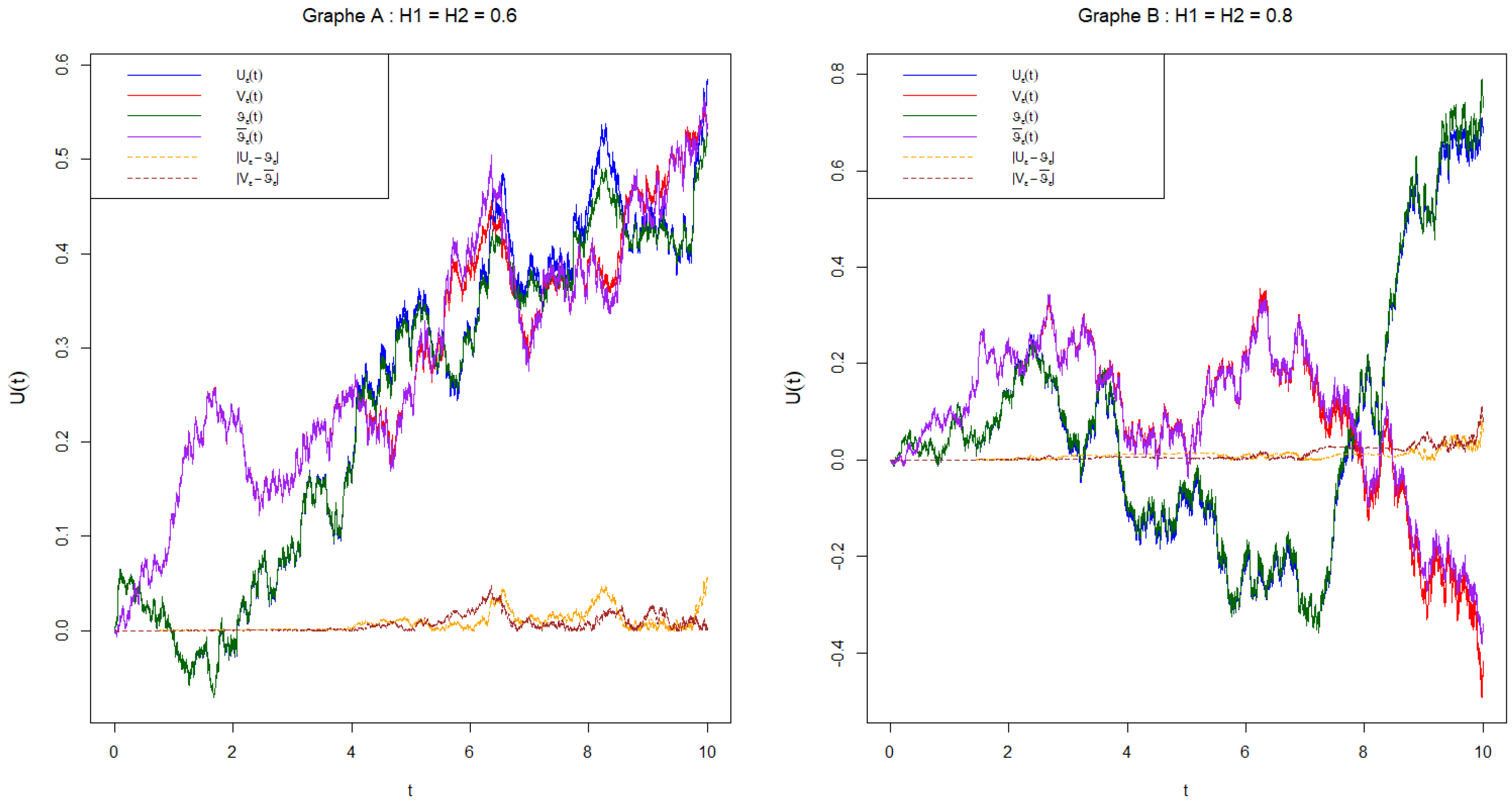
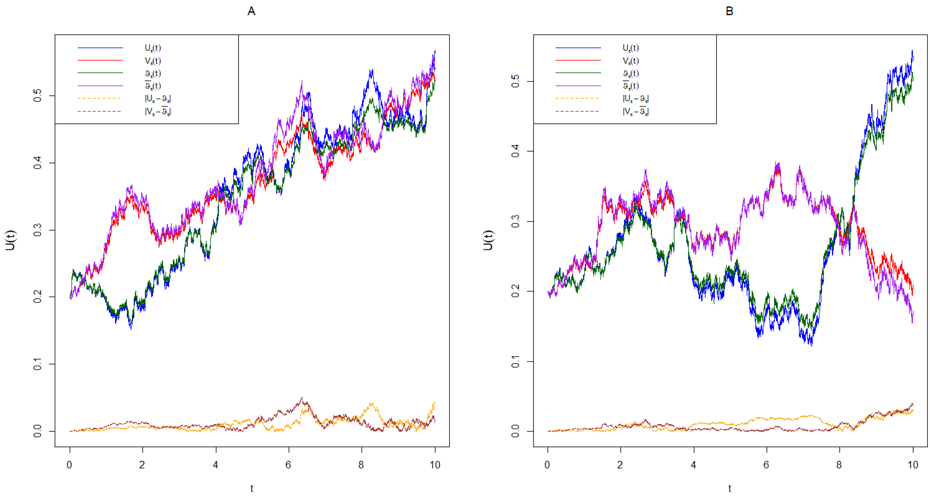
Now we have two examples to demonstrate the procedure of the averaging principle.

4.1. Example 1

Consider the following system:

$$\left\{\begin{array}{cc}d{U}_{ϵ}\hfill & =-{ϵ}^{2H}\eta (U_{ϵ}+V_{ϵ}+{\displaystyle \frac{U_{ϵ}{V}_{ϵ}}{2}}){sin}^2\left(t\right)dt+{\displaystyle \frac{{ϵ}^H}{2}}(1+U_{ϵ}{V}_{ϵ})d^{\circ }{B}^{H_1}\left(t\right)+{\displaystyle \frac{{ϵ}^H}{2}}d{L}_1\left(t\right)\hfill \\ \\ d{V}_{ϵ}\hfill & =-{ϵ}^{2H}\eta (U_{ϵ}+V_{ϵ}-{\displaystyle \frac{U_{ϵ}{V}_{ϵ}}{2}}){sin}^2\left(t\right)dt+{\displaystyle \frac{{ϵ}^H}{2}}(1-U_{ϵ}{V}_{ϵ})d^{\circ }{B}^{H_2}\left(t\right)+{\displaystyle \frac{{ϵ}^H}{2}}d{L}_2\left(t\right),\hfill \end{array}\right.$$

where $(U_{ϵ}\left(0\right),V_{ϵ}\left(0\right))=(u_0,v_0)$ denotes the initial condition with $\left(E\right|u_0{|}^2,E\left|v_0{|}^2\right)<(\infty ,\infty )$. Here,

$$b^1(t,U_{ϵ},V_{ϵ})=-\eta (U_{ϵ}+V_{ϵ}+{\displaystyle \frac{U_{ϵ}{V}_{ϵ}}{2}}){sin}^2\left(t\right)$$

and

$$b^2(t,U_{ϵ},V_{ϵ})=-\eta (U_{ϵ}+V_{ϵ}-{\displaystyle \frac{U_{ϵ}{V}_{ϵ}}{2}}){sin}^2\left(t\right),$$

$$A^1(t,U_{ϵ},V_{ϵ})=({\displaystyle \frac{1+U_{ϵ}{V}_{ϵ}}{2}}),$$

and

$$A^2(t,U_{ϵ},V_{ϵ})=({\displaystyle \frac{1-U_{ϵ}{V}_{ϵ}}{2}}),$$

$${\sigma }^2(t,U_{ϵ},V_{ϵ})={\sigma }^1(t,U_{ϵ},V_{ϵ})={\displaystyle \frac{1}{2}},$$

where $\eta \in (0,+\infty )$ and $L\left(t\right)=L_1\left(t\right)=L_2\left(t\right)$ is a Lévy motion with no Gaussian (Brownian) and $B^{H_1}\left(t\right)=B^{H_2}\left(t\right)=B^H\left(t\right)$ is a fractional Brownian motion.

Let

$${\overline{b}}^1(U_{ϵ},V_{ϵ})={\displaystyle \frac{1}{\pi }}{\int }_0^{\pi }{b}^1(t,U_{ϵ},V_{ϵ})dt=-{\displaystyle \frac{\eta }{2}}(U_{ϵ}+V_{ϵ}+{\displaystyle \frac{U_{ϵ}{V}_{ϵ}}{2}}),$$

$${\overline{b}}^2(U_{ϵ},V_{ϵ})={\displaystyle \frac{1}{\pi }}{\int }_0^{\pi }{b}^2(t,U_{ϵ},V_{ϵ})dt=-{\displaystyle \frac{\eta }{2}}(U_{ϵ}+V_{ϵ}-{\displaystyle \frac{U_{ϵ}{V}_{ϵ}}{2}}),$$

and

$${\overline{\sigma }}^1(U_{ϵ},V_{ϵ})={\displaystyle \frac{1}{\pi }}{\int }_0^{\pi }{\sigma }^1(t,U_{ϵ},V_{ϵ})dt={\displaystyle \frac{1+U_{ϵ}{V}_{ϵ}}{2}},$$

$${\overline{\sigma }}^2(U_{ϵ},V_{ϵ})={\displaystyle \frac{1}{\pi }}{\int }_0^{\pi }{\sigma }^2(t,U_{ϵ},V_{ϵ})dt={\displaystyle \frac{1-U_{ϵ}{V}_{ϵ}}{2}},$$

and

$${\overline{A}}^2(U_{ϵ},V_{ϵ})={\overline{A}}^1(U_{ϵ},V_{ϵ})={\displaystyle \frac{1}{2}}.$$

Let the new averaged SDEs be expressed as

$$\left\{\begin{array}{cc}d{\vartheta }_{ϵ}\left(t\right)\hfill & ={\epsilon }^{2H}{\overline{b}}^1(U_{ϵ}\left(t-\right),V_{ϵ}\left(t-\right))dt+{\epsilon }^H{\overline{\sigma }}^1\left(U_{ϵ}\left(t-\right)\right),V_{ϵ}\left(t-\right))d{L}_1\left(t\right)\hfill \\ \\ & +{\epsilon }^H{\overline{A}}^1(U_{ϵ}\left(t-\right),V_{ϵ}\left(t-\right))d^{\circ }{B}^{H_1}\left(t\right),t\in [0,T]\hfill \\ \\ d{\overline{\vartheta }}_{ϵ}\left(t\right)\hfill & ={\epsilon }^{2H}{\overline{b}}^2(U_{ϵ}\left(t-\right),V_{ϵ}\left(t-\right))dt+{\epsilon }^H{\overline{\sigma }}^2\left(U_{ϵ}\left(t-\right)\right),V_{ϵ}\left(t-\right))d{L}_2\left(t\right)\hfill \\ \\ & +{\epsilon }^H{\overline{A}}^2(U_{ϵ}\left(t-\right),V_{ϵ}\left(t-\right))d^{\circ }{B}^{H_2}\left(t\right),t\in [0,T].\hfill \end{array}\right.$$

Namely,

$$\left\{\begin{array}{cc}d{\vartheta }_{ϵ}\left(t\right)\hfill & =-{\epsilon }^{2H}{\displaystyle \frac{\eta }{2}}({\vartheta }_{ϵ}+{\overline{\vartheta }}_{ϵ}+{\displaystyle \frac{{\vartheta }_{ϵ}{\overline{\vartheta }}_{ϵ}}{2}})dt+{\displaystyle \frac{{\epsilon }^H}{2}}d{L}_1\left(t\right)\hfill \\ \\ & +{\epsilon }^H({\displaystyle \frac{1-{\vartheta }_{ϵ}{\overline{\vartheta }}_{ϵ}}{2}})d^{\circ }{B}^{H_1}\left(t\right),t\in [0,T]\hfill \\ \\ d{\overline{\vartheta }}_{ϵ}\left(t\right)\hfill & =-{\epsilon }^{2H}{\displaystyle \frac{\eta }{2}}({\vartheta }_{ϵ}+{\overline{\vartheta }}_{ϵ}-{\displaystyle \frac{{\vartheta }_{ϵ}{\overline{\vartheta }}_{ϵ}}{2}})dt+{\displaystyle \frac{{\epsilon }^H}{2}}d{L}_2\left(t\right)\hfill \\ \\ & +{\epsilon }^H({\displaystyle \frac{1+{\vartheta }_{ϵ}{\overline{\vartheta }}_{ϵ}}{2}})d^{\circ }{B}^{H_2}\left(t\right),t\in [0,T].\hfill \end{array}\right.$$

Obviously,

$${\tilde{\vartheta }}_{ϵ}\left(t\right)={\vartheta }_{ϵ}\left(t\right)+{\overline{\vartheta }}_{ϵ}\left(t\right),$$

is the well-known Ornstein–Uhlenbeck process, and the solution can be obtained as follows

$${\tilde{\vartheta }}_{ϵ}\left(t\right)=exp(-t{\epsilon }^{2H}\eta ){\tilde{\vartheta }}_0+{\epsilon }^H{\int }_0^{t}exp(-{\epsilon }^{2H}\eta (t-s))d^{\circ }{B}^H\left(t\right)+{\epsilon }^H{\int }_0^{t}exp(-{\epsilon }^{2H}\eta (t-s))dL\left(t\right).$$

Conditions $\left(Hyp1\right)$–$\left(Hyp5\right)$ are satisfied for ${\overline{b}}^l,b^l,{\overline{\sigma }}^l,{\sigma }^l,{\overline{A}}^l,A^l$ in SDEs (29) for each $l=1,2$, (30). Thus, Theorem 3 and Theorem 4 hold. Then

$$E\left(\underset{t\in [0,L{ϵ}^{-H\beta }]}{sup}|U_{ϵ}-{\vartheta }_{ϵ}|\right)\le {\delta }_1,$$

and

$$E\left(\underset{t\in [0,L{ϵ}^{-H\beta }]}{sup}|V_{ϵ}-{\overline{\vartheta }}_{ϵ}|\right)\le {\delta }_2.$$

Letting $ϵ\to 0$, we arrive at

$$U_{ϵ}\to {\vartheta }_{ϵ}\mathrm{in}\mathrm{probability},$$

and

$$V_{ϵ}\to {\overline{\vartheta }}_{ϵ}\mathrm{in}\mathrm{probability}.$$

Now we carry out the numerical simulation to obtain the solutions of example 1 under the conditions $H_1=H_2=0.6$, $ϵ=0.01$, $\lambda =1$ and $H_1=H_2=0.8$, $ϵ=0.01$, and $\lambda =1$, respectively. Figure 1A,B shows the comparison of exact solution $(U_{ϵ}\left(t\right),V_{ϵ}\left(t\right))$ with averaged solution $({\vartheta }_{ϵ},{\overline{\vartheta }}_{ϵ})$ as an example. One can see a good agreement between solutions of the original equation and the averaged equation.

Also, under the same conditions where $ϵ=0.0045$ and $U_{ϵ}\left(0\right)=V_{ϵ}\left(0\right)=0.2$., Figure 2A,B shows the comparison of exact solution $(U_{ϵ}\left(t\right),V_{ϵ}\left(t\right))$ with averaged solution $({\vartheta }_{ϵ},{\overline{\vartheta }}_{ϵ})$ as an example. One can see a good agreement between solutions of the original equation and the averaged equation.

To assess the effectiveness of the averaging method, we investigate how different parameter values affect the total error between the exact and averaged solutions. The parameters under consideration are:

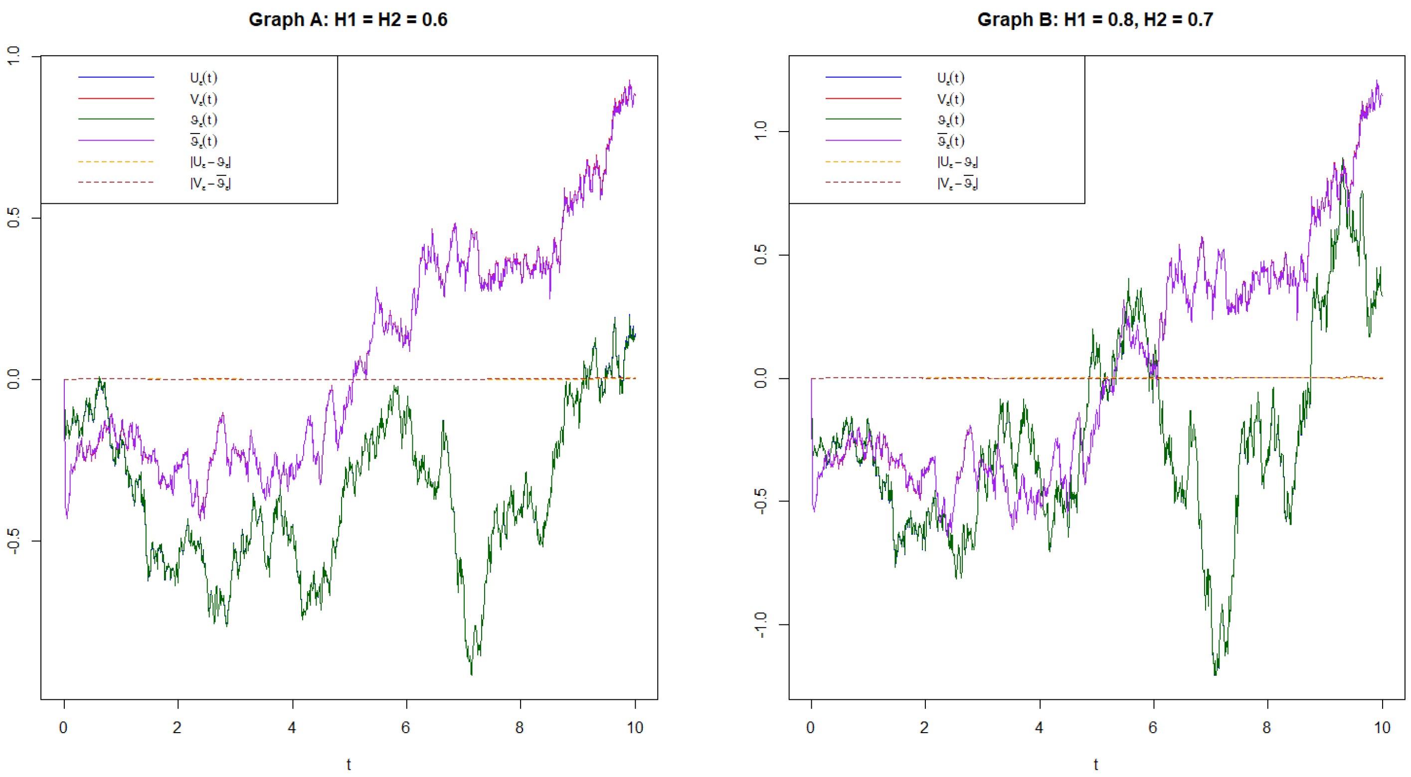
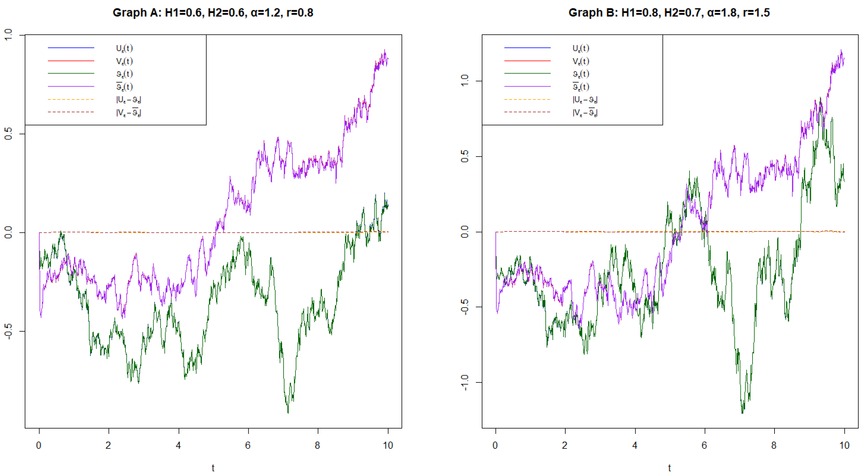
• $H_1$ and $H_2$: Hurst parameters related to the roughness of the fractional Brownian motion.
• $\lambda$: A scaling or regularization parameter.
• Total Error: A numerical measure of the discrepancy between the true and averaged solutions.

The

Table 1. Comparison of total errors for different values of $H_1$, $H_2$, and $\lambda$.

${\mathit{H}}_1$	${\mathit{H}}_2$	$\mathit{\lambda }$	Total Error
0.6	0.6	1.0	0.0231
0.7	0.6	0.5	0.0258
0.6	0.7	1.5	0.0283
0.7	0.7	1.0	0.0302
0.8	0.6	1.0	0.0320

presents the results of this analysis.

4.2. Example 2

Consider the following SDEs with $\alpha$ stable Lévy motion

$$\left\{\begin{array}{cc}d{U}_{ϵ}\hfill & ={\displaystyle \frac{{ϵ}^{2H}}{2}}(1-U_{ϵ}{V}_{ϵ})dt+{\displaystyle \frac{{ϵ}^H}{2}}{d}^{\circ }{B}^{H_1}\left(t\right)+{\displaystyle \frac{{ϵ}^H}{4}}(3-U_{ϵ}{V}_{ϵ})d{W}_1\left(t\right)\hfill \\ \hfill & +{ϵ}^H{\int }_{0<x<c}{x}^3(U_{ϵ}+V_{ϵ}){cos}^2(t+U_{ϵ}){\nu }_{\alpha }\left(dx\right)dt\hfill \\ \\ d{V}_{ϵ}\hfill & ={\displaystyle \frac{{ϵ}^{2H}}{2}}(1+U_{ϵ}{V}_{ϵ})dt+{\displaystyle \frac{{ϵ}^H}{2}}{d}^{\circ }{B}^{H_2}\left(t\right)+{\displaystyle \frac{{ϵ}^H}{4}}(1+U_{ϵ}{V}_{ϵ})d{W}_2\left(t\right)\hfill \\ \hfill & +{ϵ}^H{\int }_{0<x<c}{x}^3(U_{ϵ}+V_{ϵ}){cos}^2(t+V_{ϵ}){\nu }_{\alpha }\left(dx\right)dt,\hfill \end{array}\right.$$

(31)

where ${\nu }_{\alpha }\left(dx\right)={\displaystyle \frac{r}{x^{1+\alpha }}}dx$ denotes the $\alpha$-stable Lévy jump measure on $(0,\infty )$, $0<\alpha <2,r>0$, $(U_{ϵ}\left(0\right),V_{ϵ}\left(0\right))=(u_0,v_0)$, denoting the initial condition with

$$E|u_0{|}^2<\infty ,E{\left|v_0\right|}^2<\infty .$$

Putting

$$b^1(t,U_{ϵ},V_{ϵ})={\displaystyle \frac{1-U_{ϵ}{V}_{ϵ}}{2}},$$

$$b^2(t,U_{ϵ},V_{ϵ})={\displaystyle \frac{1+U_{ϵ}{V}_{ϵ}}{2}},$$

and

$$g^1(t,U_{ϵ},V_{ϵ})={\displaystyle \frac{3-U_{ϵ}{V}_{ϵ}}{4}},$$

$$g^2(t,U_{ϵ},V_{ϵ})={\displaystyle \frac{1+U_{ϵ}{V}_{ϵ}}{4}},$$

$$A^1(t,U_{ϵ},V_{ϵ})=A^1(t,U_{ϵ},V_{ϵ})={\displaystyle \frac{1}{2}},$$

$$G^1(t,U_{ϵ},V_{ϵ},x)=x^3(U_{ϵ}+V_{ϵ}){cos}^2,(t+U_{ϵ})$$

$$G^2(t,U_{ϵ},V_{ϵ},x)=x^3(U_{ϵ}+V_{ϵ}){cos}^2(t+V_{ϵ}),$$

and the other parameters are the same as in (8). Let

$$G^1({\vartheta }_{ϵ},{\overline{\vartheta }}_{ϵ},x)={\displaystyle \frac{1}{\pi }}{\int }_0^{\pi }{G}^1(t,U_{ϵ},V_{ϵ},x)dt={\displaystyle \frac{x^3(U_{ϵ}+V_{ϵ})}{2}},$$

and

$$G^2({\vartheta }_{ϵ},{\overline{\vartheta }}_{ϵ},x)={\displaystyle \frac{1}{\pi }}{\int }_0^{\pi }{G}^1(t,U_{ϵ},V_{ϵ},x)dt={\displaystyle \frac{x^3(U_{ϵ}+V_{ϵ})}{2}}.$$

After calculations,

$$\left\{\begin{array}{cc}d{\vartheta }_{ϵ}\hfill & ={\displaystyle \frac{{ϵ}^{2H}}{2}}(1-{\vartheta }_{ϵ}{\overline{\vartheta }}_{ϵ})dt+{\displaystyle \frac{{ϵ}^H}{2}}{d}^{\circ }{B}^{H_1}\left(t\right)+{\displaystyle \frac{{ϵ}^H}{4}}(3-{\vartheta }_{ϵ}{\overline{\vartheta }}_{ϵ})d{W}_1\left(t\right)\hfill \\ \hfill & +{\displaystyle \frac{{ϵ}^H}{2}}{\int }_{0<x<c}{x}^3({\vartheta }_{ϵ}+{\overline{\vartheta }}_{ϵ}){\nu }_{\alpha }\left(dx\right)dt\hfill \\ \\ d{\overline{\vartheta }}_{ϵ}\hfill & ={\displaystyle \frac{{ϵ}^{2H}}{2}}(1+{\vartheta }_{ϵ}{\overline{\vartheta }}_{ϵ})dt+{\displaystyle \frac{{ϵ}^H}{2}}{d}^{\circ }{B}^{H_2}\left(t\right)+{\displaystyle \frac{{ϵ}^H}{4}}(1+{\vartheta }_{ϵ}{\overline{\vartheta }}_{ϵ})d{W}_2\left(t\right)\hfill \\ \hfill & +{\displaystyle \frac{{ϵ}^H}{2}}{\int }_{0<x<c}{x}^3({\vartheta }_{ϵ}+{\overline{\vartheta }}_{ϵ}){\nu }_{\alpha }\left(dx\right)dt.\hfill \end{array}\right.$$

(32)

Now we define a new (averaged) SDEs as

$$d{\tilde{\vartheta }}_{ϵ}={ϵ}^H({ϵ}^H+\beta {\tilde{\vartheta }}_{ϵ})dt+{ϵ}^H{d}^{\circ }{B}^H\left(t\right)+{ϵ}^{H}dW\left(t\right),$$

where

$$\beta ={\displaystyle \frac{r{c}^{3-\alpha }}{3-\alpha }}>0.$$

Thus problem (32) is a linear SDE and its solution (see [25]). All the conditions $\left(Hyp1\right)-\left(C5\right)$ are satisfied for functions ${\overline{b}}^l,b^l,{\overline{\sigma }}^l,{\sigma }^l,{\overline{A}}^l,A^l$ where $l=1,2$, so we can use the solution $({\vartheta }_{ϵ},{\overline{\vartheta }}_{ϵ})$ to approximate the original solution $(U_{ϵ},V_{ϵ})$ to the SDEs (31), and the convergence in mean square and in probability will be assured.

In Figure 3A,B and Figure 4A,B, we present numerically the comparisons between the solution $(U_{ϵ}\left(t\right),V_{ϵ}\left(t\right))$ of the original example 2 and the solution $({\vartheta }_{ϵ},{\overline{\vartheta }}_{ϵ})$ of the averaged example 2, with the same initial conditions $H_1=H_2=0.6$, $ϵ=0.1$, $\alpha =1$, $r=1, c=1$. The other parameter values are taken as $H_1=0.8, H_2=0.7$, $ϵ=0.1$, $\alpha =1$, $r=1, c=1$. respectively. From Figure 3A,B, good agreements can be found between these solutions for $(U_{ϵ}\left(t\right),V_{ϵ}\left(t\right))$ and $({\vartheta }_{ϵ},{\overline{\vartheta }}_{ϵ})$.

Table 2. Comparison of errors for different parameter configurations.

${\mathit{H}}_1$	${\mathit{H}}_2$	$\mathit{\alpha }$	r	$\mathit{\lambda }$	Error_U	Error_V
0.8	0.6	1.8	0.5	3	0.0008456	0.0007523
0.7	0.6	1.8	0.5	3	0.0009262	0.0006721
0.7	0.6	1.5	0.5	3	0.0009491	0.0006868
0.8	0.6	1.5	0.5	3	0.0008642	0.0007743
0.6	0.6	1.8	0.5	3	0.0010092	0.0006508
0.6	0.6	1.2	1.0	3	0.0009149	0.0007603
0.6	0.6	1.2	1.5	3	0.0009149	0.0007603
0.6	0.6	1.5	1.0	3	0.0009149	0.0007603
0.6	0.6	1.5	1.5	3	0.0009149	0.0007603
0.6	0.6	1.8	1.0	3	0.0009149	0.0007603

presents a comparison of the errors in $(U_{ϵ}\left(t\right),V_{ϵ}\left(t\right))$ for different parameter configurations, including variations in $H_1$, $H_2$, $\alpha$, r and $\lambda$.

5. Conclusions

The purpose of this paper is to establish an averaging principle for stochastic differential equations with non-Gaussian Lévy noise. The solutions to stochastic systems with Lévy noise can be approximated by solutions to averaged stochastic differential equations in the sense of both convergence in mean square and convergence in probability. The convergence order is also estimated in terms of noise intensity.

The novelty of combining Lévy noise with the FBMin averaging principles is the following:

Lack of Unified Framework for Mixed Lévy noise and fBm.

Most results in the literature treat Lévy noise and fBm separately due to their fundamentally different properties, outlined as follows:

(A)

Lévy processes are discontinuous and Markovian.

(B)

FBm is continuous but non-Markovian and not a semimartingale when $H\ne {\displaystyle \frac{1}{2}}$.

(C)

There is a shortage of rigorous frameworks and solution theories for SDEs that simultaneously handle non-Markovian memory and jumps.

While averaging principles have been studied for SDEs with Lévy noise [14] and separately for fBm [23], few studies address multi-scale systems driven by both types of noise.

Gap: Lack of multi-scale stochastic averaging theory for hybrid systems combining long-term memory and jump behavior.

References

- Nualart, D.; Schoutens, W. Chaotic and predictable representation for Lévy processes. Stoch. Process. Their Appl. 2000, 90, 109–122. [Google Scholar] [CrossRef]
- Applebaum, D. Lévy Processes and Stochastic Calculus, 2nd ed.; Cambridge University Press: Cambridge, UK, 2009. [Google Scholar]
- Bertoin, J. Lévy Processes; Cambridge University Press: Cambridge, UK, 1998. [Google Scholar]
- Bogoliubov, N.N.; Krylov, N.M. La theorie generale de la mesure dans son application a l’etude de systemes dynamiques de la mecanique non-lineaire. Ann. Math. 1937, 38, 65–113. [Google Scholar]
- Kunita, H. Stochastic differential equations based on Lévy processes and stochastic flows of diffeomorphisms. In Real and Stochastic Analysis; Rao, M.M., Ed.; Birkhiuser: Boston, MA, USA, 2004; pp. 305–373. [Google Scholar]
- Zhu, W.Q. Nonlinear stochastic dynamics and control in Hamiltonian formulation. ASME Appl. Mech. Rev. 2006, 59, 230–248. [Google Scholar] [CrossRef]
- Zeng, Y.; Zhu, W.Q. Stochastic Averageing of Quasi-Nonintegrable- Hamiltonian Systems Under Poisson White Noise Excitation. J. Apple. Mech.-Trans. ASME 2011, 78, 021002–021011. [Google Scholar] [CrossRef]
- Stoyanov, I.M.; Bainov, D.D. The averaging method for a class of stochastic differential equations. Ukr. Math. J. 1974, 26, 186–194. [Google Scholar] [CrossRef]
- Xu, Y.; Pei, B.; Li, Y. Approximation properties for solutions to non-Lipschitz stochastic differential equations with Levy noise. Math. Meth. Appl. Sci. 2015, 38, 2120–2131. [Google Scholar] [CrossRef]
- Liu, X.; Duan, J.; Liu, J.; Kloeden, P. Synchronization of dissipative dynamical systems driven by non-Gaussian Lévy noises. Int. J. Stoch. Anal. 2010, 2010, 502803. [Google Scholar] [CrossRef]
- Hu, Y.; Øksendal, B. Fractional white noise calculus and application to finance. Infin. Dimens. Anal. Quantum Probab. Relat. Topics 2003, 6, 1–32. [Google Scholar] [CrossRef]
- Tudor, C.A. Analysis of Variations for Self-Similar Processes: A Stochastic Calculus Approach; Springer: Berlin/Heidelberg, Germany, 2013. [Google Scholar]
- Xu, Y.; Guo, R.; Liu, D.; Zhang, H.; Duan, J. Stochastic averaging principle for dynamical systems with fractional Brownian motion. arXiv 2013, arXiv:1301.4788. [Google Scholar] [CrossRef]
- Ren, L.; Xiao, G. The Averaging Principle for Caputo Type Fractional Stochastic Differential Equations with Lévy Noise. Fractal Fract. 2024, 8, 595. [Google Scholar] [CrossRef]
- Xu, W.; Duan, J.; Xu, W. An averaging principle for fractional stochastic differential equations with Lévy noise. Chaos 2020, 30, 083126. [Google Scholar] [CrossRef] [PubMed]
- Ikeda, N.; Watanabe, S. Stochastic Differential Equations and Diffusion Processes; North Holland Publishing Company: Amsterdam, The Netherlands; Oxford, UK; New York, NY, USA, 1989. [Google Scholar]
- Blouhi, T.; Ferhat, M. Coupled System of Second-Order Stochastic Differential Inclusions Driven by Levy Noise. Mem. Differ. Equ. Math. Phys. 2024, f91, 21–38. [Google Scholar]
- Ferha, M.; Blouhi, T. Topological method for coupled systems of impulsive neutral functional differential inclusions driven by a fractional Brownian motion and Wiener process. Filomat 2024, 38, 6193–6217. [Google Scholar] [CrossRef]
- Alos, E.; Nualart, D. Stochastic calculus with respect to the fractional Brownian motion. Ann. Probab. 2001, 29, 766–801. [Google Scholar] [CrossRef]
- Bihari, I. A generalisation of a lemma of Bellman and its application to uniqueness problems of differential equations. Acta Math. Acad. Sci. Hungar. 1956, 7, 81–94. [Google Scholar] [CrossRef]
- Biagini, F.; Hu, Y.; Øksendal, B.; Zhang, T. Stochastic Calculus for Fractional Brownian Motion and Applications; Springer: London, UK, 2008. [Google Scholar]
- Taniguchi, T. The existence and asymptotic behaviour of solutions to non-Lipschitz stochastic functional evolution equations driven by Poisson jumps. Stochastics 2010, 82, 339–363. [Google Scholar] [CrossRef]
- Xu, Y.; Duan, J.; Xu, W. An averaging principle for stochastic dynamical systems with Levy noise. Phys. D Nonlinear Phenom. 2011, 240, 1395–1401. [Google Scholar] [CrossRef]
- Wang, L.; Cheng, T.; Zhang, Q. Successive approximation to solutions of stochastic differential equations with jumps in local non-Lipschitz conditions. Appl. Math. Comp. 2013, 225, 142–150. [Google Scholar] [CrossRef]
- Klebaner, F.C. Introduction to Stochastic Calculus with Applications, 2nd ed.; Imperial College Press: London, UK, 2005. [Google Scholar]