Ulam–Hyers Stability of Fractional Difference Equations with Hilfer Derivatives

Abstract

This paper investigates the Ulam–Hyers stability of both linear and nonlinear delayed neutral Hilfer fractional difference equations. We utilize the nabla Laplace transform, known as the N-transform, along with a generalized discrete Gronwall inequality to derive sufficient conditions for stability. For the linear case, we provide an explicit solution formula involving discrete Mittag-Leffler functions and establish its stability properties. In the nonlinear case, we concentrate on delayed neutral Hilfer fractional difference equations, a class of systems that appears to be unexplored in the existing literature with respect to Ulam–Hyers stability. In particular, for the linear case, the absolute difference between the solution of the linear Hilfer fractional difference equation and the solution of the corresponding perturbed equation is bounded by the function of $\epsilon$ when the perturbed term is bounded by $\epsilon$. In the case of the neutral fractional delayed Hilfer difference equation, the absolute difference is bounded by a constant multiple of $\epsilon$. Our results fill this gap by offering novel stability criteria. We support our theoretical findings with illustrative numerical examples and simulations, which visually confirm the predicted stability behavior and demonstrate the applicability of the results in discrete fractional dynamic systems.

1. Introduction

Fractional difference equations naturally extend classical difference equations, incorporating the concept of fractional calculus into discrete settings. These equations provide a powerful framework for modeling systems that exhibit memory effects and long-range dependencies, making them highly relevant in various scientific and engineering fields. Unlike integer-order difference equations, which rely on discrete changes over fixed steps, fractional difference equations allow for non-integer orders of differentiation and enable more flexible and accurate descriptions of complex dynamical behaviors.

The applications of fractional difference equations span multiple disciplines, including finance, where they are used to model long-memory processes in stock market analysis; control theory, where they improve the stability and efficiency of control systems; and biology, e.g., where they describe population dynamics with hereditary effects. Their ability to capture memory-dependent processes makes them particularly valuable in areas where past states influence future behavior in a non-trivial manner. We refer to the pioneering book in [1] for an elaborative review on discrete fractional calculus.

The Hilfer approach in fractional calculus bridges the gap between the widely used Riemann–Liouville and Caputo fractional derivatives [2]. This approach provides a more flexible framework for modeling complex systems where the order of differentiation and the weighting of initial conditions play crucial roles. The Hilfer fractional derivative is a two-parameter operator, defined by incorporating an additional parameter that controls the interpolation between the Riemann–Liouville and Caputo fractional derivatives. This added flexibility makes it particularly useful in applications where both global and local memory effects need to be accounted for simultaneously. One of the key advantages of the Hilfer fractional derivative is its ability to describe anomalous diffusion processes and other physical phenomena where traditional fractional derivatives fail to provide an accurate representation. It has been widely applied in various fields such as viscoelasticity, signal processing, and mathematical physics, where systems exhibit intermediate behavior between purely local and fully history-dependent dynamics. By allowing for a smooth transition between different types of fractional derivatives, the Hilfer approach enhances the modeling capabilities of fractional calculus, providing a richer and more adaptable mathematical framework. As a result, it has gained significant attention in the study of fractional differential equations and their applications in science and engineering. The Hilfer approach in fractional calculus has been adapted to discrete settings, and Hilfer nabla fractional difference equations extend the classical discrete fractional calculus by incorporating this approach into the nabla difference operator.

As in the continuous case, Hilfer nabla fractional difference operators depend on two parameters, which allows for a smooth transition between Riemann–Liouville and Caputo nabla fractional differences. Hilfer nabla fractional difference equations, formulated using this operator, serve as powerful tools in discrete dynamic modeling, particularly in fields such as discrete control theory, signal processing, and biological systems, where backward differences are more suitable for capturing past-dependent processes. We refer readers to the research articles [3,4,5] for the adaptation of Hilfer fractional derivatives in a discrete setting, and we also recommend the papers [6,7] regarding the existence and asymptotic behavior of the solutions of Hilfer fractional difference equations as further information in this direction.

The stability of fractional difference equations is crucial for understanding the long-term behavior of discrete systems governed by fractional dynamics. Unlike integer-order difference equations, which describe systems with memoryless evolution, fractional difference equations incorporate memory effects, making their stability analysis more complex and significant. Stability ensures that small changes in the initial conditions or external perturbations do not lead to unbounded or erratic behavior in the system over time. This is particularly important in applications such as control theory, signal processing, finance, and biological models, where stable solutions guarantee reliable predictions and robust system performance. Different notions of stability, such as asymptotic, exponential, and practical stability, are studied to assess the behavior of solutions under various conditions.

Among the different stability concepts, Ulam–Hyers stability plays a fundamental role in the analysis of fractional difference equations. This type of stability, originally introduced by Ulam and later formalized by Hyers, addresses the question of whether an approximate solution to a given equation can be close to an exact solution within a controlled margin. In the context of fractional difference equations, Ulam–Hyers stability provides insights into how errors or small perturbations in the initial conditions affect the overall dynamics of the system. A system that satisfies Ulam–Hyers stability ensures that solutions remain within a bounded deviation from the true solution, making it particularly useful in numerical approximations and real-world applications where data imperfections are inevitable. The concept is further extended to generalized Ulam–Hyers stability, which accounts for more flexible error bounds and varying perturbation constraints. Understanding and applying Ulam–Hyers stability in fractional difference equations contribute to the development of reliable mathematical models, ensuring their robustness and applicability in practical scenarios. The literature on Ulam–Hyers stability is vast. We bring the papers [8,9,10,11] into the spotlight, which concentrate on the Ulam–Hyers stability of fractional difference equations, and we also refer to [12,13,14,15] as inspiring papers on the Ulam–Hyers stability of fractional equations with delay, boundary conditions, and impulse.

In this paper, we concentrate on the Ulam–Hyers stability of both linear and nonlinear delayed neutral Hilfer fractional difference equations. In the linear case, we use the $\mathcal{N}$-transform in order to show that the linear Hilfer fractional difference equation is Ulam–Hyers stable under certain conditions. Subsequently, we turn our attention to nonlinear delayed neutral Hilfer fractional difference equations and their Ulam–Hyers stability. Despite the fact that there are numerous studies on the Ulam–Hyers stability of nonlinear Hilfer fractional difference equations, neutral-type equations have not been studied in the existing literature to the best of our knowledge. Thus, we aim to fill this gap and obtain the sufficient conditions for the Ulam–Hyers stability of neutral Hilfer fractional difference equations by following a different approach to that of the linear equations.

The organization of this manuscript is briefly described as follows: In the subsequent section, we give the preliminaries of nabla fractional calculus and Hilfer-like discrete fractional calculus. In Section 3, we present the main stability outcomes; finally, in the last section, we provide some examples as an implementation of the main results.

2. Essentials on Discrete Fractional Calculus

This section is devoted to the presentation of the preliminaries of nabla fractional calculus for potential readers who may not be familiar with the theory of discrete fractional calculus. The following milestone content is borrowed from the monograph [1] and the papers [16,17]. Throughout the manuscript, we use the notations ${\mathbb{N}}_a$ and ${\mathbb{N}}_a^{\delta }$ for any a, $\delta \in \mathbb{R}$ such that $\delta -a\in {\mathbb{N}}_1$ to express the sets $\left\{a,a+1,a+2,\cdots \right\}$ and $\left\{a,a+1,a+2,\cdots ,\delta \right\},$ respectively.

In discrete (fractional) calculus, the backward jump operator $\rho :{\mathbb{N}}_{a+1}\to {\mathbb{N}}_a$ is given by $\rho \left(t\right)=t-1,$ $t\in {\mathbb{N}}_{a+1}.$ The first-order nabla difference of $f:{\mathbb{N}}_a\to \mathbb{R}$ is defined by $\nabla f:=f\left(t\right)-f\left(t-1\right)$ for $t\in {\mathbb{N}}_{a+1};$ the higher-order nabla differences of $f,$${\nabla }^{N}f,$ are defined recursively for $N\in {\mathbb{N}}_1.$ The ${\mu }^{th}$-order nabla fractional Taylor monomial is introduced as

$$H_{\mu }\left(t,a\right):={\displaystyle \frac{{\left(t-a\right)}^{\overline{\mu }}}{\mathsf{\Gamma }\left(\mu +1\right)}}:={\displaystyle \frac{\mathsf{\Gamma }\left(t-a+\mu \right)}{\mathsf{\Gamma }\left(t-a\right)\mathsf{\Gamma }\left(\mu +1\right)}},\mu \in \mathbb{R}\setminus \left\{\cdots ,-2,-1\right\},$$

provided that the right-hand side is well-defined. Additionally, the following Taylor monomials are well-defined:

Lemma 1 

([18]). Let $\upsilon >-1$ and $s\in {\mathbb{N}}_a.$ Then, the following holds:

(i) 

If $t\in {\mathbb{N}}_{\rho \left(s\right)},$ then $H_{\upsilon }\left(t,\rho \left(s\right)\right)\ge 0;$ moreover, if $t\in {\mathbb{N}}_s,$ then $H_{\upsilon }\left(t,\rho \left(s\right)\right)>0.$

(ii) 

If $t\in {\mathbb{N}}_{\rho \left(s\right)}$ and $\upsilon >0,$ then $H_{\upsilon }\left(t,\rho \left(s\right)\right)$ is a decreasing function of $s;$ if $t\in {\mathbb{N}}_s$ and $-1<\upsilon <0,$ then $H_{\upsilon }\left(t,\rho \left(s\right)\right)$ is an increasing function of $s.$

(iii) 

If $t\in {\mathbb{N}}_{\rho \left(s\right)}$ and $\upsilon \ge 0,$ then $H_{\upsilon }\left(t,\rho \left(s\right)\right)$ is a non-decreasing function of $t;$ if $\upsilon >0$ and $t\in {\mathbb{N}}_s,$ then $H_{\upsilon }\left(t,\rho \left(s\right)\right)$ is an increasing function of $t.$ Also, if $t\in {\mathbb{N}}_{s+1}$ and $-1<\upsilon <0,$ then $H_{\upsilon }\left(t,\rho \left(s\right)\right)$ is a decreasing function of $t.$

The ${\upsilon }^{th}$ nabla sum of f based at a is introduced as

$$\left({\nabla }_a^{-\upsilon }f\right)\left(t\right):={\displaystyle \sum _{s=a}^t}{H}_{\upsilon -1}\left(t,\rho \left(s\right)\right)f\left(s\right),t\in {\mathbb{N}}_a,$$

for any $f:{\mathbb{N}}_a\to \mathbb{R}.$ Two milestone definitions for fractional nabla differences, the so-called Riemann–Liouville nabla difference and Caputo nabla difference, are defined as follows: Let $\upsilon >0,$ $N\in {\mathbb{N}}_1$ and $N-1<\upsilon \le N.$ Then, we define the following:

Riemann–Liouville (R-L) nabla difference 

Suppose that $f:{\mathbb{N}}_a\to \mathbb{R}.$ Then, the R-L fractional difference of $f(·)$ is given by

$$\left({\nabla }_a^{\upsilon }f\right)\left(t\right):=\left({\nabla }^N\left({\nabla }_a^{-\left(N-\upsilon \right)}f\right)\right)\left(t\right),t\in {\mathbb{N}}_{a+N}.$$

(1)

Caputo nabla difference 

Let $f:{\mathbb{N}}_{a-N}\to \mathbb{R}.$ Then, the Caputo fractional difference of $f(·)$ is given by

$$\left({\nabla }_{*a}^{\upsilon }f\right)\left(t\right):=\left({\nabla }_a^{-\left(N-\upsilon \right)}\left({\nabla }^{N}f\right)\right)\left(t\right),t\in {\mathbb{N}}_a.$$

(2)

We need the following auxiliary results:

Lemma 2 

([1]). (i) Let $\upsilon >0$ and $\mu \in \mathbb{R}.$ Then, ${\nabla }_a^{-\upsilon }{H}_{\mu }\left(t,\rho \left(a\right)\right)=H_{\mu +\upsilon }\left(t,\rho \left(a\right)\right),$$t\in {\mathbb{N}}_a.$

(ii) Let $\upsilon ,\mu \in \mathbb{R},$$N\in {\mathbb{N}}_1$ and $N-1<\upsilon \le N.$ Then,

$${\nabla }_a^{\upsilon }{H}_{\mu }\left(t,\rho \left(a\right)\right)=H_{\mu -\upsilon }\left(t,\rho \left(a\right)\right),t\in {\mathbb{N}}_{a+N}.$$

We need the notion of the three-parameter Mittag-Leffler function $E_{p,\alpha ,\beta }(·,·)$:

Definition 1. 

Suppose that $\left|p\right|<1,\alpha >0,$ and $\beta \in \mathbb{R}.$ Then, the nabla Mittag-Leffler function is given by

$$E_{p,\alpha ,\beta }\left(t,a\right):={\displaystyle \sum _{k=0}^{\infty }}{p}^k{H}_{\alpha k+\beta }\left(t,a\right),t\in {\mathbb{N}}_a.$$

The infinite series on the right-hand side converges absolutely for $-1<p<1$.

We collect the main properties of function $E_{p,\alpha ,\beta }(·,·)$ in the next lemma:

Lemma 3 

([1,17]). Assume that $\left|p\right|<1,\alpha >0$ and $\beta \in \mathbb{R}.$ Then,

(i) 

${\nabla }_a^{-\upsilon }{E}_{p,\alpha ,\beta }\left(t,\rho \left(a\right)\right)=E_{p,\alpha ,\beta +\upsilon }\left(t,\rho \left(a\right)\right),$ $t\in {\mathbb{N}}_a$ whenever $\upsilon >0.$

(ii) 

${\nabla }_a^{\upsilon }{E}_{p,\upsilon ,\upsilon -1}\left(t,\rho \left(a\right)\right)=p{E}_{p,\upsilon ,\upsilon -1}\left(t,\rho \left(a\right)\right),$ $t\in {\mathbb{N}}_{a+1}$ whenever $0<\upsilon \le 1.$

(iii) 

$E_{p,\upsilon ,-1}\left(t,\rho \left(a\right)\right)=p{E}_{p,\upsilon ,\upsilon -1}\left(t,\rho \left(a\right)\right),$ $t\in {\mathbb{N}}_{a+1}$ whenever $0<\upsilon \le 1.$

Lemma 4 

([19]). Suppose that $0<b<1$ and $0<\upsilon <1.$ Then,

$$\underset{t\to \infty }{lim}{E}_{-b,\upsilon ,\upsilon -1}\left(t,\rho \left(a\right)\right)=0.$$

Theorem 1 

([20] Generalized Gronwall Inequality). Let $\alpha >0$ and $f(·)$ be a non-negative function. Suppose that $g(·)$ and $h(·)$ are non-negative and non-decreasing functions defined on ${\mathbb{N}}_0$ so that $h\left(t\right)\le M$ for all $t\in {\mathbb{N}}_0,$ where M is a constant. If

$$f\left(t\right)\le g\left(t\right)+h\left(t\right)\mathsf{\Gamma }\left(\alpha \right)\left({\nabla }_1^{-\alpha }f\right)\left(t\right),t\in {\mathbb{N}}_0,$$

then

$$f\left(t\right)\le g\left(t\right)E_{h\left(t\right)\mathsf{\Gamma }\left(\alpha \right),\alpha ,0}\left(t,0\right),t\in {\mathbb{N}}_0.$$

The $\mathcal{N}$-transform, also known as the nabla Laplace transform, serves as a powerful tool for solving discrete fractional difference equations, particularly those involving Hilfer-type operators. Its main advantage lies in its ability to convert complex fractional difference equations into algebraic equations in the transform domain, significantly simplifying the analysis. This transformation facilitates explicit solution representations, such as those involving discrete Mittag-Leffler functions, which naturally arise in the inverse transform. Compared to iterative or fixed-point techniques, the N-transform provides a more direct and constructive approach, especially for linear problems. Additionally, it offers the systematic handling of initial conditions, which is crucial in Hilfer-type problems, where the weighting of the initial data is parameter-dependent. Its efficiency, clarity, and suitability for deriving closed-form solutions make the N-transform preferable to many traditional analytical techniques in the discrete fractional setting.

In the following, we recall the basic details about the $\mathcal{N}$-transform of sequences and highlight its most important characteristics:

Definition 2. 

Let $f:{\mathbb{N}}_a\to \mathbb{R}$ be a function. Then, the nabla Laplace transform of f is given by

$${\mathcal{N}}_a\left[f\left(t\right)\right]:={\displaystyle \sum _{t=a}^{\infty }}{\left(1-s\right)}^{t-1}f\left(t\right),$$

if the infinite series converges.

Lemma 5 

([16,17]). Suppose that $f:{\mathbb{N}}_a\to \mathbb{R}.$ Then, we have

(i) 

${\mathcal{N}}_a\left[{\left(t-\rho \left(a\right)\right)}^{\overline{\mu -1}}\right]=\mathsf{\Gamma }\left(\mu \right){\left(1-s\right)}^{a-1}{s}^{-\mu }$ for $\mu \in \mathbb{R}\setminus \left\{\cdots ,-1,0\right\}.$

(ii) 

${\mathcal{N}}_a\left[H_{\mu -1}\left(t,\rho \left(a\right)\right)\right]={\left(1-s\right)}^{a-1}{s}^{-\mu }$ for $\mu \in \mathbb{R}\setminus \left\{\cdots ,-1,0\right\}.$

(iii) 

${\mathcal{N}}_a\left[\left({\nabla }_a^{-\upsilon }f\right)\left(t\right)\right]=s^{-\upsilon }{\mathcal{N}}_a\left[f\left(t\right)\right]$ for $\upsilon >0.$

(iv) 

${\mathcal{N}}_{a+1}\left[\left({\nabla }_a^{\upsilon }f\right)\left(t\right)\right]=s^{\upsilon }{\mathcal{N}}_a\left[f\left(t\right)\right]-{\left(1-s\right)}^{a-1}f\left(a\right)$ for $0<\upsilon \le 1.$

(v) 

${\mathcal{N}}_a\left[E_{p,\alpha ,\beta }\left(t,\rho \left(a\right)\right)\right]={\left(1-s\right)}^{a-1}{\displaystyle \frac{s^{\alpha -\beta -1}}{s^{\alpha }-p}},$$\left|s^{\alpha }p\right|<1.$

(vi) 

${\mathcal{N}}_1\left[E_{p,\alpha ,\beta }\left(t+a,a\right)\right]={\displaystyle \frac{s^{\alpha -\beta -1}}{s^{\alpha }-p}},$$\left|s^{\alpha }p\right|<1.$

Before presenting the formal definition, we provide an intuitive understanding of the Hilfer fractional difference operator in the discrete setting. In classical fractional calculus, the Hilfer operator acts as a bridge between the Riemann–Liouville and Caputo derivatives, blending local and global memory effects through a tunable parameter. Similarly, in the discrete case, the Hilfer fractional difference operator introduces a weighted interpolation between the Riemann–Liouville-type and Caputo-type nabla fractional differences. The interpolation parameter $\beta \in [0,1]$ controls the balance between the initial condition emphasis and the system’s memory—with $\beta =0$ recovering the Riemann–Liouville case and $\beta =1$ yielding the Caputo version. This flexibility makes the operator particularly suitable for modeling discrete-time systems with complex hereditary characteristics, where both the starting state and accumulated past behavior influence the present. Essentially, the Hilfer operator enriches the modeling toolkit by allowing for a continuum of behaviors between the two classical types.

The formal definition is as follows:

Definition 3 

([4], Hilfer nabla fractional difference). Let $f:{\mathbb{N}}_a\to \mathbb{R},$ $0\le \beta \le 1,$ $N\in {\mathbb{N}}_1$ and $N-1<\alpha \le N.$ Then, the ${\alpha }^{th}$-order, ${\beta }^{th}$-type Hilfer nabla fractional difference of f is given by

$$\left({\nabla }_a^{\alpha ,\beta }f\right)\left(t\right):=\left({\nabla }_{a+N}^{-\beta \left(N-\alpha \right)}{\nabla }^N{\nabla }_a^{-\left(1-\beta \right)\left(N-\alpha \right)}f\right)\left(t\right),t\in {\mathbb{N}}_{a+N}.$$

(3)

Note that the Hilfer nabla fractional difference operator defined in (3) is equal to the R-L nabla fractional difference in (1) when $\beta =0$, and it is also identical to the Caputo nabla fractional difference represented in (2) when $\beta =1.$

We conclude this section by presenting the following auxiliary results:

Lemma 6 

([4]). Let $\mu \in \mathbb{R},$ $0<\alpha \le 1,0\le \beta \le 1$ be such that the following fractional nabla Taylor monomials are well-defined. Then, we have

$${\nabla }_a^{\alpha ,\beta }{H}_{\mu }\left(t,\rho \left(a\right)\right)=H_{\mu -\alpha }\left(t,\rho \left(a\right)\right)-H_{\beta \left(1-\alpha \right)-1}\left(t,\rho \left(a\right)\right),t\in {\mathbb{N}}_{a+1}.$$

Lemma 7 

([4]). Let $f:{\mathbb{N}}_a\to \mathbb{R},$ $0<\alpha \le 1,$ $0\le \beta \le 1$ and $\gamma =\alpha +\beta -\alpha \beta .$ Then,

(i) 

$\left({\nabla }_a^{\alpha ,\beta }f\right)\left(t\right)=\left({\nabla }_{a+1}^{-\beta \left(1-\alpha \right)}{\nabla }_a^{\gamma }f\right)\left(t\right),$$t\in {\mathbb{N}}_{a+1}.$

(ii) 

$\left({\nabla }_{a+1}^{-\gamma }{\nabla }_a^{\gamma }f\right)\left(t\right)=\left({\nabla }_{a+1}^{-\alpha }{\nabla }_a^{\alpha ,\beta }f\right)\left(t\right),$$t\in {\mathbb{N}}_{a+1}.$

(iii) 

$\left({\nabla }_a^{\gamma }{\nabla }_a^{-\alpha }f\right)\left(t\right)=\left({\nabla }_a^{\beta \left(1-\alpha \right)}f\right)\left(t\right),$$t\in {\mathbb{N}}_{a+1}.$

(iv) 

$\left({\nabla }_a^{\alpha ,\beta }{\nabla }_a^{-\alpha }f\right)\left(t\right)=\left({\nabla }_{a+1}^{-\beta \left(1-\alpha \right)}{\nabla }_a^{\beta \left(1-\alpha \right)}f\right)\left(t\right),$$t\in {\mathbb{N}}_{a+1}.$

Lemma 8 

([4]). Let $0<\alpha \le 1$, $0\le \beta \le 1$ and $\gamma =\alpha +\beta -\alpha \beta .$ Then, we have

$${\mathcal{N}}_{a+1}\left[\left({\nabla }_a^{\alpha ,\beta }f\right)\left(t\right)\right]=s^{\alpha }{\mathcal{N}}_a\left[f\left(t\right)\right]-{\displaystyle \frac{{\left(1-s\right)}^{a-1}}{s^{\gamma -\alpha }}}f\left(a\right).$$

3. Stability Results

In this section, we present our stability outcomes for linear and nonlinear Hilfer nabla fractional difference equations. As explained in [21] (see also the discussion in [9]), the differential equation $F\left(t,x,x^{\prime },\cdots ,x^{\left(n\right)}\right)=0$ is Ulam–Hyers stable if, for any number $\epsilon >0$ and function $y(·)$ satisfying $\left|F\left(t,y,y^{\prime },\cdots ,y^{\left(n\right)}\right)\right|\le \epsilon ,$ there exists a solution $x(·)$ to the above differential equation such that $\left|x\left(t\right)-y\left(t\right)\right|\le K\left(\epsilon \right)$ on a normed space where $K\left(\epsilon \right)$ depends on only $\epsilon .$ If the same relation holds when $\epsilon$ and $K\left(\epsilon \right)$ are replaced by the functions $\varphi \left(t\right)$ and $\psi \left(t\right)$, which are free of $x(·)$ and $y(·),$ then the differential equation is called generalized Ulam–Hyers stable. Enthusiastically, we use this approach in the fractional discrete setting.

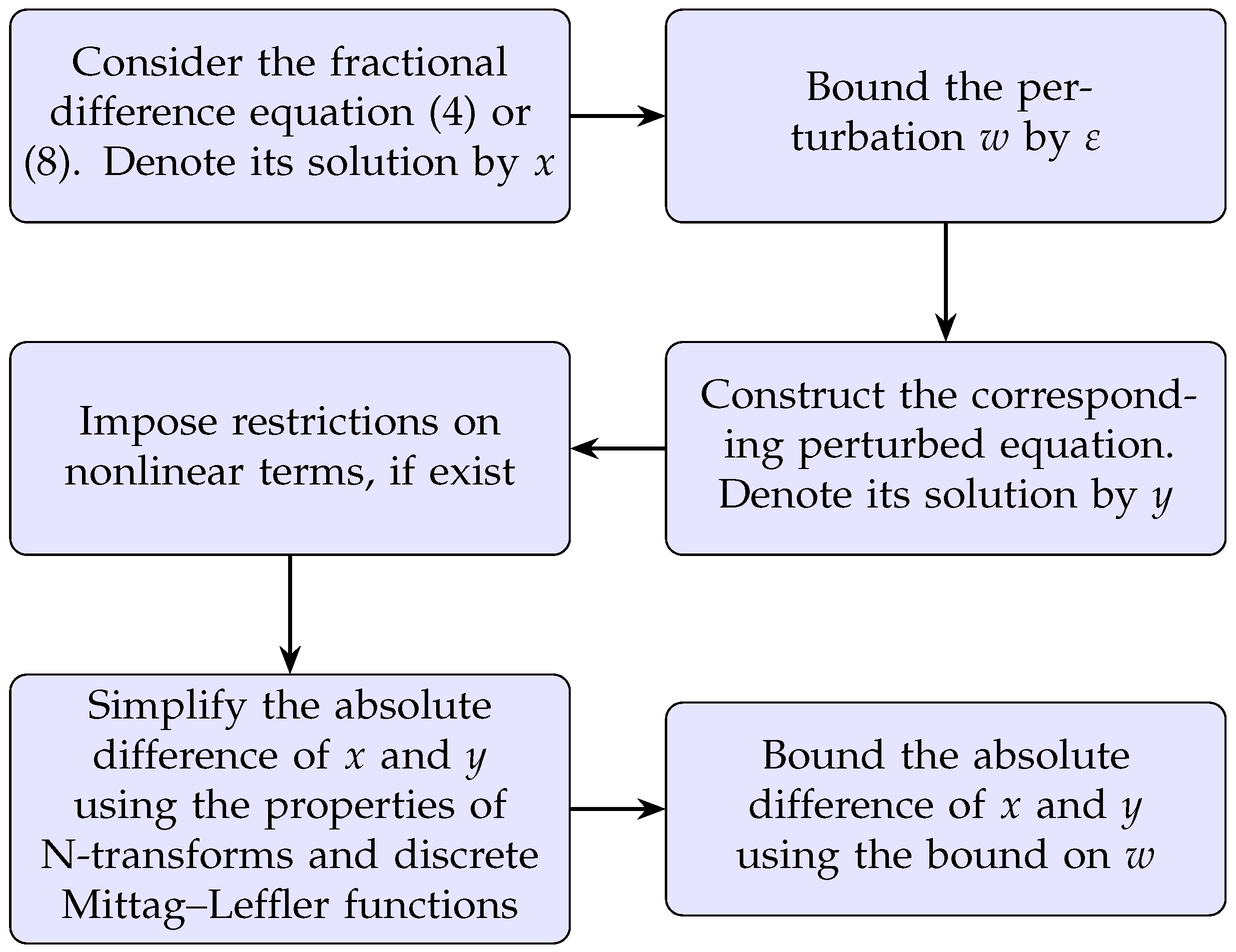
Our analysis is two-fold. First of all, we study the linear Hilfer nabla fractional difference equation and obtain its generalized Ulam–Hyers stability (consequently, Ulam–Hyers stability). As the second task, we investigate the sufficient conditions for the Ulam–Hyers stability of a neutral-type Hilfer nabla fractional difference equation with delay. Our methodology is summarized in Figure 1.

3.1. Linear Case

Consider the linear Hilfer fractional difference equation

$$\left({\nabla }_0^{\alpha ,\beta }x\right)\left(t\right)+\lambda x\left(t\right)=h\left(t\right),t\in {\mathbb{N}}_1,$$

(4)

where $0<\alpha \le 1,0\le \beta \le 1,\gamma =\alpha +\beta -\alpha \beta ,0<\lambda <1$ and $h:{\mathbb{N}}_1\to \mathbb{R}.$

Let $y:{\mathbb{N}}_0\to \mathbb{R}.$ Set

$$w\left(t\right):=\left({\nabla }_0^{\alpha ,\beta }y\right)\left(t\right)+\lambda y\left(t\right)-h\left(t\right),$$

(5)

for $t\in {\mathbb{N}}_1;$ then, we have

$$\begin{array}{cc}\hfill {\mathcal{N}}_1\left(w\left(t\right)\right)& ={\mathcal{N}}_1\left(\left({\nabla }_0^{\alpha ,\beta }y\right)\left(t\right)\right)+\lambda {\mathcal{N}}_1\left(y\left(t\right)\right)-{\mathcal{N}}_1\left(h\left(t\right)\right)\hfill \\ \hfill & =s^{\alpha }{\mathcal{N}}_0\left(y\left(t\right)\right)-{\displaystyle \frac{{\left(1-s\right)}^{-1}}{s^{\gamma -\alpha }}}y\left(0\right)+\lambda {\mathcal{N}}_0\left(y\left(t\right)\right)-\lambda {\left(1-s\right)}^{-1}y\left(0\right)\hfill \\ \hfill & -{\mathcal{N}}_0\left(h\left(t\right)\right)+{\displaystyle \frac{h\left(0\right)}{1-s}}\hfill \\ \hfill & =\left(s^{\alpha }+\lambda \right){\mathcal{N}}_0\left(y\left(t\right)\right)-\left({\displaystyle \frac{{\left(1-s\right)}^{-1}}{s^{\gamma -\alpha }}}+{\displaystyle \frac{\lambda }{1-s}}\right)y\left(0\right)-{\mathcal{N}}_0\left(h\left(t\right)\right)+{\displaystyle \frac{h\left(0\right)}{1-s}}\hfill \\ \hfill & =\left(s^{\alpha }+\lambda \right){\mathcal{N}}_0\left(y\left(t\right)\right)-{\displaystyle \frac{1}{1-s}}\left(s^{\alpha -\gamma }+\lambda \right)y\left(0\right)-{\mathcal{N}}_0\left(h\left(t\right)\right)+{\displaystyle \frac{h\left(0\right)}{1-s}}\hfill \\ \hfill & =\left(s^{\alpha }+\lambda \right){\mathcal{N}}_0\left(y\left(t\right)\right)-{\mathcal{N}}_0\left(h\left(t\right)\right)-{\displaystyle \frac{1}{1-s}}\left(\left(s^{\alpha -\gamma }+\lambda \right)y\left(0\right)-h\left(0\right)\right).\hfill \end{array}$$

This results in

$$\left(s^{\alpha }+\lambda \right){\mathcal{N}}_0\left(y\left(t\right)\right)={\mathcal{N}}_1\left(w\left(t\right)\right)+{\mathcal{N}}_0\left(h\left(t\right)\right)+{\displaystyle \frac{1}{1-s}}\left(\left(s^{\alpha -\gamma }+\lambda \right)y\left(0\right)-h\left(0\right)\right)$$

and

$${\mathcal{N}}_0\left(y\left(t\right)\right)={\left(s^{\alpha }+\lambda \right)}^{-1}\left({\mathcal{N}}_1\left(w\left(t\right)\right)+{\mathcal{N}}_0\left(h\left(t\right)\right)+{\displaystyle \frac{1}{1-s}}\left(\left(s^{\alpha -\gamma }+\lambda \right)y\left(0\right)-h\left(0\right)\right)\right).$$

(6)

Set

$$x\left(t\right):=\lambda y\left(0\right)E_{-\lambda ,\alpha ,\alpha -1}\left(t,\rho \left(0\right)\right)+y\left(0\right)E_{-\lambda ,\alpha ,\gamma -1}\left(t,\rho \left(0\right)\right)+{\displaystyle \sum _{s=1}^t}{E}_{-\lambda ,\alpha ,\alpha -1}\left(t,\rho \left(s\right)\right)h\left(s\right).$$

(7)

The Mittag-Leffler functions appearing in solution Formula (7) naturally arise from the inverse N-transform of the rational expressions encountered during the solution process. In particular, Lemma 3(ii) guarantees that the function $E_{-\lambda ,\alpha ,\alpha -1}(t,\rho \left(a\right))$ serves as an eigenfunction of the Hilfer fractional difference operator, which facilitates the derivation of a closed-form solution to the homogeneous part of the equation. Furthermore, Lemma 3(i) is utilized in the estimation of the perturbation accumulation term in the stability analysis, as seen in Equation (8), where the boundedness of the Mittag-Leffler function directly contributes to establishing the stability bound.

It is clear that $x\left(0\right)=y\left(0\right).$ Now, we apply the ${\mathcal{N}}_0$ transform to both sides of (7):

$$\begin{array}{cc}\hfill {\mathcal{N}}_0\left(x\left(t\right)\right)& =\left(\lambda y\left(0\right)-h\left(0\right)\right){\displaystyle \frac{1}{\left(1-s\right)\left(s^{\alpha }+\lambda \right)}}+y\left(0\right){\displaystyle \frac{s^{\alpha -\gamma }}{\left(1-s\right)\left(s^{\alpha }+\lambda \right)}}\hfill \\ \hfill & +{\mathcal{N}}_1\left(E_{-\lambda ,\alpha ,\alpha -1}\left(t,\rho \left(0\right)\right)\right){\mathcal{N}}_0\left(h\left(t\right)\right)\hfill \\ \hfill & =\left(\lambda y\left(0\right)-h\left(0\right)\right){\displaystyle \frac{1}{\left(1-s\right)\left(s^{\alpha }+\lambda \right)}}+y\left(0\right){\displaystyle \frac{s^{\alpha -\gamma }}{\left(1-s\right)\left(s^{\alpha }+\lambda \right)}}+{\displaystyle \frac{{\mathcal{N}}_0\left(h\left(t\right)\right)}{s^{\alpha }+\lambda }}.\hfill \end{array}$$

This implies

$$\left(s^{\alpha }+\lambda \right){\mathcal{N}}_0\left(x\left(t\right)\right)=\left(\lambda y\left(0\right)-h\left(0\right)\right){\displaystyle \frac{1}{1-s}}+y\left(0\right){\displaystyle \frac{s^{\alpha -\gamma }}{1-s}}+{\mathcal{N}}_0\left(h\left(t\right)\right)$$

and

$$\left(s^{\alpha }{\mathcal{N}}_0\left(x\left(t\right)\right)-{\displaystyle \frac{x\left(0\right)}{\left(1-s\right)s^{\gamma -\alpha }}}\right)+\lambda \left({\mathcal{N}}_0\left(x\left(t\right)\right)-{\displaystyle \frac{x\left(0\right)}{1-s}}\right)={\mathcal{N}}_0\left(h\left(t\right)\right)-{\displaystyle \frac{h\left(0\right)}{1-s}}.$$

Hence,

$${\mathcal{N}}_1\left(\left({\nabla }_0^{\alpha ,\beta }x\right)\left(t\right)\right)+\lambda {\mathcal{N}}_1\left(x\left(t\right)\right)={\mathcal{N}}_1\left(h\left(t\right)\right).$$

Since ${\mathcal{N}}_1$ transform is one to one, we get

$$\left({\nabla }_0^{\alpha ,\beta }x\right)\left(t\right)+\lambda x\left(t\right)=h\left(t\right)$$

and $(·)x$ given by (7) is a solution of (4).

Using (6) and (7), we get

$$\begin{array}{cc}\hfill {\mathcal{N}}_0\left(x\left(t\right)\right)-{\mathcal{N}}_0\left(y\left(t\right)\right)& =-{\left(s^{\alpha }+\lambda \right)}^{-1}{\mathcal{N}}_1\left(w\left(t\right)\right)\hfill \\ \hfill & ={\left(s^{\alpha }+\lambda \right)}^{-1}\left({\displaystyle \frac{w\left(0\right)}{1-s}}-{\mathcal{N}}_0\left(w\left(t\right)\right)\right)\hfill \\ \hfill & =w\left(0\right){\mathcal{N}}_0\left(E_{-\lambda ,\alpha ,\alpha -1}\left(t,\rho \left(0\right)\right)\right)-{\mathcal{N}}_1\left(E_{-\lambda ,\alpha ,\alpha -1}\left(t,0\right)\right){\mathcal{N}}_0\left(w\left(t\right)\right)\hfill \\ \hfill & =-{\mathcal{N}}_0\left({\displaystyle \sum _{s=1}^t}{E}_{-\lambda ,\alpha ,\alpha -1}\left(t,\rho \left(s\right)\right)w\left(s\right)\right).\hfill \end{array}$$

Since ${\mathcal{N}}_0$ is injective, it follows that

$$x\left(t\right)-y\left(t\right)=-{\displaystyle \sum _{s=1}^t}{E}_{-\lambda ,\alpha ,\alpha -1}\left(t,\rho \left(s\right)\right)w\left(s\right).$$

(8)

Now, we establish the following result regarding the generalized Ulam–Hyers stability:

Theorem 2. 

Let $y:{\mathbb{N}}_0\to \mathbb{R}$ and $\varphi :{\mathbb{N}}_0\to \left[0,\infty \right).$ If $\left|w\left(t\right)\right|\le \varphi \left(t\right)$ for $t\in {\mathbb{N}}_0,$ then there exists a solution $x:{\mathbb{N}}_0\to \mathbb{R}$ of (4) and $\psi :{\mathbb{N}}_0\to \left[0,\infty \right)$ such that

$$\left|x\left(t\right)-y\left(t\right)\right|\le \psi \left(t\right)\mathrm{for}\mathrm{all}t\in {\mathbb{N}}_0.$$

Proof. 

By (8), we write

$$\begin{array}{cc}\hfill \left|x\left(t\right)-y\left(t\right)\right|& \le {\displaystyle \sum _{s=1}^t}{E}_{-\lambda ,\alpha ,\alpha -1}\left(t,\rho \left(s\right)\right)\left|w\left(s\right)\right|\hfill \\ \hfill & \le {\displaystyle \sum _{s=1}^t}{E}_{-\lambda ,\alpha ,\alpha -1}\left(t,\rho \left(s\right)\right)\varphi \left(s\right).\hfill \end{array}$$

Note that ${lim}_{t\to \infty }{E}_{-\lambda ,\alpha ,\alpha -1}\left(t,\rho \left(s\right)\right)$ for $s=1,2,\cdots t$ converge to 0, and, therefore, there exists a finite real number $M>0$ such that $E_{-\lambda ,\alpha ,\alpha -1}\left(t,\rho \left(s\right)\right)\le M.$ Then, we get

$$\begin{array}{c}\hfill \left|x\left(t\right)-y\left(t\right)\right|\le M{\displaystyle \sum _{s=1}^t}\varphi \left(s\right)=\psi \left(t\right).\end{array}$$

This proves the assertion. □

By using the same method as that of the proof of Theorem 2, we obtain the following result:

Corollary 1. 

Let $y:{\mathbb{N}}_0\to \mathbb{R}$ and $\epsilon >0.$ If $\left|w\left(t\right)\right|\le \epsilon$ for $t\in {\mathbb{N}}_0,$ then there exists a solution $x:{\mathbb{N}}_0\to \mathbb{R}$ of (4) such that

$$\left|x\left(t\right)-y\left(t\right)\right|\le K\left(\epsilon \right)\mathrm{for}\mathrm{all}t\in {\mathbb{N}}_0.$$

3.2. Nonlinear Case

Let us consider the following neutral fractional delayed Hilfer difference equation:

$${\nabla }_0^{\alpha ,\beta }\left[x\left(t\right)-g\left(t,x\left(t-\tau \right)\right)\right]=f\left(t,x\left(t-\tau \right)\right),t\in {\mathbb{N}}_1^{\delta },$$

(9)

where $0<\alpha \le 1,0\le \beta \le 1$, $\gamma =\alpha +\beta -\alpha \beta ,$ $f,g:{\mathbb{N}}_1^{\delta }\times \mathbb{R}\to \mathbb{R},$ and ${\mathbb{N}}_1^{\delta }=1,2,\cdots ,\delta .$ By a solution of (9), we mean any function $x(·)$ satisfying (9) for all $t\in {\mathbb{N}}_0^{\delta }$ and the initial function $\xi \left(t\right)=x\left(t\right)$ for all $t\in \left[-\tau ,0\right]\cap \mathbb{Z}.$

Now, we present the following auxiliary result, which is crucial for the proof of our stability result:

Lemma 9 

([7]). The function $x(·)$ is a solution of (9) if and only if $x(·)$ satisfies

$$\begin{array}{cc}\hfill x\left(t\right)& =\left[\xi \left(0\right)-g\left(0,\xi \left(-\tau \right)\right)\right]H_{\gamma -1}\left(t,\rho \left(0\right)\right)+g\left(t,x\left(t-\tau \right)\right)\hfill \\ \hfill & +{\displaystyle \sum _{s=1}^t}{H}_{\alpha -1}\left(t,\rho \left(s\right)\right)f\left(s,x\left(s-\tau \right)\right).\hfill \end{array}$$

(10)

Next, we recall the following inequality:

$$\left|{\nabla }_0^{\alpha ,\beta }\left[x\left(t\right)-g\left(t,x\left(t-\tau \right)\right)\right]-f\left(t,x\left(t-\tau \right)\right)\right|\le \epsilon ,t\in {\mathbb{N}}_1^{\delta }.$$

(11)

Let the function $y(·)$ be a solution of (11), and let $x(·)$ be a solution of (9), which satisfies (10). Then, we set

$$\begin{array}{c}{\nabla }_0^{\alpha ,\beta }\left[x\left(t\right)-g\left(t,x\left(t-\tau \right)\right)\right]=f\left(t,x\left(t-\tau \right)\right),t\in {\mathbb{N}}_1^{\delta }\\ x\left(t\right)=y\left(t\right)=\xi \left(t\right)\mathrm{for}\mathrm{all}t\in \left[-\tau ,0\right]\cap \mathbb{Z}\end{array}.$$

Remark 1. 

The function $y(·)$ is a solution of (11) if and only if there exists a function $p:{\mathbb{N}}_0\to \mathbb{R}$ such that $\left|p\left(t\right)\right|\le \epsilon$ for $t\in {\mathbb{N}}_1^{\delta },$ and

$${\nabla }_0^{\alpha ,\beta }\left[x\left(t\right)-g\left(t,x\left(t-\tau \right)\right)\right]=f\left(t,x\left(t-\tau \right)\right)+p\left(t\right),t\in {\mathbb{N}}_1^{\delta }.$$

(12)

Remark 2. 

Suppose that $y(·)$ is a solution of (9). Then, a solution of

$${\nabla }_0^{\alpha ,\beta }\left[y\left(t\right)-g\left(t,y\left(t-\tau \right)\right)\right]=f\left(t,y\left(t-\tau \right)\right)+p\left(t\right),t\in {\mathbb{N}}_1^{\delta }$$

(13)

is given by

$$\begin{array}{cc}\hfill y\left(t\right)& =\left[\xi \left(0\right)-g\left(0,\xi \left(-\tau \right)\right)\right]H_{\gamma -1}\left(t,\rho \left(0\right)\right)+g\left(t,y\left(t-\tau \right)\right)\hfill \\ \hfill & +{\displaystyle \sum _{s=1}^t}{H}_{\alpha -1}\left(t,\rho \left(s\right)\right)\left(f\left(s,y\left(s-\tau \right)\right)+p\left(s\right)\right).\hfill \end{array}$$

This yields

$$\begin{array}{cc}\hfill & |y\left(t\right)-\left[\xi \left(0\right)-g\left(0,\xi \left(-\tau \right)\right)\right]H_{\gamma -1}\left(t,\rho \left(0\right)\right)\hfill \\ & -g\left(t,y\left(t-\tau \right)\right)-{\displaystyle \sum _{s=1}^t}{H}_{\alpha -1}\left(t,\rho \left(s\right)\right)f\left(s,y\left(s-\tau \right)\right)|\hfill \\ & =\left|{\displaystyle \sum _{s=1}^t}{H}_{\alpha -1}\left(t,\rho \left(s\right)\right)p\left(s\right)\right|\le \epsilon {\displaystyle \sum _{s=1}^t}{H}_{\alpha -1}\left(t,\rho \left(s\right)\right)=\epsilon H_{\alpha }\left(t,1\right)\le \epsilon H_{\alpha }\left(\delta ,1\right).\hfill \end{array}$$

Now, we are ready to present our stability result. Note that Equation (9) is said to be Ulam–Hyers stable if there exists a positive real number $K>0$ such that, for each $\epsilon >0$ and for each solution $y(·)$ of inequality (11), there exists a solution $x:{\mathbb{N}}_0^{\delta }\to \mathbb{R}$ of (9) such that

$$\left|x\left(t\right)-y\left(t\right)\right|\le K\epsilon ,t\in {\mathbb{N}}_0^{\delta }.$$

We have the following result:

Theorem 3. 

The delayed neutral Hilfer fractional difference Equation (9) is Ulam–Hyers stable if the following inequalities hold:

$$\begin{array}{cc}\hfill \left|f\left(t,\theta \right)-f\left(t,\kappa \right)\right|& \le W_1\left|\theta -\kappa \right|,\mathrm{for}{W}_1\ge 0\mathrm{and}t\in {\mathbb{N}}_0^{\delta }\hfill \end{array}$$

(14)

$$\begin{array}{cc}\hfill \left|g\left(t,\theta \right)-g\left(t,\kappa \right)\right|& \le W_2\left|\theta -\kappa \right|,\mathrm{for}{W}_2\in \left(0,1\right)\mathrm{and}t\in {\mathbb{N}}_0^{\delta }.\hfill \end{array}$$

(15)

Proof. 

Let $y(·)$ be as in (13) and $x(·)$ be a solution of (9). Taking into account (11), (14), and (15), we get

$$\begin{array}{cc}\hfill \left|y\left(t\right)-x\left(t\right)\right|& =\left|y\left(t\right)-\left[\xi \left(0\right)-g\left(0,\xi \left(-\tau \right)\right)\right]H_{\gamma -1}\left(t,\rho \left(0\right)\right)-g\left(t,x\left(t-\tau \right)\right)\right.\hfill \\ \hfill & \left.-{\displaystyle \sum _{s=1}^t}{H}_{\alpha -1}\left(t,\rho \left(s\right)\right)f\left(s,x\left(s-\tau \right)\right)\right|\hfill \\ \hfill & =\left|y\left(t\right)-\left[\xi \left(0\right)-g\left(0,\xi \left(-\tau \right)\right)\right]H_{\gamma -1}\left(t,\rho \left(0\right)\right)-g\left(t,y\left(t-\tau \right)\right)\right.\hfill \\ \hfill & +g\left(t,y\left(t-\tau \right)\right)-g\left(t,x\left(t-\tau \right)\right)-{\displaystyle \sum _{s=1}^t}{H}_{\alpha -1}\left(t,\rho \left(s\right)\right)f\left(s,y\left(s-\tau \right)\right)\hfill \\ \hfill & \left.+{\displaystyle \sum _{s=1}^t}{H}_{\alpha -1}\left(t,\rho \left(s\right)\right)\left(f\left(s,y\left(s-\tau \right)\right)-f\left(s,x\left(s-\tau \right)\right)\right)\right|\hfill \\ \hfill & \le \left|y\left(t\right)-\left[\xi \left(0\right)-g\left(0,\xi \left(-\tau \right)\right)\right]H_{\gamma -1}\left(t,\rho \left(0\right)\right)\right.\hfill \\ \hfill & \left.-g\left(t,y\left(t-\tau \right)\right)-{\displaystyle \sum _{s=1}^t}{H}_{\alpha -1}\left(t,\rho \left(s\right)\right)f\left(s,y\left(s-\tau \right)\right)\right|\hfill \\ \hfill & +\left|g\left(t,y\left(t-\tau \right)\right)-g\left(t,x\left(t-\tau \right)\right)\right|\hfill \\ \hfill & +{\displaystyle \sum _{s=1}^t}{H}_{\alpha -1}\left(t,\rho \left(s\right)\right)\left|f\left(s,y\left(s-\tau \right)\right)-f\left(s,x\left(s-\tau \right)\right)\right|,\hfill \end{array}$$

and this results in

$$\left|y-x\right|\le \epsilon H_{\alpha }\left(\delta ,1\right)+W_2\left|y-x\right|+W_1{\displaystyle \sum _{s=1}^t}{H}_{\alpha -1}\left(t,\rho \left(s\right)\right)\left|y-x\right|.$$

Therefore,

$$\left|y-x\right|\le {\displaystyle \frac{\epsilon }{1-W_2}}{H}_{\alpha }\left(\delta ,1\right)+{\displaystyle \frac{W_1}{1-W_2}}{\displaystyle \sum _{s=1}^t}{H}_{\alpha -1}\left(t,\rho \left(s\right)\right).$$

Now, Theorem 1 gives

$$\begin{array}{c}\hfill \left|y-x\right|\le {\displaystyle \frac{\epsilon }{1-W_2}}{H}_{\alpha }\left(\delta ,1\right)E_{{\displaystyle \frac{W_1}{1-W_2}},\alpha ,0}\left(t,0\right)\le {\displaystyle \frac{\epsilon }{1-W_2}}{H}_{\alpha }\left(\delta ,1\right)E_{{\displaystyle \frac{W_1}{1-W_2}},\alpha ,0}\left(\delta ,0\right)\le K\epsilon ,\end{array}$$

which completes the proof. □

Remark 3. 

In Theorem 3, the stability constant K is given by

$$K(\alpha ,\delta ,W_1,W_2)={\displaystyle \frac{1}{1-W_2}}·H_{\alpha }(\delta ,1)·E_{{\displaystyle \frac{W_1}{1-W_2}},\alpha ,0}(\delta ,0),$$

where $H_{\alpha }(\delta ,1)={\displaystyle \frac{{(\delta -1)}^{\alpha -1}}{\mathsf{\Gamma }\left(\alpha \right)}}$ and $E_{a,\alpha ,0}(·)$ is the three-parameter Mittag-Leffler function.

To illustrate this dependence, we fix $W_1=1$ and $W_2=0.8$ and visualize K as a function of the fractional order $\alpha \in (0.1,1]$ and time horizon $\delta \in \{1,2,\dots ,10\}$. The resulting surface plot is shown in Figure 2.

As expected, the stability constant increases with an increasing δ, indicating higher sensitivity to perturbations over longer horizons. The variation with α reflects the memory effect inherent in fractional-order systems, where a smaller α may amplify the influence of earlier states.

Remark 4 

(On Limiting Cases $\beta =0$ and $\beta =1$). As stated in Definition 3, the Hilfer nabla fractional difference operator reduces to the Riemann–Liouville type when $\beta =0$ and to the Caputo type when $\beta =1$. From Equation (8), we observe that the right-hand side is independent of β, which implies that the form of the stability estimate in Theorem 2 and Corollary 1 remains valid for both limiting cases.

On the other hand, for the nonlinear delayed neutral case, parameter β significantly influences the structure of the solution due to its impact on the initial conditions and memory weights. If we mimic the proof of Theorem 3 by setting $\beta =0$ and $\beta =1$, the corresponding values of the stability constant K become

$$K_0={\displaystyle \frac{1}{1-W_2}}·H_{\alpha }(\delta ,1)·E_{{\displaystyle \frac{W_1}{1-W_2}},\alpha ,0}(\delta ,0)\mathrm{with}\gamma =\alpha ,$$

$$K_1={\displaystyle \frac{1}{1-W_2}}·H_{\alpha }(\delta ,1)·E_{{\displaystyle \frac{W_1}{1-W_2}},\alpha ,0}(\delta ,0)\mathrm{with}\gamma =1.$$

Although the expression of K appears to be formally similar, the change in the value of $\gamma =\alpha +\beta -\alpha \beta$ affects the solution representation (see Lemma 7) and can lead to different stability behaviors depending on the sensitivity of $E_{p,\alpha ,0}$ to the order and initial data.

This observation highlights that parameter β plays a non-trivial role in the dynamics of delayed neutral Hilfer fractional difference equations, especially in how the initial history affects the long-term stability. Including the limiting cases ensures completeness and clarity for readers who may be more familiar with the classical Riemann–Liouville or Caputo settings.

4. Examples

In this section, we provide a summary and several illustrative applications of our results. As shown in

Table 1. Comparison of original and perturbed equations with stability results.

S. No.	Original Eq.	Perturbed Eq.	Bound on Perturbation	Bound on $\left|\mathit{x}\right(\mathit{t})-\mathit{y}(\mathit{t}\left)\right|$ and Stability
1	(4)	(5)	$\varphi \left(t\right)$	$\psi \left(t\right)$ — Theorem 2: Generalized Ulam–Hyers Stability of (4)
2	(4)	(5)	$\epsilon$	$K\left(\epsilon \right)$ — Corollary 1: Ulam–Hyers Stability of (4)
3	(9)	(11)	$\epsilon$	$K\epsilon$ — Theorem 3: Ulam–Hyers Stability of (9)

, the bounds on the absolute difference vary depending on the form of the perturbation.

Example 1. 

Consider (9) with $\alpha =0.5$, $\beta =0.5$, $\tau =3$, $\delta =5$,

$$g(t,\xi )={\displaystyle \frac{H_{0.25}(t,0)\xi }{2}},\mathit{and}f(t,\xi )=H_{0.75}(t,0)+sin\xi ,\mathit{for}\mathit{all}(t,\xi )\in {\mathbb{N}}_0^{\delta }\times \mathbb{R}.$$

Consider

$$\begin{array}{cc}\hfill \left|g\left(t,x_1\right)-g\left(t,x_2\right)\right|& ={\displaystyle \frac{H_{0.25}(t,0)}{2}}\left|x_1-x_2\right|\hfill \\ \hfill & \le {\displaystyle \frac{H_{0.25}(5,0)}{2}}\left|x_1-x_2\right|\hfill \\ \hfill & =W_2\left|x_1-x_2\right|,\hfill \end{array}$$

for all $(t,\xi )\in {\mathbb{N}}_0^{\delta }\times \mathbb{R}$ implying that (15) holds with $W_2={\displaystyle \frac{H_{0.25}(5,0)}{2}}\approx 0.8094\in (0,1)$. Also,

$$\begin{array}{cc}\hfill \left|f\left(t,x_1\right)-f\left(t,x_2\right)\right|& \le \left|x_1-x_2\right|\hfill \\ \hfill & =W_1\left|x_1-x_2\right|,\hfill \end{array}$$

for all $(t,\xi )\in {\mathbb{N}}_0^{\delta }\times \mathbb{R}$ implying that (14) holds with $W_1=1>0$. Thus, all assumptions of Theorem 3 hold. Therefore, (9) is Ulam–Hyers stable.

To further support the analytical findings presented in Example 1, we provide a numerical simulation that visualizes the behavior of the solutions. Specifically, we numerically compute the solution $x\left(t\right)$ of the fractional difference equation under consideration using the recursive formulation in Equation (9), with $\alpha =0.5$, $\beta =0.5$, $\tau =3$, and $\delta =5$. We consider an initial function $\xi \left(t\right)$ defined on $[-\tau ,0]$, and we generate a perturbed solution $y\left(t\right)$ by adding small bounded noise to $\xi \left(t\right)$.

Figure 3 displays the evolution of both $x\left(t\right)$ and $y\left(t\right)$, and Figure 4 shows the corresponding error $\left|x\right(t)-y(t\left)\right|$. These results visually confirm the theoretical prediction of Ulam–Hyers stability: the deviation remains bounded for all $t\in [0,\delta ]$.

Example 2. 

Consider Equation (9) with $\alpha =0.5$, $\beta =0.5$, $\tau =3$, $\delta =5$,

$$g(t,\xi )={\displaystyle \frac{H_{0.25}(t,0)\xi }{2}}\mathit{and}f(t,\xi )=H_{0.75}(t,0)+sin\xi \mathit{for}\mathit{all}(t,\xi )\in {\mathbb{N}}_0^{\delta }\times \mathbb{R}.$$

Then,

$$\begin{array}{c}\hfill \left|g\left(t,x_1\right)-g\left(t,x_2\right)\right|={\displaystyle \frac{H_{0.25}(t,0)}{2}}\left|x_1-x_2\right|\le {\displaystyle \frac{H_{0.25}(5,0)}{2}}\left|x_1-x_2\right|=W_2\left|x_1-x_2\right|,\end{array}$$

for all $(t,\xi )\in {\mathbb{N}}_0^{\delta }\times \mathbb{R}$ implying that (15) holds with $W_2={\displaystyle \frac{H_{0.25}(5,0)}{2}}\approx 0.8094\in (0,1)$. Also,

$$\begin{array}{c}\hfill \left|f\left(t,x_1\right)-f\left(t,x_2\right)\right|\le \left|x_1-x_2\right|=W_1\left|x_1-x_2\right|,\end{array}$$

for all $(t,\xi )\in {\mathbb{N}}_0^{\delta }\times \mathbb{R}$ implying that (14) holds with $W_1=1>0$. Thus, all assumptions of Theorem 3 hold. Therefore, (9) is Ulam–Hyers stable.

To complement the analytical results in Example 2, we provide numerical simulations illustrating the Ulam–Hyers stability of the delayed nonlinear Hilfer fractional difference equation. Using the recursive formulation in Equation (9), we compute the solution $x\left(t\right)$ for $t\in [0,5]$ with a chosen initial function $\xi \left(t\right)$. A perturbed solution $y\left(t\right)$ is then generated by adding small noise to $\xi \left(t\right)$ and solving Equation (12). Figure 5 compares the true and perturbed solutions, while Figure 6 displays the deviation $\left|x\right(t)-y(t\left)\right|$. The results confirm that the error remains bounded throughout the interval, validating the Ulam–Hyers stability established in Theorem 3.

5. Concluding Remarks

In the present work, we studied the Ulam–Hyers stability of linear and nonlinear neutral fractional difference equations involving nabla differences and investigated the sufficient conditions providing Ulam–Hyers stability. In the nonlinear case, we particularly focused on the neutral Hilfer fractional difference equations for which, to the best of our knowledge, Ulam–Hyers stability has not been taken into account in the existing literature. We should highlight that the Ulam–Hyers stability of the nonlinear fractional difference equations with Hilfer nabla differences

$$\left({\nabla }^{\alpha ,\beta }x\right)\left(t\right)=f\left(t,x\left(t-\tau \right)\right)$$

(16)

has already been studied in [6,11]. From our mathematical point of view, it may be an interesting task to investigate the Ulam–Hyers stability of the semi-linear fractional Hilfer difference equations

$$\left({\nabla }^{\alpha ,\beta }x\right)\left(t\right)+\lambda x\left(t\right)=f\left(t,x\left(t-\tau \right)\right)$$

(17)

which generalize Equation (16), and the results in the above-mentioned references. Since the stability analysis of Equation (17) can be constructed with arguments similar to those given in Section 3.2, we leave this task to the readers. Since we are working on a discrete domain, the expressions of solutions, and the absolute differences of solutions, we are examining whether the terms provide a numerical scheme when they are suitably rearranged.