Football Games Consist of a Self-Similar Sequence of Ball-Keeping Durations


Abstract
1. Introduction
2. Methods
2.1. Dataset
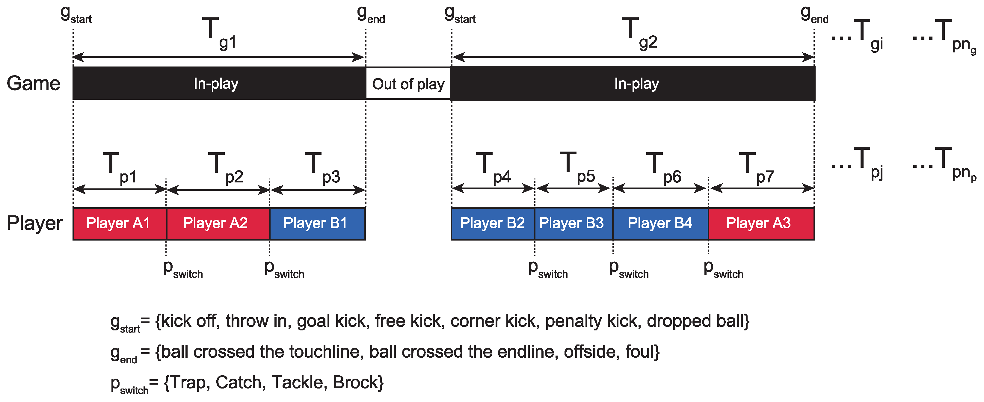
2.2. Definition of Variables
2.3. Power-Law Fitting
3. Results
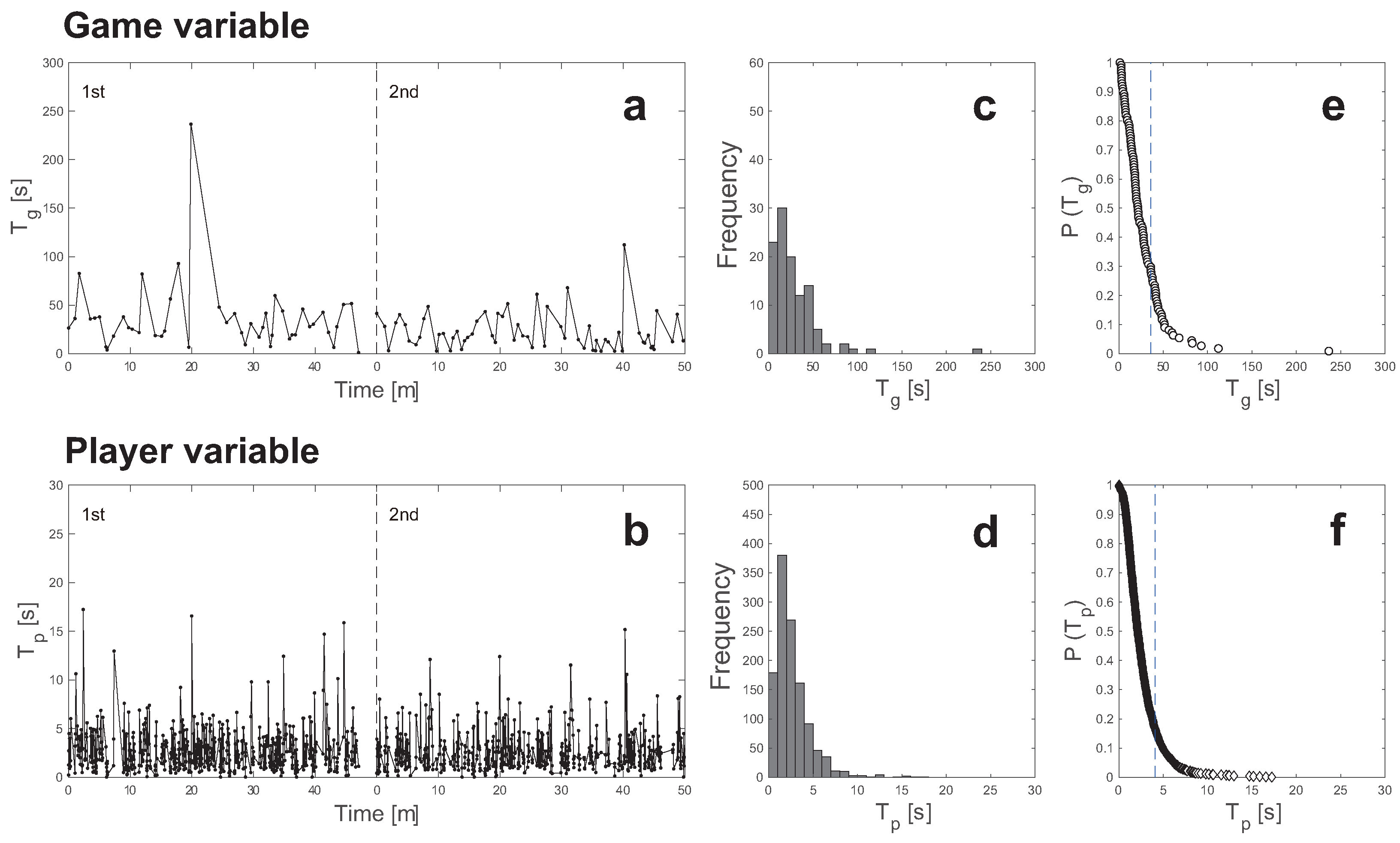
3.1. Time-Series Graphs of and
3.2. Histogram and CDF Curves
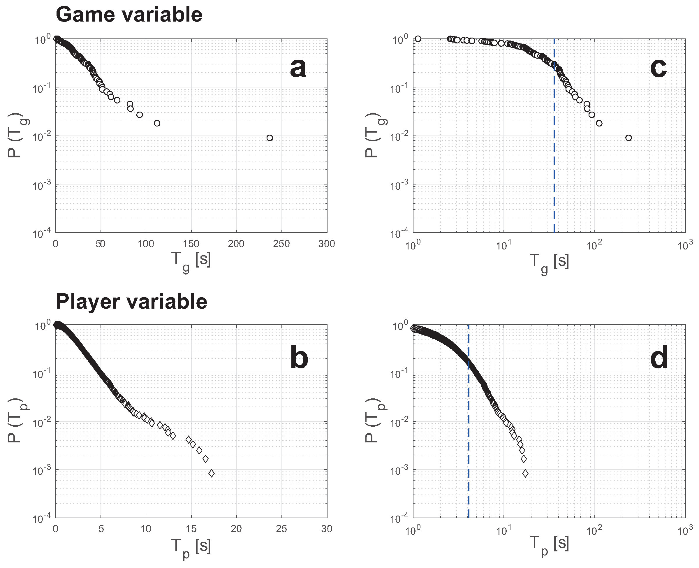
3.3. Exponential Distribution and Power-Law Distribution
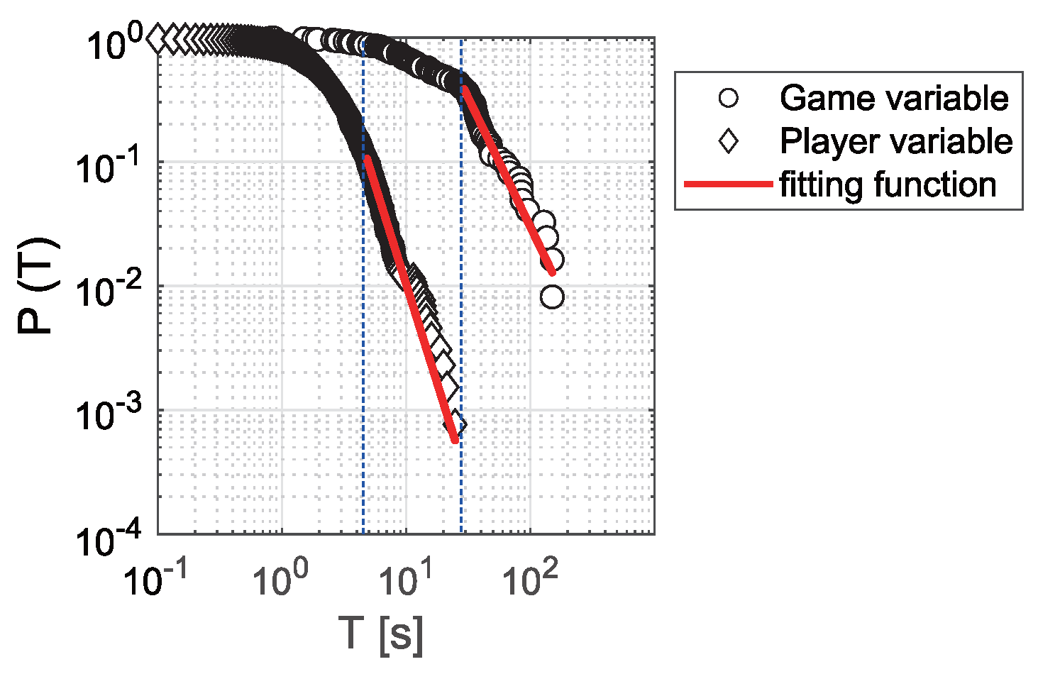
3.4. Transition of the Power-Law Range Between and
4. Discussion
5. Conclusions
Supplementary Materials
Author Contributions
Funding
Institutional Review Board Statement
Informed Consent Statement
Data Availability Statement
Conflicts of Interest
References
- Ramos, J.P.; Lopes, R.J.; Araújo, D. Interactions between soccer teams reveal both design and emergence: Cooperation, competition and Zipf-Mandelbrot regularity. Chaos Solitons Fract. 2020, 137, 109872. [Google Scholar] [CrossRef]
- Kijima, A.; Yokoyama, K.; Shima, H.; Yamamoto, Y. Emergence of self-similarity in football dynamics. Eur. Phys. J. B 2014, 87, 41. [Google Scholar] [CrossRef]
- Bueno, M.J.O.; Silva, M.; Cunha, S.A.; Torres, R.D.S.; Moura, F.A. Multiscale fractal dimension applied to tactical analysis in football: A novel approach to evaluate the shapes of team organization on the pitch. PLoS ONE 2021, 16, e0256771. [Google Scholar] [CrossRef] [PubMed]
- Yamamoto, Y.; Yokoyama, K. Common and unique network dynamics in football games. PLoS ONE 2011, 6, e29638. [Google Scholar] [CrossRef] [PubMed]
- Moura, F.A.; Bueno, M.J.d.O.; Caetano, F.G.; Silva, M.; Cunha, S.A.; Torres, R.d.S. Exploring the recurrent states of football teams’ tactical organization on the pitch during Brazilian official matches. PLoS ONE 2024, 19, e0308320. [Google Scholar] [CrossRef] [PubMed]
- Lames, M.; Hermann, S.; Prüßner, R.; Meth, H. Football match dynamics explored by recurrence analysis. Front. Psychol. 2021, 12, 747058. [Google Scholar] [CrossRef] [PubMed]
- Welch, M.; Schaerf, T.M.; Murphy, A. Collective states and their transitions in football. PLoS ONE 2021, 16, e0251970. [Google Scholar] [CrossRef] [PubMed]
- Ribeiro, J.; Davids, K.; Araújo, D.; Guilherme, J.; Silva, P.; Garganta, J. Exploiting bi-directional self-organizing tendencies in team sports: The role of the game model and tactical principles of play. Front. Psychol. 2019, 10, 2213. [Google Scholar] [CrossRef] [PubMed]
- Clauset, A.; Shalizi, C.R.; Newman, M.E.J. Power-law distributions in empirical data. SIAM Rev. 2009, 51, 661–703. [Google Scholar] [CrossRef]
- Lo, C.C.; Chou, T.; Penzel, T.; Scammell, T.E.; Strecker, R.E.; Stanley, H.E.; Ivanov, P.C. Common scale-invariant patterns of sleep–wake transitions across mammalian species. Proc. Natl. Acad. Sci. USA 2004, 101, 17545–17548. [Google Scholar] [CrossRef] [PubMed]
- Xavier, G. Zipf’s law for cities: An explanation. Q. J. Econ. 1999, 114, 739–767. [Google Scholar]
- Akiba, Y.; Wang, S.; Sato, M.; Shima, H. Impact of land-use differences on block-size distribution in Tokyo. J. Phys. Soc. Jpn. 2023, 92, 104801. [Google Scholar] [CrossRef]
- Clauset, A.; Young, M.; Gleditsch, K.S. On the frequency of severe terrorist events. J. Confl. Resolut. 2007, 51, 58–87. [Google Scholar] [CrossRef]
- Mandelbrot, B.B.; Hudson, R.L. The (Mis)behavior of Markets: A Fractal View of Risk, Ruin, and Reward; Basic Books: New York, NY, USA, 2004. [Google Scholar]
- Da Silva, S.; Matsushita, R.; Silveira, E. Hidden power law patterns in the top European football leagues. Phys. A Stat. Mech. Appl. 2013, 392, 5376–5386. [Google Scholar] [CrossRef]
- Barábasi, A.L. The origin of bursts and heavy tails in human dynamics. Nature 2005, 435, 207–211. [Google Scholar] [CrossRef] [PubMed]
- Oliveira, J.; Barabási, A.L. Darwin and Einstein correspondence patterns. Nature 2005, 437, 1251. [Google Scholar] [CrossRef] [PubMed]
- Roebber, P.J.; Burlingame, B.M.; deWinter, A. On the existence of momentum in professional football. PLoS ONE 2022, 17, e0269604. [Google Scholar] [CrossRef]
- Feldman, R.M.; Valdez-Flores, C. Applied Probability and Stochastic Processes; Springer: Berlin/Heildelberg, Germany, 2010; Volume 2. [Google Scholar]
- Sneyd, J.; Fewster, R.M.; McGillivray, D. Common continuous probability models. In Mathematics and Statistics for Science; Springer International Publishing: Cham, Switzerland, 2022; pp. 829–865. [Google Scholar]
- Beggs, C. Soccer Analytics: An Introduction Using R; CRC Press: Boca Raton, FL, USA, 2024. [Google Scholar]

| Match No. | Observed Number | Lower Bound | Exponent | Analyzed Number | p-Value | |||||
|---|---|---|---|---|---|---|---|---|---|---|
| 1 | 123 | 1311 | 29.3 | 4.8 | 3.08 | 4.19 | 47 | 138 | 0.44 | 0.32 |
| 2 | 112 | 1317 | 18.9 | 4.4 | 2.30 | 4.54 | 57 | 161 | 0.07 | 0.56 |
| 3 | 120 | 1246 | 39.9 | 3.5 | 3.32 | 3.54 | 26 | 254 | 0.85 | 0.78 |
| 4 | 108 | 1258 | 9.4 | 5.0 | 1.93 | 3.81 | 83 | 86 | 0.00 | 0.93 |
| 5 | 95 | 1369 | 39.7 | 4.1 | 2.63 | 4.22 | 34 | 235 | 0.00 | 0.13 |
| 6 | 126 | 1052 | 37.2 | 3.3 | 3.18 | 3.46 | 22 | 267 | 0.42 | 0.03 |
| 7 | 101 | 1342 | 67.9 | 4.4 | 4.44 | 4.36 | 19 | 176 | 0.23 | 0.35 |
| 8 | 81 | 1286 | 66.4 | 5.0 | 3.52 | 5.20 | 20 | 146 | 0.90 | 0.59 |
| 9 | 114 | 1005 | 30.8 | 3.0 | 3.10 | 3.41 | 35 | 284 | 0.26 | 0.38 |
| 10 | 111 | 1199 | 35.9 | 4.1 | 3.80 | 4.02 | 33 | 201 | 0.85 | 0.16 |
| Mean | 109.1 | 1238.5 | 43.9 | 4.2 | 3.4 | 4.1 | 28.9 | 186.8 | ||
| SD | 13.70 | 121.44 | 16.29 | 0.67 | 0.49 | 0.54 | 10.1 | 62.7 | ||
Disclaimer/Publisher’s Note: The statements, opinions and data contained in all publications are solely those of the individual author(s) and contributor(s) and not of MDPI and/or the editor(s). MDPI and/or the editor(s) disclaim responsibility for any injury to people or property resulting from any ideas, methods, instructions or products referred to in the content. |
© 2025 by the authors. Licensee MDPI, Basel, Switzerland. This article is an open access article distributed under the terms and conditions of the Creative Commons Attribution (CC BY) license (https://creativecommons.org/licenses/by/4.0/).
Share and Cite
Yokoyama, K.; Shima, H.; Kijima, A.; Yamamoto, Y. Football Games Consist of a Self-Similar Sequence of Ball-Keeping Durations. Fractal Fract. 2025, 9, 406. https://doi.org/10.3390/fractalfract9070406
Yokoyama K, Shima H, Kijima A, Yamamoto Y. Football Games Consist of a Self-Similar Sequence of Ball-Keeping Durations. Fractal and Fractional. 2025; 9(7):406. https://doi.org/10.3390/fractalfract9070406
Chicago/Turabian StyleYokoyama, Keiko, Hiroyuki Shima, Akifumi Kijima, and Yuji Yamamoto. 2025. "Football Games Consist of a Self-Similar Sequence of Ball-Keeping Durations" Fractal and Fractional 9, no. 7: 406. https://doi.org/10.3390/fractalfract9070406
APA StyleYokoyama, K., Shima, H., Kijima, A., & Yamamoto, Y. (2025). Football Games Consist of a Self-Similar Sequence of Ball-Keeping Durations. Fractal and Fractional, 9(7), 406. https://doi.org/10.3390/fractalfract9070406