On Computation of Prefactor of Free Boundary in One Dimensional One-Phase Fractional Stefan Problems

Abstract

We consider the melting of a one-dimensional domain ($x\ge 0$), initially at the melting temperature $u=0$, by fixing the boundary temperature to a value $u(0,t)=U_0>0$—the so called Stefan melting problem. The governing transient heat-conduction equation involves a time derivative and the spatial derivative of the temperature gradient. In the general case the order of the time derivative and the gradient can take values in the range $(0,1]$. In these problems it is known that the advance of the melt front $s\left(t\right)$ can be uniquely determined by a specified prefactor multiplying a power of time related to the order of the fractional derivatives in the governing equation. For given fractional orders the value of the prefactor is the unique solution to a transcendental equation formed in terms of special functions. Here, our main purpose is to provide efficient numerical schemes with low computational complexity to compute these prefactors. The values of the prefactors are obtained through a dimensionalization that allows the recovery of the solution for the quasi-stationary case when the Stefan number approaches zero. The mathematical analysis of this convergence is given and provides consistency to the numerical results obtained.

1. Introduction

The Stefan problem of melting is a well-known free boundary problem that has been deeply studied in the last century. The scope of this model is very broad, as can be seen in the review article [1], which cites and compiles more than 5000 articles on Stefan problems up to the year 2000.

When we deal with one-dimensional Stefan problems, under certain initial and boundary conditions, the motion of the free boundary (the melt front) behaves as the square of time t [2,3]. In particular, if we address the one-phase Stefan problem with a constant boundary condition, that is, if we consider the problem to find the pair of functions $\{u,s\}$ representing the temperature and the advance of the interface, such that

$$\begin{array}{ccc}\left(i\right)\hfill & \rho c{u}_t(x,t)=k{u}_{xx}(x,t)\hfill & 0<x<s\left(t\right),0<t<T,\hfill \\ \left(ii\right)\hfill & u(0,t)=U_0>0\hfill & 0<t<T,\hfill \\ \left(iii\right)\hfill & u\left(s\right(t),t)=0\hfill & 0<t<T,\hfill \\ \left(iv\right)\hfill & s\left(0\right)=0,\hfill & \\ \left(v\right)\hfill & \rho \mathsf{\ell }\dot{s}\left(t\right)=-\underset{x\to s{\left(t\right)}^{-}}{lim}k{u}_x(x,t)\hfill & 0<t<T,\hfill \end{array}$$

(1)

then the free boundary is given in terms of the square root of time,

$$s\left(t\right)=\theta \lambda \sqrt{t},t\ge 0,{\lambda }^2={\displaystyle \frac{k}{\rho c}},$$

(2)

where $\theta$ is the positive solution to the transcendental equation

$${\displaystyle \frac{x}{2}}erf\left({\displaystyle \frac{x}{2}}\right)e^{x^2/4}={\displaystyle \frac{Ste}{\sqrt{\pi }}},$$

(3)

and $Ste$ is the dimensionless Stefan number (see

Table 1. Nomenclature table with property dimensions: [M] mass, [T] time, [L] length, and [K] temperature.

Symbol	Definition	Dimension
u	Temperature	[K]
x	Spatial position	[L]
t	time	[T]
k	thermal conductivity	$\left[{\displaystyle \frac{\mathrm{ML}}{{\mathrm{KT}}^3}}\right]$
$\rho$	mass density	$\left[{\displaystyle \frac{\mathrm{M}}{{\mathrm{L}}^3}}\right]$
c	specific heat	$\left[{\displaystyle \frac{{\mathrm{L}}^2}{{\mathrm{KT}}^2}}\right]$
${\lambda }^2={\displaystyle \frac{k}{\rho c}}$	diffusion coefficient	$\left[{\displaystyle \frac{{\mathrm{L}}^2}{\mathrm{T}}}\right]$
ℓ	latent heat per unit mass	$\left[{\displaystyle \frac{{\mathrm{L}}^2}{{\mathrm{T}}^2}}\right]$
$\mathrm{Ste}={\displaystyle \frac{U_{0}c}{\mathsf{\ell }}}$	Stefan number	[-]

). We call $\theta$ the prefactor of the free boundary because, clearly, the advance of the interface is totally characterized by this number. The relevance of computing this parameter (which is relatively easy nowadays) was revealed by Solomon in [4] by giving exact data and demonstrating the importance of similarity solutions in semi-infinite domains to approximate exact solutions.

The heat transport governing equation in the Stefan problem above, (1)-$\left(i\right)$, is the classical diffusion equation. This equation arises as a consequence of inserting the phenomenological Fourier law for heat transfer into the heat continuity equation (first law of thermodynamics). However, the Fourier law is not the only way to model heat transfer. The theory of non-Fourier heat transfer is highly diverse, as can be observed, for instance, in Zhmakin’s book [5] or the works [6,7,8,9,10]. Such treatments are suitable for modeling heat transfer in the presence of fractal structures or amorphous materials like glassy polymers [11] or silica glasses [12]. The focus of this article is a particular class of non-Fourier heat transfer models, namely those that employ fractional calculus to describe anomalous diffusion [13]. More explicitly, we consider here non-Fourier models in the presence of fractional integrals or derivatives of Riemann–Liouville or Caputo type. We refer the readers to the works of Metzler and Klafter [14] and Voller [15], which provide an in-depth discussion on the modeling of anomalous diffusion processes using fractional derivatives, as well as the books [16,17,18,19,20] for the theory and applications of fractional diffusion equations.

When the presence of anomalous diffusion is considered in a free boundary problem with an imposed constant temperature at the fixed boundary, an interesting feature emerges: the advance of the free boundary is proportional to a power of t that differs from $1/2$ (see, e.g., [21] or [22]). That is,

$$s_{\alpha }\left(t\right)={\theta }_{\alpha }{\lambda }_{\alpha }{t}^{\gamma \left(\alpha \right)},t\ge 0;$$

(4)

${\lambda }_{\alpha }$ is an “extended” diffusivity, which will be clarified later. When $\gamma \left(\alpha \right)>1/2$ the process is referred to as superdiffusive and when $\gamma \left(\alpha \right)<1/2$, it is referred to as subdiffusive.

From Equation (4) we can deduce that, in the subdiffusive case, the front initially progresses rapidly but begins to slow down after a certain point in time. In contrast, the superdiffusive case starts more slowly, eventually surpassing the diffusive case abruptly at later times.

Our primary interest lies in determining the exact position of the front at any given time. To achieve this, it is essential to compute the value of the prefactor.

We are strongly convinced that fractional models can be valuable when studying the evolution of the free boundary. Thus, in mirroring classical work on Stefan problems [4], our goal here is to develop algorithms and techniques to compute the prefactor ${\theta }_{\alpha }$ associated with both super- and sub-diffusive one-dimensional, one-phase Stefan melting problems. In carrying out this task, we will use the similarity solutions of anomalous Stefan problems, which have been previously presented in the literature. In this light, we emphasize that the key component in our work is to arrive at computations that produce explicit numerical values for the prefactors ${\theta }_{\alpha }$. Beyond their intrinsic value, such results are useful in validating the effectiveness and accuracy of numerical methods for phase-change problems in the presence of anomalous diffusion, e.g., [23,24,25,26]. As a verification of our proposed computations, we provide a mathematical analysis that shows that when the governing dimensionless group, the Stefan number, satisfies $Ste\to 0$, our calculations for ${\theta }_{\alpha }$ converge to the known explicit values associated with quasi-stationary anomalous Stefan problems [21,22].

Our paper is laid out as follows. In Section 2, the time fractional and space fractional Stefan problems for a melting process are presented. Section 3 is devoted to the dimensionless scaling of such problems, highlighting the role of the Stefan number in each case. Section 4 and Section 5 deal with the space fractional and time fractional cases, respectively, which both have the same structure. The self-similar solutions for the general and the stationary problems are presented first. Then, a method for the computation of the prefactor is presented, and finally, an analytical proof of the convergence of the prefactors of the general solutions to the prefactors of the quasi-stationary solution when the Stefan number $Ste$ approaches zero is given. Section 6 is devoted to providing a bridge between the mathematical results and the verification of numerical methods. Here, we carefully spell out the physical nature of Stefan problems in fractional space and time domains. Finally, we present the conclusions and future work in Section 7.

2. Modeling the Space and Time Fractional Stefan Problems in a Melting Process

The modeling and justification of fractional free boundary problems is an active area of research. While these problems were initially studied by simply replacing classical derivatives with fractional ones in traditional models [27], there is now growing evidence that fractional phase-change models can be derived from first physical principles. This is supported by the theory of anomalous diffusion and its relationship to non-Fourier heat fluxes.

In this work, we present a formal derivation of such models using the thermal continuity equations. For readers interested in the physical derivation of these models and their application in describing heat transfer problems in heterogeneous media, we refer to [15,21] and the references therein.

Now, suppose that $\mathsf{\Omega }$ is a cylinder of anomalous phase change material with constant cross-section A and length $[0,l]$, where $l>>1$ is an isolated extreme. Let $u=u(x,t)$ be the temperature of the cylinder at position x and time t and let $q=q(x,t)$ be the heat flux. We assume that, initially, the bar is at its melt temperature $u=U_m$ and a melting process with a sharp moving interface $s=s\left(t\right)$ is initiated by imposing a constant temperature $U_0>U_m$ at $x=0$. This free boundary, representing the moving melt interface, is assumed to be an increasing function in time, i.e,

$$x=s\left(t\right),\mathrm{with}\mathrm{inverse}t=h\left(x\right).$$

(5)

The total energy in the model is given by the enthalpy

$$H(x,t)=\left\{\begin{array}{cc}cu(x,t)+\mathsf{\ell }\hfill & \mathrm{if}0<x<s\left(t\right),t>0,\hfill \\ c{U}_m\hfill & x>s\left(t\right),t>0,\hfill \end{array}\right.$$

(6)

where the thermophysical parameters at the liquid phase are the specific heat c and latent heat ℓ, which is the energy used in the phase change. With this definition we can use the basic thermodynamic principles to recover two balance statements:

$\left(i\right)$ The balance of energy in the liquid melt $0<x<s$,

$$\rho {\displaystyle \frac{\partial }{\partial t}}H+{\displaystyle \frac{\partial }{\partial x}}q=0,$$

(7)

where $\rho$ is the material density and $\left(ii\right)$ the of balance energy at the interface where the phase change occurs,

$$〚\rho H{〛}_l^s\mathbf{v}=〚q{〛}_l^s.$$

(8)

This is recognized as the classical Rankine–Hugonoit condition, where the double brackets represent jumps in the enthalpy and the heat flux, respectively, and $\mathbf{v}$ the velocity of the free boundary.

It is well known that Equation (1)-$\left(i\right)$ is obtained after replacing the classical Fourier law in the balance Equation (7). This law states that the local heat flux q at a point x is proportional to the gradient of temperature

$$q(x,t)=-k{u}_x(x,t),$$

(9)

where we have assumed that the conductivity of the material k is constant. By contrast, here we consider a non-local flux law defined by the relation

$$q_{\alpha }^{nl}(x,t)=-{\displaystyle \frac{1}{\mathsf{\Gamma }(1-\alpha )}}{\int }_0^x{k}_{\alpha }{u}_x(p,t){(x-p)}^{-\alpha }dp.$$

(10)

This equality states that the flux at every time t and position x is a generalized sum of all the local fluxes at every position between the left extreme of the slab ($x=0$) and the current position, imposing the condition that the local fluxes “closer” to the current position have more weighting than the local fluxes “further” away. Note the constant $k_{\alpha }$ is defined by

$$k_{\alpha }:=k{\nu }_{\alpha },$$

where ${\nu }_{\alpha }$ is a parameter that has been added to preserve the physical dimensions.

At this point let us recall the classical definitions of fractional calculus that will be used in this article.

For every $f\in L^1(a,b)$ we define the fractional integral of Riemann–Liouville of order $\alpha \in (0,1)$ by

$${}_{a}I^{\alpha }f\left(z\right)={\displaystyle \frac{1}{\mathsf{\Gamma }\left(\alpha \right)}}{\int }_a^{z}f\left(w\right){(z-w)}^{\alpha -1}dw,\mathrm{a}.\mathrm{e}.\mathrm{in}(a,b).$$

Now, for $f\in AC[a,b]$ we define the fractional derivatives of Riemann–Liouville and Caputo of order $\alpha$, respectively, by

$${}_{a }{}^{RL}D^{\alpha }f\left(z\right)={\displaystyle \frac{d}{dz}}{}_{a}I^{1-\alpha }f\left(z\right)={\displaystyle \frac{1}{\mathsf{\Gamma }(1-\alpha )}}{\displaystyle \frac{d}{dz}}{\int }_a^{z}f\left(w\right){(z-w)}^{-\alpha }dw$$

and

$${}_a{}^{C}D^{\alpha }f\left(z\right)={}_{a}I^{1-\alpha }{f}^{\prime }\left(z\right)={\displaystyle \frac{1}{\mathsf{\Gamma }(1-\alpha )}}{\int }_a^z{f}^{\prime }\left(w\right){(z-w)}^{-\alpha }dw,$$

a.e. in $(a,b)$. The possibility to define these functions at $z=a$ must be analyzed in every case.

With these fractional derivative definitions in hand, we can provide non-local definitions of the flux. In particular we note that (10) can be expressed in terms of the Caputo derivative

$$q_{\alpha }^{nl}(x,t)=-k_{\alpha }{}_0{}^{C}D_x^{\alpha }u(x,t),$$

(11)

referred to as the Caputo flux. In this way, replacing (11) in the balance Equations (7) and (8) we obtain the governing equations of the space fractional Stefan problems considered in this article

$$\rho c{\displaystyle \frac{\partial u}{\partial t}}(x,t)-k_{\alpha }{\displaystyle \frac{\partial }{\partial x}}{}_0{}^{C}D_x^{\alpha }u(x,t)=0$$

and

$$\rho \mathsf{\ell }\dot{s}\left(t\right)=k_{\alpha }\underset{x\to s{\left(t\right)}^{-}}{lim}{}_0{}^{C}D_x^{\alpha }u(x,t).$$

Here we have used (6) to compute

$$〚\rho H{〛}_l^s=\rho 〚H{〛}_l^s=\rho \mathsf{\ell }.$$

Also, we have assumed that the non-local flux at the solid phase is given in terms of the local fluxes between the current position and the right extreme $x=l$, that is by

$$q_{\alpha }^{nl}(x,t)=-{\displaystyle \frac{1}{\mathsf{\Gamma }(1-\alpha )}}{\int }_x^l{k}_{\alpha }{u}_x(p,t){(x-p)}^{-\alpha }dp={}_x{}^{C}D_b^{\alpha }u(x,t),$$

which, according to (6), yields that $q_{\alpha }^{nl}(x,t)=0$ for every $x>s\left(t\right)$. Then

$$〚q{〛}_l^s=\underset{x\to s{\left(t\right)}^{-}}{lim}{q}_{\alpha }^{nl}(x,t)-\underset{x\to s{\left(t\right)}^{+}}{lim}{q}_{\alpha }^{nl}(x,t)=-k_{\alpha }\underset{x\to s{\left(t\right)}^{-}}{lim}{}_0{}^{C}D_x^{\alpha }u(x,t).$$

Thus, on defining the region $Q_{s,T}:=\{(x,t):0<x<s\left(t\right),0<t<T\}$ and providing appropriate initial and boundary conditions we obtain the Space Fractional Stefan Problem: Find the pair of functions $u:Q_s\to \mathbb{R}$ and $s:{\mathbb{R}}_0^{+}\to \mathbb{R}$ such that

$$\begin{array}{ccc}\left(i\right)\hfill & \rho c{u}_t(x,t)=k_{\alpha }{\displaystyle \frac{\partial }{\partial x}}{}_0{}^{C}D_x^{\alpha }u(x,t)\hfill & 0<x<s\left(t\right),0<t,\hfill \\ \left(ii\right)\hfill & u(0,t)=U_0>U_m\hfill & 0<t,\hfill \\ \left(iii\right)\hfill & u(s\left(t\right),t)=U_m\hfill & 0<t,\hfill \\ \left(iv\right)\hfill & s\left(0\right)=0,\hfill & \\ \left(v\right)\hfill & \rho \mathsf{\ell }\dot{s}\left(t\right)=-k_{\alpha }\underset{x\to s{\left(t\right)}^{-}}{lim}{}_0{}^{C}D_x^{\alpha }u(x,t)\hfill & 0<t.\hfill \end{array}$$

(12)

According to [28], we expect that a solution to (12) has the following regularity: $u\in C\left(Q_{s,T}\right),u_t,{\displaystyle \frac{\partial }{\partial x}}{}_0{}^{C}D_x^{\alpha }u\in L^2(0,s\left(t\right))$ for a.a $t\in (0,T)$, $s\in AC[0,T]$, $s\in C^1(0,T)$ and $\dot{s}>0$ in $(0,T)$, $(u,s)$ fulfills (12)-$\left(i\right)$ in $L^2(0,s\left(t\right))$ for almost all $t\in (0,T)$, (12)-$\left(ii\right)$ and $\left(iii\right)$ for all $t\in (0,T)$ and (12)-$\left(v\right)$ for a.a. $t\in (0,T)$.

We move now to defining a time fractional model, achieved through introducing the concept of memory enthalpy in the balance equations.

$$H^{\alpha }(x,t):={\displaystyle \frac{1}{\mathsf{\Gamma }(1-\alpha )}}{\int }_0^t{\eta }_{\alpha }[H(x,\tau )-H_0\left(x\right)]{(t-\tau )}^{-\alpha }d\tau ={\eta }_{\alpha }{}_{0}I^{1-\alpha }[H(x,·)-H_0\left(x\right)]\left(t\right),$$

(13)

where $H_0\left(x\right)\equiv c{U}_m$ and ${\eta }_{\alpha }$ is a parameter that has been added to preserve dimensional consistency. It is important to stress that expression (13) corresponds to a continuous function that converges pointwise (we refer the readers to Theorem 2.7 in [20] which states that, if $f\in L^1(a,b)$, then $\underset{\alpha \to 0}{lim}{}_{a}I^{\alpha }f\left(z\right)=f\left(z\right),$ for every z in $(a,b)$ such that z is a Lebesgue point) to $H-H_0$ when $\alpha \to 1^{+}$, and thus, it can be interpreted as a regularization of the piecewise function $H-H_0$, which presents a finite jump at the interface. The idea of considering a regularized enthalpy is a common idea in the literature [29,30,31]; the novelty of the approach here is that it achieves this through a fractional integral as opposed to the more standard approach of allowing the phase change to occur smoothly over a small temperature region—a mushy zone.

On joining (5), (6) and (13) we have that

$$H^{\alpha }(x,t)=\left\{\begin{array}{cc}{\eta }_{\alpha }{}_{h\left(x\right)}I^{1-\alpha }[H(x,·)-H_0\left(x\right)]\left(t\right),\hfill & 0<x<s\left(t\right),\hfill \\ 0\hfill & x\ge s\left(t\right).\hfill \end{array}\right.$$

(14)

Then, by replacing (14) and (9) in the balance Equation (7) we obtain the governing equation in the liquid region

$$\rho {\eta }_{\alpha }{\displaystyle \frac{\partial }{\partial t}}\left[{}_{h\left(x\right)}I_t^{1-\alpha }(H(x,t)-H_0\left(x\right))\right]=k{\displaystyle \frac{{\partial }^2}{{\partial }^{2}x}}u(x,t),$$

or equivalently

$$\rho {\eta }_{\alpha }{}_{h\left(x\right)}{}^{RL}D_t^{\alpha }[cu(x,t)+\mathsf{\ell }-c{U}_m]=k{\displaystyle \frac{{\partial }^2}{{\partial }^{2}x}}u(x,t).$$

For the condition at the interface, we use the continuity of the memory enthalpy to deduce that

$$〚\rho {\eta }_{\alpha }{H}^{\alpha }{〛}_l^s=\rho {\eta }_{\alpha }\left[{\displaystyle \underset{x\to s{\left(t\right)}^{-}}{lim}{H}^{\alpha }(x,t)-\underset{x\to s{\left(t\right)}^{+}}{lim}{H}^{\alpha }(x,t)}\right]=0.$$

Then the classical Stefan condition at the interface (1)-$\left(v\right)$ is “lost” in the memory enthalpy model, and it can be replaced by

$$u_x(s{\left(t\right)}^{-},t)=0.$$

(15)

Remark 1. 

Condition (15) was previously obtained for the memory flux Stefan problem in [32] and later in [21]. It is a natural condition for the memory enthalpy problem, which comes from the continuity of the “memory enthalpy” at the interface.

Following from the above analysis, we can present the Time Fractional Stefan Problem: Find the pair of functions $u:Q_s\to \mathbb{R}$ and $s:{\mathbb{R}}_0^{+}\to \mathbb{R}$ with enough regularity such that

$$\begin{array}{ccc}\left(i\right)\hfill & \rho {\eta }_{\alpha }{}_{h\left(x\right)}{}^{RL}D_t^{\alpha }\left[cu(x,·)+\mathsf{\ell }-c{U}_m\right]\left(t\right)=k{\displaystyle \frac{{\partial }^{2}u}{\partial x^2}}(x,t),\hfill & 0<x<s\left(t\right),0<t,\hfill \\ \left(ii\right)\hfill & u(0,t)=U_0,\hfill & 0<t,\hfill \\ \left(iii\right)\hfill & u(s\left(t\right),t)=U_m,\hfill & x\ge s\left(t\right),\hfill \\ \left(iv\right)\hfill & s\left(0\right)=0,\hfill & \\ \left(v\right)\hfill & u_x(s{\left(t\right)}^{-},t)=0,\hfill & t>0.\hfill \end{array}$$

(16)

According to [32] we expect that a solution verify that $s\in AC[0,T]$, $s\in C^1(0,T)$ and $\dot{s}>0$ in $(0,T)$, $u\in C(\overline{Q_{s,T}}-\left\{(0,0)\right\})$, $u_x(x,·)\in AC[h\left(x\right),T]$ for all $x>0$, $u_x(·,t)\in AC[0,s\left(t\right)-\epsilon ]$ for every $\epsilon >0$ and $t\in (0,T)$, $u_t(·,t)\in L^1(0,s\left(t\right))$, $u_{xt}\in L_{loc}^{\infty }\left(Q_{s,T}\right)$ and u and s verifies (16)-$\left(i\right)$ almost everywhere and (16)-$\left(ii\right)$–$\left(v\right)$ everywhere.

3. The Dimensionless Problems

In this subsection, we aim to rewrite problems (12) and (16) in a dimensionless form, allowing us to recover the quasi-stationary problems associated with each case in the limit as the dimensionless Stefan number approaches zero. Note that the dimensionless form of the time fractional problem has previously been derived in [33] (Prop. 8); the addition of the spacial fractional case is new.

To start our derivations of the dimensionless problem formulations, we identify the dimensions of the problem properties in Table 1 and provide a Proposition 1 to determine the dimensions of fractional derivative operators.

Proposition 1. 

For every $\alpha \in (0,1)$ it holds that

1. 

$\left[{}^{C}D_x^{\alpha }f\right]={\displaystyle \frac{\left[f\right]}{{\left[L\right]}^{\alpha }}}$.

2. 

$\left[{\displaystyle \frac{\partial }{\partial x}}{}^{C}D_x^{\alpha }f\right]={\displaystyle \frac{\left[f\right]}{{\left[L\right]}^{1+\alpha }}}$.

3. 

$\left[{}_a{}^{RL}D_t^{\alpha }f\right]={\displaystyle \frac{\left[f\right]}{{\left[T\right]}^{\alpha }}}$.

Proof. 

We only give the proof of 1, which is a simple computation.

$$\left[{}^{C}D_x^{\alpha }f\right]=\left[{\displaystyle \frac{1}{\mathsf{\Gamma }(1-\alpha )}}{\int }_0^x{\displaystyle \frac{f^{\prime }}{{(x-s)}^{\alpha }}}ds\right]=\left[f^{\prime }\right]{\left[{(x-·)}^{\alpha }\right]}^{-1}\left[ds\right]=\left[f\right]{\left[{(x-·)}^{\alpha }\right]}^{-1}={\displaystyle \frac{\left[f\right]}{{\left[\mathrm{L}\right]}^{\alpha }}}.$$

□

Remark 2. 

At this point it is important to stress that the classical change of variable for the time, which is generally defined by $x={\displaystyle \frac{y}{x_0}}$ and $\tau ={\displaystyle \frac{{\lambda }^2}{x_0^2}}t$, will be slightly modified in this article because we are especially interested in obtaining a non-dimensional model that permits to obtain the quasi-stationary case when the dimensionless Stefan number (see Table 1) approaches zero.

The importance given to the quasi-steady-state case lies in the fact that we exactly know the value of the prefactor of the free boundary for any given fractional order $0<\alpha \le 1$.

3.1. The Dimensionless Spacial Fractional Stefan Problem

To simplify, without loss of generality, we rewrite problem (12) with the melt temperature $U_m=0$.

$$\begin{array}{ccc}\left(i\right)\hfill & \rho c{u}_t(x,t)=k{\nu }_{\alpha }{\displaystyle \frac{\partial }{\partial x}}{}_0{}^{C}D_x^{\alpha }u(x,t),\hfill & 0<x<s\left(t\right),0<t,\hfill \\ \left(ii\right)\hfill & u(0,t)=U_0,\hfill & 0<t,\hfill \\ \left(iii\right)\hfill & u\left(s\right(t),t)=0,\hfill & 0<t,\hfill \\ \left(iv\right)\hfill & s\left(0\right)=0,\hfill \\ \left(v\right)\hfill & \rho \mathsf{\ell }{s}^{\prime }\left(t\right)=-k{\nu }_{\alpha }{}_0{}^{C}D_x^{\alpha }u(s{\left(t\right)}^{-},t),\hfill & 0<x<s\left(t\right).\hfill \end{array}$$

(17)

First, let us clarify the units of measure of the parameter ${\nu }_{\alpha }$, which was added to give physical dimension consistency. The appropriate dimensions follow directly from the governing Equation (17)-$\left(i\right)$. By applying Proposition 1 and the dimensions noted in Table 1 to this equation, we arrive at the following dimensional balance

$${\displaystyle \frac{\left[\mathrm{M}\right]}{\left[{\mathrm{L}}^3\right]}}·{\displaystyle \frac{\left[{\mathrm{L}}^2\right]}{\left[{\mathrm{MT}}^2\right]}}·{\displaystyle \frac{\left[\mathrm{K}\right]}{\left[\mathrm{T}\right]}}={\displaystyle \frac{\left[\mathrm{ML}\right]}{\left[{\mathrm{KT}}^3\right]}}·\left[{\nu }_{\alpha }\right]·{\displaystyle \frac{\left[\mathrm{K}\right]}{\left[{\mathrm{L}}^{1+\alpha }\right]}},$$

which implies that

$$\left[{\nu }_{\alpha }\right]=\left[{\mathrm{L}}^{\alpha -1}\right]\mathrm{and}\underset{\alpha \to 1^{-}}{lim}{\nu }_{\alpha }=[-].$$

(18)

Change of variables for the Space Fractional case. If we let $x_0$ be a characteristic position, we can define the following dimensionless space and time variables in terms of the quantities in Table 1

$$y={\displaystyle \frac{x}{x_0}},\tau =Ste{\displaystyle \frac{{\lambda }^2}{x_0^2}}t.$$

(19)

In addition, by using $U_0$ as the characteristic temperature, we can construct dimensionless dependent variables for temperature and front position as

$$\tilde{u}(y,\tau )={\displaystyle \frac{1}{U_0}}u(x,t)\mathrm{and}\tilde{s}\left(\tau \right)={\displaystyle \frac{s\left(t\right)}{x_0}}.$$

(20)

Then, by making the substitution $\xi =\nu x_0$ in the fractional integral, we have

$$\begin{array}{cc}\hfill {}_0{}^{C}D_x^{\alpha }u(x,t)& ={\displaystyle \frac{1}{\mathsf{\Gamma }(1-\alpha )}}{\int }_0^x{\displaystyle \frac{u_x(\xi ,t)}{{(x-\xi )}^{\alpha }}}d\xi ={\displaystyle \frac{U_0}{\mathsf{\Gamma }(1-\alpha )}}{\int }_0^x{\displaystyle \frac{{\tilde{u}}_y(y\left(\xi \right),\tau )}{x_0{(x-\xi )}^{\alpha }}}d\xi \hfill \\ \hfill & ={\displaystyle \frac{U_0}{\mathsf{\Gamma }(1-\alpha )}}{\int }_0^y{\displaystyle \frac{{\tilde{u}}_y(\nu ,\tau )}{x_0^{\alpha }{(y-\nu )}^{\alpha }}}d\nu ={\displaystyle \frac{U_0}{x_0^{\alpha }}}{}_0{}^{C}D_y^{\alpha }\tilde{u}(y,\tau ).\hfill \end{array}$$

(21)

$${\displaystyle \frac{\partial }{\partial x}}{}_0{}^{C}D_x^{\alpha }u(x,t)={\displaystyle \frac{U_0}{x_0^{\alpha }}}{\displaystyle \frac{\partial }{\partial y}}{}_0{}^{C}D_y^{\alpha }\tilde{u}(y,\tau )·{\displaystyle \frac{\partial y}{\partial x}}={\displaystyle \frac{U_0}{x_0^{1+\alpha }}}{\displaystyle \frac{\partial }{\partial y}}{}_0{}^{C}D_y^{\alpha }\tilde{u}(y,\tau )$$

(22)

and

$$u_t(x,t)={\tilde{u}}_{\tau }(y,\tau ){\displaystyle \frac{\partial \tau }{\partial t}}=Ste{U}_0{\displaystyle \frac{{\lambda }^2}{x_0^2}}{\tilde{u}}_{\tau }(y,\tau ).$$

(23)

From (17)-$\left(i\right)$, (22), and (23), we obtain the dimensionless governing equation for the liquid phase

$$Ste{x}_0^{\alpha -1}{\nu }_{\alpha }^{-1}{\tilde{u}}_{\tau }(y,\tau )={\displaystyle \frac{\partial }{\partial y}}{}_0{}^{C}D^{\alpha }\tilde{u}(y,\tau ).$$

(24)

From (17)-$\left(v\right)$, (20), and (21), we have

$${\tilde{s}}^{\prime }\left(\tau \right)=-x_0^{1-\alpha }{\nu }_{\alpha }{}_0{}^{C}D_y^{\alpha }\tilde{u}(\tilde{s}{\left(\tau \right)}^{-},\tau ).$$

(25)

To retain the dimensionless nature of the equations, we set the admissible parameter as

$${\nu }_{\alpha }:=x_0^{\alpha -1},$$

which has dimensions consistent with (18).

Finally we can rewrite (24) and (25) as

$$Ste{\tilde{u}}_{\tau }(y,\tau )={\displaystyle \frac{\partial }{\partial y}}{}_0{}^{C}D_y^{\alpha }\tilde{u}(y,\tau ),$$

$${\tilde{s}}^{\prime }\left(\tau \right)=-{}_0{}^{C}D_y^{\alpha }\tilde{u}(\tilde{s}{\left(\tau \right)}^{-},\tau ).$$

By incorporating appropriate initial and boundary conditions we arrive at the desired dimensionless space fractional Stefan problem: Find the pair of functions $\tilde{u}:Q_{\tilde{s}}\to \mathbb{R}$ and $\tilde{s}:{\mathbb{R}}_0^{+}\to \mathbb{R}$ with enough regularity such that

$$\begin{array}{ccc}\left(i\right)\hfill & Ste{\tilde{u}}_{\tau }(y,\tau )={\displaystyle \frac{\partial }{\partial y}}{}_0{}^{C}D^{\alpha }\tilde{u}(y,\tau ),\hfill & 0<y<\tilde{s}\left(\tau \right),0<\tau ,\hfill \\ \left(ii\right)\hfill & \tilde{u}(0,\tau )=1,\hfill & 0<\tau ,\hfill \\ \left(iii\right)\hfill & \tilde{u}(\tilde{s}\left(\tau \right),\tau )=0,\hfill & 0<\tau ,\hfill \\ \left(iv\right)\hfill & \tilde{s}\left(0\right)=0,\hfill \\ \left(v\right)\hfill & {\tilde{s}}^{\prime }\left(\tau \right)=-{}_0{}^{C}D^{\alpha }\tilde{u}(\tilde{s}{\left(\tau \right)}^{-},\tau ),\hfill & 0<\tau .\hfill \end{array}$$

(26)

3.2. The Dimensionless Time Fractional Stefan Problem

Let us work now with problem (16) for the case $U_m=0$. That is, consider the problem to find the pair of functions $u:Q_s\to \mathbb{R}$ and $s:{\mathbb{R}}_0^{+}\to \mathbb{R}$ with enough regularity such that

$$\begin{array}{ccc}\left(i\right)\hfill & \rho {\eta }_{\alpha }{}_{h\left(x\right)}{}^{RL}D_t^{\alpha }\left[cu(x,·)+\mathsf{\ell }\right]\left(t\right)=k{\displaystyle \frac{{\partial }^{2}u}{\partial x^2}}(x,t),\hfill & 0<x<s\left(t\right),0<t<T,\hfill \\ \left(ii\right)\hfill & u(0,t)=U_0,\hfill & 0<t\le T,\hfill \\ \left(iii\right)\hfill & u\left(s\right(t),t)=0,\hfill & 0<t\le T,\hfill \\ \left(iv\right)\hfill & s\left(0\right)=0,\hfill & \\ \left(v\right)\hfill & u_x(s{\left(t\right)}^{-},t)=0,\hfill & 0<t\le T.\hfill \end{array}$$

(27)

As before, we start by clarifying the role of the parameter ${\eta }_{\alpha }$. But first, it is important to introduce an equivalent problem to (27) that will be used in this subsection. More precisely, according to [21] (Prop. 5), problem (27) is equivalent to the problem to find the pair of functions $u:Q_s\to \mathbb{R}$ and $s:{\mathbb{R}}_0^{+}\to \mathbb{R}$ such that

$$\begin{array}{ccc}\left(i\right)\hfill & {\eta }_{\alpha }\rho c{}_{h\left(x\right)}{}^{C\hspace{1em} }D_t^{\alpha }u(x,t)+{\displaystyle \frac{{\eta }_{\alpha }\rho \mathsf{\ell }}{\mathsf{\Gamma }(1-\alpha ){(t-h\left(x\right))}^{\alpha }}}=k{\displaystyle \frac{{\partial }^{2}u}{\partial x^2}}(x,t),\hfill & 0<x<s\left(t\right),0<t<T,\hfill \\ \left(ii\right)\hfill & u(0,t)=U_0,\hfill & 0<t\le T,\hfill \\ \left(iii\right)\hfill & u\left(s\right(t),t)=0,\hfill & 0<t\le T,\hfill \\ \left(iv\right)\hfill & s\left(0\right)=0,\hfill & \\ \left(v\right)\hfill & u_x(s{\left(t\right)}^{-},t)=0,\hfill & 0<t\le T.\hfill \end{array}$$

(28)

Note that we can rewrite Equation (28)-$\left(i\right)$ by using the diffusion coefficient ${\lambda }^2$ and defining ${\mu }_{\alpha }:={\left({\eta }_{\alpha }\right)}^{-1}$ in the following way,

$${}_{h\left(x\right)}{}^{C\hspace{1em} }D_t^{\alpha }u(x,t)+{\displaystyle \frac{\mathsf{\ell }}{c\mathsf{\Gamma }(1-\alpha ){(t-h\left(x\right))}^{\alpha }}}={\lambda }^2{\mu }_{\alpha }{u}_{xx}(x,t).$$

(29)

From this equation, using Proposition 1, Table 1, we obtain the dimensional balance

$${\displaystyle \frac{\left[\mathrm{K}\right]}{\left[{\mathrm{T}}^{\alpha }\right]}}={\displaystyle \frac{\left[{\mathrm{L}}^2\right]}{\left[\mathrm{T}\right]}}\left[{\mu }_{\alpha }\right]{\displaystyle \frac{\left[\mathrm{K}\right]}{\left[{\mathrm{L}}^2\right]}}.$$

From which it follows that

$$\left[{\mu }_{\alpha }\right]=\left[T^{1-\alpha }\right]\mathrm{and}\underset{\alpha \to 1^{-}}{lim}{\mu }_{\alpha }=1.$$

(30)

Remark 3. 

Consistent with Remark 2, we consider the non-classical change of variable (19) in order to achieve the quasi-stationary problem when the Stefan number approaches zero.

Change of variables for the Time Fractional case. Let $x_0$ be a characteristic position and consider the change of variables (19). We define as before,

$$\tilde{u}(y,\tau )={\displaystyle \frac{1}{U_0}}u(x,t),\tilde{s}\left(\tau \right)={\displaystyle \frac{s\left(t\right)}{x_0}},\tilde{h}\left(y\right)=Ste{\displaystyle \frac{{\lambda }^2}{x_0^2}}h\left(x\right).$$

(31)

where $x,y,t$ and $\tau$ are related by (19). Applying the substitution $r={\displaystyle \frac{x_0^2}{Ste{\lambda }^2}}v$ in the following integral, we deduce that

$$\begin{array}{cc}\hfill {}_{h\left(x\right)}{}^{C\hspace{1em} }D_t^{\alpha }u(x,t)& ={\displaystyle \frac{1}{\mathsf{\Gamma }(1-\alpha )}}{\int }_{h\left(x\right)}^t{\displaystyle \frac{u_r(x,r)}{{(t-r)}^{\alpha }}}dr={\displaystyle \frac{1}{\mathsf{\Gamma }(1-\alpha )}}{\int }_{h\left(x\right)}^t{\displaystyle \frac{U_0{\tilde{u}}_{\tau }(y,\tau \left(r\right))}{{(t-r)}^{\alpha }}}Ste{\displaystyle \frac{{\lambda }^2}{x_0^2}}dr\hfill \\ \hfill & ={\displaystyle \frac{1}{\mathsf{\Gamma }(1-\alpha )}}{\int }_{\tilde{h}\left(y\right)}^{\tau }{\displaystyle \frac{U_{0}Ste\frac{{\lambda }^2}{x_0^2}{\tilde{u}}_{\tau }(y,v)}{{\left(t-\frac{x_0^2}{Ste{\lambda }^2}v\right)}^{\alpha }}}{\displaystyle \frac{x_0^2}{Ste{\lambda }^2}}dv={\displaystyle \frac{{\lambda }^{2\alpha }}{x_0^{2\alpha }}}St{e}^{\alpha }{U}_0{}_{\tilde{h}\left(y\right)}{}^{C\hspace{1em} }D_{\tau }^{\alpha }\tilde{u}(y,\tau ).\hfill \end{array}$$

(32)

Also,

$$t=h\left(x\right)\iff {\displaystyle \frac{x_0^2}{Ste{\lambda }^2}}\tau =h\left(x\right)\iff \tau =\tilde{h}\left(y\right),$$

$$t=h\left(x\right)\iff s\left(t\right)=x\iff s\left(t\right)=x_{0}y\iff \tilde{s}\left(\tau \right)=y.$$

Then

$${\displaystyle \frac{\mathsf{\ell }}{c\mathsf{\Gamma }(1-\alpha ){(t-h\left(x\right))}^{\alpha }}}={\displaystyle \frac{\mathsf{\ell }}{c\mathsf{\Gamma }(1-\alpha ){\left(\frac{x_0^2}{Ste{\lambda }^2}\tau -\frac{x_0^2}{Ste{\lambda }^2}\tilde{h}\left(y\right)\right)}^{\alpha }}}={\displaystyle \frac{{\lambda }^{2\alpha }}{x_0^{2\alpha }}}{\displaystyle \frac{St{e}^{\alpha }\mathsf{\ell }}{c\mathsf{\Gamma }(1-\alpha ){\left(\tau -\tilde{h}\left(y\right)\right)}^{\alpha }}}.$$

(33)

From the other side,

$${\lambda }^2{\mu }_{\alpha }{u}_{xx}(x,t)={\lambda }^2{\mu }_{\alpha }{\displaystyle \frac{U_0}{x_0^2}}{\tilde{u}}_{yy}(y,\tau ).$$

(34)

Substituting (32), (33) and (34) in (29) gives

$${\displaystyle \frac{{\lambda }^{2\alpha }}{x_0^{2\alpha }}}St{e}^{\alpha }{U}_0{}_{\tilde{h}\left(y\right)}{}^{C\hspace{1em} }D_{\tau }^{\alpha }\tilde{u}(y,\tau )+{\displaystyle \frac{{\lambda }^{2\alpha }}{x_0^{2\alpha }}}{\displaystyle \frac{St{e}^{\alpha }\mathsf{\ell }}{c\mathsf{\Gamma }(1-\alpha ){\left(\tau -\tilde{h}\left(y\right)\right)}^{\alpha }}}={\lambda }^2{\mu }_{\alpha }{\displaystyle \frac{U_0}{x_0^2}}{\tilde{u}}_{yy}(y,\tau ).$$

(35)

Note that ${\mu }_{\alpha }:={\left({\displaystyle \frac{x_0^2}{Ste{\lambda }^2}}\right)}^{1-\alpha }$ is an admissible parameter verifying (30). Then by replacing this parameter into (35) and addressing with initial and boundary conditions, the following dimensionless problem associated to the time fractional Stefan problem is obtained: Find the pair of functions $\tilde{u}:Q_{\tilde{s}}\to \mathbb{R}$ and $\tilde{s}:{\mathbb{R}}_0^{+}\to \mathbb{R}$ enough regular such that

$$\begin{array}{ccc}\left(i\right)\hfill & Ste{}_{\tilde{h}\left(y\right)}{}^{C\hspace{1em} }D_{\tau }^{\alpha }\tilde{u}(y,\tau )+{\displaystyle \frac{1}{\mathsf{\Gamma }(1-\alpha ){\left(\tau -\tilde{h}\left(y\right)\right)}^{\alpha }}}={\tilde{u}}_{yy}(y,\tau ),\hfill & 0<y<\tilde{s}\left(\tau \right),0<\tau ,\hfill \\ \left(ii\right)\hfill & \tilde{u}(0,\tau )=1,\hfill & 0<\tau ,\hfill \\ \left(iii\right)\hfill & \tilde{u}(\tilde{s}\left(\tau \right),\tau )=0,\hfill & 0<\tau ,\hfill \\ \left(iv\right)\hfill & \tilde{s}\left(0\right)=0,\hfill & \\ \left(v\right)\hfill & {\tilde{u}}_y(\tilde{s}{\left(\tau \right)}^{-},\tau )=0,\hfill & 0<\tau .\hfill \end{array}$$

(36)

4. Computing the Prefactor for the Space Fractional Case

4.1. Closed Solutions

Let us start with the quasi-stationary case. This problem is usually attained by making the specific heat $c\to 0$. The resulting problem is trivial in (12) or (16), but we focus now on problem (26). Thus, by assuming that the latent heat ℓ and the imposed temperature $U_0$ are finite positive numbers, it is immediately clear from the Stefan number definition in Table 1 that

$$c\to 0\iff Ste\to 0.$$

(37)

Then, the limit problem obtained from (26) by making $c\to 0$ is the space fractional quasi-stationary problem: Find the pair of functions $\tilde{u}:Q_{\tilde{s}}\to \mathbb{R}$ and $\tilde{s}:{\mathbb{R}}_0^{+}\to \mathbb{R}$ with enough regularity such that

$$\begin{array}{ccc}\left(i\right)\hfill & {\displaystyle \frac{\partial }{\partial y}}{}_0{}^{C}D^{\alpha }\tilde{u}(y,\tau )=0,\hfill & 0<y<\tilde{s}\left(\tau \right),0<\tau ,\hfill \\ \left(ii\right)\hfill & \tilde{u}(0,\tau )=1,\hfill & 0<\tau ,\hfill \\ \left(iii\right)\hfill & \tilde{u}(\tilde{s}\left(\tau \right),\tau )=0,\hfill & 0<\tau ,\hfill \\ \left(iv\right)\hfill & \tilde{s}\left(0\right)=0,\hfill \\ \left(v\right)\hfill & {\tilde{s}}^{\prime }\left(\tau \right)=-{}_0{}^{C}D^{\alpha }\tilde{u}(\tilde{s}{\left(\tau \right)}^{-},\tau ),\hfill & 0<\tau .\hfill \end{array}$$

(38)

Remark 4. 

The change of variable performed in (19), (20) and (31) remains unaffected when considering the limit $c\to 0$. Indeed,

$$Ste{\lambda }^2={\displaystyle \frac{U_{0}k}{\rho \mathsf{\ell }}}$$

is independent of c.

Problem (38) was solved in [22] and its close solution is given by the pair

$${\tilde{u}}_{\alpha ,0}(y,\tau )=1-{\displaystyle \frac{y^{\alpha }}{{\left[\mathsf{\Gamma }(2+\alpha )\right]}^{\frac{\alpha }{1+\alpha }}{\tau }^{\frac{\alpha }{1+\alpha }}}},{\tilde{s}}_{\alpha ,0}\left(\tau \right)={\left[\mathsf{\Gamma }(2+\alpha )\right]}^{{\displaystyle \frac{1}{1+\alpha }}}{\tau }^{{\displaystyle \frac{1}{1+\alpha }}}.$$

(39)

We now present an exact solution to problem (26), originally introduced in [28], which has been adapted here for the dimensionless case with the Stefan number as the main parameter. To that end, let us introduce the special functions involved.

Definition 1. 

Let $\alpha >0,m>0$, and l be such that $\alpha (jm+l)\ne -1,-2,-3,\dots (j=0,1,2,\dots )$. The three-parametric Mittag-Leffler function $E_{\alpha ,m,l}\left(z\right)$ is defined by

$$E_{\alpha ,m,l}\left(z\right)=\sum _{n=0}^{\infty }{c}_n{z}^n,with{c}_0=1,c_n=\prod _{j=0}^{n-1}{\displaystyle \frac{\mathsf{\Gamma }\left(\alpha \right(jm+l)+1)}{\mathsf{\Gamma }\left(\alpha \right(jm+l+1)+1)}},(n=1,2,3,\dots ).$$

(40)

Remark 5. 

A particular case is $E_{1,1,0}\left(z\right)=e^z$ and we recover the classical Mittag-Leffler function for $m=1$ and $l=0$$E_{\alpha ,1,0}\left(z\right)=E_{\alpha }\left(z\right)$. Also, a two parametric Mittag–Leffler function is recovered for the case $E_{\alpha ,1,l}\left(z\right)=\mathsf{\Gamma }(\alpha l+1)E_{\alpha ,\alpha l+1}\left(z\right)$ and the special case of our interest is $E_{1,2,1}\left(-{\displaystyle \frac{z^2}{2}}\right)=e^{-{\left({\displaystyle \frac{z}{2}}\right)}^2}.$ For the role of the three-parametric Mittag-Leffler function, we refer the reader to the original works of Kilbas and Saigo.

We will consider the parameters $l=1,m=1+{\displaystyle \frac{1}{\alpha }}$. For this case we have

$$E_{\alpha ,1+{\displaystyle \frac{1}{\alpha }},1}\left(z\right)=\sum _{n=0}^{\infty }{c}_n{z}^n,\mathrm{with}{c}_0=1,c_n=\prod _{j=0}^{n-1}{\displaystyle \frac{\mathsf{\Gamma }\left(\alpha \right(j(1+1/\alpha )+1)+1)}{\mathsf{\Gamma }\left(\alpha \right(j(1+1/\alpha )+2)+1)}},n\in \mathbb{N}$$

and the coefficients $c_n$ verify the next recursive form

$$c_0=1,c_n=c_{n-1}{\displaystyle \frac{\mathsf{\Gamma }\left(\right(n-1\left)\right(\alpha +1)+\alpha +1)}{\mathsf{\Gamma }\left(\right(n-1\left)\right(\alpha +1)+2\alpha +1)}}=c_{n-1}{\displaystyle \frac{\mathsf{\Gamma }\left(n\right(1+\alpha \left)\right)}{\mathsf{\Gamma }\left(n\right(1+\alpha )+\alpha )}},n\in \mathbb{N}.$$

We know from [34] (Th. 1) that the three-parametric Mittag-Leffler functions (40) already defined are entire functions for every $\alpha >0$.

Define the function $\sigma :{\mathbb{R}}_0^{+}\to \mathbb{R}$ by

$${\sigma }_{\alpha }\left(w\right):=w^{\alpha -1}{E}_{\alpha ,1+{\displaystyle \frac{1}{\alpha }},1}\left(-{\displaystyle \frac{w^{1+\alpha }}{1+\alpha }}\right)=\sum _{n=0}^{\infty }{c}_n{(-1)}^n{\displaystyle \frac{w^{(n+1)(1+\alpha )-2}}{{(1+\alpha )}^n}}.$$

(41)

Now, by mimicking the steps in [28] (Section 5), it is straightforward that the pair $\{{\tilde{u}}_{\alpha },{\tilde{s}}_{\alpha }\}$ given by

$${\tilde{u}}_{\alpha ,Ste}(y,\tau )=1-{\displaystyle \frac{1}{{\displaystyle {\int }_0^{{\xi }_{\alpha ,Ste}}{\sigma }_{\alpha }\left(w\right)dw}}}{\int }_0^{y/{(\tau /Ste)}^{1/(1+\alpha )}}{\sigma }_{\alpha }\left(w\right)dw$$

(42)

and

$${\tilde{s}}_{\alpha ,Ste}\left(\tau \right)={\xi }_{\alpha ,Ste}{(\tau /Ste)}^{{\displaystyle \frac{1}{1+\alpha }}},\tau \in (0,T),$$

(43)

where ${\xi }_{\alpha ,Ste}\in {\mathbb{R}}^{+}$ is the unique solution to the equation

$${\displaystyle Ste\left[{\displaystyle \mathsf{\Gamma }\left(\alpha \right)(1+\alpha )-{\int }_0^{y}w{\sigma }_{\alpha }\left(w\right)dw}\right]=y{\int }_0^y{\sigma }_{\alpha }\left(w\right)dw,}$$

(44)

is the solution to problem (26).

Remark 6. 

Let us highlight that the expression for the prefactor of the free boundary that we are trying to approximate is given by

$${\theta }_{\alpha ,Ste}={\displaystyle \frac{{\xi }_{\alpha ,Ste}}{St{e}^{\frac{1}{1+\alpha }}}}.$$

(45)

The results in the next proposition can be found in [28] (Prop. 8 and Section 5).

Proposition 2. 

The function ${\sigma }_{\alpha }:{\mathbb{R}}^{+}\to \mathbb{R}$ given in (41) verifies the following properties:

1. 

${\sigma }_{\alpha }$ is a non-negative function such that ${\sigma }_{\alpha }\not\equiv 0$.

2. 

The following limits hold:

$$\underset{y\searrow 0}{lim}{\int }_0^{y}w{\sigma }_{\alpha }\left(w\right)dw=0^{+},\underset{y\searrow 0}{lim}{\int }_0^y{\sigma }_{\alpha }\left(w\right)dw=0^{+}.$$

3. 

The function $H:{\mathbb{R}}_0^{+}\to \mathbb{R}$ given by ${\displaystyle H\left(y\right)=\frac{\mathsf{\Gamma }\left(\alpha \right)(1+\alpha )-{\int }_0^{y}w{\sigma }_{\alpha }\left(w\right)dw}{{\int }_0^y{\sigma }_{\alpha }\left(w\right)dw}}$ is a decreasing function.

4.2. Computing ${\theta }_{\alpha ,Ste}$

Using series expansion of $E_{\alpha ,m,l}\left(z\right)$ in the definition of ${\sigma }_{\alpha }\left(\omega \right)$ we can rewrite the Equation (44) as

$$\sum _{n=0}^{\infty }{\displaystyle \frac{c_n{(-1)}^n}{{(1+\alpha )}^n}}\left[{\displaystyle \frac{Ste}{(1+\alpha )(n+1)}}+{\displaystyle \frac{1}{(1+\alpha )(n+1)-1}}\right]x^{(n+1)(1+\alpha )}-Ste·\mathsf{\Gamma }\left(\alpha \right)(1+\alpha )=0.$$

(46)

The solution to the last Equation (46) can be interpreted as the root of the following function on the left-hand side. Thus, a simple method such as the bisection or secant method can be employed to find the solution ${\xi }_{\alpha }$ to (46) (using an efficient computation of the 3-parametric Mittag-Leffler functions). In the repository [35], we present simple MATLAB R2017b codes to compute such parameters. We code the function defined in (46), and we use a bisection method. Moreover, the MATLAB in-built function fsolve was checked. It must be noted that all computations were performed in MATLAB on a laptop with 7.6 GiB of DDR4 memory and an Intel Core i7-7500U processor featuring four cores at 2.70 GHz.

4.3. Analysis of the Convergence to the Quasi-Stationary Case

As it was stated in Section 3, the quasi-stationary problem is obtained by making the sensible heat $c\to 0$ in (26). However, taking into account (37) and being the Stefan number the visible parameter in our equations, the convergence to the quasi-stationary case will be analyzed by making $Ste\to 0$. It is also worth noting that the convergence analysis is not affected by the change of variable, according to Remark 4.

In view of the results obtained from the previous algorithm for ${\theta }_{\alpha ,Ste}$ for a fix $\alpha$ (see

Table 2. Space Fractional Stefan Problem. Different values of ${\theta }_{\alpha ,Ste}$ (central box) given in (45) and the prefactor of the stationary case $\mathsf{\Gamma }{(2+\alpha )}^{1/(1+\alpha )}$ (right column) given in (39).

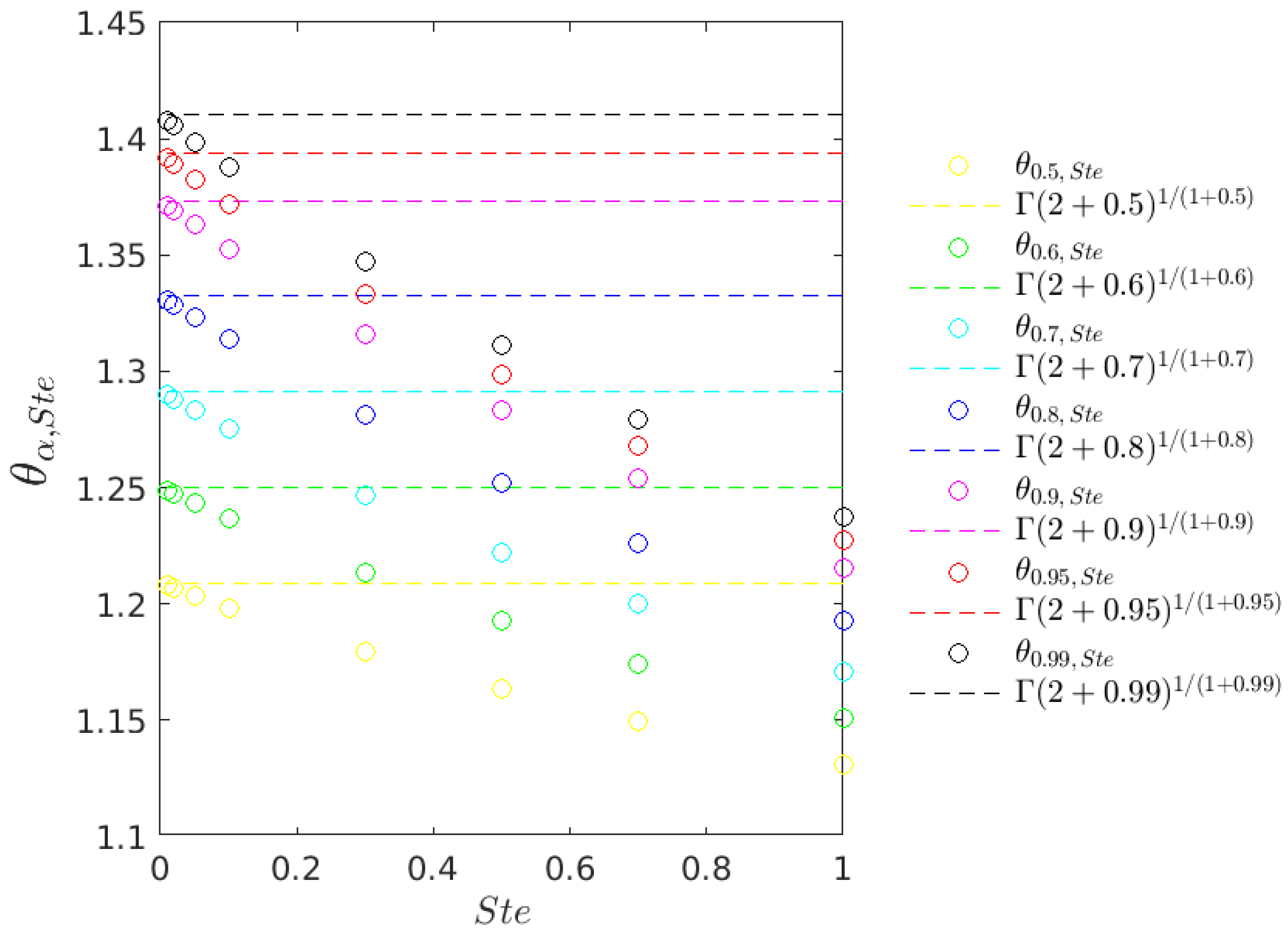
	Ste	1.00	0.70	0.50	0.30	0.10	0.05	0.02	0.01	0
α
0.50		1.1311	1.1493	1.1635	1.1797	1.1984	1.2036	1.2068	1.2079	1.2090
0.60		1.1508	1.1744	1.1926	1.2132	1.2370	1.2435	1.2475	1.2489	1.2503
0.70		1.1711	1.2000	1.2221	1.2470	1.2755	1.2833	1.2882	1.2898	1.2915
0.80		1.1926	1.2264	1.2522	1.2811	1.3141	1.3231	1.3287	1.3306	1.3325
0.90		1.2155	1.2539	1.2830	1.3157	1.3528	1.3629	1.3692	1.3713	1.3734
0.95		1.2276	1.2681	1.2987	1.3331	1.3721	1.3828	1.3894	1.3916	1.3938
0.99		1.2376	1.2796	1.3114	1.3471	1.3876	1.3987	1.4055	1.4078	1.4101

and Figure 1), the next theorem is presented.

Theorem 1. 

The prefactor of the free boundary (45) corresponding to the Space Fractional Stefan Problem (26) converges to the prefactor of the quasi-stationary Space Fractional Stefan problem (38) when the Stefan number approaches zero. In other words,

$$\underset{Ste\to 0}{lim}{\theta }_{\alpha ,Ste}=\mathsf{\Gamma }{(2+\alpha )}^{1/(1+\alpha )}.$$

Proof. 

For every $Ste>0$ let ${\xi }_{\alpha ,Ste}$ be the unique positive solution to (44). Equivalently, ${\xi }_{\alpha ,Ste}$ verifies the equation

$$SteH\left({\xi }_{\alpha ,Ste}\right)={\xi }_{\alpha ,Ste},$$

where H is the function defined in Proposition 2. Let $St{e}_1<St{e}_2$. If we suppose that ${\xi }_{\alpha ,St{e}_2}\le {\xi }_{\alpha ,St{e}_1}$, from Proposition 2 item 3 we deduce that $H\left({\xi }_{\alpha ,St{e}_2}\right)\ge H\left({\xi }_{\alpha ,St{e}_1}\right)$. Then, ${\xi }_{\alpha ,St{e}_2}=St{e}_{2}H\left({\xi }_{\alpha ,St{e}_2}\right)>St{e}_{1}H\left({\xi }_{\alpha ,St{e}_1}\right)={\xi }_{\alpha ,St{e}_1}$, which is a contradiction. Then the family ${\left\{{\xi }_{\alpha ,Ste}\right\}}_{Ste}$ is decreasing respect on the parameter $Ste$ and being the positiveness of the elements we deduce that ${\displaystyle \underset{Ste\to 0}{lim}{\xi }_{\alpha ,Ste}=\beta \ge 0.}$ Now, making $Ste\to 0$ in (44) yields that $0\le \beta {\int }_0^{\beta }{\sigma }_{\alpha }\left(w\right)dw=0,$ and from Proposition 2 we have

$$\underset{Ste\to 0}{lim}{\xi }_{\alpha ,Ste}=0.$$

(47)

Now, using (44) again,

$${\theta }_{\alpha ,Ste}^{1+\alpha }={\left({\displaystyle \frac{{\xi }_{\alpha ,Ste}}{St{e}^{1/(1+\alpha )}}}\right)}^{1+\alpha }={\displaystyle \frac{{\xi }_{\alpha ,Ste}^{\alpha }}{{\int }_0^{{\xi }_{\alpha ,Ste}}{\sigma }_{\alpha }\left(w\right)dw}}·\left({\displaystyle \mathsf{\Gamma }\left(\alpha \right)(1+\alpha )-{\int }_0^{{\xi }_{\alpha ,Ste}}w{\sigma }_{\alpha }\left(w\right)dw}\right).$$

(48)

From (47) and Proposition 2,

$${\displaystyle \underset{Ste\to 0}{lim}\mathsf{\Gamma }\left(\alpha \right)(1+\alpha )-{\int }_0^{{\xi }_{\alpha ,Ste}}w{\sigma }_{\alpha }\left(w\right)dw=\mathsf{\Gamma }\left(\alpha \right)(1+\alpha ).}$$

(49)

By using the series expansion and (47), we compute the limit in the first factor in (48)

$$\underset{Ste\to 0}{lim}{\displaystyle \frac{{\int }_0^{{\xi }_{\alpha ,Ste}}{\sigma }_{\alpha }\left(w\right)dw}{{\xi }_{\alpha ,Ste}^{\alpha }}}=\underset{Ste\to 0}{lim}\left[{\displaystyle \frac{1}{\alpha }}+\sum _{n=1}^{\infty }{\displaystyle \frac{c_n{(-1)}^n}{{(1+\alpha )}^n}}{\displaystyle \frac{{\xi }_{\alpha ,Ste}^{n(1+\alpha )}}{(n+1)(1+\alpha )-1}}\right]={\displaystyle \frac{1}{\alpha }}.$$

(50)

Finally, we make $Ste\to 0$ in (48) and use (49), (50) and the property of the Gamma function saying that $z\mathsf{\Gamma }\left(z\right)=\mathsf{\Gamma }(z+1)$ to obtain

$$\underset{Ste\to 0}{lim}{\theta }_{\alpha ,Ste}=\underset{Ste\to 0}{lim}{\displaystyle \frac{{\xi }_{\alpha ,Ste}}{St{e}^{1/(1+\alpha )}}}={\left(\alpha \mathsf{\Gamma }\left(\alpha \right)(1+\alpha )\right)}^{1/(1+\alpha )}=\mathsf{\Gamma }{(2+\alpha )}^{1/(1+\alpha )}.$$

(51)

□

Corollary 1. 

The solution (42) and (43) to the Space Fractional Stefan Problem (26) converges to the solution (39) to the quasi-stationary Space Fractional Stefan problem (38) when the Stefan number approaches zero.

Proof. 

Going back to (43), we use (51) to claim that

$$\underset{Ste\to 0}{lim}{\tilde{s}}_{\alpha ,Ste}\left(\tau \right)=\underset{Ste\to 0}{lim}{\displaystyle \frac{{\xi }_{\alpha ,Ste}}{St{e}^{\frac{1}{1+\alpha }}}}{\tau }^{{\displaystyle \frac{1}{1+\alpha }}}=\mathsf{\Gamma }{(2+\alpha )}^{{\displaystyle \frac{1}{1+\alpha }}}{\tau }^{{\displaystyle \frac{1}{1+\alpha }}}={\tilde{s}}_{\alpha ,0}\left(\tau \right).$$

For the limit in (42), we use the series expansion approach again

$$\begin{array}{cc}\hfill {\tilde{u}}_{\alpha ,Ste}(y,\tau )& =1-{\displaystyle \frac{{\int }_0^{y/{(\tau /Ste)}^{1/(1+\alpha )}}{\sigma }_{\alpha }\left(w\right)dw}{{\int }_0^{{\xi }_{Ste}}{\sigma }_{\alpha }\left(w\right)dw}}\hfill \\ \hfill & =1-{\displaystyle \frac{{\displaystyle \sum _{n=0}^{\infty }}\frac{c_n{(-1)}^n}{{(1+\alpha )}^n}\frac{y^{(n+1)(1+\alpha )-1}}{(n+1)(1+\alpha )-1}{\left(\frac{Ste}{\tau }\right)}^{\frac{(n+1)(1+\alpha )-1}{1+\alpha }}}{{\displaystyle \sum _{n=0}^{\infty }}\frac{c_n{(-1)}^n}{{(1+\alpha )}^n}\frac{{\xi }_{Ste}^{(n+1)(1+\alpha )-1}}{(n+1)(1+\alpha )-1}}}\hfill \\ \hfill & =1-{\displaystyle \frac{y^{\alpha }}{{\tau }^{\frac{\alpha }{1+\alpha }}}}{\left({\displaystyle \frac{St{e}^{\frac{1}{1+\alpha }}}{{\xi }_{Ste}}}\right)}^{\alpha }{\displaystyle \frac{{\displaystyle \sum _{n=0}^{\infty }}\frac{c_n{(-1)}^n}{{(1+\alpha )}^n}\frac{y^{n(1+\alpha )}}{(n+1)(1+\alpha )-1}{\left(\frac{Ste}{\tau }\right)}^{\frac{n(1+\alpha )}{1+\alpha }}}{{\displaystyle \sum _{n=0}^{\infty }}\frac{c_n{(-1)}^n}{{(1+\alpha )}^n}\frac{{\xi }_{Ste}^{n(1+\alpha )}}{(n+1)(1+\alpha )-1}}}.\hfill \end{array}$$

By applying (47), (51) and the uniform convergence of the series we conclude that

$$\underset{Ste\to 0}{lim}{\tilde{u}}_{\alpha ,Ste}(y,\tau )=1-{\displaystyle \frac{y^{\alpha }}{{\tau }^{\frac{\alpha }{1+\alpha }}}}{\left({\displaystyle \frac{1}{\mathsf{\Gamma }{(2+\alpha )}^{1/(1+\alpha )}}}\right)}^{\alpha }={\tilde{u}}_{\alpha ,0}(y,\tau ).$$

□

5. Computing the Parameter for the Time Fractional Case

5.1. Close Solutions

Let us start by introducing the special functions involved in the representation of the solution for the time fractional case. For more details we refer the reader to [36].

Definition 2. 

For every $y\in [0,1]$, the upper incomplete Beta function of parameters $\alpha ,\beta >0$ is given by

$$\overline{B}(y;\alpha ,\beta )={\int }_y^1{z}^{\alpha -1}{(1-z)}^{\beta -1}dz.$$

Also, the regularized upper incomplete Beta functions is defined by

$$\overline{I}(y;\alpha ,\beta )={\displaystyle \frac{\overline{B}(y;\alpha ,\beta )}{B(\alpha ,\beta )}}.$$

Here, $B(\alpha ,\beta )$ is the classical Beta function defined by $B(\alpha ,\beta )={\int }_0^1{z}^{\alpha -1}{(1-z)}^{\beta -1}dz$.

Remark 7. 

Note that the former functions are not symmetric with respect to the parameters α and β, in contrast to the classical Beta function, which verifies that

$$B(\alpha ,\beta )={\displaystyle \frac{\mathsf{\Gamma }\left(\alpha \right)\mathsf{\Gamma }\left(\beta \right)}{\mathsf{\Gamma }(\alpha +\beta )}}.$$

(52)

Proposition 3. 

For all $0<\alpha <1$, it holds that

$${\int }_0^1\overline{I}\left(z^{2/\alpha };{\displaystyle \frac{\alpha }{2}},1-\alpha \right)dz={\displaystyle \frac{\mathsf{\Gamma }\left(\alpha \right)\mathsf{\Gamma }\left(1-\frac{\alpha }{2}\right)}{\mathsf{\Gamma }\left(\frac{\alpha }{2}\right)}}.$$

Proof. 

Applying Fubini’s theorem, we have that

$$\begin{array}{cc}\hfill {\int }_0^1\overline{I}\left(z^{2/\alpha };{\displaystyle \frac{\alpha }{2}},1-\alpha \right)dz& ={\displaystyle \frac{1}{B\left(\frac{\alpha }{2},1-\alpha \right)}}{\int }_0^1{\int }_{z^{2/\alpha }}^1{w}^{{\displaystyle \frac{\alpha }{2}}-1}{(1-w)}^{-\alpha }dwdz\hfill \\ \hfill & ={\displaystyle \frac{1}{B\left(\frac{\alpha }{2},1-\alpha \right)}}{\int }_0^1{\int }_0^{w^{\alpha /2}}{w}^{{\displaystyle \frac{\alpha }{2}}-1}{(1-w)}^{-\alpha }dzdw,\hfill \end{array}$$

and the thesis holds by using the Beta function definition and (52). □

We start with the quasi-stationary problem. That is, we consider the limit problem obtained from (36) by making $c\to 0$ (or equivalently $Ste\to 0$), which is the time fractional quasi-stationary problem: Find the pair of functions $\tilde{u}:Q_{\tilde{s}}\to \mathbb{R}$ and $\tilde{s}:{\mathbb{R}}_0^{+}\to \mathbb{R}$ with enough regularity such that

$$\begin{array}{ccc}\left(i\right)\hfill & {\displaystyle \frac{1}{\mathsf{\Gamma }(1-\alpha ){(\tau -\tilde{h}\left(y\right))}^{\alpha }}}={\displaystyle \frac{{\partial }^2}{\partial y^2}}\tilde{u}(y,\tau ),\hfill & 0<y<\tilde{s}\left(\tau \right),0<\tau ,\hfill \\ \left(ii\right)\hfill & \tilde{s}\left(0\right)=0,\hfill & \\ \left(iii\right)\hfill & \tilde{u}(0,\tau )=1,\hfill & 0<\tau ,\hfill \\ \left(iv\right)\hfill & \tilde{u}(\tilde{s}\left(\tau \right),\tau )=0,\hfill & 0<\tau ,\hfill \\ \left(v\right)\hfill & {\displaystyle \underset{y\to \tilde{s}{\left(\tau \right)}^{-}}{lim}{\tilde{u}}_y(y,\tau )=0,}\hfill & 0<\tau ,\hfill \end{array}$$

(53)

where $\tilde{h}:{\mathbb{R}}_0\to \mathbb{R}$ is the function given by

$$\tilde{h}\left(y\right)={\tilde{s}}^{-1}\left(y\right),y\ge 0.$$

(54)

Problem (53) was already addressed in [21], where the following solution was obtained:

$$\begin{array}{c}{\displaystyle {\tilde{u}}_{\alpha ,0}(y,\tau )=\frac{2}{\mathsf{\Gamma }(\alpha +1)}\frac{\mathsf{\Gamma }(1+\alpha /2)}{\mathsf{\Gamma }(1-\alpha /2)}{\int }_{\frac{y}{\sqrt{\frac{2}{\mathsf{\Gamma }(\alpha +1)}}{\tau }^{\alpha /2}}}^1\overline{I}(z^{2/\alpha };1-\alpha ,\alpha /2)dz,0\le y\le \tilde{s}\left(\tau \right),0<\tau <T,}\hfill \\ {\tilde{s}}_{\alpha ,0}\left(\tau \right)=\sqrt{{\displaystyle \frac{2}{\mathsf{\Gamma }(1+\alpha )}}}{\tau }^{\alpha /2}.\hfill \end{array}$$

(55)

Regarding the non-stationary problem (36), we must first refer to the work of Kubica and Ryszewska [32], where a similarity solution was obtained. However, unlike the solution here, this solution was not presented in a compact form in terms of calculable transcendental functions. To more clearly see this, we present a self-similar solution following the the lines and steps presented in [32]. To begin, let us recall the formulation of Problem (36).

$$\begin{array}{ccc}\left(i\right)\hfill & Ste{}_{\tilde{h}\left(y\right)}{}^{C\hspace{1em} }D_{\tau }^{\alpha }\tilde{u}(y,\tau )+{\displaystyle \frac{1}{\mathsf{\Gamma }(1-\alpha ){\left(\tau -\tilde{h}\left(y\right)\right)}^{\alpha }}}={\tilde{u}}_{yy}(y,\tau ),\hfill & 0<y<\tilde{s}\left(\tau \right),0<\tau ,\hfill \\ \left(ii\right)\hfill & \tilde{u}(0,\tau )=1,\hfill & 0<\tau ,\hfill \\ \left(iii\right)\hfill & \tilde{u}(\tilde{s}\left(\tau \right),\tau )=0,\hfill & 0<\tau ,\hfill \\ \left(iv\right)\hfill & \tilde{s}\left(0\right)=0,\hfill & \\ \left(v\right)\hfill & {\tilde{u}}_y(\tilde{s}{\left(\tau \right)}^{-},\tau )=0,\hfill & 0<\tau .\hfill \end{array}$$

(56)

Let us define the single-variable function in terms of a self-similar variable (which is different from the one considered in [32]).

$$F\left(\mu \right):=\tilde{u}(y,\tau ),\mu ={\displaystyle \frac{y}{a{\tau }^{\alpha /2}}}.$$

And let the free boundary be given by

$$\tilde{s}\left(\tau \right)=a{\tau }^{\alpha /2}(\mathrm{and}\tilde{h}\left(y\right)={(y/a)}^{2/\alpha }).$$

Remark 8. 

We have made a simplification in the notation by denoting $a:={\theta }_{\alpha ,Ste}$, with the aim to simplify the reading of the next computations. And the correct notation will be recovered at the end of this section.

We have

$$\begin{array}{cc}\hfill {\tilde{u}}_{\tau }(y,\tau )& =F^{\prime }\left(\mu \right)\left(-{\displaystyle \frac{\alpha }{2}}\right){\displaystyle \frac{y}{a{\tau }^{\alpha /2+1}}},\hfill \end{array}$$

(57)

$$\begin{array}{cc}\hfill {\tilde{u}}_y(y,\tau )& =F^{\prime }\left(\mu \right){\displaystyle \frac{1}{a{\tau }^{\alpha /2}}},\hfill \end{array}$$

(58)

$$\begin{array}{cc}\hfill {\tilde{u}}_{yy}(y,\tau )& =F^{″}\left(\mu \right){\displaystyle \frac{1}{a^2{\tau }^{\alpha }}}.\hfill \end{array}$$

(59)

From the boundary condition (56)-$\left(iv\right)$ and making the substitution $\eta =p\tau$, it holds that

$$\begin{array}{cc}\hfill {}_{\tilde{h}\left(y\right)}{}^{C\hspace{1em} }D_{\tau }^{\alpha }\tilde{u}(y,\tau )& ={}_{\tilde{h}\left(y\right)}I_{\tau }^{1-\alpha }{\tilde{u}}_{\tau }(y,\tau )\hfill \\ \hfill & ={\displaystyle \frac{1}{\mathsf{\Gamma }(1-\alpha )}}{\int }_{\tilde{h}\left(y\right)}^{\tau }{F}^{\prime }\left({\displaystyle \frac{y}{a{\eta }^{\alpha /2}}}\right)\left(-{\displaystyle \frac{\alpha }{2}}\right){\displaystyle \frac{y}{a{\eta }^{\alpha /2+1}}}{(\tau -\eta )}^{-\alpha }d\eta \hfill \\ \hfill & =-{\displaystyle \frac{\alpha /2}{\mathsf{\Gamma }(1-\alpha )}}{\int }_{{\left({\displaystyle \frac{y}{a{\tau }^{\alpha /2}}}\right)}^{2/\alpha }}^1{F}^{\prime }\left({\displaystyle \frac{y}{a{\tau }^{\alpha /2}}}{\displaystyle \frac{1}{p^{\alpha /2}}}\right){\displaystyle \frac{y}{a{\left(\tau p\right)}^{\alpha /2+1}}}{t}^{-\alpha }{(1-p)}^{-\alpha }\tau dp\hfill \\ \hfill & =-{\tau }^{-\alpha }{\displaystyle \frac{\alpha /2}{\mathsf{\Gamma }(1-\alpha )}}{\int }_{{\mu }^{2/\alpha }}^1{F}^{\prime }\left(\mu p^{-\alpha /2}\right)\mu p^{-\alpha /2-1}{(1-p)}^{-\alpha }dp.\hfill \end{array}$$

Also,

$$\begin{array}{c}\hfill {\displaystyle \frac{1}{\mathsf{\Gamma }(1-\alpha ){(\tau -\tilde{h}\left(y\right))}^{\alpha }}}={\displaystyle \frac{{\tau }^{-\alpha }}{\mathsf{\Gamma }(1-\alpha )}}{\displaystyle \frac{1}{{(1-{\left(\frac{y}{a{\tau }^{\alpha /2}}\right)}^{2/\alpha })}^{\alpha }}}={\displaystyle \frac{{\tau }^{-\alpha }}{\mathsf{\Gamma }(1-\alpha )}}{\displaystyle \frac{1}{{(1-{\mu }^{2/\alpha })}^{\alpha }}}.\end{array}$$

Then u is a solution to the fractional PDE (56)-$\left(i\right)$ if and only if F is a solution to the fractional ODE

$$\begin{array}{cc}\hfill -a^{-2}{\tau }^{-\alpha }{F}^{″}\left(\mu \right)& ={\displaystyle \frac{Ste·\alpha /2}{\mathsf{\Gamma }(1-\alpha )}}{\tau }^{-\alpha }\mu {\int }_{{\mu }^{2/\alpha }}^1{F}^{\prime }\left(\mu p^{-\alpha /2}\right)p^{-\alpha /2-1}{(1-p)}^{-\alpha }dp\hfill \\ \hfill & -{\displaystyle \frac{{\tau }^{-\alpha }}{\mathsf{\Gamma }(1-\alpha ){(1-{\mu }^{2/\alpha })}^{\alpha }}},\hfill \end{array}$$

or equivalently

$$-F^{″}\left(\mu \right)={\displaystyle \frac{Ste·a^2}{\mathsf{\Gamma }(1-\alpha )}}{\int }_{\mu }^1{F}^{\prime }\left(w\right){\left(1-{\left({\displaystyle \frac{\mu }{w}}\right)}^{2/\alpha }\right)}^{-\alpha }dw-{\displaystyle \frac{a^2}{\mathsf{\Gamma }(1-\alpha ){(1-{\mu }^{2/\alpha })}^{\alpha }}}.$$

(60)

Note that condition (56)-$\left(iv\right)$ implies that $F^{\prime }\left(1\right)=0$. Then, integrating (60) between $\mu$ and 1 yields

$$F^{\prime }\left(\mu \right)={\displaystyle \frac{Ste·a^2}{\mathsf{\Gamma }(1-\alpha )}}{\int }_{\mu }^1{\int }_z^1{F}^{\prime }\left(w\right){\left(1-{\left({\displaystyle \frac{z}{w}}\right)}^{2/\alpha }\right)}^{-\alpha }dwdz-{\displaystyle \frac{a^2}{\mathsf{\Gamma }(1-\alpha )}}{\int }_{\mu }^1{(1-z^{2/\alpha })}^{-\alpha }dz.$$

(61)

Let us work with the integrals in the r.h.s of (61) starting from the second one.

$$\begin{array}{cc}\hfill {\displaystyle \frac{1}{\mathsf{\Gamma }(1-\alpha )}}{\int }_{\mu }^1{(1-z^{2/\alpha })}^{-\alpha }dz& ={\displaystyle \frac{1}{\mathsf{\Gamma }(1-\alpha )}}{\int }_{{\mu }^{2/\alpha }}^1{\displaystyle \frac{\alpha }{2}}{y}^{\alpha /2-1}{(1-y)}^{-\alpha }dy\hfill \\ \hfill & ={\displaystyle \frac{\mathsf{\Gamma }(1+\alpha /2)}{\mathsf{\Gamma }(1-\alpha /2)}}\overline{I}({\mu }^{2/\alpha };\alpha /2,1-\alpha ).\hfill \end{array}$$

(62)

In the first one we apply Fubini and proceed as in (62) to obtain

$$\begin{array}{cc}\hfill & {\displaystyle \frac{1}{\mathsf{\Gamma }(1-\alpha )}}{\int }_{\mu }^1{\int }_z^1{F}^{\prime }\left(w\right){\left(1-{\left({\displaystyle \frac{z}{w}}\right)}^{2/\alpha }\right)}^{-\alpha }dwdz\hfill \\ \hfill & ={\displaystyle \frac{1}{\mathsf{\Gamma }(1-\alpha )}}{\int }_{\mu }^1{F}^{\prime }\left(w\right){\int }_{\mu }^w{\left(1-{\left({\displaystyle \frac{z}{w}}\right)}^{2/\alpha }\right)}^{-\alpha }dzdw\hfill \\ \hfill & ={\displaystyle \frac{1}{\mathsf{\Gamma }(1-\alpha )}}{\int }_{\mu }^1{F}^{\prime }\left(w\right){\int }_{(\mu /w)}^1{\left(1-y^{2/\alpha }\right)}^{-\alpha }wdydw\hfill \end{array}$$

(63)

$$\begin{array}{cc}\hfill & ={\displaystyle \frac{\mathsf{\Gamma }(1+\alpha /2)}{\mathsf{\Gamma }(1-\alpha /2)}}{\int }_{\mu }^1{F}^{\prime }\left(w\right)w\overline{I}\left({\left({\displaystyle \frac{\mu }{w}}\right)}^{2/\alpha };{\displaystyle \frac{\alpha }{2}},1-\alpha \right)dw.\hfill \end{array}$$

(64)

By replacing (62) and (64) in (61) we obtain

$$F^{\prime }\left(\mu \right)={\displaystyle \frac{a^2\mathsf{\Gamma }(1+\alpha /2)}{\mathsf{\Gamma }(1-\alpha /2)}}\left[Ste{\int }_{\mu }^1{F}^{\prime }\left(w\right)w\overline{I}\left({\left({\displaystyle \frac{\mu }{w}}\right)}^{2/\alpha };{\displaystyle \frac{\alpha }{2}},1-\alpha \right)dw-\overline{I}({\mu }^{2/\alpha };\alpha /2,1-\alpha )\right].$$

Now, proceeding as in [32] (Section 5.3), we define the function

$$\begin{array}{c}\hfill G\left(\mu \right)=a^2{\displaystyle \frac{\mathsf{\Gamma }(1+\alpha /2)}{\mathsf{\Gamma }(1-\alpha /2)}}\overline{I}({\mu }^{2/\alpha };\alpha /2,1-\alpha ),\end{array}$$

and the operator $L:C^1[0,1]\to C^1[0,1]$ such that

$$\begin{array}{c}\hfill \left(Lj\right)\left(\mu \right)=Ste{a}^2{\displaystyle \frac{\mathsf{\Gamma }(1+\alpha /2)}{\mathsf{\Gamma }(1-\alpha /2)}}{\int }_{\mu }^{1}j\left(w\right)w\overline{I}\left({\left({\displaystyle \frac{\mu }{w}}\right)}^{2/\alpha };{\displaystyle \frac{\alpha }{2}},1-\alpha \right)dw,\forall j\in C^1[0,1].\end{array}$$

(65)

Then, $F^{\prime }$ verifies

$$F^{\prime }\left(\mu \right)=\left(L{F}^{\prime }\right)\left(\mu \right)-G\left(\mu \right),\forall \mu \in [0,1].$$

(66)

It is important to recall that we have written the operator L and the function G in terms of the incomplete Beta function, but the work and estimates performed in Sections 5.3 and 5.4 of [32] are valid for these expressions. The recursive argument is also valid and consists of applying the operator L to both sides of Equation (66), and we can use Equation (66) to recover a new equation for $F^{\prime }$n-times, yielding

$${\displaystyle F^{\prime }\left(\mu \right)=\left(L^n{F}^{\prime }\right)\left(\mu \right)-\sum _{k=0}^n\left(L^{k}G\right)\left(\mu \right),\forall n\in \mathbb{N}.}$$

(67)

In [32] (Secc.5.2) it was proved that taking the limit when $n\to \infty$ in (67) yields that

$${\displaystyle F^{\prime }\left(\mu \right)=-\sum _{n=0}^{\infty }\left(L^{n}G\right)\left(\mu \right).}$$

(68)

And integrating between $\mu$ and 1 and using condition (36)-$\left(iii\right)$ we obtain an expression for F, which is

$${\displaystyle F\left(\mu \right)={\int }_{\mu }^1\sum _{n=0}^{\infty }\left(L^{n}G\right)\left(z\right)dz.}$$

The uniform convergence of the series in (68) as well as the regularity of function F were analyzed in the mentioned paper. We now look for the parameter a by using the boundary condition (56)-$\left(ii\right)$. In other words, we look for a positive value a such that

$${\displaystyle 1={\int }_0^1\sum _{n=0}^{\infty }\left(L^{n}G\right)\left(z\right)dz,}$$

(69)

where from (65) and denoting $C_{\alpha }:={\displaystyle \frac{\mathsf{\Gamma }(1+\alpha /2)}{\mathsf{\Gamma }(1-\alpha /2)}}$, the operators $L^n$ are given by

$$L^{n}G\left(\mu \right)=Ste{a}^2{C}_{\alpha }{\int }_{\mu }^1\left[L^{n-1}G\right]\left(w\right)w\overline{I}\left({\left({\displaystyle \frac{\mu }{w}}\right)}^{2/\alpha };{\displaystyle \frac{\alpha }{2}},1-\alpha \right)dw,$$

for $n\in \mathbb{N}$ and we define $L^0$ as $L^{0}G\left(\mu \right)=G\left(\mu \right)$.

In order to obtain an expression in terms of the powers of the parameter $Ste·a^2{C}_{\alpha }$, we redefine the operators $L^n$ as follows. First, we define

$${\tilde{L}}^{0}j\left(\mu \right)=\overline{I}({\mu }^{2/\alpha };\alpha /2,1-\alpha ),{\tilde{L}}^{n}j\left(\mu \right)={\int }_{\mu }^1\left[{\tilde{L}}^{(n-1)}j\right]\left(w\right)w\overline{I}\left({\left({\displaystyle \frac{\mu }{w}}\right)}^{2/\alpha };{\displaystyle \frac{\alpha }{2}},1-\alpha \right)dw,$$

(70)

and then we replace it in (69), multiply both sides by $Ste$, and we deduce that the prefactor a verifies that

$${\displaystyle Ste=Ste·a^2{C}_{\alpha }\sum _{n=0}^{\infty }{b}_n{\left(Ste{a}^2{C}_{\alpha }\right)}^n,b_n={\int }_0^1{\tilde{L}}^{n}G\left(z\right)dz.}$$

(71)

Now, define the function

$${\displaystyle \mathcal{H}\left(y\right)=\sum _{n=0}^{\infty }{b}_n{y}^n,0\le y\le 1.}$$

(72)

We know from [32] (Secc- 5.2) that the series in (72) is absolutely convergent and thus the function $\mathcal{H}$ is a well defined continuous function. Moreover, $\mathcal{H}$ is an increasing and positive function. Thus, the equation

$$y\mathcal{H}\left(y\right)=Ste,$$

(73)

admits a unique positive solution, named $y_{Ste}$ and we can recover a asking $y_{Ste}$ that

$$y_{Ste}=Ste·a^2{C}_{\alpha }.$$

More precisely, recalling the definition of $C_{\alpha }$, we state that the prefactor a is given by

$$a=\sqrt{{\displaystyle \frac{\mathsf{\Gamma }(1-\alpha /2)}{\mathsf{\Gamma }(1+\alpha /2)}}{\displaystyle \frac{y_{Ste}}{Ste}}}.$$

(74)

From the previous analysis we can state that the solution to problem (56) is given by the pair

$$\begin{array}{cc}\hfill {\tilde{u}}_{\alpha ,Ste}(y,\tau )& {\displaystyle ={\int }_{y/a{\tau }^{\alpha /2}}^1\sum _{n=0}^{\infty }\left(L^{n}G\right)\left(z\right)dz,}\hfill \end{array}$$

(75)

$$\begin{array}{cc}\hfill {\tilde{s}}_{\alpha ,Ste}\left(\tau \right)& ={\theta }_{\alpha ,Ste}{\tau }^{\alpha /2}.\hfill \end{array}$$

(76)

where ${\theta }_{\alpha ,Ste}:=a$ is defined by (74) and $y_{Ste}$ is the unique solution to Equation (73).

5.2. Computing ${\theta }_{\alpha ,Ste}$

In this section, we outline the elements needed to compute the prefactor a. i.e., the coefficients $b_n$. After this computation, the value of a is achieved using the nonlinear Equation (73) in a similar way to before (see [35] for details on the computation).

For that purpose, let us focus on the coefficients $b_n$ defined in (71).

Proposition 4. 

For every $n\in \mathbb{N}$ the coefficients $b_n$ defined in (71) verify that

$$b_n=\prod _{i=1}^{n+1}\left({\int }_0^1{t}^{2(i-1)}\overline{I}\left(t^{2/\alpha },{\displaystyle \frac{\alpha }{2}},1-\alpha \right)dt\right).$$

(77)

Proof. 

We prove first that, for every $k=0,\dots ,n-1$

$$\begin{array}{cc}\hfill & {\int }_0^1{\tilde{L}}^{n-k}G\left(z\right)z^{2k}dz={\int }_0^1{\tilde{L}}^{n-(k+1)}G\left(z\right)z^{2(k+1)}dz·{\int }_0^1{t}^{2k}\overline{I}\left(t^{2/\alpha },{\displaystyle \frac{\alpha }{2}},1-\alpha \right)dt.\hfill \end{array}$$

In fact, applying (70), Fubini’s Theorem and making the substitution $z=tw$ in the penultimate equality, we obtain

$$\begin{array}{cc}\hfill {\int }_0^1{\tilde{L}}^{n-k}G\left(z\right)z^{2k}dz& ={\int }_0^1\tilde{L}\left({\tilde{L}}^{n-k-1}G\right)\left(z\right)z^{2k}dz\hfill \\ \hfill & ={\int }_0^1{\int }_z^1{\tilde{L}}^{n-k-1}G\left(w\right)w\overline{I}\left({\left({\displaystyle \frac{z}{w}}\right)}^{2/\alpha },{\displaystyle \frac{\alpha }{2}},1-\alpha \right)z^{2k}dwdz\hfill \\ \hfill & ={\int }_0^1{\int }_0^w{\tilde{L}}^{n-k-1}G\left(w\right)w\overline{I}\left({\left({\displaystyle \frac{z}{w}}\right)}^{2/\alpha },{\displaystyle \frac{\alpha }{2}},1-\alpha \right)z^{2k}dzdw\hfill \\ \hfill & ={\int }_0^1{\tilde{L}}^{n-k-1}G\left(w\right)w{\int }_0^w\overline{I}\left({\left({\displaystyle \frac{z}{w}}\right)}^{2/\alpha },{\displaystyle \frac{\alpha }{2}},1-\alpha \right)z^{2k}dzdw\hfill \\ \hfill & ={\int }_0^1{\tilde{L}}^{n-k-1}G\left(w\right)w{\int }_0^1\overline{I}\left(t^{2/\alpha },{\displaystyle \frac{\alpha }{2}},1-\alpha \right)t^{2k}{w}^{2k}wdtdw\hfill \\ \hfill & ={\int }_0^1{\tilde{L}}^{n-(k+1)}G\left(w\right)w^{2(k+1)}dw{\int }_0^1{t}^{2k}\overline{I}\left(t^{2/\alpha },{\displaystyle \frac{\alpha }{2}},1-\alpha \right)dt.\hfill \end{array}$$

Repeating the former argument $n-$times and using (70), we obtain

$$\begin{array}{cc}\hfill b_n& ={\int }_0^1{\tilde{L}}^{n}G\left(z\right)dz\hfill \\ \hfill & ={\int }_0^1{\tilde{L}}^{n-1}G\left(w\right)w^{2}dw{\int }_0^1{t}^{2.0}\overline{I}\left(t^{2/\alpha },{\displaystyle \frac{\alpha }{2}},1-\alpha \right)dt\hfill \\ \hfill & ={\int }_0^1{\tilde{L}}^{n-2}G\left(w\right)w^{2.2}dw{\int }_0^1{t}^{2.1}\overline{I}\left(t^{2/\alpha },{\displaystyle \frac{\alpha }{2}},1-\alpha \right)dt·{\int }_0^1{t}^{2.0}\overline{I}\left(t^{2/\alpha },{\displaystyle \frac{\alpha }{2}},1-\alpha \right)dt\hfill \\ \hfill & =\dots \hfill \\ \hfill & ={\int }_0^1{\tilde{L}}^{0}G\left(w\right)w^{2n}dw\prod _{i=1}^n\left({\int }_0^1{t}^{2(i-1)}\overline{I}\left(t^{2/\alpha },{\displaystyle \frac{\alpha }{2}},1-\alpha \right)dt\right)\hfill \\ \hfill & ={\int }_0^1\overline{I}\left(w^{2/\alpha },{\displaystyle \frac{\alpha }{2}},1-\alpha \right)w^{2n}dw·\prod _{i=1}^n\left({\int }_0^1{t}^{2(i-1)}\overline{I}\left(t^{2/\alpha },{\displaystyle \frac{\alpha }{2}},1-\alpha \right)dt\right)\hfill \\ \hfill & =\prod _{i=1}^{n+1}\left({\int }_0^1{t}^{2(i-1)}\overline{I}\left(t^{2/\alpha },{\displaystyle \frac{\alpha }{2}},1-\alpha \right)dt\right),\hfill \end{array}$$

which completes the proof. □

We also present the following property needed for the next section.

Proposition 5. 

For all $n\in {\mathbb{N}}_0$, it holds that $b_n>0$.

Proof. 

It immediately follows from the positiveness of

$${\tilde{L}}^{0}G\left(z\right)=\overline{I}\left(z^{2/\alpha };{\displaystyle \frac{\alpha }{2}},1-\alpha \right)>0,\forall z\ne 1,$$

and formula (77). □

5.3. Analysis of the Convergence to the Quasi-Stationary Case

Following a similar approach presented in Section 4.3, looking at the results in Figure 2 and

Table 3. Time Fractional Stefan Problem. Different values of ${\theta }_{\alpha ,Ste}:=\sqrt{{\displaystyle \frac{\mathsf{\Gamma }(1-\alpha /2)y_{Ste}}{\mathsf{\Gamma }(1+\alpha /2)Ste}}}$ (central box) and $\sqrt{{\displaystyle \frac{2}{\mathsf{\Gamma }(1+\alpha )}}}$ (right column).

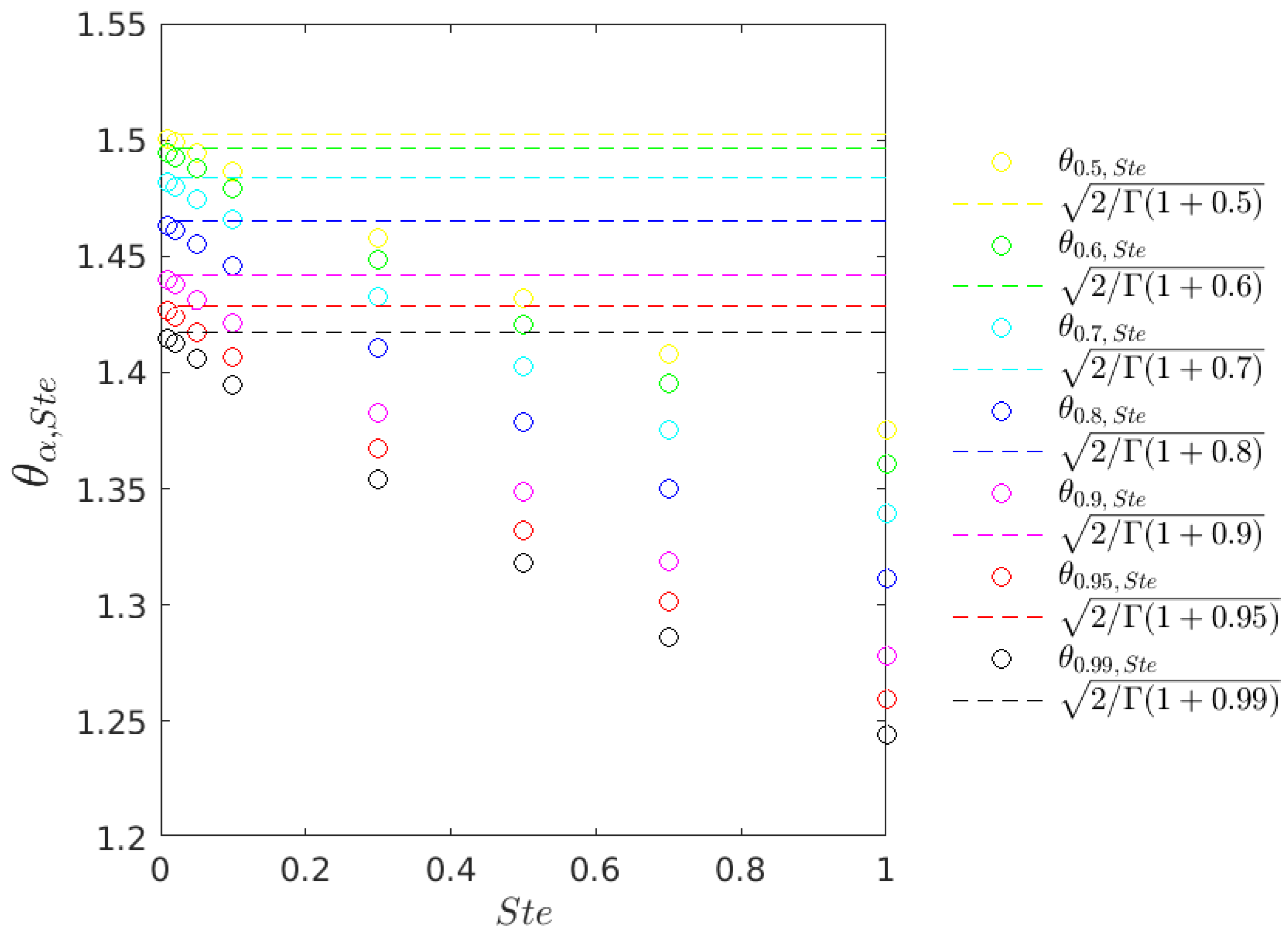
	Ste	1.00	0.70	0.50	0.30	0.10	0.05	0.02	0.01	0
α
0.50		1.3751	1.4077	1.4318	1.4580	1.4867	1.4944	1.4991	1.5007	1.5023
0.60		1.3606	1.3951	1.4206	1.4485	1.4794	1.4876	1.4927	1.4944	1.4961
0.70		1.3391	1.3755	1.4026	1.4324	1.4656	1.4744	1.4799	1.4818	1.4836
0.80		1.3114	1.3498	1.3786	1.4103	1.4459	1.4555	1.4614	1.4634	1.4654
0.90		1.2782	1.3186	1.3490	1.3829	1.4210	1.4313	1.4377	1.4399	1.4421
0.95		1.2598	1.3011	1.3324	1.3673	1.4068	1.4175	1.4242	1.4264	1.4287
0.99		1.2441	1.2863	1.3183	1.3540	1.3946	1.4057	1.4125	1.4149	1.4172

, and recalling (37), the analysis of convergence will be stated by making $Ste\to 0$.

Theorem 2. 

The prefactor of the free boundary in Equation (76) associated with the Time Fractional Stefan Problem (56) converges to the prefactor of the quasi-stationary Time Fractional Stefan Problem (53) as the Stefan number tends to zero. That is,

$$\underset{Ste\to 0}{lim}{\theta }_{\alpha ,Ste}=\sqrt{{\displaystyle \frac{2}{\mathsf{\Gamma }(1+\alpha )}}}.$$

Proof. 

Let $y_{Ste}$ the unique positive solution to $y\mathcal{H}\left(y\right)=Ste$.

By Proposition 5, we deduce that $y_{Ste}\mathcal{H}\left(y_{Ste}\right)>0$, and $\mathcal{H}\left(y_{Ste}\right)\ge b_0>0$. Then, from this comment and equality

$$\underset{Ste\to 0}{lim}{y}_{Ste}\mathcal{H}\left(y_{Ste}\right)=\underset{Ste\to 0}{lim}Ste=0,$$

it holds that $\underset{Ste\to 0}{lim}{y}_{Ste}=0$.

We can now compute the following limit

$$\begin{array}{cc}\hfill \underset{Ste\to 0}{lim}{\displaystyle \frac{y_{Ste}}{Ste}}& =\underset{Ste\to 0}{lim}{\displaystyle \frac{y_{Ste}}{y_{Ste}\mathcal{H}\left(y_{Ste}\right)}}=\underset{Ste\to 0}{lim}{\displaystyle \frac{1}{{\displaystyle \sum _{n=0}^{\infty }{b}_n{y}_{Ste}^n}}}={\displaystyle \frac{1}{b_0}}\hfill \\ \hfill & ={\displaystyle \frac{1}{{\int }_0^1\overline{I}\left(z^{2/\alpha };\frac{\alpha }{2},1-\alpha \right)dz}}={\displaystyle \frac{\mathsf{\Gamma }\left(\frac{\alpha }{2}\right)}{\mathsf{\Gamma }\left(\alpha \right)\mathsf{\Gamma }\left(1-\frac{\alpha }{2}\right)}}.\hfill \end{array}$$

(78)

Returning to (74), and using (78) and the Gamma function property $\mathsf{\Gamma }(z+1)=z\mathsf{\Gamma }\left(z\right)$ several times we obtain

$$\underset{Ste\to 0}{lim}{\theta }_{\alpha ,Ste}=\underset{Ste\to 0}{lim}\sqrt{{\displaystyle \frac{\mathsf{\Gamma }\left(1-\frac{\alpha }{2}\right)}{\mathsf{\Gamma }\left(1+\frac{\alpha }{2}\right)}}{\displaystyle \frac{y_{Ste}}{Ste}}}=\sqrt{{\displaystyle \frac{2}{\mathsf{\Gamma }(1+\alpha )}}}.$$

□

Corollary 2. 

The solution (75) and (76) to the Time Fractional Stefan Problem (56) converges to the solution (55) to the quasi-stationary Time Fractional Stefan problem (53) when the Stefan number approaches zero.

Proof. 

First, note that, being $\overline{I}\left(z;{\displaystyle \frac{\alpha }{2}},1-\alpha \right)\le 1$ for all $0\le z\le 1$, it follows that

$$0\le L^{0}G\left(z\right)={\theta }_{\alpha ,Ste}^2{C}_{\alpha }\overline{I}\left(z^{2/\alpha };{\displaystyle \frac{\alpha }{2}},1-\alpha \right)\le {\theta }_{\alpha ,Ste}^2{C}_{\alpha }.$$

By induction, we deduce that

$$0\le L^{n}G\left(z\right)\le St{e}^n{\theta }_{\alpha ,Ste}^{2(n+1)}{C}_{\alpha }^{n+1}.$$

Then,

$$0\le {\tilde{u}}_{Ste}(y,\tau )={\int }_{{\displaystyle \frac{y}{{\theta }_{\alpha ,Ste}{\tau }^{\alpha /2}}}}^1\sum _{n=0}^{\infty }\left(L^{n}G\right)\left(z\right)dz\le {\int }_{{\displaystyle \frac{y}{{\theta }_{\alpha ,Ste}{\tau }^{\alpha /2}}}}^1\sum _{n=0}^{\infty }St{e}^n{\theta }_{\alpha ,Ste}^{2(n+1)}{C}_{\alpha }^{n+1}dz,$$

and for $Ste<1$ the series in the right-hand-side converges absolutely. Hence, using that $L^{n}G\left(z\right)\to 0$ for all $n\in \mathbb{N}$ when $Ste\to 0$, we obtain that

$$\begin{array}{cc}\hfill \underset{Ste\to 0}{lim}{\tilde{u}}_{Ste}(y,\tau )& =\underset{Ste\to 0}{lim}{\int }_{{\displaystyle \frac{y}{a{\tau }^{\alpha /2}}}}^1\sum _{n=0}^{\infty }\left(L^{n}G\right)\left(z\right)dz\hfill \\ \hfill & ={\displaystyle \frac{\mathsf{\Gamma }\left(1+\frac{\alpha }{2}\right)}{\mathsf{\Gamma }\left(1-\frac{\alpha }{2}\right)}}{\displaystyle \frac{2}{\mathsf{\Gamma }\left(1+\alpha \right)}}{\int }_{{\displaystyle \frac{y}{\sqrt{\frac{2}{\mathsf{\Gamma }\left(1+\alpha \right)}}{\tau }^{\alpha /2}}}}^1\overline{I}\left(z^{2/\alpha };{\displaystyle \frac{\alpha }{2}},1-\alpha \right)dz,\hfill \end{array}$$

and the convergence ${\tilde{u}}_{\alpha ,Ste}\to {\tilde{u}}_{\alpha ,0}$ is proven.

Going back to definition (74) and applying (78) and properties of Gamma function, we obtain that

$$\underset{Ste\to 0}{lim}{\theta }_{\alpha ,Ste}{\tau }^{\alpha /2}=\underset{Ste\to 0}{lim}\sqrt{{\displaystyle \frac{\mathsf{\Gamma }\left(1-\frac{\alpha }{2}\right)}{\mathsf{\Gamma }\left(1+\frac{\alpha }{2}\right)}}{\displaystyle \frac{y_{Ste}}{Ste}}}{\tau }^{\alpha /2}=\sqrt{{\displaystyle \frac{2}{\mathsf{\Gamma }(1+\alpha )}}}{\tau }^{\alpha /2}.$$

□

6. Physical Interpretations

In closing out the analysis, it is worthwhile to provide a physical interpretation of our expressions for the advance of the melt front.

6.1. Integer Case

As a base line we start by considering the integer case, which was presented in (2). In this case, through the classic square root in time diffusional scaling, the dimensionless position of the phase front (dimensions [L]) will advance as

$$s=\theta \lambda t^{{\displaystyle \frac{1}{2}}}$$

So, the movement of the melt front is controlled by the product of a dimensionless prefactor $\theta$ and the square root of the thermal diffusivity. Further, recall that the value of $\theta$ is the positive solution of the transcendental Equation (3) that we rewrite for the benefit of the reader

$${\displaystyle \frac{x}{2}}erf\left({\displaystyle \frac{x}{2}}\right)e^{x^2/4}={\displaystyle \frac{Ste}{\sqrt{\pi }}}.$$

Thus, this parameter is solely a function of the Stefan number (Ste)—the governing dimensionless group for melting phase change problems.

6.2. Space Fractional Derivative

In the case of the space fractional derivative, and on introducing an “extended” definition of the heat diffusivity

$${\lambda }_L^2={\nu }_{\alpha }{\lambda }^2,$$

accounting for the length dimension change induced by the convolution in space of the heat flux, the melt front moves as

$$s\left(t\right)={\theta }_{\alpha ,Ste}{\lambda }_L^{{\displaystyle \frac{2}{1+\alpha }}}{t}^{{\displaystyle \frac{1}{1+\alpha }}},$$

where the values of ${\theta }_{\alpha ,Ste}$ are given in Table 2. This expression has the same form as the integer front movement, involving the product of the following: (i) a dimensionless parameter solely dependent on the value of Ste; (ii) a power of the extended diffusivity, representing the nature of the heat transfer in the system; (iii) a time exponent arising directly from the scaling of the governing Equation (26)-(i) [14].

6.3. Time Fractional Derivative

In the time fractional case, on accounting for the convolution of the flux in time by introducing the “extended” definition of the heat diffusivity

$${\lambda }_T^2={\mu }_{\alpha }{\lambda }^2,$$

the movement of the melt front is given by

$$s\left(t\right)={\theta }_{\alpha ,Ste}{\lambda }_T{t}^{{\displaystyle \frac{\alpha }{2}}},$$

where the values of ${\theta }_{\alpha ,Ste}$ are given in Table 3. Again, consistent with the physical interpretation in the integer and space derivative cases, the first term is a dimensionless prefactor that only depends on the value of the Stefan number, the second term accounts for the contribution of the heat transfer, and the last term accounts for the dependency on time.

7. Conclusions

We have presented self-similar solutions for one-dimensional time and space fractional Stefan melting problems derived from thermal continuity equations. It is well known that when a constant temperature boundary ($x=0$) is applied, and the initial position of the sharp interface is the origin ($s\left(0\right)=0$), these solutions exhibit sub- and super-diffusion behaviors, respectively, i.e., the melt front advance is determined as the product of a prefactor and time to a power n, which is different from the diffusion value of ${\displaystyle \frac{1}{2}}$. In both the fractional time and space cases, the time exponent is given in terms of the known functions of the orders of the space and time derivatives in the problem formulations. The main contribution of the current work has been to, for the first time, make explicit computations for the values of the prefactors. We expect that our analysis will be useful when fractional models for anomalous diffusion are proposed. Additionally, the exact solutions (prefactor values) computed here will be a strong tool for testing numerical methods for fractional free boundary problems.

References

- Tarzia, D.A. A bibliography on moving–free boundary problems for the heat diffusion equation. The Stefan and related problems. MAT—Ser. A 2000, 2, 1–297. [Google Scholar] [CrossRef]
- Alexiades, V.; Solomon, A.D. Mathematical Modelling of Melting and Freezing Processes; Hemisphere: Taylor and Francis: Washington, DC, USA, 1993. [Google Scholar]
- Meirmanov, A. The Stefan Problem; Walter de Gruyter: Berlin, Germany, 1992. [Google Scholar]
- Solomon, A.D. An easily computable solution to a two-phase Stefan problem. J. Sol. Energy 1979, 23, 525–528. [Google Scholar] [CrossRef]
- Zhmakin, A.I. Non-Fourier Heat Conduction. From Phase-Lag Models to Relativistic and Quantum Transport; Springer: Cham, Switzerland, 2023. [Google Scholar]
- Benenti, G.; Donadio, D.; Lepri, S.; Livi, R. Non-Fourier heat transport in nanosystems. Riv. Nuovo Cimento 2023, 46, 105–161. [Google Scholar] [CrossRef]
- Brociek, R.; Słota, D.; Król, M.; Matula, G.; Kwaśny, W. Modeling of Heat Distribution in Porous Aluminum Using Fractional Differential Equation. Fractal Fract. 2017, 1, 17. [Google Scholar] [CrossRef]
- Failla, G.; Zingales, M. Advanced materials modelling via fractional calculus: Challenges and perspectives. Philos. Trans. A Math. Phys. Eng. Sci. 2020, 378, 20200050. [Google Scholar] [CrossRef]
- Feng, Y.; Goree, J.; Liu, B. Identifying anomalous diffusion and melting in dusty plasmas. Phys. Rev. E 2010, 82, 036403. [Google Scholar] [CrossRef]
- Schwarzwälder, M.C.; Myers, T.G.; Hennessy, M.G. The one-dimensional Stefan problem with non-Fourier heat conduction. Int. J. Therm. Sci. 2020, 150, 106210. [Google Scholar] [CrossRef]
- Arya, R.K.; Thapliyal, D.; Sharma, J.; Verros, G.D. Glassy Polymers—Diffusion, Sorption, Ageing and Applications. Coatings 2011, 11, 1049. [Google Scholar] [CrossRef]
- Kukhtetskiy, S.V.; Fomenko, E.V.; Anshits, A.G. Anomalous Diffusion of Helium and Neon in Low-Density Silica Glass. Membranes 2023, 13, 754. [Google Scholar] [CrossRef]
- Eliazar, I.; Klafter, J. Anomalous is ubiquitous. Ann. Phys. 2011, 326, 2517–2531. [Google Scholar] [CrossRef]
- Metzler, R.; Klafter, J. The random walk’s guide to anomalous diffusion: A fractional dynamics approach. Phys. Rev. 2000, 339, 1–77. [Google Scholar] [CrossRef]
- Voller, V.R. Anomalous heat transfer: Examples, fundamentals, and fractional calculus models. In Advances in Heat Transfer; Elsevier: Amsterdam, The Netherlands, 2018; Volume 50, pp. 333–380. [Google Scholar]
- Hilfer, R. Applications of Fractional Calculus in Physics; World Scientific Publishing Company: London, UK, 2000. [Google Scholar]
- Jin, B. Fractional Differential Equations; Springer: Cham, Switzerland, 2021. [Google Scholar]
- Kumar, D.; Singh, J. Fractional Calculus in Medical and Health Science, 1st ed.; CRC Press: Boca Raton, FL, USA, 2020. [Google Scholar]
- Podlubny, I. Fractional Differential Equations; Vol. 198 of Mathematics in Science and Engineering; Academic Press: San Diego, CA, USA, 1999. [Google Scholar]
- Samko, S.; Kilbas, A.; Marichev, O. Fractional Integrals and Derivatives—Theory and Applications; Gordon and Breach: New York, NY, USA, 1993. [Google Scholar]
- Roscani, S.; Voller, V. On an enthalpy formulation for a sharp-interface memory-flux Stefan problem. Chaos Solitons Fractals 2024, 181, 114679. [Google Scholar] [CrossRef]
- Voller, V.R. Fractional Stefan problems. Int. J. Heat Mass Tran. 2014, 74, 269–277. [Google Scholar] [CrossRef]
- Błasik, M.; Klimek, M. Numerical solution of the one phase 1D fractional Stefan problem using the front fixing method. Math. Method Appl. Sci. 2015, 38, 3214–3228. [Google Scholar] [CrossRef]
- Garshasbi, M.; Sanaei, F. Studying a time-fractional moving boundary diffusion model of solvent through a glassy polymer: A computational approach. Int. J. Numer. Model. 2024, 37, e3181. [Google Scholar] [CrossRef]
- Gruber, C.A.; Vogl, C.J.; Miksis, M.J.; Davis, S.H. Anomalous diffusion models in the presence of a moving interface. Interfaces Free Bound 2023, 15, 181–202. [Google Scholar] [CrossRef]
- Kang, J.; Zhou, F.; Xia, T.; Ye, G. Numerical modeling and experimental validation of anomalous time and space subdiffusion for gas transport in porous coal matrix. Int. J. Heat Mass Tran. 2016, 100, 747–757. [Google Scholar] [CrossRef]
- Liu, J.; Xu, M. Some exact solutions to Stefan problems with fractional differential equations. J. Math. Anal. Appl. 2009, 351, 536–542. [Google Scholar] [CrossRef]
- Roscani, S.; Tarzia, D.; Venturato, L. The similarity method and explicit solutions for the fractional space one-phase Stefan problems. Fract. Calc. Appl. Anal. 2022, 25, 995–1021. [Google Scholar] [CrossRef]
- Bertsch, M.; Klaver, M. The Stefan problem with mushy regions: Differentiability of the interfaces. Ann. Mat. Pura Appl. 1994, 166, 27–61. [Google Scholar] [CrossRef]
- Ughi, M. A Melting Problem with a Mushy Region: Qualitative Properties. IMA J. Appl. Math. 1984, 33, 135–152. [Google Scholar] [CrossRef]
- Voller, V.R.; Cross, M.; Markatos, N.C. An enthalpy method for convection/diffusion phase change. Int. J. Numer. Methods Eng. 1987, 24, 271–284. [Google Scholar] [CrossRef]
- Kubica, A.; Ryszewska, K. A self-similar solution to time-fractional Stefan problem. Math. Methods Appl. Sci. 2021, 44, 4245–4275. [Google Scholar] [CrossRef]
- Roscani, S.; Caruso, N.; Tarzia, D. Explicit solutions to fractional Stefan-like problems for Caputo and Riemann–Liouville derivatives. Commun. Nonlinear. Sci. Numer. Simul. 2020, 90, 105361. [Google Scholar] [CrossRef]
- Kilbas, A.A.; Saigo, M. On Mittag-Leffler type function, fractional calculus operators and solutions of integral equations. Integral Transform. Spec. Funct. 1996, 4, 355–370. [Google Scholar] [CrossRef]
- Caruso, N.; Roscani, S.; Venturato, L. carusonahuel/FractionalStefanProblems_Computing_prefactors: Computing prefactors (v1.0.0). Zenodo 2025. [Google Scholar] [CrossRef]
- Srivastava, H.M.; Choi, J. Zeta and q-Zeta Functions and Associated Series and Integrals; Elsevier: London, UK, 2012. [Google Scholar]