

Proposal for the Application of Fractional Operators in Polynomial Regression Models to Enhance the Determination Coefficient R2 on Unseen Data


Abstract
1. Introduction
2. Sets of Fractional Operators
3. Groups of Fractional Operators
4. Polynomial Regression Model
- represents the vector of observed responses;
- is the design matrix, with each row corresponding to an observation and each column representing a specific power of x;
- denotes the vector of regression coefficients.
- The intercept indicates the predicted value of y at .
- The coefficient pertains to the linear term x, governing the slope of the regression line near .
- The coefficient relates to the quadratic term , influencing the curvature of the fit.
- Higher-order coefficients, such as for , for , etc., introduce additional degrees of flexibility, enabling the model to capture more intricate patterns.
5. Seen and Unseen Data in Regression Models
- Overfitting: This occurs when a model excessively adapts to the specific details and noise within the training data, thereby impairing its ability to perform accurately on unseen data. Overfitting is usually linked to models that are overly complex relative to the size or variability of the training set. Consequently, the model becomes too specialized in the training data, losing generalization capacity on new samples.
- Underfitting: This situation arises when the model is overly simplistic and fails to capture the genuine patterns in the data, resulting in poor predictive performance on both the training and test datasets. Underfitting generally happens when the model’s parameterization is insufficient or too rigid to reflect the underlying relationships, causing inaccurate predictions and low overall efficacy.
6. The Coefficient of Determination
- : This indicates a perfect fit where the model explains all variance in the dependent variable. The predicted values coincide exactly with the actual values, implying zero prediction error. However, such a result is uncommon in practical contexts and often suggests overfitting.
- : Values within this interval imply that the model accounts for a portion of the variance. The closer is to 1, the better the fit and the more variance explained. For instance, indicates that 80% of the variance is captured by the model.
- : This value suggests that the model does not explain any variance beyond the mean of the dependent variable. Predictions are no better than simply using the average outcome, indicating no meaningful relationship is captured.
- Negative : Though rare, negative values may occur when the model performs worse than a naive mean predictor. This signals poor model fit and often results from overfitting or incorrect model formulation.
- Enhanced generalization: Models with elevated on unseen data provide reliable predictions for novel observations, increasing practical utility.
- Mitigated overfitting: Sustained high on test sets suggests the model has learned substantive patterns rather than memorizing training instances.
- Improved decision support: In domains such as finance, healthcare, and engineering, dependable predictions based on high test facilitate better informed decisions.
- Robust model selection: Comparing values across models aids in identifying the optimal balance between complexity and predictive accuracy without overfitting.
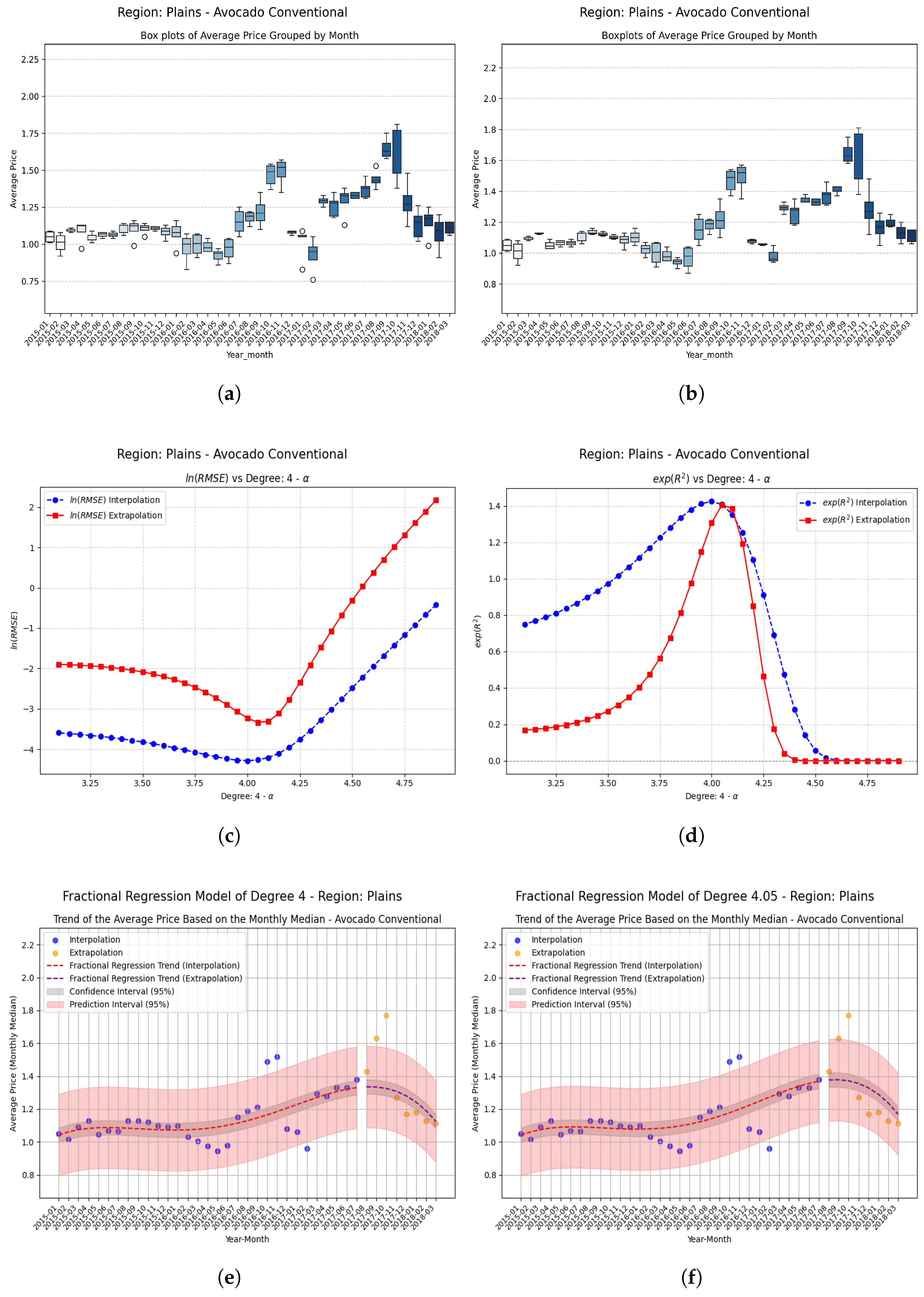
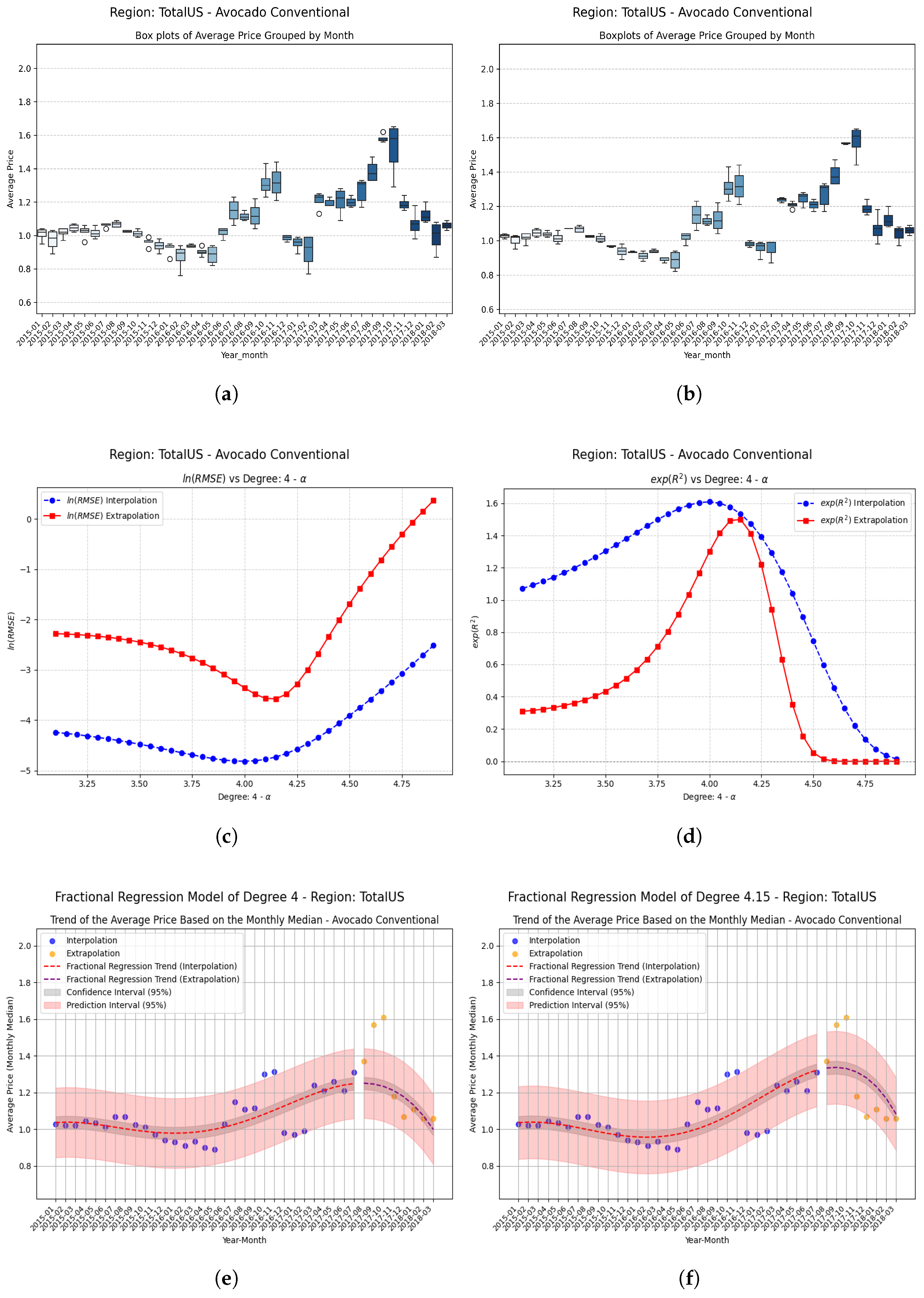
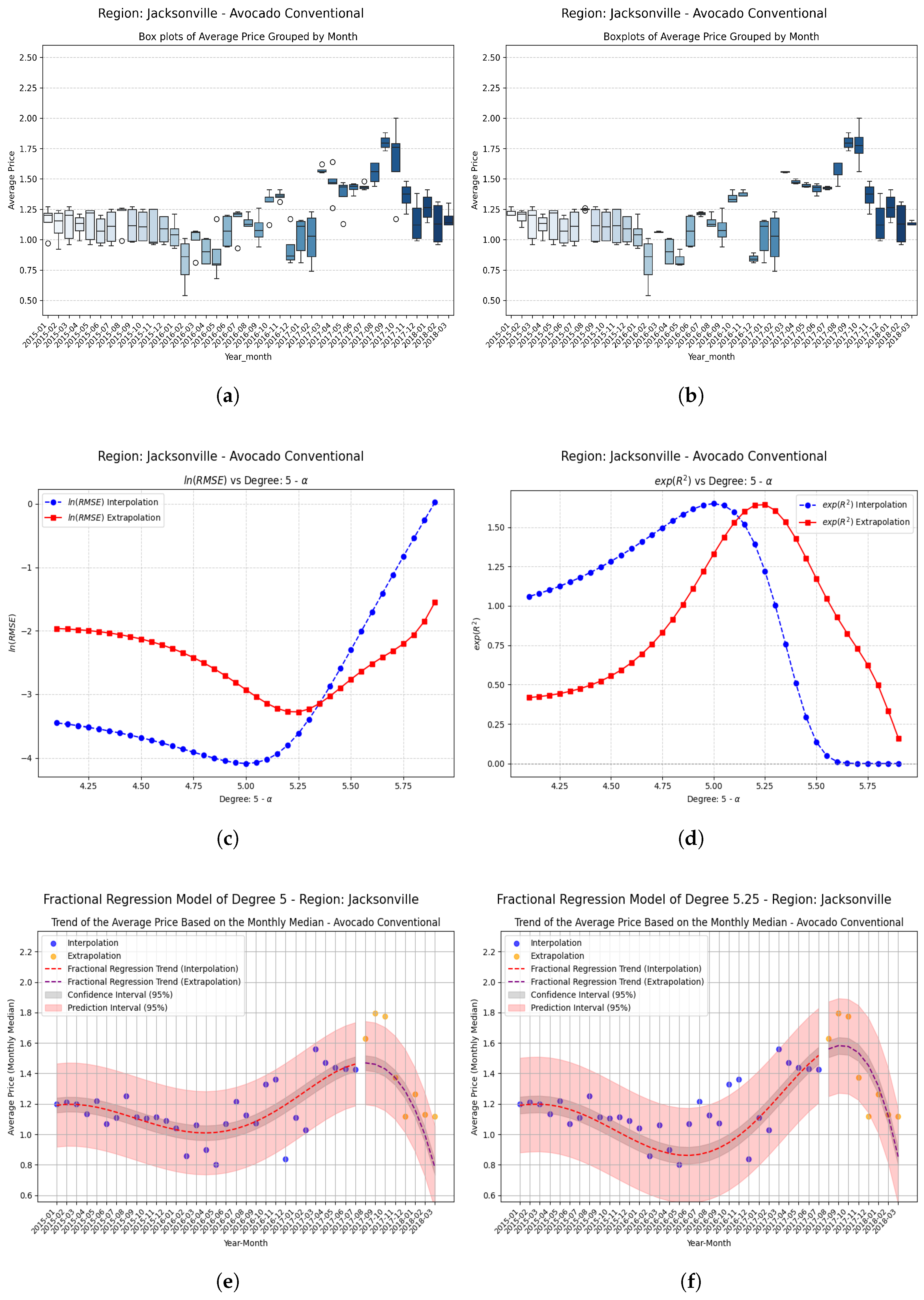
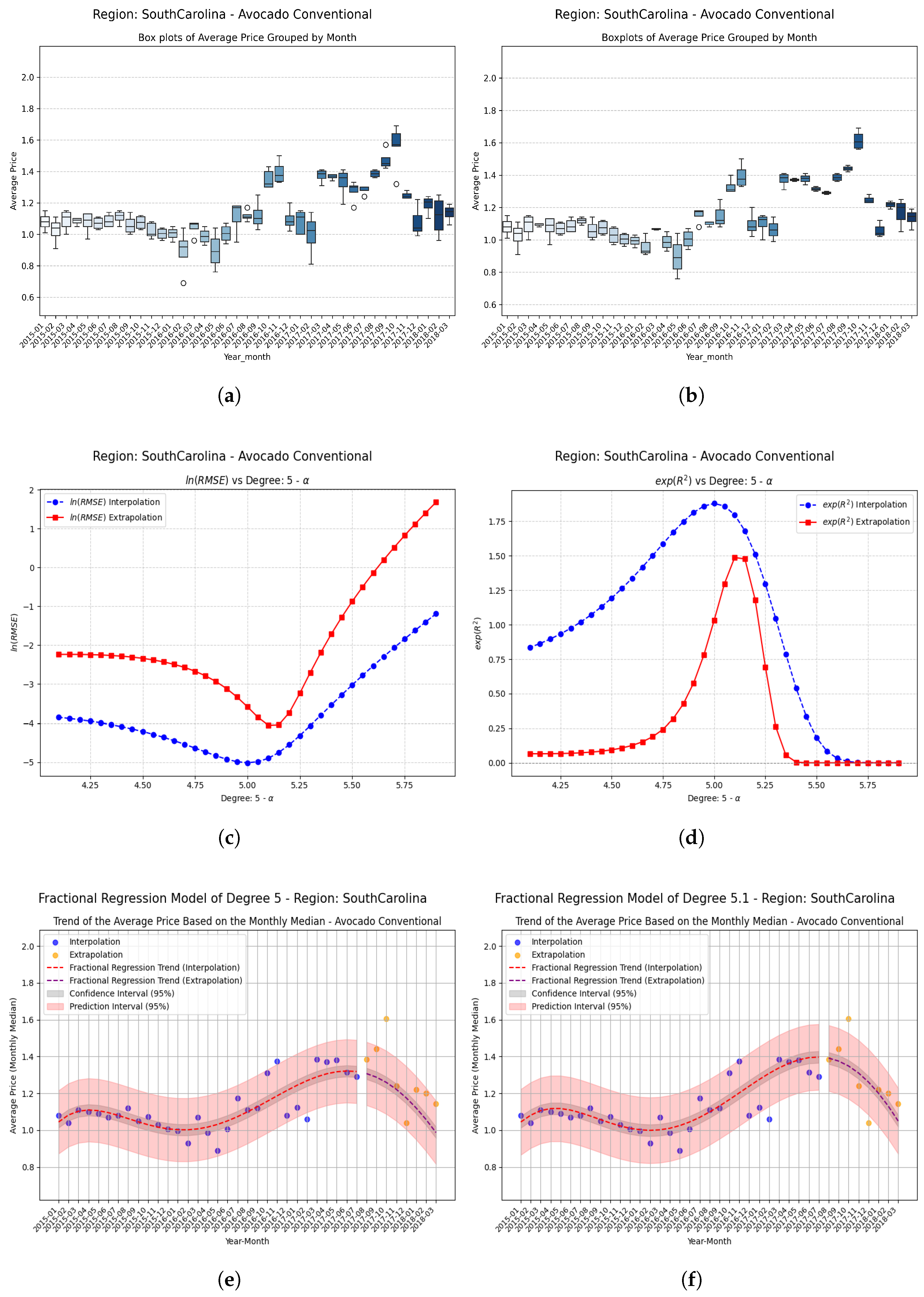
7. Fractional Regression Model
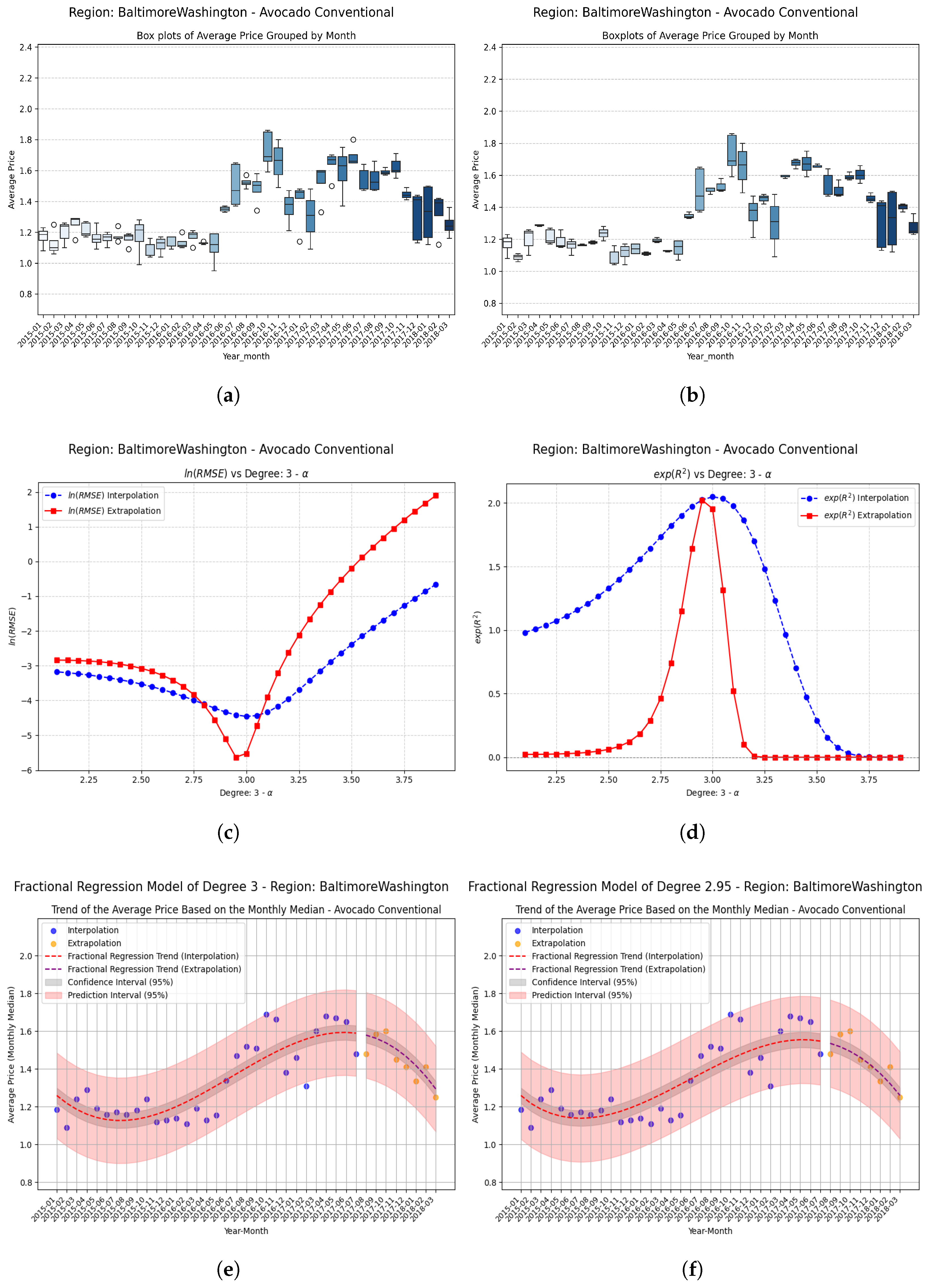
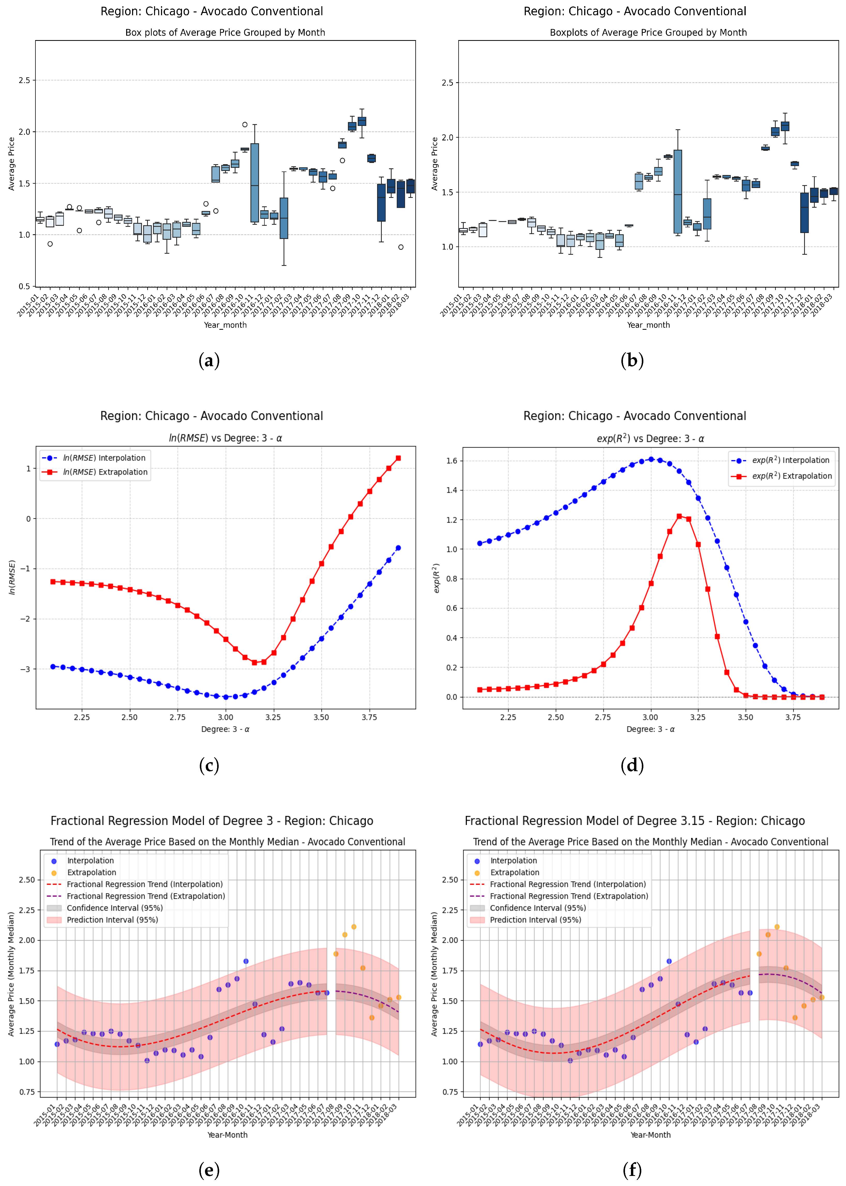
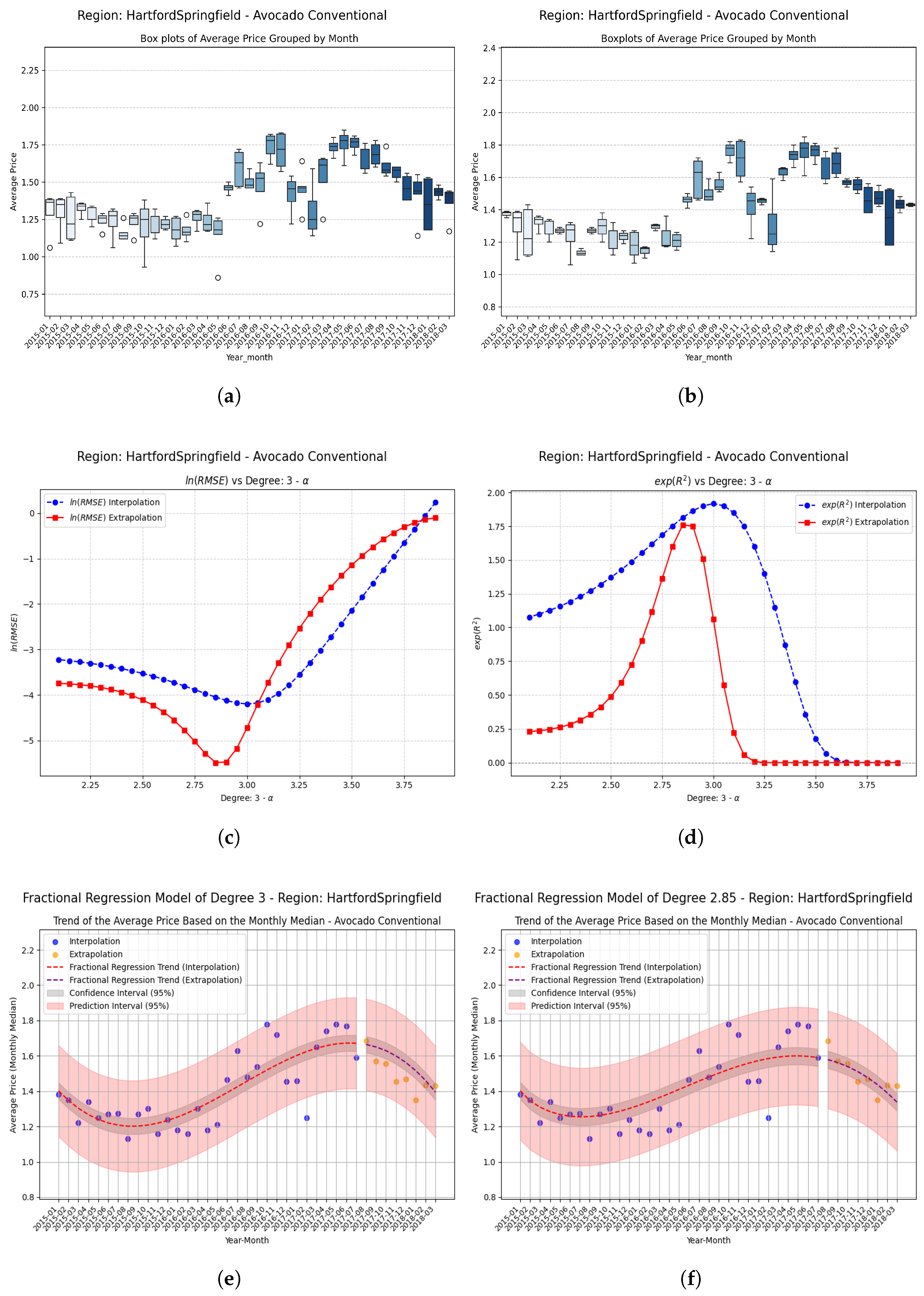
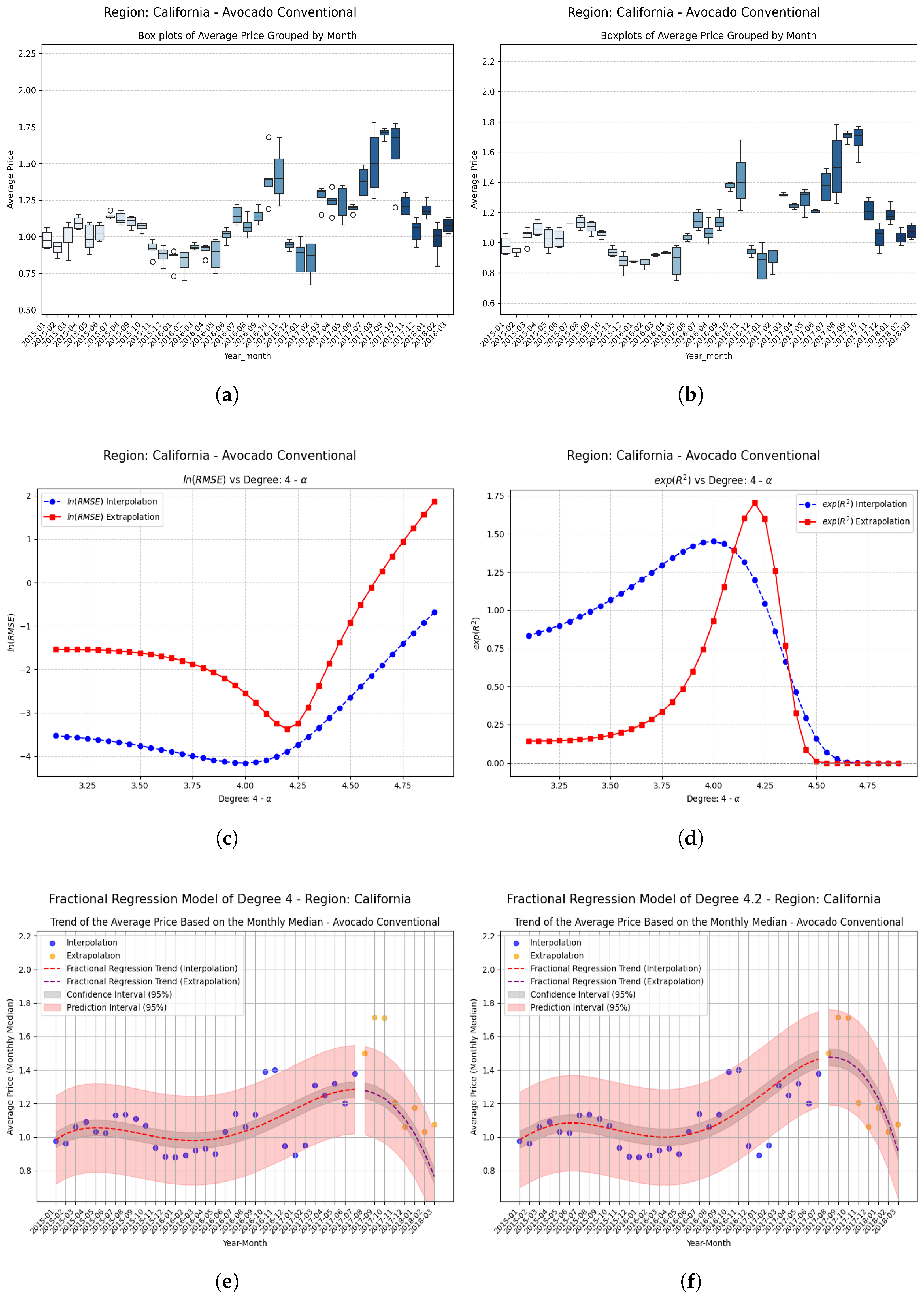
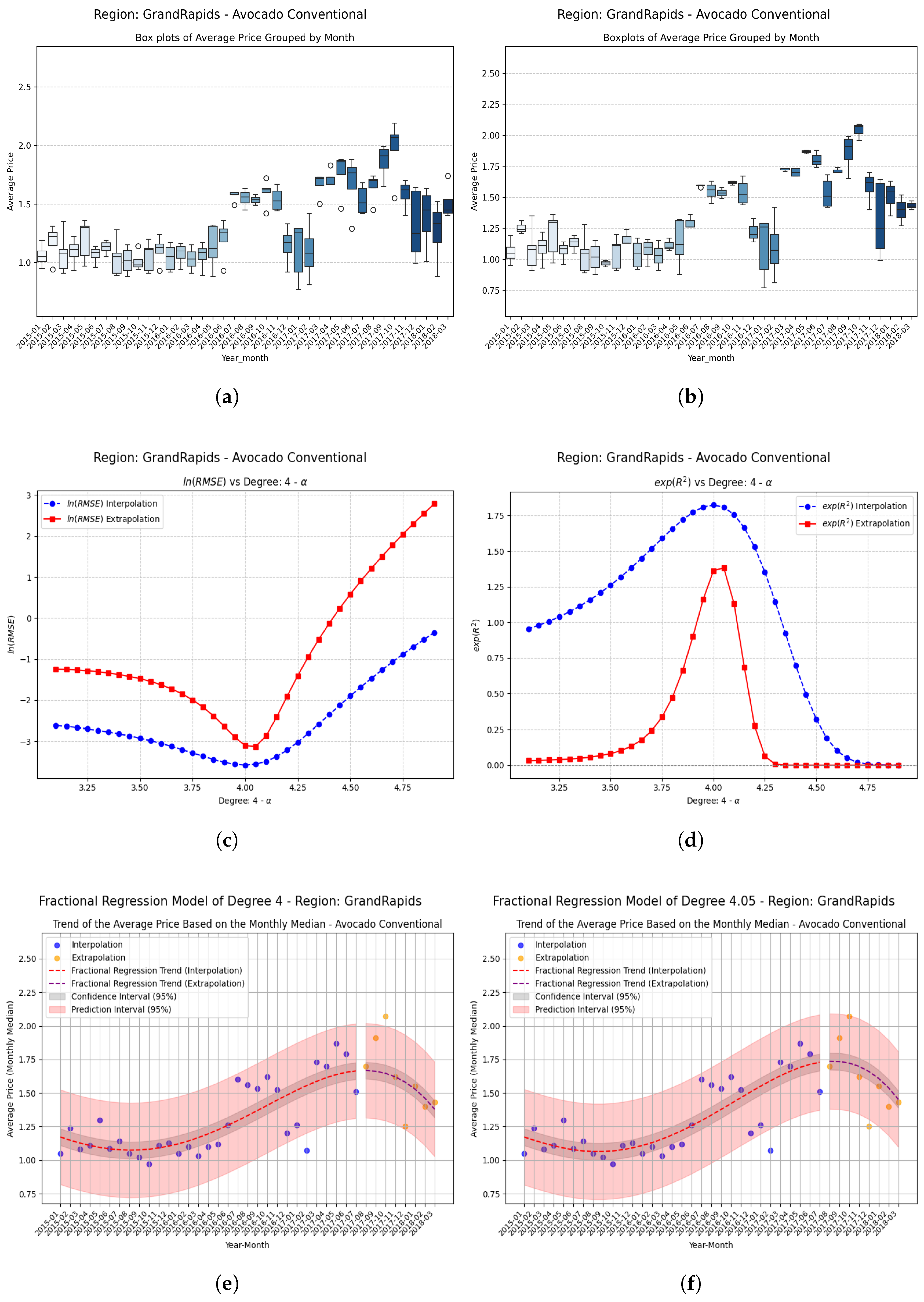
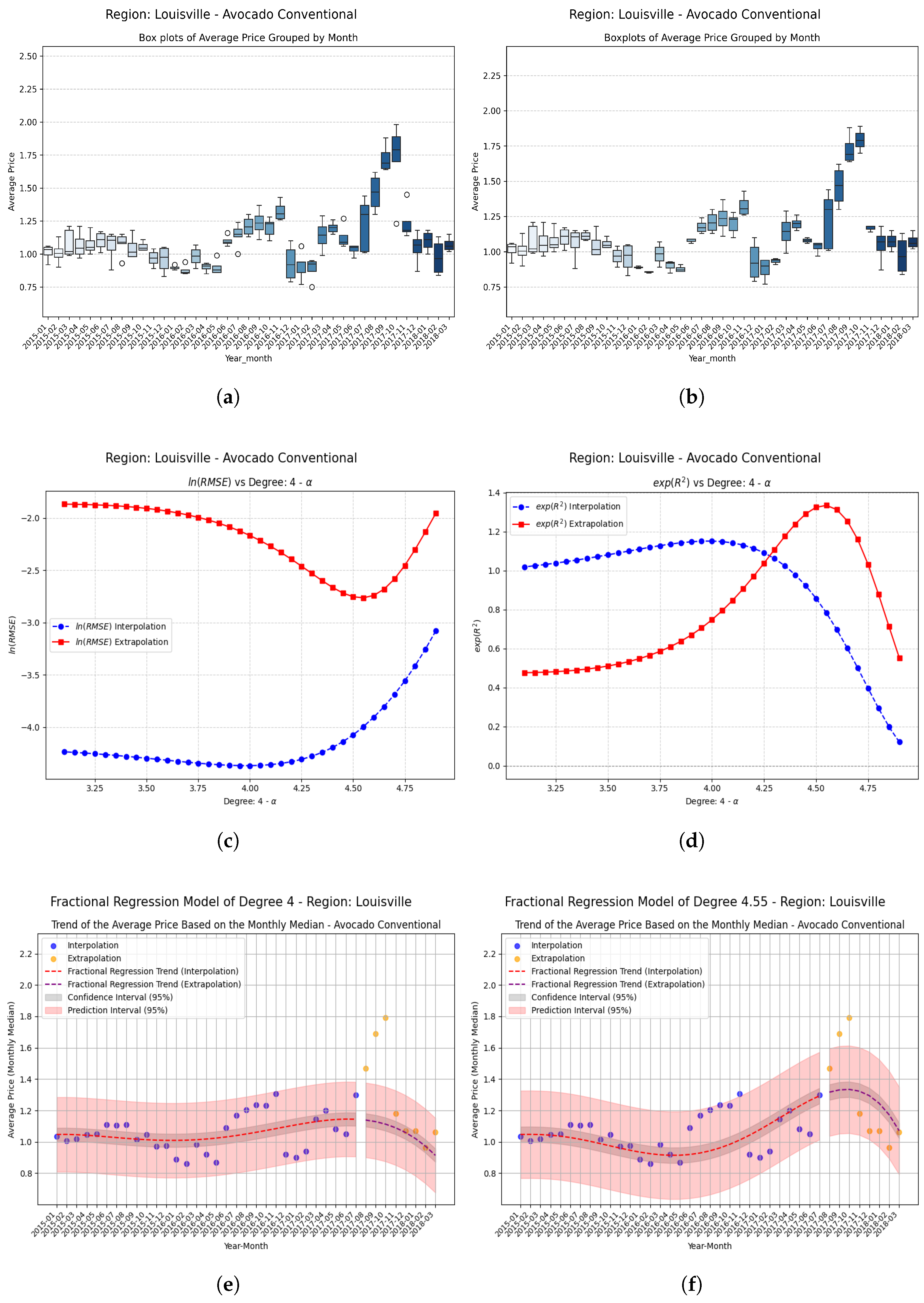
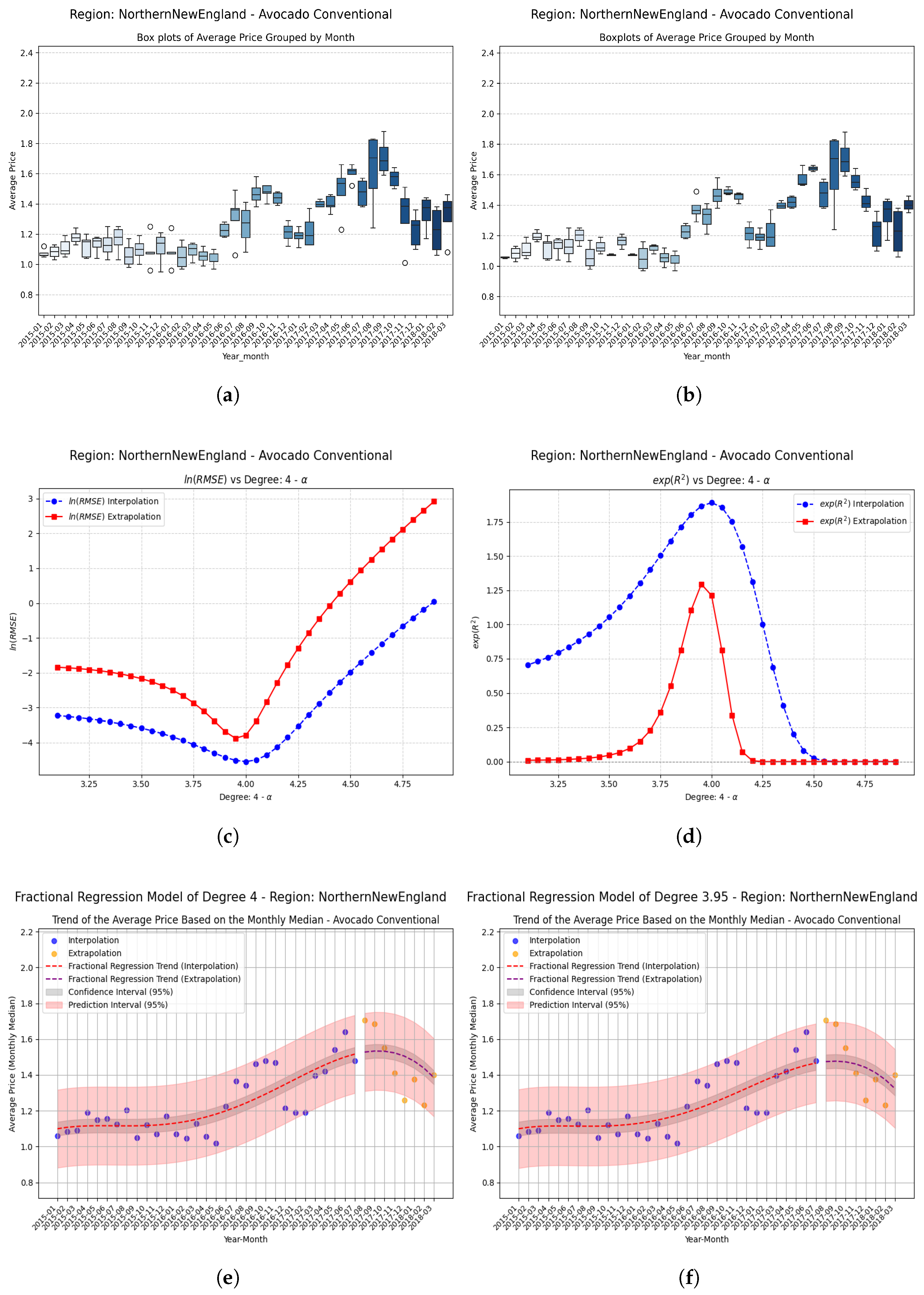
Examples Using Fractional Regression Model
- Interpolation set: Comprises 80% of the data.
- Extrapolation set: Comprises the remaining 20%.
- X: Input features (time or date values).
- y_price: Average price of conventional avocados.
- test_size = 0.2: Proportion allocated for extrapolation.
- random_state = 42: Seed for reproducibility.
- shuffle = False: Maintains temporal order by avoiding data shuffling.
8. Conclusions
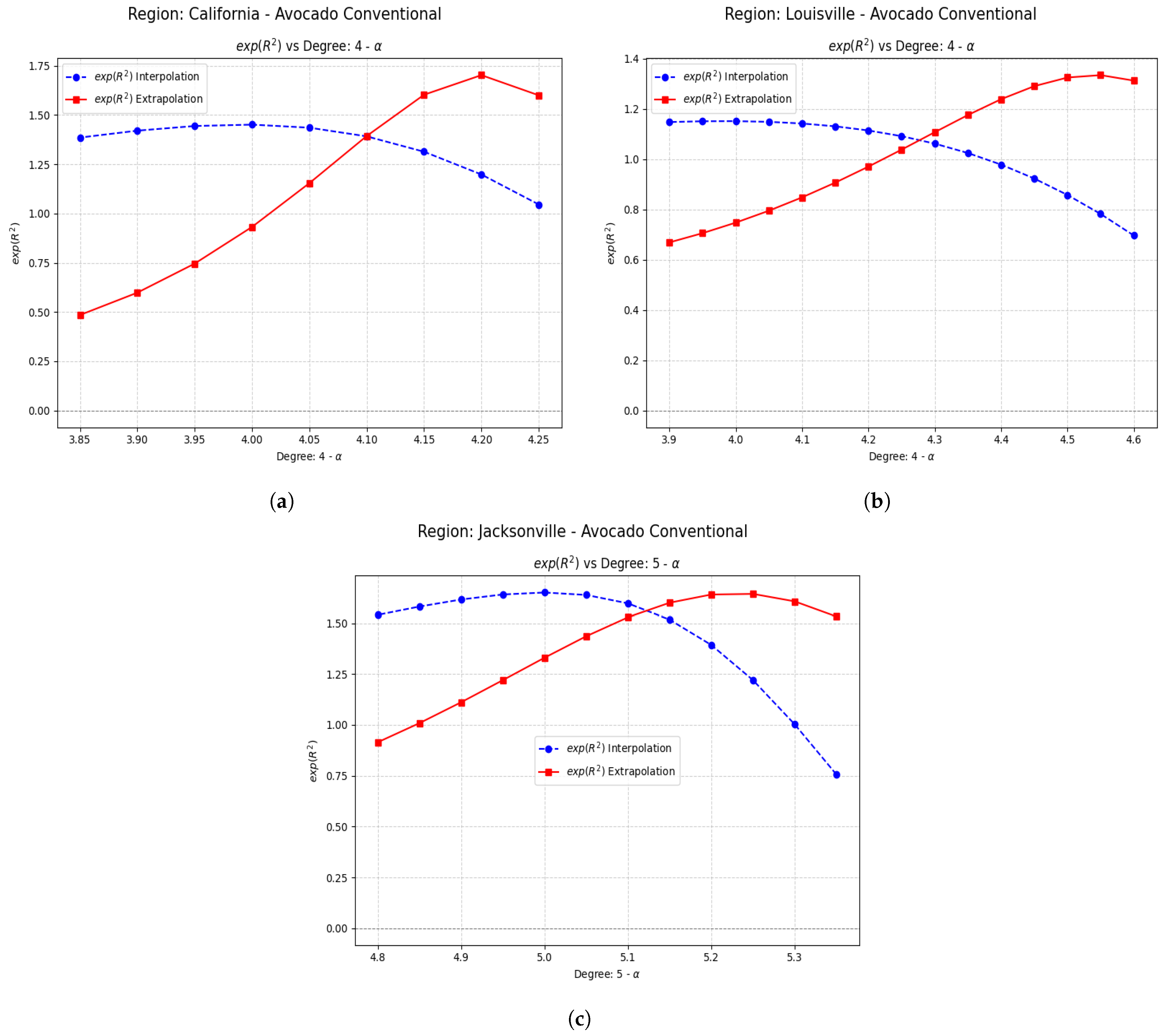
- Regions with initial values that are negative or close to zero exhibit extraordinary improvements after applying the fractional operator. Notable cases include South Carolina, Hartford Springfield, and California, where absolute relative increases exceed on unseen data.
- Regions that start with relatively high and positive coefficients show more modest but consistent improvements, confirming that the technique adds value even where the base model already performs reasonably well.
- Small changes in the parameter can produce large relative improvements, especially in regions with poor initial performance, highlighting the sensitivity and fine-tuning potential of fractional models.
- These results suggest that the proposed approach contributes to overcoming the classical limitations of polynomial models, mainly by increasing the coefficient of determination in unseen data and allowing the generalization of the methods through the implementation of fractional operators, thereby reinforcing the practical applicability of the methodology in predictive analyses based on time series.
Author Contributions
Funding
Data Availability Statement
Conflicts of Interest
References
- Miller, K.S.; Ross, B. An Introduction to the Fractional Calculus and Fractional Differential Equations; Wiley-Interscience: Hoboken, NJ, USA, 1993. [Google Scholar]
- Ross, B. The development of fractional calculus 1695–1900. Hist. Math. 1977, 4, 75–89. [Google Scholar] [CrossRef]
- Hilfer, R. Applications of Fractional Calculus in Physics; World Scientific: Singapore, 2000. [Google Scholar]
- Oldham, K.; Spanier, J. The Fractional Calculus Theory and Applications of Differentiation and Integration to Arbitrary Order; Elsevier: Amsterdam, The Netherlands, 1974; Volume 111. [Google Scholar]
- Kilbas, A.A.; Srivastava, H.M.; Trujillo, J.J. Theory and Applications of Fractional Differential Equations; Elsevier: Amsterdam, The Netherlands, 2006. [Google Scholar]
- De Oliveira, E.C.; Machado, J.A.T. A review of definitions for fractional derivatives and integral. Math. Probl. Eng. 2014, 2014, 1–7. [Google Scholar] [CrossRef]
- Teodoro, G.S.; Machado, J.A.T.; De Oliveira, E.C. A review of definitions of fractional derivatives and other operators. J. Comput. Phys. 2019, 388, 195–208. [Google Scholar] [CrossRef]
- Valério, D.; Ortigueira, M.D.; Lopes, A.M. How many fractional derivatives are there? Mathematics 2022, 10, 737. [Google Scholar] [CrossRef]
- Safdari-Vaighani, A.; Heryudono, A.; Larsson, E. A radial basis function partition of unity collocation method for convection–diffusion equations arising in financial applications. J. Sci. Comput. 2015, 64, 341–367. [Google Scholar] [CrossRef]
- Traore, A.; Sene, N. Model of economic growth in the context of fractional derivative. Alex. Eng. J. 2020, 59, 4843–4850. [Google Scholar] [CrossRef]
- Tejado, I.; Pérez, E.; Valério, D. Fractional calculus in economic growth modelling of the group of seven. Fract. Calc. Appl. Anal. 2019, 22, 139–157. [Google Scholar] [CrossRef]
- Guariglia, E. Fractional calculus, zeta functions and shannon entropy. Open Math. 2021, 19, 87–100. [Google Scholar] [CrossRef]
- Torres-Hernandez, A.; Brambila-Paz, F.; Rodrigo, P.M.; De-la-Vega, E. Reduction of a nonlinear system and its numerical solution using a fractional iterative method. J. Math. Stat. Sci. 2020, 6, 285–299. [Google Scholar]
- Torres-Hernandez, A.; Brambila-Paz, F. Fractional Newton-Raphson Method. Appl. Math. Sci. Int. J. (MathSJ) 2021, 8, 1–13. [Google Scholar] [CrossRef]
- Freitas, F.D.; de Oliveira, L.N. A fractional order derivative newton-raphson method for the computation of the power flow problem solution in energy systems. Fract. Calc. Appl. Anal. 2024, 27, 3414–3445. [Google Scholar] [CrossRef]
- Osler, T.J. Leibniz rule for fractional derivatives generalized and an application to infinite series. SIAM J. Appl. Math. 1970, 18, 658–674. [Google Scholar] [CrossRef]
- Almeida, R. A caputo fractional derivative of a function with respect to another function. Commun. Nonlinear Sci. Numer. Simul. 2017, 44, 460–481. [Google Scholar] [CrossRef]
- Fu, H.; Wu, G.; Yang, G.; Huang, L.-L. Continuous time random walk to a general fractional fokker–planck equation on fractal media. Eur. Phys. J. Spec. Top. 2021, 230, 3927–3933. [Google Scholar] [CrossRef]
- Fan, Q.; Wu, G.-C.; Fu, H. A note on function space and boundedness of the general fractional integral in continuous time random walk. J. Nonlinear Math. Phys. 2022, 29, 95–102. [Google Scholar] [CrossRef]
- Abu-Shady, M.; Kaabar, M.K. A generalized definition of the fractional derivative with applications. Math. Probl. Eng. 2021, 2021, 9444803. [Google Scholar] [CrossRef]
- Saad, K.M. New fractional derivative with non-singular kernel for deriving legendre spectral collocation method. Alex. Eng. J. 2020, 59, 1909–1917. [Google Scholar] [CrossRef]
- Rahmat, M.R.S. A new definition of conformable fractional derivative on arbitrary time scales. Adv. Differ. Equ. 2019, 2019, 1–16. [Google Scholar]
- da C Sousa, J.V.; De Oliveira, E.C. On the ψ-hilfer fractional derivative. Commun. Nonlinear Sci. Numer. Simul. 2018, 60, 72–91. [Google Scholar] [CrossRef]
- Jarad, F.; Uğurlu, E.; Abdeljawad, T.; Baleanu, D. On a new class of fractional operators. Adv. Differ. Equ. 2017, 2017, 1–16. [Google Scholar] [CrossRef]
- Atangana, A.; Gómez-Aguilar, J.F. A new derivative with normal distribution kernel: Theory, methods and applications. Phys. A Stat. Mech. Its Appl. 2017, 476, 1–14. [Google Scholar] [CrossRef]
- Yavuz, M.; Özdemir, N. Comparing the new fractional derivative operators involving exponential and mittag-leffler kernel. Discret. Contin. Dyn. Syst.-S 2020, 13, 995. [Google Scholar] [CrossRef]
- Liu, J.-G.; Yang, X.-J.; Feng, Y.-Y.; Cui, P. New fractional derivative with sigmoid function as the kernel and its models. Chin. J. Phys. 2020, 68, 533–541. [Google Scholar] [CrossRef]
- Yang, X.-J.; Machado, J.A.T. A new fractional operator of variable order: Application in the description of anomalous diffusion. Phys. A Stat. Mech. Its Appl. 2017, 481, 276–283. [Google Scholar] [CrossRef]
- Atangana, A. On the new fractional derivative and application to nonlinear fisher’s reaction–diffusion equation. Appl. Math. Comput. 2016, 273, 948–956. [Google Scholar] [CrossRef]
- He, J.-H.; Li, Z.-B.; Wang, Q.-L. A new fractional derivative and its application to explanation of polar bear hairs. J. King Saud Univ.-Sci. 2016, 28, 190–192. [Google Scholar] [CrossRef]
- Sene, N. Fractional diffusion equation with new fractional operator. Alex. Eng. J. 2020, 59, 2921–2926. [Google Scholar] [CrossRef]
- Torres-Hernandez, A.; Brambila-Paz, F. Sets of fractional operators and numerical estimation of the order of convergence of a family of fractional fixed-point methods. Fractal Fract. 2021, 5, 240. [Google Scholar] [CrossRef]
- Torres-Hernandez, A.; Brambila-Paz, F.; Montufar-Chaveznava, R. Acceleration of the order of convergence of a family of fractional fixed point methods and its implementation in the solution of a nonlinear algebraic system related to hybrid solar receivers. Appl. Math. Comput. 2022, 429, 127231. [Google Scholar] [CrossRef]
- Torres-Hernandez, A.; Brambila-Paz, F.; Ramirez-Melendez, R. Abelian groups of fractional operators. Comput. Sci. Math. Forum 2022, 4, 4. [Google Scholar] [CrossRef]
- Torres-Hernandez, A. Code of a multidimensional fractional quasi-Newton method with an order of convergence at least quadratic using recursive programming. Appl. Math. Sci. Int. J. (MathSJ) 2022, 9, 17–24. [Google Scholar] [CrossRef]
- Trabandt, M.; Uhlig, H. The Laffer curve revisited. J. Monet. Econ. 2011, 58, 305–327. [Google Scholar] [CrossRef]
- Serway, R.A.; Jewett, J.W. Physics for Scientists and Engineers with Modern Physics, 10th ed.; Cengage Learning: Boston, MA, USA, 2018. [Google Scholar]
- Callister, W.D.; Rethwisch, D.G. Materials Science and Engineering: An Introduction, 10th ed.; Wiley: Hoboken, NJ, USA, 2020. [Google Scholar]
- Torres-Hernandez, A.; Brambila-Paz, F.; Torres-Martínez, C. Numerical solution using radial basis functions for multidimensional fractional partial differential equations of type black–scholes. Comput. Appl. Math. 2021, 40, 245. [Google Scholar] [CrossRef]
- Torres-Hernandez, A.; Brambila-Paz, F.; Ramirez-Melendez, R. Proposal for use of the fractional derivative of radial functions in interpolation problems. Fractal Fract. 2023, 8, 16. [Google Scholar] [CrossRef]
- Royston, P.; Altman, D.G. Regression using fractional polynomials of continuous covariates: Parsimonious parametric modelling. J. R. Stat. Soc. Ser. C (Appl. Stat.) 1994, 43, 429–453. [Google Scholar] [CrossRef]
- Awadalla, M.; Noupoue, Y.Y.Y.; Tandogdu, Y.; Abuasbeh, K. Regression Coefficient Derivation via Fractional Calculus Framework. J. Math. 2022, 2022, 1144296. [Google Scholar] [CrossRef]


| Region | Absolute Difference | Absolute Relative Increase | |||
|---|---|---|---|---|---|
| BaltimoreWashington | +0.05 | 0.670462 | 0.704112 | 0.033650 | 0.0502 (5.02%) |
| Chicago | −0.15 | −0.263375 | 0.202223 | 0.465598 | 1.767 (176.7%) |
| HartfordSpringfield | +0.15 | 0.060748 | 0.565226 | 0.504478 | 8.31 (831%) |
| Midsouth | −0.10 | 0.291076 | 0.333769 | 0.042693 | 0.1467 (14.7%) |
| California | −0.20 | −0.070536 | 0.532053 | 0.602589 | 8.54 (854%) |
| GrandRapids | −0.05 | 0.309643 | 0.324153 | 0.01451 | 0.0469 (4.69%) |
| Louisville | −0.55 | −0.290752 | 0.288720 | 0.579472 | 1.993 (199.3%) |
| NorthernNewEngland | +0.05 | 0.192293 | 0.258411 | 0.066118 | 0.3439 (34.4%) |
| Plains | −0.05 | 0.268231 | 0.341435 | 0.073204 | 0.2729 (27.3%) |
| TotalUS | −0.15 | 0.261490 | 0.405492 | 0.144002 | 0.5509 (55.1%) |
| Boise | −0.10 | 0.119390 | 0.274019 | 0.154629 | 1.2947 (129.5%) |
| Jacksonville | −0.25 | 0.285206 | 0.496305 | 0.211099 | 0.7404 (74.0%) |
| SouthCarolina | −0.10 | 0.032100 | 0.397166 | 0.365066 | 11.371 (1137%) |
Disclaimer/Publisher’s Note: The statements, opinions and data contained in all publications are solely those of the individual author(s) and contributor(s) and not of MDPI and/or the editor(s). MDPI and/or the editor(s) disclaim responsibility for any injury to people or property resulting from any ideas, methods, instructions or products referred to in the content. |
© 2025 by the authors. Licensee MDPI, Basel, Switzerland. This article is an open access article distributed under the terms and conditions of the Creative Commons Attribution (CC BY) license (https://creativecommons.org/licenses/by/4.0/).
Share and Cite
Torres-Hernandez, A.; Ramirez-Melendez, R.; Brambila-Paz, F. Proposal for the Application of Fractional Operators in Polynomial Regression Models to Enhance the Determination Coefficient R2 on Unseen Data. Fractal Fract. 2025, 9, 393. https://doi.org/10.3390/fractalfract9060393
Torres-Hernandez A, Ramirez-Melendez R, Brambila-Paz F. Proposal for the Application of Fractional Operators in Polynomial Regression Models to Enhance the Determination Coefficient R2 on Unseen Data. Fractal and Fractional. 2025; 9(6):393. https://doi.org/10.3390/fractalfract9060393
Chicago/Turabian StyleTorres-Hernandez, Anthony, Rafael Ramirez-Melendez, and Fernando Brambila-Paz. 2025. "Proposal for the Application of Fractional Operators in Polynomial Regression Models to Enhance the Determination Coefficient R2 on Unseen Data" Fractal and Fractional 9, no. 6: 393. https://doi.org/10.3390/fractalfract9060393
APA StyleTorres-Hernandez, A., Ramirez-Melendez, R., & Brambila-Paz, F. (2025). Proposal for the Application of Fractional Operators in Polynomial Regression Models to Enhance the Determination Coefficient R2 on Unseen Data. Fractal and Fractional, 9(6), 393. https://doi.org/10.3390/fractalfract9060393