Article

Quasi-Mittag-Leffler Projective Synchronization of Delayed Chaotic Fractional Order Neural Network with Mismatched Parameters

1
School of Mathematics and Information Science, Yantai University, Yantai 264005, China
2
School of Science, Jiangnan University, Wuxi 214122, China
*
Author to whom correspondence should be addressed.
Fractal Fract. 2025, 9(6), 379; https://doi.org/10.3390/fractalfract9060379
Submission received: 18 April 2025 / Revised: 6 June 2025 / Accepted: 12 June 2025 / Published: 15 June 2025
(This article belongs to the Special Issue Analysis and Modeling of Fractional-Order Dynamical Networks)

Abstract

This paper investigates the synchronization control problem for delayed fractional-order neural networks (DFONNs) with mismatched parameters. A novel synchronization behavior termed quasi-Mittag-Leffler projective synchronization (QMLPS) is studied. The core contribution of this work lies in the following: (1) The time delay and mismatched parameters between driven and response systems are considered, which is more general. Both static controllers and adaptive controllers are designed to synchronize the DFONNs. (2) The synchronization errors are estimated, and the rate of convergence is clarified description. By using the Lyapunov stability theory and some significant fractional-order differential inequalities, some sufficient conditions for DFONNs are derived under two kinds of control methods; furthermore, the bound of synchronization errors is estimated by the Mittag-Leffler function. Quantitative numerical simulations have demonstrated the superiority of our controller. Compared to existing results, the QMLPS introduced in this paper is more general, incorporating many existing synchronization concepts. The numerical simulation section verifies the effectiveness of the theoretical results, providing several types of synchronization behaviors of the controlled system under both mismatched and matched parameter conditions, and it also demonstrates the accuracy of the theoretical estimation of synchronization error bounds.

1. Introduction

The synchronization of chaotic systems has received extensive attention due to its important applications, such as secure communication [1,2], dynamics of neuron [3,4,5], etc. Among diverse synchronization behaviors, projective synchronization (PS) constitutes a fundamental phenomenon in the chaotic systems [6], where the trajectories of the systems asymptotically approach each other while one system is a scaled version of the other. There are also some applications of projective synchronization such as secure communication [7,8], image encryption [9,10], etc.
Recent years have witnessed rapidly growing interest in fractional-order systems [11], which exhibit unique dynamic behaviors and offer more accurate representations of real-world processes, especially those involving memory effects, such as epidemic models [12], neuron models [13], lithium-ion batteries [14], etc. The dynamic and chaotic behavior of fractional-order neural networks (FONNs) has been first studied in [15]. Subsequent studies have generated substantial progress in delayed fractional-order neural networks (DFONNs)’ dynamics [16,17,18]. This foundation naturally stimulated extensive synchronization research for DFONNs.
The synchronization of DFONNs was natural for obtaining a lot of results. The synchronization problem of DFONNs has been investigated in [19], in which the Mittag-Leffler function has been applied to design the linear feedback controllers. By using dynamic-free adaptive sliding mode control approach, the synchronization of a specific class of DFONNs with input saturation was discussed in [20]. The distributed impulsive controllers have been designed to synchronize the DFONNs with reaction–diffusion in [21]. Finite-time Mittag-Leffler synchronization for memristive-based DFONNs with uncertainties and perturbations has been researched in [22]. The projective synchronization of FONNs has been first studied in [23]. There are also several important results about projective synchronization for DFONNs. By building an extended fractional-order Halanay inequality, [24] analyzed the projective synchronization of DFONNs with mixed time delays. In [25], global projective synchronization in memristor-based DFONNs was analyzed using a hybrid control methodology that integrates open-loop control with time-delayed feedback control.
We note that the driven and response DFONNs are identical, i.e., they have matched parameters in the above papers. However, mismatched parameters are often unavoidable in real-world systems. Consequently, quasi-synchronization behaviors have garnered significant attention, where the synchronization errors remain bounded rather than converging to zero asymptotically. Recently, few results about the quasi-projective synchronization of discrete-time DFONNs with mismatched parameters have been published recently [26,27,28]. For continuous time DFONNs, quasi-projective synchronization for complex-valued DFONNs have been studied in [29,30,31]; however, the rate of convergence of synchronization errors has not been given in these results.
Based on the preceding discussion, this paper will introduce the concept of quasi-Mittag-Leffler projective synchronization (QMLPS) for DFONNs with mismatched parameters. Specifically, the synchronization error will converge to a bounded closed sphere at the speed of the Mittag-Leffler function. The main contributions of this paper are as follows:
(1)
Incorporation of time delays and mismatched parameters between the driven and response systems, enhancing generality;
(2)
Design of both static and adaptive controllers to achieve synchronization in the DFONNs;
(3)
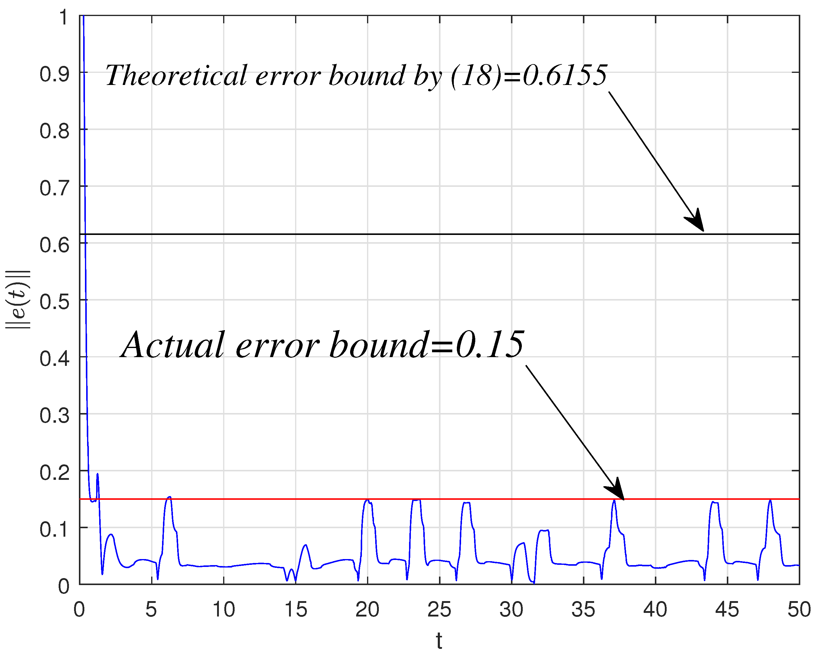
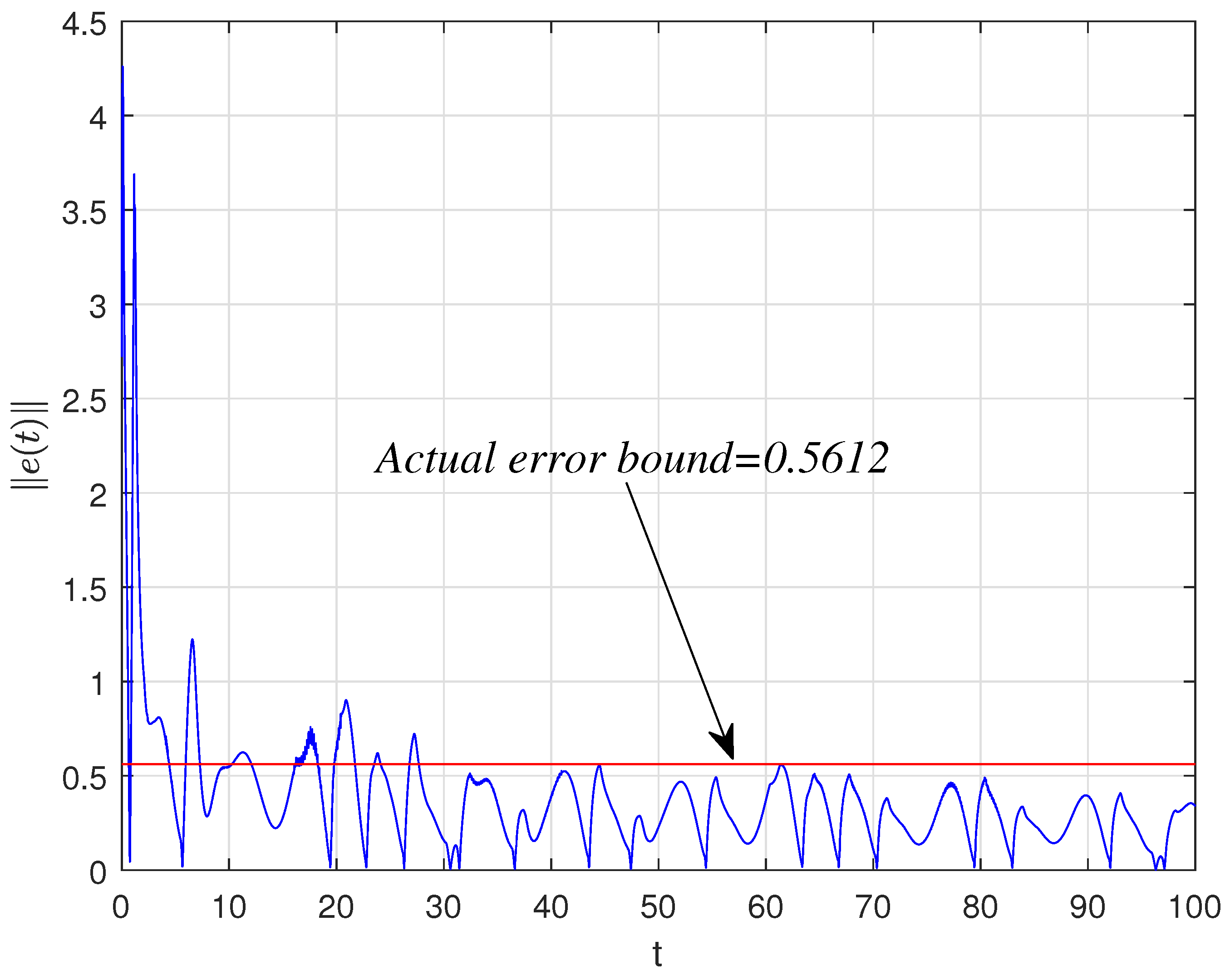
Estimation of synchronization error bounds and explicit characterization of the convergence rate.
The remainder of the paper is structured as follows: Section 2 introduces the mathematical model of delayed chaotic fractional-order neural networks with mismatched parameters and outlines the core problem addressed in this work. Section 3 presents the synchronization scheme and establishes the necessary conditions for achieving QMLPS. Section 4 provides two numerical simulations with matched parameters and mismatched parameters. Finally, the conclusion is drawn.

2. Preliminaries and Problem Formulation

This section covers fractional derivatives fundamentals, the Mittag-Leffler function and its properties, relevant models, essential assumptions, and supporting lemmas.

2.1. Preliminaries of Fractional Order Calculus

 Definition 1. 
The fractional integral operator of order α ( 0 , 1 ) , acting on a function Φ: [ a , b ] R , is given as follows:
a I t α Φ ( t ) = 1 Γ ( α ) a t ( t τ ) α 1 Φ ( τ ) d τ ,
where Γ is the gamma function.
 Definition 2. 
The Caputo fractional derivative of order α ( 0 , 1 ) for a differentiable function Φ: [ a , b ] R is given as follows:
t 0 C D t α Φ ( t ) = 1 Γ ( 1 α ) t 0 t Φ ˙ ( τ ) ( t τ ) α d τ ,
where Γ is the gamma function.
The Mittag-Leffler function is fundamental to fractional-order differential equations, both theoretically and computationally. Its definition and core properties follow.
 Definition 3. 
The two-parameter Mittag-Leffler function is denoted as
E α , β ( z ) = k = 0 z k Γ ( α k + β ) ,
where α > 0 , β > 0 , z C .
For β = 1 , its one-parameter form is
E α = k = 0 z k Γ ( α k + 1 ) = E α , 1 ( z ) .

2.2. System Model and Problem Formulation

Consider the following delayed fractional-order neural network system with n neurons, the dynamics of the ith neuron is described as follows ( i = 1 , 2 , , n )
D t α 0 x i ( t ) = a i x x i ( t ) + j = 1 n b i j x f j ( x i ( t ) ) + j = 1 n c i j x g j ( x i ( t τ ( t ) ) ) + I i ( t ) , t > 0 , x i ( s ) = ϕ i x ( s ) , τ max s 0 ,
which is equivalent to
D t α 0 x ( t ) = A x x ( t ) + B x f ( x ( t ) ) + C x g ( x ( t τ ( t ) ) ) + I ( t ) , t > 0 , x ( s ) = ϕ x ( s ) , τ max s 0 ,
where x i ( t ) denotes the state of the ith neuron, a i x is the rate of return to resting state of the ith neuron, b i j x and c i j x are connection weights on the ith neuron, I i ( t ) is external input of the ith neuron, f i ( · ) and g i ( · ) are activation functions of the ith neuron, i = 1 , 2 , , n . x ( t ) = [ x 1 ( t ) , x 2 ( t ) , , x n ( t ) ] T , A x = diag { a 1 x , a 2 x , , a n x } , B x = b i j x n × n , C x = c i j x n × n , and I ( t ) = [ I 1 ( t ) , I 2 ( t ) , , I n ( t ) ] T . Indeed, the model (4) is the abstract fractional-order Hopfield neural network, which has been shown in the form of an analog circuit in the [32]. The dynamics of ith neuron of the response FONN system is ( i = 1 , 2 , , n )
D t α 0 y i ( t ) = a i y y i ( t ) + j = 1 n b i j y f j ( y i ( t ) ) + j = 1 n c i j y g j ( y i ( t τ ( t ) ) ) + I i ( t ) + u i ( t ) , t > 0 , y i ( s ) = ϕ i y ( s ) , τ max s 0 ,
which is equivalent to
D t α 0 y ( t ) = A y y ( t ) + B y f ( y ( t ) ) + C y g ( y ( t τ ( t ) ) ) + I ( t ) + u ( t ) , t > 0 , y ( s ) = ϕ y ( s ) , τ max s 0 .
where y i ( t ) denotes the state of the ith neuron of the response system, a i y , b i j y and c i j y are similar to the parameters of the (4), u i ( t ) is the controller which will be designed later, and i = 1 , 2 , , n . y ( t ) = [ y 1 ( t ) , y 2 ( t ) , , y n ( t ) ] T , A y = diag { a 1 y , a 2 y , , a n y } , B y = b i j y n × n , C y = c i j y n × n , u ( t ) = [ u 1 ( t ) , u 2 ( t ) , , u n ( t ) ] T .
 Assumption 1. 
The nonlinear functions f ( · ) and g ( · ) satisfy the Lipschitz condition, i.e., there exist constants L f 0 and L g 0 such that
f ( x ) f ( y ) L f x y , g ( x ) g ( y ) L g x y , x , y R n .
 Assumption 2. 
The drive neural network system is bounded, i.e., there exist constants T and ϱ such that
x ( t ) ϱ , t T .
 Remark 1. 
The above two assumptions are mild. Firstly, the Lipschitz condition is a common constraint to ensure the existence uniqueness of solution. Secondly, many systems are bounded, such as chaotic systems, periodic orbit, etc. Indeed, some related papers assumed f ( x ) f ( p y ) L f x p y to deal with the projective problem [33]; it is obviously a higher demand for the systems.
Denote the projective synchronization error as e i ( t ) = y i ( t ) p x i ( t ) ( i = 1 , 2 , , n ) ; the parameter p is a so-called “scaling factor”. Then, one has the following dynamics for the errors ( i = 1 , 2 , , n )
D t α 0 e i ( t ) = a i y e i ( t ) + j = 1 n b i j y f ˜ j ( t ) + j = 1 n c i j y g ˜ j ( t τ ( t ) ) + δ i ( t ) + θ i ( t ) + u i ( t ) , t > 0 , e i ( s ) = ϕ i ( s ) = ϕ i y ( s ) p ϕ i x ( s ) , τ max s 0 ,
where
δ i ( x ( t ) ) = ( a i y p a i x ) x i ( t ) + j = 1 n ( b i j y b i j x ) f j ( p x ( t ) ) + j = 1 n ( c i j y c i j x ) g j ( p x ( t τ ( t ) ) ) ,
θ i ( x ( t ) , x ( t τ ( t ) ) ) = j = 1 n b i j x ( f j ( p x ( t ) ) p f j ( x ( t ) ) ) + j = 1 n c i j x ( g j ( p x ( t τ ) ) p g j ( x ( t τ ) ) ) ,
f ˜ i ( t ) = f i ( y ( t ) ) f i ( p x ( t ) ) , g ˜ i ( t τ ( t ) ) = g i ( y ( t τ ( t ) ) ) g i ( p x ( t τ ( t ) ) ) ,
which is equivalent to
D t α 0 e ( t ) = A y e ( t ) + B y f ˜ ( t ) + C y g ˜ ( t τ ( t ) ) + δ ( t ) + θ ( t ) + u ( t ) , t > 0 , e i ( s ) = ϕ ( s ) , τ max s 0 ,
where e ( t ) = [ e 1 ( t ) , e 2 ( t ) , , e n ( t ) ] T R n denotes the PS error vector. Some vectors symbols are defined as follows: f ˜ ( t ) = [ f ˜ 1 ( · ) , f ˜ 2 ( · ) , , f ˜ n ( · ) ] T , g ˜ ( t τ ( t ) ) = [ g ˜ 1 ( · ) , g ˜ 2 ( · ) , , g ˜ n ( · ) ] T , θ ( t ) = [ θ 1 ( · ) , θ 2 ( · ) , , θ n ( · ) ] T , δ ( t ) = [ δ 1 ( · ) , δ 2 ( · ) , , δ n ( · ) ] T .
 Remark 2. 
According to the Assumption 2 and the continuity of functions f ( · ) and g ( · ) , one can conclude that θ i ( · ) and δ i ( · ) are also bounded, i.e., there exist constants θ ^ i 0 and δ ^ i 0 such that θ i ( · )   θ ^ i and δ i ( · )   δ ^ i for all t T , i = 1 , 2 , , n .
It is easy to see that the PS between (4) and (6) is equivalent to lim t + e ( t ) = 0 . However, the parameters are mismatched between the drive system and response system, thus, it will be difficult to achieve complete PS under the linear feedback controllers, and the following quasi-PS is more suitable for this case.
 Definition 4. 
The drive system (4) and the response system (6) achieve quasi-projective synchronization (quasi-PS) with error bound ϵ > 0 for all initial conditions e ( s ) , and where τ max s 0 , the error signal e ( t ) converges into the set
M = { e ( t ) e ( t ) ϵ } .
Furthermore, we often need to estimate the rate of convergence of the synchronization behavior, and the following definition, named “quasi-MLPS (quasi-Mittag Leffler projective synchronization)” based on the Mittag-Leffler function, will be used in this paper.
 Definition 5. 
The drive system (4) and the response system (6) achieve quasi-MLPS with an error bounded ϵ > 0 and convergent rate r > 0 if for any initial values satisfied e ( s ) ( τ max s 0 ) , there exist constants M > 0 , b > 0 , and t m > 0 , such that for any t t m , the error signal e ( t ) satisfies
e ( t ) { M E α ( r t α ) } b + ϵ .
 Remark 3. 
Noting that when ϵ = 0 and p = 1 , the quasi-MLPS becomes the classical Mittag–Leffler synchronization. Furthermore, when α = 1 and ϵ = 0 , it will be exponential projective synchronization. Thus, the above quasi-MLPS has included a lot of kinds of synchronization behaviors.
 Lemma 1 
(Fractional Halanay Inequality, [34]). Assume that the function w ( t ) 0 and satisfies
D t α 0 w ( t ) = γ 1 w ( t ) + γ 2 max t τ ( t ) s t w ( s ) + γ 3 , t > 0 , w ( s ) = ϕ ( s ) , τ max s 0 ,
where constants γ 2 0 , γ 3 0 and γ 1 + γ 2 0 , 0 τ ( t ) τ m . Then there exists M such that
w ( t ) M E α ( λ ¯ t α ) γ 3 γ 1 + γ 2 ,
for any t τ ( t ) + 1 , where
λ ¯ = sup t τ ( t ) 1 λ λ γ 1 γ 2 E α ( λ ( t τ ( t ) ) α ) E α ( λ t α ) = 0 .
 Lemma 2 
([26]). Let v 1 ( t ) 0 be continuous on [ 0 , + ) and bounded on [ τ m , 0 ) ; v 2 ( t ) 0 is continuous on [ 0 , + ) , which satisfies
D t α 0 ( v 1 ( t ) + v 2 ( t ) ) q 1 v 1 ( t ) + q 2 sup t τ m s t v 1 ( s ) + q 3 ,
where 0 < α < 1 , q 1 > q 2 > 0 , q 3 0 ; then, for any given M 0 > 0 , there exists T > 0 such that
v 1 ( t ) v 1 ( 0 ) + v 2 ( 0 ) q 3 q 1 E α ( q 1 t α ) + q 3 q 1 1 q 2 q 1 + M 0 , t > T .

3. Main Results

In this section, both static controllers and adaptive controllers are designed, and the conditions to ensure the quasi-PS or quasi-MLPS between (4) and (6) are derived.

3.1. Static Controllers

Consider the following simple static linear feedback controllers
u i ( t ) = d i e i ( t ) , i = 1 , 2 , , n .
 Remark 4. 
In this subsection, the static linear feedback controllers above have been designed, which are independent with the scaling factor p. However, some existing results about projective synchronization have designed controllers with more complex forms; see, for example, [23,24,25].
 Theorem 1. 
Under Assumption 1 and Assumption 2, if there exist matrix P > 0 , constants a > 0 such that
2 A y + P B y ( B y ) T P + L f 2 I n + P C y ( C y ) T P 2 D + a P 0 ,
L g 2 a p m ,
where D = diag { d 1 , d 2 , , d n } , p m > 0 is the smallest eigenvalue of P. Then, the quasi-MLPS can be achieved between (4) and (6) with controllers (10), and the error bound and convergent rate will be given in the proof process.
 Proof. 
Let V 1 ( t ) = e T ( t ) P e ( t ) ; calculating the derivative of V 1 ( t ) along the error system (9), one has
D t α 0 V 1 ( t ) 2 e T ( t ) P 0 D t α e ( t ) = 2 e T ( t ) P A y e ( t ) + B y f ˜ ( t ) + C y g ˜ ( t τ ( t ) ) + δ ( t ) + θ ( t ) D e ( t ) ,
according to the Assumption 1, we have
2 e T ( t ) P B y f ˜ ( t ) e T ( t ) P B y ( B y ) T P e ( t ) + f ˜ T ( t ) f ˜ ( t ) e T ( t ) { P B y ( B y ) T P + L f 2 I n } e ( t ) ,
2 e T ( t ) P C y g ˜ ( t τ ( t ) ) e T ( t ) P C y ( C y ) T P e ( t ) + g ˜ T ( t τ ( t ) ) g ˜ ( t τ ( t ) ) e T ( t ) P C y ( C y ) T P e ( t ) + L g 2 e T ( t τ ( t ) ) e ( t τ ( t ) ) .
Based on the Remark 2, one has
2 e T ( t ) P δ ( t ) e T ( t ) P 2 e ( t ) + δ T ( t ) δ ( t ) e T ( t ) P 2 e ( t ) + δ ˜ ,
2 e T ( t ) P θ ( t ) e T ( t ) P 2 e ( t ) + θ T ( t ) θ ( t ) e T ( t ) P 2 e ( t ) + θ ˜ ,
where δ ˜ = i = 1 n δ ^ i 2 and θ ˜ = i = 1 n θ ^ i 2 . Thus,
D t α 0 V 1 ( t ) e T ( t ) 2 A y + P B y ( B y ) T P + L f 2 I n + P C y ( C y ) T P 2 D e ( t ) + L g 2 e T ( t τ ( t ) ) e ( t τ ( t ) ) + ζ ,
where ζ = δ ˜ + θ ˜ . Then, (11) implies that
D t α 0 V 1 ( t ) a V 1 ( t ) + b V 1 ( t τ ( t ) ) + ζ ,
where b = L g 2 p m . According to the Lemma 1 and (12), there exists M such that
V 1 ( t ) M E α ( r t α ) + ζ a b ,
where
r = sup t τ ( t ) 1 λ λ + a b E α ( λ ( t τ ( t ) ) α ) E α ( λ t α ) = 0 .
Consequently, it is easy to get
e ( t ) { M E α ( r t α ) } 1 2 + ζ a b ,
which implies that the quasi-MLPS can be achieved between the fractional-order neural network (4) and (6) with an error bounded ζ a b and convergent rate r. □

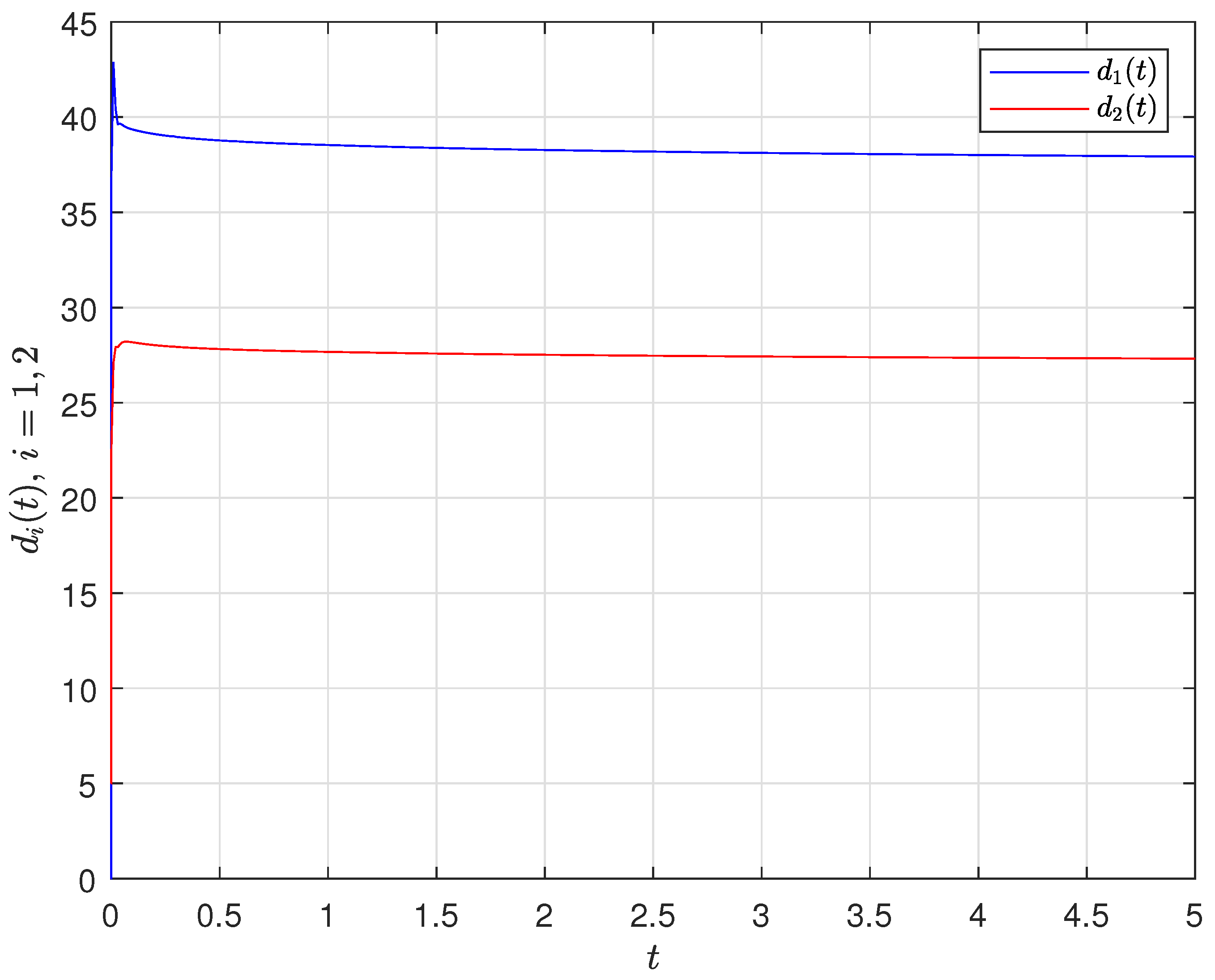
3.2. Adaptive Controllers

In the above subsection, the control gain d i ( i = 1 , 2 , , n ) is required to be large enough to satisfy the condition (11), but it may be much larger than the needed values. In the following, we will apply the adaptive control approach. Consider the following adaptive linear feedback controllers and adaptive law
u i ( t ) = d i ( t ) e i ( t ) , D t α 0 d i ( t ) = β i e i 2 ( t ) ,
where β i are positive constants, i = 1 , 2 , , n .
 Theorem 2. 
Under Assumption 1 and Assumption 2, if there exist matrix P > 0 , constants μ > 0 such that
2 A y + P B y ( B y ) T P + L f 2 I n + P C y ( C y ) T P 2 Ξ + μ P 0 ,
L g 2 < μ ,
where Ξ = diag { σ 1 , σ 2 , , σ n } , σ i > 0 are sufficiently large constants. Then, the quasi-MLPS can be achieved between (4) and (6) with controllers (10), and the error bound and convergent rate will be given in the proof process.
 Proof. 
Let V 21 ( t ) = e T ( t ) P e ( t ) , V 22 ( t ) = i = 1 n ( d i ( t ) σ i ) 2 β i , and V 2 ( t ) = V 21 ( t ) + V 22 ( t ) . Calculating the derivative of V 21 ( t ) along the error system (9), which is similar to the proof of Theorem 1, one has
D t α 0 V 21 ( t ) e T ( t ) 2 A y + P B y ( B y ) T P + L f 2 I n + P C y ( C y ) T P 2 D ( t ) e ( t ) + L g 2 e T ( t τ ( t ) ) e ( t τ ( t ) ) + ζ ,
where D ( t ) = diag { d 1 ( t ) , d 2 ( t ) , , d n ( t ) } and ζ = δ ˜ + θ ˜ . On the other hand, the α-order derivative of V 22 ( t ) is
D t α 0 V 22 ( t ) i = 1 n 2 ( d i ( t ) σ i ) β i · 0 D t α d i ( t ) = e T ( t ) { 2 D ( t ) 2 Ξ } e ( t ) ,
where Ξ = diag { σ 1 , σ 2 , , σ n } . Then, it follows from fractional-order Razumikhin theorem that
D t α 0 V 2 ( t ) = D t α 0 ( V 21 ( t ) + V 22 ( t ) ) e T ( t ) 2 A y + P B y ( B y ) T P + L f 2 I n + P C y ( C y ) T P 2 Ξ e ( t ) + L g 2 e T ( t τ ( t ) ) e ( t τ ( t ) ) + ζ μ V 21 ( t ) + L g 2 sup t τ m s t V 21 ( s ) + ζ ,
and we can choose σ i such that μ L g 2 > 0 . According to the Lemma 2, for any M 0 > 0 , we have
V 21 ( t ) V 21 ( 0 ) + V 22 ( 0 ) ζ μ E α ( μ t α ) + ζ μ 1 L g 2 μ + M 0 .
Consequently, we let M 0 0 , and it is easy to get
e ( t ) { M ˜ E α ( μ t α ) } 1 2 + ζ μ L g 2 ,
where M ˜ = V 21 ( 0 ) + V 22 ( 0 ) ζ μ 1 L g 2 μ , which implies that the quasi-MLPS can be achieved between the fractional-order neural network (4) and (6), with an error bounded ζ μ L g 2 and convergent rate μ. □
 Remark 5. 
By comparing the adaptive controllers (22) and the static feedback controllers (10), it can be observed that the adaptive controllers are easier to implement, requiring only that the parameter β i > 0 , i = 1 , 2 , , n . In contrast, the static feedback controller requires the control gain d i ( i = 1 , 2 , , n ) to be sufficiently large in order to more easily satisfy the desired condition (11) of Theorem 1, thereby achieving a larger μ, which corresponds to a faster convergence rate. However, the adaptive controllers also have certain limitations, primarily related to the steady-state value of the adaptive control gain d i ( t ) , i = 1 , 2 , , n . This paper does not provide a theoretical analysis of the convergence of the adaptive control gain, which is a topic for future investigation. Nevertheless, the simulation results in this paper demonstrate the convergence behavior of d i ( t ) , i = 1 , 2 , , n , indicating that its steady-state value does not show a significant advantage over that of the static feedback control gain.

4. Numerical Simulation

In this section, two examples are given to show the effectiveness of the above theoretical results. The predictor–corrector algorithm has been used to simulate the fractional-order dynamical networks in this paper [35]. The discretization step size is set to 0.005, and all simulations were carried out using MATLAB software, version 2018b. In the system (5), if α = 0.99 , parameters A x , B x , and C x are selected as
A x = 1 0 0 1 , B x = 1 + 0.25 π 20 0.1 1 + 0.25 π , C x = 0.325 2 π 0.1 0.1 0.325 2 π .
And f ( x i ) = g ( x i ) = | x i + 1 | | x i 1 | 2 , τ ( t ) = 1 . When s [ 1 , 0 ] , ϕ x ( s ) = [ 10.1 ] T . Then, the chaotic behavior is shown in Figure 1. Furthermore, one can calculate the L f = L g = 1 in Assumption 1. And x ( t )   ϱ = 13.43 when t 20 .

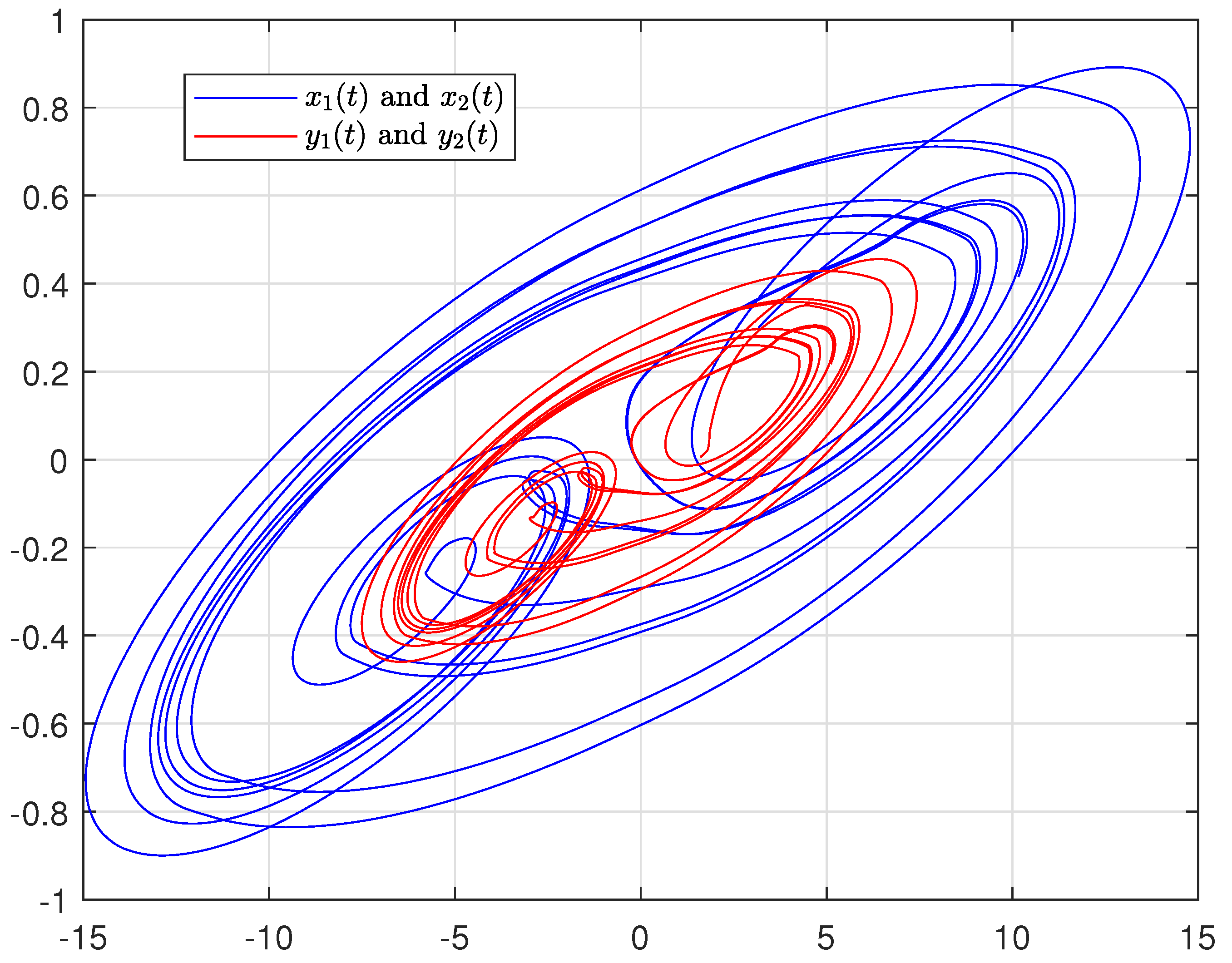
4.1. Synchronization Behaviors with Matched Parameters

If A y = A x , B y = B x , C y = C x , it is easy to see δ i ( x ( t ) ) = 0 , i = 1 , 2 . Letting ϕ y = [ 0.1 , 0.1 ] T when s [ 1 , 0 ] , one can see the differential orbits of the driven system and response system in Figure 2 without control, which is obviously not any synchronization behavior. When we select the “scaling factor” p = 1 , noting that f ( x ) = f ( x ) , one has θ ( x ( t ) , x ( t τ ( t ) ) ) = 0 , i = 1 , 2 . Then, ζ = 0 , i.e., the complete anti-synchronization between (4) and (6) can be achieved when d 1 = d 2 = 10 according to Theorem 1. The complete anti-synchronization state and synchronization error e ( t ) = y ( t ) x ( t ) in this case can be seen in Figure 3 and Figure 4, respectively.
Let “scaling factor” p = 0.5 . According to the simulation results, one can get θ ˜ = θ ^ 1 2 + θ ^ 2 2 = 2.61 . By solving the conditions (11) and (12), we have P = diag { 0.1 , 0.1 } , a = 16.89 , and then b = 10 . According to the (21) of Theorem 1, the error bound ζ a b = 0.6155 . Letting ϕ y = [ 10 , 10 ] T when s [ 1 , 0 ] , one can see the synchronization error e ( t ) in Figure 5. In addition, the synchronization error bound e ( t ) can be seen in Figure 6. Furthermore, the “scaling factor” can be found directly from the chaotic behaviors which are shown in Figure 7. One can also apply the adaptive strategy, let β 1 = 20 , β 2 = 10 , d 1 ( 0 ) = 0 , and d 2 ( 0 ) = 5 , and the synchronization error bound e ( t ) can be seen in Figure 8; the adaptive control gains d 1 ( t ) and d 2 ( t ) are shown in Figure 9. This could verify the results of Theorem 2.

4.2. Synchronization Behaviors with Mismatched Parameters

Let parameters A y , B y , and C y be selected as
A y = 0.1 0 0 0.1 , B x = 1.5 22 1 1.6 , C x = 1.5 0 0 1.5 .
When we select the “scaling factor” p = 1 , one has θ ( x ( t ) , x ( t τ ( t ) ) ) = 0 ; however, δ i ( x ( t ) ) 0 due to the mismatched parameters, i = 1 , 2 . Without any control, the anti-synchronization errors e ( t ) and e ( t ) are shown in Figure 10 and Figure 11, respectively. Let β 1 = 2 , β 2 = 2 , d 1 ( 0 ) = 0 , and d 2 ( 0 ) = 0 ; the quasi-anti synchronization can be achieved according to Theorem 2. The synchronization error bound e ( t ) can be seen in Figure 12, and the adaptive control gains d 1 ( t ) and d 2 ( t ) are shown in Figure 13; the quasi-anti synchronization behaviors can be seen in Figure 14, respectively.

5. Conclusions

The paper investigates the synchronization behavior of delayed fractional-order neural networks (DFONNs), which incorporate time delays, parameter mismatches, and fractional-order dynamics. A novel concept, termed Quasi-Mittag-Leffler Projective Synchronization (QMLPS), is introduced, which encompasses several existing synchronization types as special cases. Initially, static linear feedback controllers are designed, where the control gains are required to satisfy certain conditions. Subsequently, an adaptive control approach is employed to autonomously adjust the control gains. Several numerical examples are presented to validate the proposed control strategies, and the boundedness of the synchronization error is demonstrated through simulation results. In future work, there are two promising directions that can be explored as follows: (1) Extending the current QMLPS framework to more complex network topologies, such as multilayer or stochastic neural networks, which could provide deeper insights into real-world systems. (2) Applying the theoretical results of chaotic synchronization in fractional-order neural network systems to practical problems such as image encryption and secure communication.

Author Contributions

Conceptualization, X.S.; software, X.S.; validation, Y.Y.; writing—original draft preparation, X.S.; writing—review and editing, Y.Y.; supervision, Y.Y.; project administration, X.S.; funding acquisition, Y.Y. All authors have read and agreed to the published version of the manuscript.

Funding

This research is supported by the Doctoral Start-up Fund of Yantai University (No: SX22B06).

Data Availability Statement

The original contributions presented in this study are included in the article. Further inquiries can be directed to the corresponding author.

Acknowledgments

The authors would like to express their sincere gratitude to the reviewers and the editor for their valuable comments and suggestions.

Conflicts of Interest

The authors declare no conflicts of interest.

References

  1. Yang, T. A survey of chaotic secure communication systems. Int. J. Comput. Cogn. 2004, 2, 81–130. [Google Scholar]
  2. Liu, J.; Zhang, J.; Wang, Y. Secure communication via chaotic synchronization based on reservoir computing. IEEE Trans. Neural Netw. Learn. Syst. 2022, 35, 285–299. [Google Scholar] [CrossRef]
  3. Pecora, L.M.; Carroll, T.L. Synchronization in chaotic systems. Phys. Rev. Lett. 1990, 64, 821. [Google Scholar] [CrossRef] [PubMed]
  4. Arecchi, F.T. Chaotic neuron dynamics, synchronization and feature binding. Phys. A Stat. Mech. Its Appl. 2004, 338, 218–237. [Google Scholar] [CrossRef]
  5. Lin, H.; Wang, C.; Deng, Q.; Xu, C.; Deng, Z.; Zhou, C. Review on chaotic dynamics of memristive neuron and neural network. Nonlinear Dyn. 2021, 106, 959–973. [Google Scholar] [CrossRef]
  6. Mainieri, R.; Rehacek, J. Projective synchronization in three-dimensional chaotic systems. Phys. Rev. Lett. 1999, 82, 3042. [Google Scholar] [CrossRef]
  7. Sun, J.; Zang, M.; Wang, Z.; Wang, Y. Coupling projection synchronization of three chaotic systems and its multilevel secure communication via DNA CRNs. IEEE Internet Things J. 2023, 10, 17282–17292. [Google Scholar] [CrossRef]
  8. Li, Z.; Tang, Y.; Xu, F.; Zhang, Y. Full states pseudo-random projective synchronization of hyperchaotic system and corresponding secure communication algorithm. Multimed. Tools Appl. 2024, 84, 3527–3568. [Google Scholar] [CrossRef]
  9. Bharti, J.K.; Balasubramaniam, P.; Murugesan, K. Image encryption algorithm based on matrix projective combination-combination synchronization of an 11-dimensional time delayed hyperchaotic system. Phys. Scr. 2024, 99, 125008. [Google Scholar] [CrossRef]
  10. He, J.; Wu, Y.; Yang, C. Function matrix projective synchronization for disturbed fractional laser chaotic systems and image encryption. Chin. J. Phys. 2025, 95, 1078–1095. [Google Scholar] [CrossRef]
  11. Kothari, K.; Mehta, U.V.; Prasad, R. Fractional-order system modeling and its applications. J. Eng. Sci. Technol. Rev. 2019, 12, 1–10. [Google Scholar] [CrossRef]
  12. Chen, Y.; Liu, F.; Yu, Q.; Li, T. Review of fractional epidemic models. Appl. Math. Model. 2021, 97, 281–307. [Google Scholar] [CrossRef] [PubMed]
  13. Ding, D.; Niu, Y.; Yang, Z.; Wang, J.; Wang, W.; Wang, M.; Jin, F. Extreme multi-stability and microchaos of fractional-order memristive Rulkov neuron model considering magnetic induction and its digital watermarking application. Nonlinear Dyn. 2024, 112, 15523–15545. [Google Scholar] [CrossRef]
  14. Zhang, X.; Gao, X.; Duan, L.; Gong, Q.; Wang, Y.; Ao, X. A novel method for state of health estimation of lithium-ion batteries based on fractional-order differential voltage-capacity curve. Appl. Energy 2025, 377, 124404. [Google Scholar] [CrossRef]
  15. Kaslik, E.; Sivasundaram, S. Nonlinear dynamics and chaos in fractional-order neural networks. Neural Netw. 2012, 32, 245–256. [Google Scholar] [CrossRef] [PubMed]
  16. Wang, F.; Yang, Y.; Hu, M. Asymptotic stability of delayed fractional-order neural networks with impulsive effects. Neurocomputing 2015, 154, 239–244. [Google Scholar] [CrossRef]
  17. Zhang, F.; Huang, T.; Wu, Q.; Zeng, Z. Multistability of delayed fractional-order competitive neural networks. Neural Netw. 2021, 140, 325–335. [Google Scholar] [CrossRef]
  18. Zhang, F.; Huang, T.; Wu, A.; Zeng, Z. Mittag-Leffler stability and application of delayed fractional-order competitive neural networks. Neural Netw. 2024, 179, 106501. [Google Scholar] [CrossRef]
  19. Wang, C.; Yang, Q.; Zhuo, Y.; Li, R. Synchronization analysis of a fractional-order non-autonomous neural network with time delay. Phys. A Stat. Mech. Its Appl. 2020, 549, 124176. [Google Scholar] [CrossRef]
  20. Roohi, M.; Zhang, C.; Taheri, M.; Basse-O’Connor, A. Synchronization of fractional-order delayed neural networks using dynamic-free adaptive sliding mode control. Fractal Fract. 2023, 7, 682. [Google Scholar] [CrossRef]
  21. Liu, F.; Yang, Y.; Chang, Q. Synchronization of fractional-order delayed neural networks with reaction–diffusion terms: Distributed delayed impulsive control. Commun. Nonlinear Sci. Numer. Simul. 2023, 124, 107303. [Google Scholar] [CrossRef]
  22. Fan, H.; Chen, X.; Shi, K.; Liang, Y.; Wang, Y.; Wen, H. Mittag-Leffler synchronization in finite time for uncertain fractional-order multi-delayed memristive neural networks with time-varying perturbations via information feedback. Fractal Fract. 2024, 8, 422. [Google Scholar] [CrossRef]
  23. Yu, J.; Hu, C.; Jiang, H.; Fan, X. Projective synchronization for fractional neural networks. Neural Netw. 2014, 49, 87–95. [Google Scholar] [CrossRef] [PubMed]
  24. Liu, P.; Kong, M.; Zeng, Z. Projective synchronization analysis of fractional-order neural networks with mixed time delays. IEEE Trans. Cybern. 2020, 52, 6798–6808. [Google Scholar] [CrossRef] [PubMed]
  25. Gu, Y.; Yu, Y.; Wang, H. Projective synchronization for fractional-order memristor-based neural networks with time delays. Neural Comput. Appl. 2019, 31, 6039–6054. [Google Scholar] [CrossRef]
  26. Zhang, X.L.; Li, H.L.; Yu, Y.; Zhang, L.; Jiang, H. Quasi-projective and complete synchronization of discrete-time fractional-order delayed neural networks. Neural Netw. 2023, 164, 497–507. [Google Scholar] [CrossRef]
  27. Zhang, H.; Chen, X.; Ye, R.; Stamova, I.; Cao, J. Quasi-projective synchronization analysis of discrete-time FOCVNNs via delay-feedback control. Chaos Solitons Fractals 2023, 173, 113629. [Google Scholar] [CrossRef]
  28. Li, D.D.; Li, H.L.; Hu, C.; Jiang, H.; Cao, J. Projective synchronization of discrete-time variable-order fractional neural networks with time-varying delays. IEEE Trans. Neural Netw. Learn. Syst. 2025, 36, 9313–9325. [Google Scholar] [CrossRef]
  29. Cheng, J.; Zhang, H.; Zhang, W.; Zhang, H. Quasi-projective synchronization for Caputo type fractional-order complex-valued neural networks with mixed delays. Int. J. Control. Autom. Syst. 2022, 20, 1723–1734. [Google Scholar] [CrossRef]
  30. Yan, H.; Qiao, Y.; Duan, L.; Miao, J. New results of quasi-projective synchronization for fractional-order complex-valued neural networks with leakage and discrete delays. Chaos Solitons Fractals 2022, 159, 112121. [Google Scholar] [CrossRef]
  31. Zhu, J.; Zhang, G.; Wang, L. Quasi-projective and finite-time synchronization of fractional-order memristive complex-valued delay neural networks via hybrid control. AIMS Math. 2024, 9, 7627–7644. [Google Scholar] [CrossRef]
  32. Pu, Y.F.; Yi, Z.; Zhou, J.L. Fractional Hopfield neural networks: Fractional dynamic associative recurrent neural networks. IEEE Trans. Neural Netw. Learn. Syst. 2016, 28, 2319–2333. [Google Scholar] [CrossRef] [PubMed]
  33. Ma, T.; Zhang, J.; Zhou, Y.; Wang, H. Adaptive hybrid projective synchronization of two coupled fractional-order complex networks with different sizes. Neurocomputing 2015, 164, 182–189. [Google Scholar] [CrossRef]
  34. Wang, D.; Zou, J. Dissipativity and contractivity analysis for fractional functional differential equations and their numerical approximations. SIAM J. Numer. Anal. 2019, 57, 1445–1470. [Google Scholar] [CrossRef]
  35. Bhalekar, S.; Daftardar, V. A predictor-corrector scheme for solving nonlinear delay differential equations of fractional order. J. Fract. Calc. Appl. 2011, 1, 1–9. [Google Scholar]
Figure 1. Chaotic behavior of the driven system with ϕ x ( s ) = [ 1 , 0.1 ] T , s [ 1 , 0 ] .
Fractalfract 09 00379 g001
Figure 2. x ( t ) and y ( t ) without control.
Fractalfract 09 00379 g002
Figure 3. x ( t ) and y ( t ) under control with d 1 = d 2 = 10 .
Fractalfract 09 00379 g003
Figure 4. Error state e ( t ) under control with d 1 = d 2 = 10 .
Fractalfract 09 00379 g004
Figure 5. Synchronization error e ( t ) without control with ϕ y ( s ) = [ 10 , 10 ] T , s [ 1 , 0 ] .
Fractalfract 09 00379 g005
Figure 6. Synchronization error e ( t ) = y ( t ) 0.5 x ( t ) with controllers (10).
Fractalfract 09 00379 g006
Figure 7. Chaotic behaviors of driven system and response system with controllers (10).
Fractalfract 09 00379 g007
Figure 8. Synchronization error e ( t ) = y ( t ) 0.5 x ( t ) with controllers (22).
Fractalfract 09 00379 g008
Figure 9. Evolution of d 1 ( t ) and d 2 ( t ) .
Fractalfract 09 00379 g009
Figure 10. Synchronization error e ( t ) without control with ϕ y ( s ) = [ 1 , 1 ] T , s [ 1 , 0 ] .
Fractalfract 09 00379 g010
Figure 11. Time evolution of e ( t ) without control with ϕ y ( s ) = [ 1 , 1 ] T , s [ 1 , 0 ] .
Fractalfract 09 00379 g011
Figure 12. Time evolution of e ( t ) with controllers (22).
Fractalfract 09 00379 g012
Figure 13. Evolution of d 1 ( t ) and d 2 ( t ) .
Fractalfract 09 00379 g013
Figure 14. x ( t ) and y ( t ) under control with controllers (22).
Fractalfract 09 00379 g014
Disclaimer/Publisher’s Note: The statements, opinions and data contained in all publications are solely those of the individual author(s) and contributor(s) and not of MDPI and/or the editor(s). MDPI and/or the editor(s) disclaim responsibility for any injury to people or property resulting from any ideas, methods, instructions or products referred to in the content.

