Fractional Inclusion Analysis of Superquadratic Stochastic Processes via Center-Radius Total Order Relation with Applications in Information Theory

Abstract

This study presents, for the first time, a new class of interval-valued superquadratic stochastic processes and examines their core properties through the lens of the center-radius total order relation on intervals. These processes serve as a powerful tool for modeling uncertainty in stochastic systems involving interval-valued data. By utilizing their intrinsic structure, we derive sharpened versions of Jensen-type and Hermite–Hadamard-type inequalities, along with their fractional extensions, within the framework of mean-square stochastic Riemann–Liouville fractional integrals. The theoretical findings are validated through extensive graphical representations and numerical simulations. Moreover, the applicability of the proposed processes is demonstrated in the domain of information theory by constructing novel stochastic divergence measures and Shannon’s entropy grounded in interval calculus. The outcomes of this work lay a solid foundation for further exploration in stochastic analysis, particularly in advancing generalized integral inequalities and formulating new stochastic models under uncertainty.

1. Introduction

The mathematical concept of convexity is very important in engineering and mathematics, as it provides a comprehensive basis for a wide range of phenomena. Convex sets and functions are inherently an essential part of this theory because they can reduce the enormous complexity of this process and optimize complex mathematical models. Thus, these problems are extremely easily solved, as they have only one global minimum, and they are very important for optimization. In addition, in control theory, economics, and optimization, as well as other fields, convexity is an applied mathematics concept. It is not only a theoretical issue but also one that engineers have to deal with to make systems development more stable and efficiency problems less severe. As an example, convexity plays an extremely significant role in control theory, since it guarantees that systems are built to withstand different types of conditions. Moreover, convexity is utilized in economics for the analysis of market behaviors and preferences of people, which facilitates the decision-making process about how to distribute resources in an efficient manner. One of the many aspects of convexity theory is its connectivity to integral inequalities, making it one of the most spectacular areas of research. In many fields of analysis and in mathematical expressions that bound certain integral values, we apply the use of integral inequalities. Convex functions frequently appear in these inequalities, which are crucial for deriving fundamental mathematical results, such as the Hermite–Hadamard inequality, which bounds the average value of a convex function across an interval [1,2,3].

Fractional calculus has proven to be a highly in-demand tool for physicists, engineers, and, surprisingly enough, representatives of computer science [4]. Extending the apparatus of ordinary calculus towards derivatives and integrals of non-integer order appears to represent a powerful basis for system memory models possessing heredity. Due to that distinctive ability, fractional calculus has recently shown a significant increase in popularity. Beyond its applications in these areas, fractional calculus has played a crucial role in advancing inequality theory, most particularly in the development of fractional inequalities. The last ten years have witnessed considerable activity in terms of various forms of fractional integral inequalities. Notably, as early as 2013, Sarikaya et al. [5] introduced the Hermite–Hadamard inequality within Riemann–Liouville fractional integrals. This extension of the classical Hermite–Hadamard inequality has opened up new areas of research, providing bounds of the integral of convex functions and further enriching the study of fractional inequalities.

Since the introduction of the Hermite–Hadamard inequality for Riemann–Liouville fractional integrals, researchers investigating a variety of fractional integrals have made great strides in studying Hermite–Hadamard-type inequalities. Sarikaya fractional integrals [6], generalized proportional fractional integrals [7], $(k-p)$ fractional integrals [8], k-fractional integrals [9], Katugampola fractional integrals [10], generalized Riemann–Liouville fractional integrals [11], $\psi$–Riemann–Liouville fractional integrals [12], and conformable fractional integrals [13] are a few of them. Numerous fractional inequalities have also been studied, such as Simpson-type [14], Euler–Maclaurin-type [15], Bullen-type [16], and Ostrowski-type [17]. Readers interested in the latest developments in fractional integral inequalities are directed to recent research [18,19,20] and the sources mentioned therein.

Interval analysis is a mathematical framework designed to handle problems involving uncertainty, particularly in numerical computations and error estimations. Although its origins can be traced back to Archimedes’ p-calculation, interval analysis did not gain widespread recognition until Moore’s [21] groundbreaking work, which applied it to automated error analysis. Moore’s contributions laid the foundation for further advancements in this area, leading to the development of techniques for dealing with interval-valued and fuzzy-valued functions. Over time, numerous researchers have extended the scope of interval analysis, particularly in the field of integral inequalities. Costa et al. [22] made significant contributions by formulating integral inequalities for fuzzy interval-valued functions, which are essential in fuzzy mathematical modeling and uncertainty quantification. Similarly, Flores-Franuli et al. [23] explored integral inequalities for interval-valued functions, providing mathematical tools to handle uncertainty in real-world applications. Further advancements were made by Chalco-Cano et al. [24], who developed Ostrowski-type inequalities for interval-valued functions, which have crucial applications in numerical integration, particularly in situations where traditional deterministic methods are insufficient. Another important breakthrough came from Zhao et al. [25], who introduced interval-valued h-convex functions to establish integral inequalities. Butt and Khan [26] established the notion of the interval-valued superquadratic function along with information inequalities related to such a function. Their research employed the interval inclusion relation, a fundamental principle of interval mathematics whereby researchers can compare and manipulate interval quantities in more meaningful terms. One serious issue with dealing with interval-valued functions, however, is the absence of a consistent and meaningful order relation. As compared to real numbers, in which comparison is clear-cut (i.e., one number is either larger than, smaller than, or equal to another), interval comparisons are not necessarily well defined, since two intervals may overlap and it becomes difficult to say which one is larger or smaller in all instances. To counter this difficulty, researchers have explored alternative ordering techniques for interval analysis. In 2014, Bhunia et al. [27] suggested the center-radius order as a more advanced technique for interval comparison. The novel technique of ordering is based on two primary components: the mean (center) of an interval, as a representative value of the interval and the scaled difference (radius) of the endpoints of the interval, as representative of the spread or the uncertainty of the interval. By integrating these two aspects, center radius ordering offers a more efficient and orderly method of ordering intervals, making it extremely pertinent to optimization issues, integral inequalities, and fuzzy decision-making. Its novel research approach has marked a milestone in mathematics and has allowed researchers to construct higher forms of theories within interval calculus, convex analysis, and fractional mathematics, all of which have far-reaching applications within engineering, economics, and computational science.

Stochastic processes thus form an essential part in taking the neural network training process to the next level by optimizing perceptions of energy and coming up with better models for complicated systems. By introducing stochastic elements that include randomness and noise, a neural network can sample different potential solutions that would otherwise lead to better generalization and robustness. These techniques find uses in a wide range of areas, including stochastic control, stochastic computing, and generative models, all of which reduce and enhance neural network training. Recent work has been focused on the relationship between stochastic processes and neural network energy landscape optimization. Classical work in stochastic control has shown that by injecting randomness during training, neural networks can escape local minima, thereby improving their ability to find the optimum solution [28]. Stochastic control theory provides a framework for studying as well as solving complicated energy surfaces, and as a result, it is directly relevant to the study of the dynamic behavior of neural networks during the training process. By leveraging stochastic elements, neural networks can navigate intricate loss landscapes more efficiently and thereby improve performance and stability. Stochastic processes are not only crucial to optimization but also to fault detection and anomaly discovery. Convolutional Neural Networks (CNNs), for instance, can be utilized to learn discriminative patterns that denote faults or anomalies in industrial automation systems. These networks utilize stochastic learning processes to learn data variations and improve their fault detection and classification in real time. Other types of neural networks, such as (artificial neural networks) ANNs and (stochastic neural networks) SNNs, also possess the ability to model stochastic data variations, and thus are especially efficient in image recognition and image segmentation [29]. Integration of stochastic principles enhances these networks so that they enhance accuracy and reliability in visual data processing. These networks have been invaluable in areas such as medical imaging, autonomous devices, and computer vision.

The concept of convexity in stochastic processes has emerged as an important area of research due to its wide-ranging applications in numerical estimations, optimal design, and optimization theory. Convex stochastic processes allow for the extension of classical convexity results into probabilistic settings, making them particularly useful in fields such as finance, engineering, and machine learning. Researchers have explored various generalizations and refinements of convexity in stochastic processes, leading to significant advancements in the mathematical theory. The initial breakthrough in this domain was made by Nagy [30] in 1974, who characterized measurable stochastic processes to solve a generalized form of the additive Cauchy functional equation. This work laid the foundation for further studies by demonstrating how convex structures could be incorporated into stochastic analysis. Following this, in 1980, Nikodem [31] introduced the concept of convex stochastic processes and analyzed their regularity properties, providing key insights into their behavior under different conditions. In 1992, Skowronski [32] contributed to this growing field by extending well-established convex function results to convex stochastic processes. His work offered interesting perspectives on how classical convexity results could be adapted to stochastic settings, making them applicable in a broader range of optimization and control problems. Building upon this, Pales [33] explored the characteristics of non-convex mappings and power means, highlighting the fundamental differences between convex and non-convex stochastic functions. A significant milestone in the study of convex stochastic processes was achieved by Kotrys [34], who developed a modern extension of the Hermite–Hadamard inequality, one of the most fundamental inequalities in convex analysis, within the context of stochastic processes. This extension provided new analytical tools for evaluating stochastic convex functions and their associated integrals. Around the same time, Saleem [35] examined h-convex stochastic processes, expanding the convexity framework to include functions that satisfy a more generalized convexity condition. Further refinements to convex stochastic processes theory were made by Işcan [36], who introduced the concept of p-convex stochastic processes, where convexity is determined by a parameter $\mathfrak{p}$ that allows for greater flexibility in defining convex behavior. Similarly, Maden [37] introduced s-convex stochastic processes in the first sense, while Set [38] proposed a variant known as s-convex in the second sense, both of which provide alternative formulations of convexity in stochastic processes. Finally, Fu [39] explored the notion of n-polynomial convex stochastic processes, extending convexity to functions involving polynomial structures, which has potential applications in polynomial optimization and statistical modeling.

Rahman et al. [40] were the pioneers in introducing the concept of center-radius order interval valued convex functions, which laid the foundation for further research on generalized inequalities. Their work significantly contributed to the development of various classical inequalities. These inequalities play a crucial role in mathematical analysis, optimization, and applied mathematics, particularly in the study of convexity and its extensions. Building upon this groundwork, Vivas-Cortez et al. [41] recently extended the framework by deriving fractional inequalities related to generalized center-radius order interval valued convex functions with interval values. Their research provided new perspectives on how fractional calculus can be incorporated into the study of convexity, further broadening its applications in numerical methods, differential equations, and mathematical physics. Saeed et al. [42] focused their study on harmonical center-radius order interval valued $(h_1,h_2)$–Godunova–Levin functions, a special class of convex functions with integral representations that generalize several known convexity properties. Their work deepened the understanding of the interplay between convexity and integral inequalities, making it relevant for both theoretical advancements and practical applications. Expanding on this research, Botmart et al. [43] explored the center-radius order interval valued order relation, which is crucial for comparing interval-valued convex functions. Their study aimed to refine the ordering structures used in interval analysis, providing new mathematical tools for dealing with uncertainty and imprecise data in optimization and decision-making problems.

Superquadraticity enhances the precision of integral inequalities, offering more accurate results compared to standard convexity. This enhancement is especially useful in optimisation, where exact limits are essential to reaching optimum solutions, and applied mathematics, where accurate estimates improve modelling. In conclusion, superquadraticity provides a strong foundation that enhances the derivation and application of integral inequalities, which is beneficial for both theoretical study and practical applications.

The concept of superquadratic functions, extending the class of convex functions, was first introduced in [44]. Abramovich et al. [45] later offered a formal definition and foundational insights into superquadratic functions. Li and Chen expanded this framework by exploring the fractional perspective of Hermite-Hadamard type inequalities using Riemann–Liouville fractional integrals in [46]. Alomari and Chesneau [47] contributed further by introducing h-superquadratic functions, exploring their fundamental properties. Butt and Khan [48] also derived inequalities of Fejér and Hermite–Hadamard type for h-superquadratic functions, incorporating their fractional perspective via Riemann–Liouville integral operators. Khan et al. [49] introduced another significant generalization, the $(P,m)$-superquadratic function, along with its examples, features, integral inequalities and applications. The authors of the article [50] introduced the fuzzy interval valued superquadratic function and the results associated with it. Banić et al. [51] made a foundational contribution by introducing superquadratic functions and refining classical inequalities, establishing a crucial theoretical framework for further developments. Building on this, Khan et al. [52] explored multiplicatively (P, m)-superquadratic functions, deriving fractional integral inequalities that extend traditional mathematical models. Collectively, these studies underscore the growing importance of superquadraticity in inequality theory, fractional calculus, and stochastic analysis, paving the way for further advancements in these mathematical domains.

By integrating the principles of fractional calculus, interval calculus, stochastic processes, and superquadraticity, we investigate the properties and integral inclusions of center-radius order interval valued superquadratic stochastic processes. Building upon the extension of convex functions, superquadratic functions offer enhanced precision and wider applicability in mathematical inequalities. Consequently, our findings represent a significant advancement over previous results on center-radius order interval-valued convex stochastic processes. For the first time, we rigorously validate our theoretical results through detailed examples, reinforced by graphical representations. Additionally, we extend our analysis to applications in information theory, thereby expanding both the theoretical framework and practical utility of our work.

Assumptions and Limitations

Throughout this manuscript, several structural and analytical assumptions are employed to ensure the well-posedness of the developed inequalities and their fractional analogues. The underlying stochastic processes are assumed to be mean-square continuous, which is essential for the application of stochastic Riemann–Liouville fractional integrals and the validity of interval-valued expectations. All random variables involved are taken to satisfy suitable moment conditions up to the second order to guarantee mean-square integrability. The interval-valued functions considered are assumed to possess finite and differentiable center and radius functions, with the radius functions bounded above to ensure stability under interval arithmetic. Moreover, the parameter $\beta$, which appears in the fractional integral definitions, is required to be positive to preserve the well-definedness of the fractional operators. Sign conditions, where invoked, are explicitly stated to ensure convexity-type behaviors are preserved in the superquadratic setting. These assumptions are standard in the literature and are necessary to facilitate the extension of classical inequalities to the interval-valued stochastic framework.

Building upon the methodological framework of prior research, this study aims to introduce the center-radius interval-valued superquadratic stochastic processes their properties, examples, and inequalities in Section 3. Following that, Hermite–Hadamard-type inequalities for center-radius interval-valued superquadratic stochastic processes are derived in fractional form in Section 4. Graphical explanations and examples of the results are also taken into consideration in order to assess whether the results are beneficial. Section 5 discusses how the results may be used in information theory. Section 6 describes the complexity and implementation of the obtained results. A brief conclusion and potential study directions pertaining to the work’s findings are examined in the last Section 7.

2. Preliminaries

This section describes the key terms associated with superquadraticity, interval calculus and stochastic processes along with the related inequalities.

Definition 1 

([44]). A function $\Psi :[0,\infty )⟶\Re$ is said to possess superquadraticity if the inequality (1) holds ∀${\mathfrak{C}}_{\varkappa }\in \Re$, where $\varkappa \ge 0$ and ${\mathfrak{C}}_{\varkappa }$ is a constant such that

$$\begin{array}{c}\hfill \Psi \left({\mathrm{z}}_o\right)\ge \Psi \left(\varkappa \right)+{\mathfrak{C}}_{\varkappa }({\mathrm{z}}_o-\varkappa )+\Psi \left(\right|{\mathrm{z}}_o-\varkappa \left|\right),\forall {\mathrm{z}}_o\ge 0.\end{array}$$

(1)

Remark 1. 

The function Ψ is said to possess subquadraticity if “≤” is reversed in (1). The function $-\Psi$ is superquadratic in the case that Ψ is subquadratic.

Using $\Psi \left(\varkappa \right)={\varkappa }^{\mathfrak{q}}$ as an example, the function $\Psi$ for $\varkappa \ge 0$ and $\mathfrak{q}\ge 2$, is superquadratic, but for $0\le \mathfrak{q}<2$ is subquadratic. In this case, ${\mathfrak{C}}_{\varkappa }=\mathfrak{q}{\varkappa }^{\mathfrak{q}-1}$. In addition, equality is maintained in (1) when $\mathfrak{q}=2$.

More specifically, a superquadratic function chosen at random meets the three further conditions specified by Lemma 1:

Lemma 1. 

If the function $\Psi :[0,\infty )⟶\Re$ is superquadratic, then

• $\Psi \left(0\right)\le 0$.
• ${\Psi }^{\prime }\left(\varkappa \right)={\mathfrak{C}}_{\varkappa }$ provided Ψ exhibits differentiability at $\varkappa >0$ and $\Psi \left(0\right)={\Psi }^{\prime }\left(0\right)=0$.
• If Ψ is positive and $\Psi \left(0\right)={\Psi }^{\prime }\left(0\right)=0$ then Ψ is convex.

Definition 1 is the line of support definition of superquadraticity. Below, we provide another definition

Definition 2 

([44]). If Ψ is superquadratic, then Ψ must fulfil the condition (2).

$$\begin{array}{cc}\hfill & \Psi ((1-\beta ){\varkappa }_1+\beta {\varkappa }_2)\le (1-\beta )\Psi \left({\varkappa }_1\right)+\beta \Psi \left({\varkappa }_2\right)-\beta \Psi ((1-\beta )|{\varkappa }_1-{\varkappa }_2\left|\right)\hfill \\ \hfill & -(1-\beta )\Psi \left(\beta \right|{\varkappa }_1-{\varkappa }_2\left|\right),\hfill \end{array}$$

(2)

∀${\varkappa }_1,{\varkappa }_2\ge 0$ and $0<\beta <1$.

Remark 2. 

Ψ is referred to as subquadratic when the symbol ≤, is inverted in (2). Condition (2) is obtained by setting $\mathfrak{n}=2$ in the Jensen’s inequality for superquadratic function.

Jensen’s and Hermite–Hadamard’s integral inequalities are the two main inequalities that make superquadraticity broader and more vast. Both of these are the most significant and most used findings pertaining to superquadratic functions.

Theorem 1 

([45]). For a superquadratic function Ψ, the below-mentioned inequality

$$\begin{array}{cc}\hfill & \sum _{i=1}^{\mathfrak{n}}{\beta }_i\Psi \left({\varkappa }_i\right)\ge \Psi \left(\overline{\varkappa }\right)+\sum _{i=1}^{\mathfrak{n}}{\beta }_i\Psi \left(\right|{\varkappa }_i-\overline{\varkappa }\left|\right),\hfill \end{array}$$

(3)

holds $\forall {\varkappa }_i\ge 0$ and $0\le {\beta }_i\le 1$, where $\overline{\varkappa }$ = ${\sum }_{i=1}^{\mathfrak{n}}{\beta }_i{\varkappa }_i$ and ${\sum }_{i=1}^{\mathfrak{n}}$${\beta }_i=1$.

In [51], Banić et al. developed Hermite–Hadamard-type inequalities in the realm of superquadraticity.

Theorem 2. 

If $\Psi :I\subset [0,\infty [⟶\Re$ is assumed to be a superquadratic on I = $[{\mathfrak{s}}_o,{\mathfrak{t}}_o]$ where $0\le {\mathfrak{s}}_o<{\mathfrak{t}}_o$, then

$$\begin{array}{cc}\hfill & \Psi \left({\displaystyle \frac{{\mathfrak{s}}_o+{\mathfrak{t}}_o}{2}}\right)+{\displaystyle \frac{1}{{\mathfrak{t}}_o-{\mathfrak{s}}_o}}{\int }_{{\mathfrak{s}}_o}^{{\mathfrak{t}}_o}\Psi \left(|\varkappa -{\displaystyle \frac{{\mathfrak{s}}_o+{\mathfrak{t}}_o}{2}}|\right)d\varkappa \le {\displaystyle \frac{1}{{\mathfrak{t}}_o-{\mathfrak{s}}_o}}{\int }_{{\mathfrak{s}}_o}^{{\mathfrak{t}}_o}\Psi \left(\varkappa \right)d\varkappa \hfill \\ \hfill & \le {\displaystyle \frac{\Psi \left({\mathfrak{s}}_o\right)+\Psi \left({\mathfrak{t}}_o\right)}{2}}-{\displaystyle \frac{1}{{({\mathfrak{t}}_o-{\mathfrak{s}}_o)}^2}}{\int }_{{\mathfrak{s}}_o}^{{\mathfrak{t}}_o}[({\mathfrak{t}}_o-\varkappa )\Psi (\varkappa -{\mathfrak{s}}_o)+(\varkappa -{\mathfrak{s}}_o)\Psi ({\mathfrak{t}}_o-\varkappa )]d\varkappa .\hfill \end{array}$$

(4)

Lemma 2 

([44]). If the function ${\Psi }^{\prime }$ is convex and $\Psi \left(0\right)={\Psi }^{\prime }\left(0\right)=0$ then Ψ is superquadratic. The converse of the statement is not true.

Theorem 3 

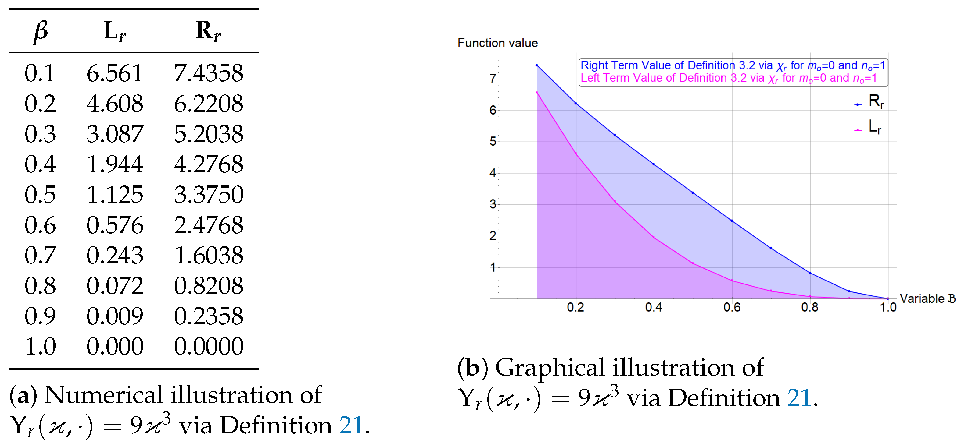
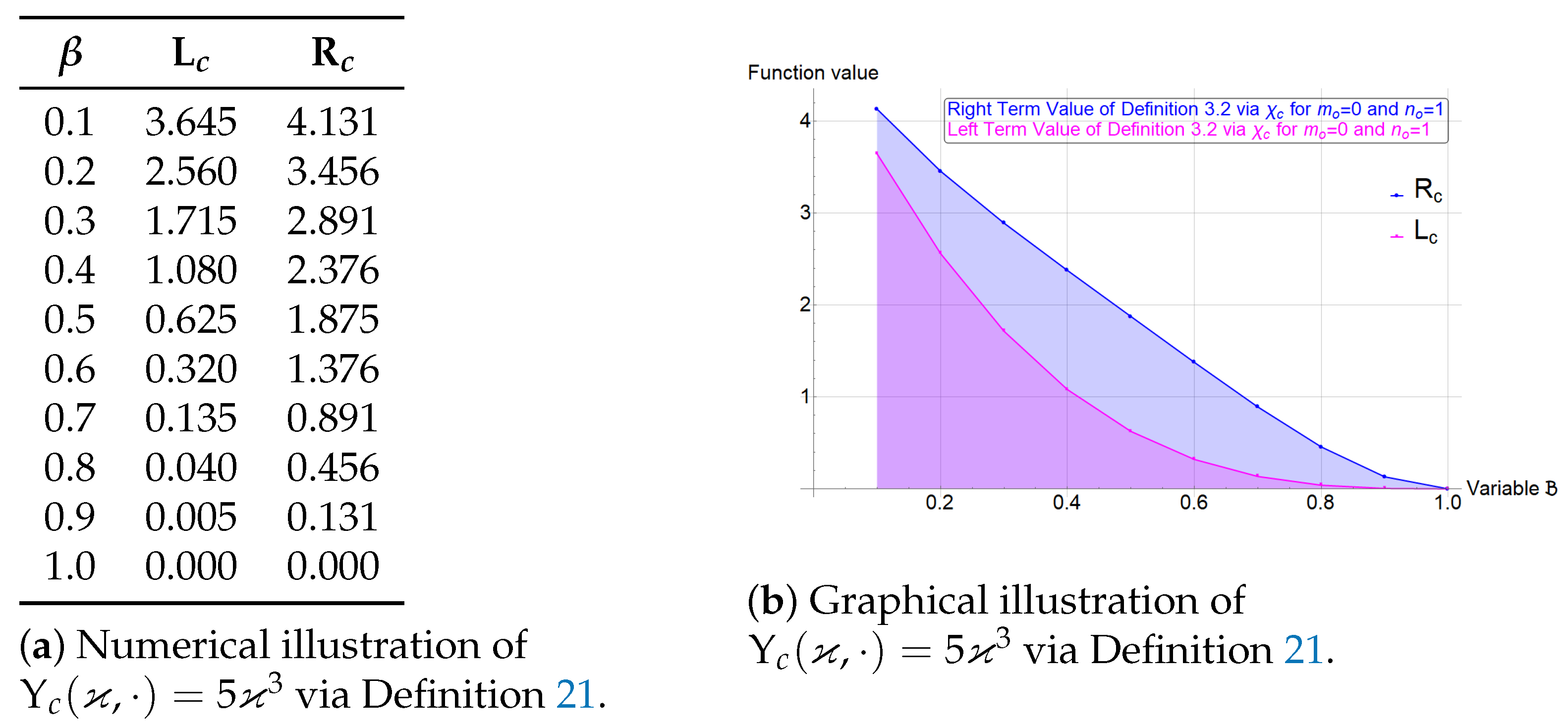
([46]). Let $\Psi :I\subset [0,\infty [⟶\Re$ is assumed to be a superquadratic and integrable on I = $[{\mathfrak{s}}_o,{\mathfrak{t}}_o]$ with $0\le {\mathfrak{s}}_o<{\mathfrak{t}}_o$, then

$$\begin{array}{cc}\hfill & \Psi \left({\displaystyle \frac{{\mathfrak{s}}_o+{\mathfrak{t}}_o}{2}}\right)+{\displaystyle \frac{\beta }{2{({\mathfrak{t}}_o-{\mathfrak{s}}_o)}^{\beta }}}{\int }_{{\mathfrak{s}}_o}^{{\mathfrak{t}}_o}\Psi \left(|{\displaystyle \frac{{\mathfrak{s}}_o+{\mathfrak{t}}_o}{2}}-x|\right)({({\mathfrak{t}}_o-\varkappa )}^{\beta -1}+{(\varkappa -{\mathfrak{s}}_o)}^{\beta -1})d\varkappa \hfill \\ \hfill & \le {\displaystyle \frac{\Gamma (1+\beta )}{2{({\mathfrak{t}}_o-{\mathfrak{s}}_o)}^{\beta }}}\left({\mathfrak{J}}_{{{\mathfrak{s}}_o}^{+}}^{\beta }\Psi \left({\mathfrak{t}}_o\right)+{\mathfrak{J}}_{{{\mathfrak{t}}_o}^{-}}^{\beta }\Psi \left({\mathfrak{s}}_o\right)\right)\hfill \\ \hfill & \le {\displaystyle \frac{\Psi \left({\mathfrak{s}}_o\right)+\Psi \left({\mathfrak{t}}_o\right)}{2}}-{\displaystyle \frac{\beta }{2{({\mathfrak{t}}_o-{\mathfrak{s}}_o)}^{\beta }}}{\int }_{{\mathfrak{s}}_o}^{{\mathfrak{t}}_o}\left(\left({\displaystyle \frac{\varkappa -{\mathfrak{s}}_o}{{\mathfrak{t}}_o-{\mathfrak{s}}_o}}\right)\Psi ({\mathfrak{t}}_o-\varkappa )+\left({\displaystyle \frac{{\mathfrak{t}}_o-\varkappa }{{\mathfrak{t}}_o-{\mathfrak{s}}_o}}\right)\Psi (\varkappa -{\mathfrak{s}}_o)\right)\hfill \\ \hfill & \times ({({\mathfrak{t}}_o-\varkappa )}^{\beta -1}+{(\varkappa -{\mathfrak{s}}_o)}^{\beta -1})d\varkappa ,\hfill \end{array}$$

(5)

where ${\mathfrak{J}}_{{{\mathfrak{s}}_o}^{+}}^{\beta }$, and ${\mathfrak{J}}_{{{\mathfrak{t}}_o}^{-}}^{\beta }$, are defined by Definition 3.

Definition 3. 

Riemann–Liouville fractional integrals of fractional order $\beta \ge 0$, with ${\mathfrak{s}}_o\ge 0$, are stated as

$$\begin{array}{cc}\hfill & {\mathfrak{I}}_{{\mathfrak{s}}_{\mathfrak{o}}}^{\beta }+\Psi \left(\varkappa \right)={\displaystyle \frac{1}{\Gamma \left(\beta \right)}}{\int }_{{\mathfrak{s}}_o}^{\varkappa }{(\varkappa -{\mathrm{y}}_o)}^{\beta -1}\Psi \left({\mathrm{y}}_o\right)d{\mathrm{y}}_o,(\varkappa >{\mathfrak{s}}_o),\hfill \end{array}$$

and

$$\begin{array}{cc}\hfill & {\mathfrak{I}}_{{\mathfrak{t}}_o^{-}}^{\beta }\Psi \left(\varkappa \right)={\displaystyle \frac{1}{\Gamma \left(\beta \right)}}{\int }_{\varkappa }^{{\mathfrak{t}}_o}{({\mathrm{y}}_o-\varkappa )}^{\beta -1}\Psi \left({\mathrm{y}}_o\right)d{\mathrm{y}}_o,(\varkappa <{\mathfrak{t}}_o),\hfill \end{array}$$

the notations ${\mathfrak{I}}_{{\mathfrak{t}}_o^{-}}^{\beta }\Psi \left(\varkappa \right)$ is the right and ${\mathfrak{I}}_{{{\mathfrak{s}}_o}^{+}}^{\beta }\Psi \left(\varkappa \right)$ is the left-sided operators. Where $\Gamma \left(\beta \right)={\int }_0^{\infty }{{\mathrm{y}}_o}^{\beta -1}{e}^{-{\mathrm{y}}_o}d{\mathrm{y}}_o$ is defined as the gamma function.

Now, we derive essential results from interval analysis that are instrumental in establishing the main findings.

Definition 4 

([21]). An interval number $\left[\mathrm{H}\right]$ is the generalization of real number and is defined as

$$\begin{array}{c}\hfill \left[\mathrm{H}\right]=[\underline{\mathrm{H}},\overline{\mathrm{H}}]=\{\varkappa :\underline{\mathrm{H}}\le \varkappa \le \overline{\mathrm{H}},\varkappa \in \Re \},\end{array}$$

$\forall \underline{\mathrm{H}},\overline{\mathrm{H}}\in \Re$ with $\underline{\mathrm{H}}\le \overline{\mathrm{H}}$.

Remark 3. 

Each $\varkappa \in \Re$ can be expressed in an interval form as $[\varkappa ,\varkappa ]$ with zero length.

Let the center of the interval $[\underline{\mathrm{H}},\overline{\mathrm{H}}]$ be represented by ${\mathrm{H}}_c={\displaystyle \frac{\underline{\mathrm{H}}+\overline{\mathrm{H}}}{2}}$ and radius by ${\mathrm{H}}_r={\displaystyle \frac{\overline{\mathrm{H}}-\underline{\mathrm{H}}}{2}}$, then the center-radius form of $[\underline{\mathrm{H}},\overline{\mathrm{H}}]$ is written as

$$\begin{array}{c}\hfill \left[\mathrm{H}\right]=〈{\mathrm{H}}_c,{\mathrm{H}}_r〉=\{\varkappa :{\mathrm{H}}_c-{\mathrm{H}}_r\le \varkappa \le {\mathrm{H}}_c+{\mathrm{H}}_r,\varkappa \in \mathbb{R}\},\end{array}$$

Definition 5 

([53]). The addition, subtraction and multiplication of $\left[\mathrm{H}\right]=〈{\mathrm{H}}_c,{\mathrm{H}}_r〉$ and $\left[\mathrm{v}\right]=〈{\mathrm{v}}_c,{\mathrm{v}}_r〉$ can be defined as follows:

• Addition: $\left[\mathrm{H}\right]+\left[\mathrm{K}\right]=〈{\mathrm{H}}_c,{\mathrm{H}}_r〉+〈{\mathrm{K}}_c,{\mathrm{K}}_r〉=〈{\mathrm{H}}_c+{\mathrm{K}}_c,{\mathrm{H}}_r+{\mathrm{K}}_r〉$.
• Subtraction: $\left[\mathrm{H}\right]-\left[\mathrm{K}\right]=〈{\mathrm{H}}_c,{\mathrm{H}}_r〉-〈{\mathrm{K}}_c,{\mathrm{K}}_r〉=〈{\mathrm{H}}_c,{\mathrm{H}}_r〉+〈-{\mathrm{K}}_c,-{\mathrm{K}}_r〉=〈{\mathrm{H}}_c-{\mathrm{K}}_c,{\mathrm{H}}_r-{\mathrm{K}}_r〉$.
• Multiplication of interval by any real number: For any $\beta \in \mathbb{R}$, we have

  $$\beta \left[\mathrm{H}\right]=\beta 〈{\mathrm{H}}_c,{\mathrm{H}}_r〉=\left\{\begin{array}{cc}〈\beta {\mathrm{H}}_c,\beta {\mathrm{H}}_r〉,& \mathrm{if}\beta \ge 0\\ \\ 〈\beta {\mathrm{H}}_c,-\beta {\mathrm{H}}_r〉,& \mathrm{if}\beta <0.\end{array}\right.$$

or

$$\begin{array}{c}\hfill \beta \left[\mathrm{H}\right]=\beta 〈{\mathrm{H}}_c,{\mathrm{H}}_r〉=〈\beta {\mathrm{H}}_c,\left|\beta \right|{\mathrm{H}}_r〉.\end{array}$$

Definition 6 

([53]). Let $\left[\mathrm{H}\right]=[\underline{\mathrm{H}},\overline{\mathrm{H}}]$ be an interval and $\mathrm{n}\in {\mathbb{Z}}^{+}$ then

$$\begin{array}{c}\hfill {\left[\mathrm{H}\right]}^{\mathrm{n}}=[\underline{{\mathrm{H}}^{\mathrm{n}}},\overline{{\mathrm{H}}^{\mathrm{n}}}],for\underline{\mathrm{H}}\ge 0.\end{array}$$

The centre-radius form of ${\left[\mathrm{H}\right]}^{\mathrm{n}}=[\underline{{\mathrm{H}}^{\mathrm{n}}},\overline{{\mathrm{H}}^{\mathrm{n}}}]$ is written as

$${\left[\mathrm{H}\right]}^{\mathrm{n}}=〈{{\mathrm{H}}_c}^{\mathrm{n}},{{\mathrm{H}}_r}^{\mathrm{n}}〉.$$

where ${{\mathrm{H}}_c}^{\mathfrak{n}}={\displaystyle \frac{{\underline{\mathrm{H}}}^{\mathfrak{n}}+{\overline{\mathrm{H}}}^{\mathfrak{n}}}{2}}$ and ${{\mathrm{H}}_r}^{\mathfrak{n}}={\displaystyle \frac{{\overline{\mathrm{H}}}^{\mathfrak{n}}-{\underline{\mathrm{H}}}^{\mathfrak{n}}}{2}}$.

Definition 7 

([53]). The nth root of $\left[\mathrm{H}\right]=[\underline{\mathrm{H}},\overline{\mathrm{H}}]$ , $\mathrm{n}$ is given by

$$\begin{array}{c}\hfill {\left[\mathrm{H}\right]}^{{\displaystyle \frac{1}{\mathfrak{n}}}}={[\underline{\mathrm{H}},\overline{\mathrm{H}}]}^{{\displaystyle \frac{1}{\mathfrak{n}}}}=\sqrt[n]{[\underline{\mathrm{H}},\overline{\mathrm{H}}]}=[\sqrt[n]{\underline{\mathrm{H}}},\sqrt[n]{\overline{\mathrm{H}}}],for\underline{\mathrm{H}}\ge 0,\end{array}$$

and the centre-radius form of ${\left[\mathrm{H}\right]}^{{\displaystyle \frac{1}{\mathfrak{n}}}}=[\sqrt[n]{\underline{\mathrm{H}}},\sqrt[n]{\overline{\mathrm{H}}}]$ is given by

$$\begin{array}{c}\hfill {\left[\mathrm{H}\right]}^{{\displaystyle \frac{1}{\mathfrak{n}}}}=〈\sqrt[n]{{\mathrm{H}}_c},\sqrt[n]{{\mathrm{H}}_r}〉.\end{array}$$

where $\sqrt[n]{{\mathrm{H}}_c}={\displaystyle \frac{\sqrt[n]{\underline{\mathrm{H}}}+\sqrt[n]{\overline{\mathrm{H}}}}{2}}$ and $\sqrt[n]{{\mathrm{H}}_r}={\displaystyle \frac{\sqrt[n]{\overline{\mathrm{H}}}-\sqrt[n]{\underline{\mathrm{H}}}}{2}}$.

Definition 8 

([53]). The modulus of $\left[\mathrm{H}\right]=[\underline{\mathrm{H}},\overline{\mathrm{H}}]$ is given by

$$\begin{array}{cc}\hfill & \left|\left[\mathrm{H}\right]\right|=|[\underline{\mathrm{H}},\overline{\mathrm{H}}]|=[\underline{\mathrm{H}},\overline{\mathrm{H}}],if\underline{\mathrm{H}}\ge 0\hfill \\ \hfill & =\left[\right|\overline{\mathrm{H}}|,|\underline{\mathrm{H}}\left|\right],if\overline{\mathrm{H}}\le 0\hfill \end{array}$$

and the centre-radius form of $\left|\left[\mathrm{H}\right]\right|=\left|\right[\underline{\mathrm{H}},\overline{\mathrm{H}}\left]\right|$ is given by

$$\begin{array}{cc}\hfill & \left|\left[\mathrm{H}\right]\right|=〈|{\mathrm{H}}_c|,|{\mathrm{H}}_r|〉=〈{\displaystyle \frac{\underline{\mathrm{H}}+\overline{\mathrm{H}}}{2}},{\displaystyle \frac{\overline{\mathrm{H}}-\underline{\mathrm{H}}}{2}}〉,if\underline{\mathrm{H}}\ge 0\hfill \\ \hfill & =〈{\displaystyle \frac{\left|\underline{\mathrm{H}}\right|+\left|\overline{\mathrm{H}}\right|}{2}},{\displaystyle \frac{\left|\underline{\mathrm{H}}\right|-\left|\overline{\mathrm{H}}\right|}{2}}〉,if\overline{\mathrm{H}}\le 0\hfill \end{array}$$

Definition 9 

([27]). Let ${\Re }_I$ be the set of all real closed intervals and for any $\mathrm{H}=[\underline{\mathrm{H}},\overline{\mathrm{H}}]=〈{\mathrm{H}}_c,{\mathrm{H}}_r〉,\mathrm{K}=[\underline{\mathrm{K}},\overline{\mathrm{K}}]=〈{\mathrm{K}}_c,{\mathrm{K}}_r〉\in {\Re }_I$, the center-radius order relation is defined as follows:

$$\mathrm{H}{⪯}_c^r\mathrm{K}\iff \left\{\begin{array}{cc}{\mathrm{H}}_c<{\mathrm{K}}_c,& if{\mathrm{H}}_c\ne {\mathrm{K}}_c\\ \\ {\mathrm{H}}_r\le {\mathrm{K}}_r,& if{\mathrm{H}}_c={\mathrm{K}}_c.\end{array}\right.$$

(6)

Moreover for any $\mathrm{H},\mathrm{K}\in {\Re }_I$, either $\mathrm{H}{⪯}_c^r\mathrm{K}$ or $\mathrm{K}{⪯}_c^r\mathrm{H}$.

The relation ${⪯}_c^r$ holds the following properties, such that for any $\mathrm{H},\mathrm{K},\mathrm{S}\in {\Re }_I$, where $\mathrm{H}=[\underline{\mathrm{H}},\overline{\mathrm{H}}]=〈{\mathrm{H}}_c,{\mathrm{H}}_r〉,\mathrm{K}=[\underline{\mathrm{K}},\overline{\mathrm{K}}]=〈{\mathrm{K}}_c,{\mathrm{K}}_r〉$ and $\mathrm{S}=[\underline{\mathrm{S}},\overline{\mathrm{S}}]=〈{\mathrm{S}}_c,{\mathrm{S}}_r〉$:

• Reflexivity: $\mathrm{H}{⪯}_c^r\mathrm{H}$.
• Anti-symmetry: $\mathrm{H}{⪯}_c^r\mathrm{K}$ and $\mathrm{K}{⪯}_c^r\mathrm{H}$.
• Transitivity: $\mathrm{H}{⪯}_c^r\mathrm{K}$ and $\mathrm{K}{⪯}_c^r\mathrm{S}$ then $\mathrm{H}{⪯}_c^r\mathrm{S}$.
• Comparability: $\mathrm{H}{⪯}_c^r\mathrm{K}$ or $\mathrm{K}{⪯}_c^r\mathrm{H}$.

Theorem 4 

([54]). Let the interval-valued function $\Psi :[{\mathfrak{s}}_o,{\mathfrak{t}}_o]\to {\Re }_I$ given by $\Psi =[\underline{\Psi },\overline{\Psi }]$ is interval Riemann integrable on $[{\mathfrak{s}}_o,{\mathfrak{t}}_o]$ if and only if $\underline{\Psi }$ and $\overline{\Psi }$ are Riemann integrable on $[{\mathfrak{s}}_o,{\mathfrak{t}}_o]$, i.e.,

$$\begin{array}{c}\hfill \left(IR\right){\int }_{{\mathfrak{s}}_o}^{{\mathfrak{t}}_o}\Psi \left(\varkappa \right)d\varkappa =\left[\left(R\right){\int }_{{\mathfrak{s}}_o}^{{\mathfrak{t}}_o}\underline{\Psi }\left(\varkappa \right)d\varkappa ,\left(R\right){\int }_{{\mathfrak{s}}_o}^{{\mathfrak{t}}_o}\overline{\Psi }\left(\varkappa \right)d\varkappa \right].\end{array}$$

(7)

According to the center-radius order relation, the integral preserves the order structure of the intervals.

Theorem 5. 

Let the interval-valued functions $\Psi ,\mathrm{g}:[{\mathfrak{s}}_o$, ${\mathfrak{t}}_o]\to {\Re }_I$ given by $\Psi =[\underline{\Psi },\overline{\Psi }]$ and $\mathrm{g}=[\underline{\mathrm{g}},\overline{\mathrm{g}}]$ and $\Psi \left(\varkappa \right){⪯}_c^r\mathrm{g}\left(\varkappa \right)$, ∀$\varkappa \in [{\mathfrak{s}}_o$, ${\mathfrak{t}}_o]$, then

$$\begin{array}{c}\hfill {\int }_{{\mathfrak{s}}_o}^{{\mathfrak{t}}_o}\Psi \left(\varkappa \right)d\varkappa {⪯}_c^r{\int }_{{\mathfrak{s}}_o}^{{\mathfrak{t}}_o}\mathrm{g}\left(\varkappa \right)d\varkappa .\end{array}$$

(8)

Next, we describe the basic terminologies associated with stochastic analysis:

Definition 10 

([31]). A mapping ${\rm Y}:\Pi \to \Re$ stated on the space $(\Pi ,\mathit{A},\mathrm{P})$ is referred to as a random variable, provided it is $\mathit{A}$-measurable. The space $(\Pi ,\mathrm{A},\mathrm{P})$ is called probability space, in which Π is the set of all possible outcomes, $\mathit{A}$ is a collection of events in other words subsets of Π, while $\mathrm{P}$ is a probability measure that gives these occurrences probabilities.

Example 1. 

Think of a coin toss, where $\Pi =\left\{H\right(Head),T(Tail\left)\right\}$, “$\mathit{A}$” contains whole subsets of Π and “$\mathrm{P}$” gives each possible event a probability of ${\displaystyle \frac{1}{2}}$. Then, a random variable “Υ” would be defined as ${\rm Y}\left(T\right)=1$ and ${\rm Y}\left(H\right)=0.$

Definition 11 

([31]). A mapping ${\rm Y}:I\times \Pi \to \Re$ is referred to as a stochastic process provided ∀ $\varkappa \in I$, ${\rm Y}(\varkappa ,·)$ is a random variable.

Example 2. 

Consider spending a week monitoring the temperature at noon every day. In this case, Π may stand for all potential weather scenarios, $I=\{1,2,\dots ,7\}$, denotes each day of the week, and ${\rm Y}(\varkappa ,\omega )$ provides the temperature on day ϰ under the condition ω. For each fixed day ϰ, ${\rm Y}(\varkappa ,·)$ as a random variable, represents how the temperature changes under various meteorological circumstances. ${\rm Y}(\varkappa ,·)$ represents the stochastic process that describes the temperature over time as ϰ varies.

Definition 12 

([31]). A stochastic process ${\rm Y}:I\times \Pi \to \Re$ is said to possess continuity over $I\subset \Re$, if ∀ $\varkappa \in I$, we have

$$\begin{array}{c}\hfill \mathrm{P}-\underset{\varkappa \to \mathrm{k}}{lim}{\rm Y}(\varkappa ,·)={\rm Y}(\mathrm{k},·),\end{array}$$

where $\mathrm{P}-lim$ displays the limit in the probability space.

Definition 13. 

A stochastic process ${\rm Y}:I\times \Pi \to \Re$ is said to possess mean-square continuity over $I\subset \Re$ if ∀ $\varkappa \in I$, we have

$$\begin{array}{c}\hfill \underset{\varkappa \to \mathrm{k}}{lim}E\left[{({\rm Y}(\varkappa ,·)-{\rm Y}(\mathrm{k},·))}^2\right]=0,\end{array}$$

where $E\left[{\rm Y}(\varkappa ,·)\right]$ represents expectation of the random variable.

Remark 4. 

Mean-square continuity clearly indicates probability continuity, while the opposite conclusion is false.

Definition 14. 

A stochastic process ${\rm Y}:I\times \Pi \to \Re$ is said to possess mean-square differentiability over $I\subset \Re$ at $\mathrm{k}$ if there exists a random variable ${{\rm Y}}^{\prime }:I\times \Pi \to \Re$ such that

$$\begin{array}{c}\hfill {{\rm Y}}^{\prime }(\varkappa ,·)=\mathrm{P}-\underset{\varkappa \to \mathrm{k}}{lim}{\displaystyle \frac{{\rm Y}(\varkappa ,·)-{\rm Y}(\mathrm{k},·)}{\varkappa -\mathrm{k}}},\end{array}$$

Definition 15. 

A stochastic process ${\rm Y}:I\times \Pi \to \Re$, is said to possess mean-square integrability over $I\subset \Re$, if ∀ $\varkappa \in I$, with $E\left[{\rm Y}(\varkappa ,·)\right]<\infty$, $\left[{\varkappa }_1,{\varkappa }_2\right]\subseteq I$, ${\varkappa }_1={\mathfrak{k}}_0<{\mathfrak{k}}_1<{\mathfrak{k}}_2\cdots <{\mathfrak{k}}_n={\varkappa }_2$, partitions the interval $\left[{\varkappa }_1,{\varkappa }_2\right]$, and ${\varkappa }_i\in \left[{\mathfrak{k}}_{i-1},{\mathfrak{k}}_i\right],\forall i=1,\dots ,n$, the subsequent condition holds

$$\begin{array}{c}\hfill \underset{n\to \infty }{lim}E\left[{\left(\sum _{i=1}^n{\rm Y}({\varkappa }_i,·)({\mathfrak{k}}_i-{\mathfrak{k}}_{i-1})-S(·)\right)}^2\right]=0,\end{array}$$

it implies that $S:I\times \Pi \to \Re$, is a mean-square integral of the stochastic process ${\rm Y}:I\times \Pi \to \Re$, and it can be written as

$$\begin{array}{c}\hfill S(·)={\int }_{{\varkappa }_1}^{{\varkappa }_2}{\rm Y}(\varkappa ,·)d\varkappa .\end{array}$$

(9)

Remark 5. 

It is sufficient to presuppose the mean-square continuity of the stochastic process Υ, in order for the mean-square integral to exist.

Remark 6. 

Monotonicity of the mean-square-integral:

This property says that if ${\rm Y}(\varkappa ,·)\le S(\varkappa ,·)$, ∀ $\varkappa \in \left[{\varkappa }_1,{\varkappa }_2\right]$, then

$$\begin{array}{c}\hfill {\int }_{{\varkappa }_1}^{{\varkappa }_2}{\rm Y}(\varkappa ,·)d\varkappa \le {\int }_{{\varkappa }_1}^{{\varkappa }_2}S(\varkappa ,·)d\varkappa .\end{array}$$

(10)

Lemma 3 

([34]). If a stochastic process ${\rm Y}:I\times \Pi \to \Re$ is given by ${\rm Y}(\varkappa ,·)=\mathrm{M}(·)\varkappa +\mathrm{N}(·)$, where $\mathrm{M},\mathrm{N}:\Pi \to \Re$, such that $E\left({\mathrm{M}}^2\right),E\left({\mathrm{N}}^2\right)<\infty$, and $\left[{\varkappa }_1,{\varkappa }_2\right]\subset I$, then

$$\begin{array}{c}\hfill {\int }_{{\varkappa }_1}^{{\varkappa }_2}{\rm Y}(\varkappa ,·)d\varkappa =\mathrm{M}(·){\displaystyle \frac{{{\varkappa }_2}^2-{{\varkappa }_1}^2}{2}}+\mathrm{N}(·)({\varkappa }_2-{\varkappa }_1),\end{array}$$

(11)

where $\mathrm{M}$ and $\mathrm{N}$ are independent, centred random variables with finite second moments.

Definition 16 

([34]). A stochastic process ${\rm Y}:I\times \Pi \to \Re$ is said to be convex over $I\subset \Re$ if

$$\begin{array}{c}\hfill {\rm Y}(\beta {\mathfrak{s}}_o+(1-\beta ){\mathfrak{t}}_o,·)\le \beta {\rm Y}({\mathfrak{s}}_o,·)+(1-\beta ){\rm Y}({\mathfrak{t}}_o,·),\end{array}$$

(12)

holds $\forall \beta \in [0,1]$ and ${\mathfrak{s}}_o,{\mathfrak{t}}_o\in I$.

If $\beta ={\displaystyle \frac{1}{2}}$ is picked in (12), then the process Υ is referred to as Jensen convex. If the process Υ is convex then $(-{\rm Y})$ is then deemed a concave stochastic process. For more intriguing properties, one can see the papers [31,32].

Lemma 4 

([32]). For any ${\varkappa }_1,{\varkappa }_2\in I_o$, such that ${\varkappa }_1<{\varkappa }_2$, then the subsequent inequalities

$$\begin{array}{c}\hfill {{\rm Y}}_{-}^{\prime }({\varkappa }_1,·)\le {{\rm Y}}_{+}^{\prime }({\varkappa }_1,·)\le {{\rm Y}}_{-}^{\prime }({\varkappa }_2,·)\le {{\rm Y}}_{+}^{\prime }({\varkappa }_2,·),\end{array}$$

(13)

where ${{\rm Y}}_{-}^{\prime }$, and ${{\rm Y}}_{+}^{\prime }$, are the left and right derivatives of Υ.

Theorem 6. 

Hermite–Hadamard inequality for convex stochastic process:

If a convex stochastic process ${\rm Y}:I\times \Pi \to \Re$ is possessing mean-square continuity and Jensen’s convexity on I, then the subsequent inequality

$$\begin{array}{c}\hfill {\rm Y}\left({\displaystyle \frac{{\varkappa }_1+{\varkappa }_2}{2}},·\right)\le {\displaystyle \frac{1}{{\varkappa }_2-{\varkappa }_1}}{\int }_{{\varkappa }_1}^{{\varkappa }_2}{\rm Y}(\varkappa ,·)d\varkappa \le {\displaystyle \frac{{\rm Y}({\varkappa }_1,·)+{\rm Y}({\varkappa }_2,·)}{2}},\end{array}$$

(14)

holds ∀  ${\varkappa }_1,{\varkappa }_2\in I$

Definition 17 

([55]). Mean-square stochastic Riemann–Liouville fractional integrals:

Let us have a stochastic process ${\rm Y}:I\times \Pi \to \Re$ fulfilling the conditions given by Definition 15, then mean-square stochastic Riemann–Liouville fractional integrals $I_{{\mathfrak{s}}_o^{+}}^{\alpha }$, and $I_{{\mathfrak{t}}_o^{-}}^{\alpha }$ of Υ, of order $\alpha >0$ are given by

$$\begin{array}{c}\hfill I_{{\mathfrak{s}}_o^{+}}^{\alpha }[{\rm Y}]\left(\varkappa \right)={\displaystyle \frac{1}{\Gamma \left(\alpha \right)}}{\int }_{{\mathfrak{s}}_o}^{\varkappa }{(\varkappa -\mathfrak{s})}^{\alpha -1}{\rm Y}(\mathfrak{s},·)d\mathfrak{s},\varkappa >{\mathfrak{s}}_o,\end{array}$$

and

$$\begin{array}{c}\hfill I_{{\mathfrak{t}}_o^{-}}^{\alpha }[{\rm Y}]\left(\varkappa \right)={\displaystyle \frac{1}{\Gamma \left(\alpha \right)}}{\int }_{\varkappa }^{{\mathfrak{t}}_o}{(\mathfrak{s}-\varkappa )}^{\alpha -1}{\rm Y}(\mathfrak{s},·)d\mathfrak{s},\varkappa <{\mathfrak{t}}_o.\end{array}$$

Now, we present the notion of a center-radius interval-valued stochastic process.

Definition 18 

([56]). Let $\mathfrak{h}:[0,1]\to {\Re }^{+}$, then any interval-valued stochastic process ${\rm Y}(\varkappa ,·)=[\underline{{\rm Y}}(\varkappa ,·),\overline{{\rm Y}}(\varkappa ,·)]$ be a center-radius interval-valued-$\mathfrak{h}$-convex stochastic process, if

$$\begin{array}{cc}\hfill & {\rm Y}(\beta {\mathfrak{s}}_o+(1-\beta ){\mathfrak{t}}_o,·){⪯}_c^r\beta {\rm Y}({\mathfrak{s}}_o,·)+(1-\beta ){\rm Y}({\mathfrak{t}}_o,·),\hfill \end{array}$$

(15)

holds $\forall \beta \in [0,1]$.

The interval-valued stochastic $\mathbb{RL}$ fractional operators are defined as follows.

Definition 19. 

Let ${\rm Y}(\varkappa ,·)=[\underline{{\rm Y}}(\varkappa ,·),\overline{{\rm Y}}(\varkappa ,·)]$, where $\underline{{\rm Y}}(\varkappa ,·)$ and $\overline{{\rm Y}}(\varkappa ,·)$ are the mean square Riemann integrable on $[{\mathfrak{s}}_o,{\mathfrak{t}}_o]$, then

$$\begin{array}{cc}\hfill & {\mathfrak{I}}_{{{\mathfrak{s}}_o}^{+}}^{\beta }{\rm Y}(\varkappa ,·)={\displaystyle \frac{1}{\Gamma \left(\beta \right)}}{\int }_{{\mathfrak{s}}_o}^{\varkappa }{(\varkappa -{\mathrm{y}}_o)}^{\beta -1}{\rm Y}({\mathrm{y}}_o,·)d{\mathrm{y}}_o,(\varkappa >{\mathfrak{s}}_o),\hfill \end{array}$$

and

$$\begin{array}{cc}\hfill & {\mathfrak{I}}_{{\mathfrak{t}}_o^{-}}^{\beta }{\rm Y}(\varkappa ,·)={\displaystyle \frac{1}{\Gamma \left(\beta \right)}}{\int }_{\varkappa }^{{\mathfrak{t}}_o}{({\mathrm{y}}_o-\varkappa )}^{\beta -1}{\rm Y}({\mathrm{y}}_o,·)d{\mathrm{y}}_o,(\varkappa <{\mathfrak{t}}_o),\hfill \end{array}$$

with $\beta \ge 0$. It is to be observed that

$$\begin{array}{c}\hfill {\mathfrak{I}}_{{{\mathfrak{s}}_o}^{+}}^{\beta }{\rm Y}(\varkappa ,·)=[{\mathfrak{I}}_{{{\mathfrak{s}}_o}^{+}}^{\beta }\underline{{\rm Y}}(\varkappa ,·),{\mathfrak{I}}_{{{\mathfrak{s}}_o}^{+}}^{\beta }\overline{{\rm Y}}(\varkappa ,·)],\end{array}$$

(16)

and

$$\begin{array}{c}\hfill {\mathfrak{I}}_{{\mathfrak{t}}_o^{-}}^{\beta }{\rm Y}(\varkappa ,·)=[{\mathfrak{I}}_{{\mathfrak{t}}_o^{-}}^{\beta }\underline{{\rm Y}}(\varkappa ,·),{\mathfrak{I}}_{{\mathfrak{t}}_o^{-}}^{\beta }\overline{{\rm Y}}(\varkappa ,·)]\end{array}$$

(17)

3. Center-Radius Interval-Valued Superquadratic Stochastic Processes and Associated Integral Inequalities

In this section, first of all, we provide a definition for superquadratic stochastic processes, which are generalizations of convex stochastic processes, so that the results developed from superquadratic stochastic processes are more refined as compared to convex stochastic processes. On the basis of this definition, we create the definition of center-radius interval-valued superquadratic stochastic processes and their properties as well as deriving their integral inequalities.

Definition 20. 

A stochastic process ${\rm Y}:I\times \Pi \to \Re$ is said to be superquadratic if

$$\begin{array}{cc}\hfill & {\rm Y}(\beta {\mathfrak{s}}_o+(1-\beta ){\mathfrak{t}}_o,·)\le \beta \left[{\rm Y}({\mathfrak{s}}_o,·)-{\rm Y}((1-\beta )|{\mathfrak{t}}_o-{\mathfrak{s}}_o|,·)\right]\hfill \\ & +(1-\beta )\left[{\rm Y}({\mathfrak{t}}_o,·)-{\rm Y}\left(\beta \right|{\mathfrak{t}}_o-{\mathfrak{s}}_o\left|\right)\right],\hfill \end{array}$$

(18)

holds $\forall {\mathfrak{s}}_o,{\mathfrak{t}}_o\in I$ and $\beta \in [0,1]$.

Remark 7. 

If we choose $\beta ={\displaystyle \frac{1}{2}}$ in (18), then the process Υ is referred to as a Jensen superquadratic.

Remark 8. 

If “≤” is replaced by “≥” then the process Υ is referred to as a subquadratic stochastic process.

Definition 21. 

A mapping ${\rm Y}:I\times \Pi \to {\Re }_I^{+}$ satisfying ${\rm Y}(\varkappa ,·)=[\underline{{\rm Y}}(\varkappa ,·),\overline{{\rm Y}}(\varkappa ,·)]=〈{{\rm Y}}_c(\varkappa ,·),{{\rm Y}}_r(\varkappa ,·)〉$ is said to be center-radius interval-valued superquadratic stochastic process, if

$$\begin{array}{cc}\hfill & {\rm Y}(\beta {\mathfrak{s}}_o+(1-\beta ){\mathfrak{t}}_o,·){⪯}_c^r\beta \left[{\rm Y}({\mathfrak{s}}_o,·)-{\rm Y}((1-\beta )|{\mathfrak{t}}_o-{\mathfrak{s}}_o|,·)\right]\hfill \\ & +(1-\beta )\left[{\rm Y}({\mathfrak{t}}_o,·)-{\rm Y}\left(\beta \right|{\mathfrak{t}}_o-{\mathfrak{s}}_o\left|\right)\right],\hfill \end{array}$$

(19)

holds $\forall \beta \in [0,1]$.

Remark 9. 

If “${⪯}_c^r$” is replaced by “${⪰}_c^r$”, then the process Υ is referred to as a center-radius order interval valued-subquadratic stochastic process.

Remark 10. 

If $\underline{{\rm Y}}(\varkappa ,·)=\overline{{\rm Y}}(\varkappa ,·)$, then we attain Definition 20.

Proposition 1. 

Let ${\rm Y}:I\times \Pi \to {\Re }_I^{+}$ be a center-radius interval-valued superquadratic stochastic process, given by ${\rm Y}(\varkappa ,·)=[\underline{{\rm Y}}(\varkappa ,·),\overline{{\rm Y}}(\varkappa ,·)]=〈{{\rm Y}}_c(\varkappa ,·),{{\rm Y}}_r(\varkappa ,·)〉$ and $\mathrm{k}\in I_o$ (interior of I) and ${\rm Y}(0,·)=0$, then there exists a random variable $\mathrm{A}:\Pi \to {\Re }^{+},$ where $\mathrm{A}\in {\mathrm{L}}^2(\Pi )$ and $\mathrm{A}\left(\omega \right)\ge 0,\forall \omega \in \Pi$ such that ${{\rm Y}}_c$ and ${{\rm Y}}_r$ are supported at $\mathrm{k}$ by the processes $\mathrm{A}(·)(\varkappa -\mathrm{k})+{{\rm Y}}_c(\mathrm{k},·)+{{\rm Y}}_c\left(\right|\varkappa -\mathrm{k}|,·)$ and $\mathrm{A}(·)(\varkappa -\mathrm{k})+{{\rm Y}}_r(\mathrm{k},·)+{{\rm Y}}_r\left(\right|\varkappa -\mathrm{k}|,·)$, respectively, then $\forall \varkappa \in I$

$$\begin{array}{c}\hfill \mathrm{A}(·)(\varkappa -\mathrm{k})+{\rm Y}(\mathrm{k},·)+{\rm Y}\left(\right|\varkappa -\mathrm{k}|,·){⪯}_c^r{\rm Y}(\varkappa ,·).\end{array}$$

(20)

Proof. 

We choose $\mathfrak{r},\mathfrak{s},\mathfrak{u},\mathfrak{v},\mathrm{k}\in I_o$, so that $\mathfrak{r}<\mathfrak{s}<\mathrm{k}<\mathfrak{u}<\mathfrak{v}$. First, considering $\mathfrak{r}<\mathfrak{s}<\mathrm{k}$, we have,

$$\begin{array}{c}\hfill \mathfrak{s}={\displaystyle \frac{\mathrm{k}-\mathfrak{s}}{\mathrm{k}-\mathfrak{r}}}\mathfrak{r}+{\displaystyle \frac{\mathfrak{s}-\mathfrak{r}}{\mathrm{k}-\mathfrak{r}}}\mathrm{k},\end{array}$$

(21)

which is a convex combination of $\mathrm{k}$ and $\mathfrak{r}$. We know that Υ is a center-radius interval-valued superquadratic stochastic process; therefore, ${{\rm Y}}_c$ and ${{\rm Y}}_r$ are superquadratic stochastic processes

$$\begin{array}{c}\hfill {{\rm Y}}_c(\mathfrak{s},·)=\left({\displaystyle \frac{\mathrm{k}-\mathfrak{s}}{\mathrm{k}-\mathfrak{r}}}\right)\left[{{\rm Y}}_c(\mathfrak{r},·)-{{\rm Y}}_c\left(\right|\mathfrak{s}-\mathfrak{r}|,·)\right]+\left({\displaystyle \frac{\mathfrak{s}-\mathfrak{r}}{\mathrm{k}-\mathfrak{r}}}\right)\left[{{\rm Y}}_c(\mathrm{k},·)-{{\rm Y}}_c\left(\right|\mathrm{k}-\mathfrak{s}|,·)\right],\end{array}$$

(22)

after a simple calculation, we achieve the following expression

$$\begin{array}{cc}\hfill & {\displaystyle \frac{{{\rm Y}}_c(\mathrm{k},·)-{{\rm Y}}_c(\mathfrak{r},·)}{\mathrm{k}-\mathfrak{r}}}\le {\displaystyle \frac{{{\rm Y}}_c(\mathrm{k},·)-{{\rm Y}}_c(\mathfrak{s},·)}{\mathrm{k}-\mathfrak{s}}}-{\displaystyle \frac{{{\rm Y}}_c\left(\right|\mathfrak{s}-\mathfrak{r}|,·)-{{\rm Y}}_c\left(\right|\mathrm{k}-\mathfrak{s}|,·)}{\mathrm{k}-\mathfrak{r}}}-{\displaystyle \frac{{{\rm Y}}_c\left(\right|\mathrm{k}-\mathfrak{s}|,·)}{\mathrm{k}-\mathfrak{s}}},\hfill \end{array}$$

(23)

taking limit $\mathfrak{s}\to {\mathrm{k}}^{-}$, on both sides of (23), we get

$$\begin{array}{cc}\hfill & {\displaystyle \frac{{{\rm Y}}_c(\mathrm{k},·)-{{\rm Y}}_c(\mathfrak{r},·)+{{\rm Y}}_c\left(\right|\mathrm{k}-\mathfrak{r}|,·)}{\mathrm{k}-\mathfrak{r}}}\le {{{\rm Y}}_c^{\prime }}_{-}(\mathrm{k},·).\hfill \end{array}$$

(24)

Similarly for $\mathrm{k}<\mathfrak{u}<\mathfrak{v}$, we have

$$\begin{array}{cc}\hfill & {\displaystyle \frac{{{\rm Y}}_c(\mathfrak{u},·)-{{\rm Y}}_c(\mathrm{k},·)}{\mathfrak{u}-\mathrm{k}}}\le {\displaystyle \frac{{{\rm Y}}_c(\mathfrak{v},·)-{{\rm Y}}_c(\mathrm{k},·)}{\mathfrak{v}-\mathrm{k}}}+{\displaystyle \frac{{{\rm Y}}_c\left(\right|\mathfrak{u}-\mathrm{k}|,·)-{{\rm Y}}_c\left(\right|\mathfrak{v}-\mathfrak{u}|,·)}{\mathfrak{v}-\mathrm{k}}}-{\displaystyle \frac{{{\rm Y}}_c\left(\right|\mathfrak{u}-\mathrm{k}|,·)}{\mathfrak{u}-\mathrm{k}}},\hfill \end{array}$$

(25)

taking limit $\mathfrak{u}\to {\mathrm{k}}^{+}$, on both sides of (25), we arrive at

$$\begin{array}{cc}\hfill & {{{\rm Y}}_c^{\prime }}_{+}(\mathrm{k},·)\le {\displaystyle \frac{{{\rm Y}}_c(\mathfrak{v},·)-{{\rm Y}}_c(\mathrm{k},·)-{{\rm Y}}_c\left(\right|\mathfrak{v}-\mathrm{k}|,·)}{\mathfrak{v}-\mathrm{k}}}.\hfill \end{array}$$

(26)

From inequalities (24), (26) and utilization of Lemma 4, implies that

$$\begin{array}{cc}\hfill & {\displaystyle \frac{{{\rm Y}}_c(\mathrm{k},·)-{{\rm Y}}_c(\mathfrak{r},·)+{{\rm Y}}_c\left(\right|\mathrm{k}-\mathfrak{r}|,·)}{\mathrm{k}-\mathfrak{r}}}\le {{{\rm Y}}_c^{\prime }}_{-}(\mathrm{k},·)\le {{{\rm Y}}_c^{\prime }}_{+}(\mathrm{k},·)\hfill \\ & \le {\displaystyle \frac{{{\rm Y}}_c(\mathfrak{v},·)-{{\rm Y}}_c(\mathrm{k},·)-{{\rm Y}}_c\left(\right|\mathfrak{v}-\mathrm{k}|,·)}{\mathfrak{v}-\mathrm{k}}}.\hfill \end{array}$$

(27)

Now, if $\mathrm{A}:\Pi \to {\Re }^{+}$, is any random variable fulfilling the condition ${{{\rm Y}}_c^{\prime }}_{-}(\mathrm{k},·)\le \mathrm{A}(·)\le {{{\rm Y}}_c^{\prime }}_{+}(\mathrm{k},·)$, and setting it into (27) as well as setting $\mathfrak{v}=\varkappa$, we obtain

$$\begin{array}{c}\hfill {{\rm Y}}_c(\varkappa ,·)\ge \mathrm{A}(·)(\varkappa -\mathrm{k})+{{\rm Y}}_c(\mathrm{k},·)+{{\rm Y}}_c\left(\right|\varkappa -\mathrm{k}|,·).\end{array}$$

(28)

Moving in the same fashion as for ${{\rm Y}}_c$ we have the following result for ${{\rm Y}}_r$

$$\begin{array}{c}\hfill {{\rm Y}}_r(\varkappa ,·)\ge \mathrm{A}(·)(\varkappa -\mathrm{k})+{{\rm Y}}_r(\mathrm{k},·)+{{\rm Y}}_r\left(\right|\varkappa -\mathrm{k}|,·).\end{array}$$

(29)

The results (28) and (29) represent the RHS (right-hand side) of the Definition 9; therefore, these can be expressed in the interval form as

$$\begin{array}{cc}\hfill & 〈\mathrm{A}(·)(\varkappa -\mathrm{k})+{{\rm Y}}_c(\mathrm{k},·)+{{\rm Y}}_c\left(\right|\varkappa -\mathrm{k}|,·),\mathrm{A}(·)(\varkappa -\mathrm{k})+{{\rm Y}}_r(\mathrm{k},·)+{{\rm Y}}_r\left(\right|\varkappa -\mathrm{k}|,·)〉\hfill \\ & {⪯}_c^r〈{{\rm Y}}_c(\varkappa ,·),{{\rm Y}}_r(\varkappa ,·)〉.\hfill \end{array}$$

(30)

It implies that

$$\begin{array}{c}\hfill \mathrm{A}(·)(\varkappa -\mathrm{k})+{\rm Y}(\mathrm{k},·)+{\rm Y}\left(\right|\varkappa -\mathrm{k}|,·){⪯}_c^r{\rm Y}(\varkappa ,·).\end{array}$$

(31)

Hence the proof. □

Remark 11. 

If $\underline{{\rm Y}}(\varkappa ,·)=\overline{{\rm Y}}(\varkappa ,·)$, then we attain the result for the superquadratic stochastic process.

Consider the following examples, which consist of tabular and graphical illustrations, and verify the authenticity of Definition 21.

Example 3. 

Let the process ${\rm Y}:I\times \Pi \to {\Re }_I^{+}$ given by ${\rm Y}(\varkappa ,·)=[-4{\varkappa }^3,14{\varkappa }^3]$ on [0, 1] is a $\mathbb{IV}$-stochastic process. The process ${\rm Y}(\varkappa ,·)$ is centre-radius interval-valued superquadratic stochastic if it satisfies Definition 21. Here, ${{\rm Y}}_c(\varkappa ,·)=5{\varkappa }^3$ and ${{\rm Y}}_r(\varkappa ,·)=9{\varkappa }^3$. The graph and table given by Figure 1, confirm that ${{\rm Y}}_r(\varkappa ,·)$ satisfies the condition of Definition 21, while the graph and table given in Figure 2 confirm that ${{\rm Y}}_c(\varkappa ,·)$ satisfies the condition of Definition 21. Let $L_r$ and $R_r$ represent the left and right terms of the condition of Definition 21 for ${{\rm Y}}_r(\varkappa ,·)$ and $L_c$ and $R_c$ represent the left and right terms of the condition of Definition 21 for ${{\rm Y}}_c(\varkappa ,·)$.

Next, we provide the proof of a Jensen’s-type inequality for a center-radius interval-valued superquadratic stochastic process.

Theorem 7. 

Let ${\rm Y}:I\times \Pi \to {\Re }_I^{+}$ be a center-radius interval-valued superquadratic stochastic process, given by ${\rm Y}(\varkappa ,·)=[\underline{{\rm Y}}(\varkappa ,·),\overline{{\rm Y}}(\varkappa ,·)]=〈{{\rm Y}}_c(\varkappa ,·),{{\rm Y}}_r(\varkappa ,·)〉$, then $\forall {\varkappa }_1,\dots ,{\varkappa }_n\in I,{\beta }_1,\dots ,{\beta }_{\mathfrak{n}}>0$, such that ${\sum }_{i=1}^{\mathfrak{n}}{\beta }_i=1$ and $\widehat{\varkappa }={\sum }_{i=1}^{\mathfrak{n}}{\beta }_i{\varkappa }_i$ the inequality

$$\begin{array}{cc}\hfill & {\rm Y}(\widehat{\varkappa },·)+\sum _{i=1}^{\mathfrak{n}}{\beta }_i{\rm Y}\left(\right|{\varkappa }_i-\widehat{\varkappa }|,·){⪯}_c^r\sum _{i=1}^{\mathfrak{n}}{\beta }_i{\rm Y}({\varkappa }_i,·),\hfill \end{array}$$

(32)

holds.

Proof. 

Let ${\varkappa }_i\in I,{\beta }_i>0$, such that ${\sum }_{i=1}^{\mathfrak{n}}{\beta }_i=1$ and $\widehat{\varkappa }={\sum }_{i=1}^{\mathfrak{n}}{\beta }_i{\varkappa }_i$. Since this is a center-radius order interval valued-superquadratic stochastic process, ${{\rm Y}}_c$ and ${{\rm Y}}_r$ are superquadratic stochastic processes. According to Proposition 1, we have a support

$$\begin{array}{c}\hfill \mathrm{A}(·)(\varkappa -\widehat{\varkappa })+{\rm Y}(\widehat{\varkappa },·)+{\rm Y}\left(\right|\varkappa -\widehat{\varkappa }|,·){⪯}_c^r{\rm Y}(\varkappa ,·),\end{array}$$

(33)

at $\widehat{\varkappa }$. Then, for every $i\in \{1,\dots ,n\}$, we have

$$\begin{array}{c}\hfill \mathrm{A}(·)({\varkappa }_i-\widehat{\varkappa })+{\rm Y}(\widehat{\varkappa },·)+{\rm Y}\left(\right|{\varkappa }_i-\widehat{\varkappa }|,·){⪯}_c^r{\rm Y}({\varkappa }_i,·),\end{array}$$

(34)

multiplying the inequality (34) by ${\beta }_i$ and then summing up to $\mathrm{n}$, we obtain

$$\begin{array}{c}\hfill \mathrm{A}(·)\sum _{i=1}^n{\beta }_i({\varkappa }_i-\widehat{\varkappa })+\sum _{i=1}^n{\beta }_i{\rm Y}(\widehat{\varkappa },·)+\sum _{i=1}^n{\beta }_i{\rm Y}\left(\right|{\varkappa }_i-\widehat{\varkappa }|,·){⪯}_c^r\sum _{i=1}^n{\beta }_i{\rm Y}({\varkappa }_i,·),\end{array}$$

(35)

as we know that ${\sum }_{i=1}^n{\beta }_i({\varkappa }_i-\widehat{\varkappa })=0$ and ${\sum }_{i=1}^n{\beta }_i{\rm Y}(\widehat{\varkappa },·)={\rm Y}(\widehat{\varkappa },·){\sum }_{i=1}^n{\beta }_i={\rm Y}(\widehat{\varkappa },·)$ therefore (35) becomes

$$\begin{array}{c}\hfill {\rm Y}(\widehat{\varkappa },·)+\sum _{i=1}^n{\beta }_i{\rm Y}\left(\right|{\varkappa }_i-\widehat{\varkappa }|,·){⪯}_c^r\sum _{i=1}^n{\beta }_i{\rm Y}({\varkappa }_i,·).\end{array}$$

(36)

Hence the proof. □

Remark 12. 

If $\underline{{\rm Y}}(\varkappa ,·)=\overline{{\rm Y}}(\varkappa ,·)$, then we attain the inequality of Jensen’s type for superquadratic stochastic process.

Next, we offer the Hermite–Hadamard inequality for a center-radius interval-valued superquadratic stochastic process.

Theorem 8. 

Let ${\rm Y}:I\times \Pi \to {\Re }_I^{+}$ be a center-radius order interval valued-superquadratic stochastic process, given by ${\rm Y}(\varkappa ,·)=[\underline{{\rm Y}}(\varkappa ,·),\overline{{\rm Y}}(\varkappa ,·)]=〈{{\rm Y}}_c(\varkappa ,·),{{\rm Y}}_r(\varkappa ,·)〉$ and each ${{\rm Y}}_c(\varkappa ,·)$ and ${{\rm Y}}_r(\varkappa ,·)$ possess Jensen superquadraticity and mean-square continuity on I, then

$$\begin{array}{cc}\hfill & {\rm Y}\left({\displaystyle \frac{{\mathfrak{s}}_o+{\mathfrak{t}}_o}{2}},·\right)+{\displaystyle \frac{1}{{\mathfrak{t}}_o-{\mathfrak{s}}_o}}{\int }_{{\mathfrak{s}}_o}^{{\mathfrak{t}}_o}{\rm Y}\left(|\varkappa -{\displaystyle \frac{{\mathfrak{s}}_o+{\mathfrak{t}}_o}{2}}|,·\right)d\varkappa {⪯}_c^r{\displaystyle \frac{1}{{\mathfrak{t}}_o-{\mathfrak{s}}_o}}{\int }_{{\mathfrak{s}}_o}^{{\mathfrak{t}}_o}{\rm Y}(\varkappa ,·)d\varkappa \hfill \\ \hfill & {⪯}_c^r{\displaystyle \frac{{\rm Y}({\mathfrak{s}}_o,·)+{\rm Y}({\mathfrak{t}}_o,·)}{2}}-{\displaystyle \frac{1}{{({\mathfrak{t}}_o-{\mathfrak{s}}_o)}^2}}{\int }_{{\mathfrak{s}}_o}^{{\mathfrak{t}}_o}[({\mathfrak{t}}_o-\varkappa ){\rm Y}(\varkappa -{\mathfrak{s}}_o,·)+(\varkappa -{\mathfrak{s}}_o){\rm Y}({\mathfrak{t}}_o-\varkappa ,·)]d\varkappa ,\hfill \end{array}$$

(37)

holds ∀ ${\mathfrak{s}}_o,{\mathfrak{t}}_o\in I$

Proof. 

Since ${\rm Y}(\varkappa ,·)=〈{{\rm Y}}_c(\varkappa ,·),{{\rm Y}}_r(\varkappa ,·)〉$ is a center-radius interval-valued superquadratic stochastic process, ${{\rm Y}}_c(\varkappa ,·)$ and ${{\rm Y}}_r(\varkappa ,·)$ are mean-square continuous superquadratic stochastic processes; therefore, ${\rm Y}(\varkappa ,·)$ is a mean-square continuous superquadratic stochastic process. By Proposition 1, ${\rm Y}(\varkappa ,·)$ has a supporting process, ∀$\mathrm{k}\in I_o$. Let’s pick $\mathrm{k}={\displaystyle \frac{{\mathfrak{s}}_o+{\mathfrak{t}}_o}{2}}$ in a support, we have

$$\begin{array}{c}\hfill \mathrm{A}(·)\left(\varkappa -{\displaystyle \frac{{\mathfrak{s}}_o+{\mathfrak{t}}_o}{2}}\right)+{\rm Y}\left({\displaystyle \frac{{\mathfrak{s}}_o+{\mathfrak{t}}_o}{2}},·\right)+{\rm Y}\left(|\varkappa -{\displaystyle \frac{{\mathfrak{s}}_o+{\mathfrak{t}}_o}{2}}|,·\right){⪯}_c^r{\rm Y}(\varkappa ,·).\end{array}$$

(38)

The result (38) in the center-radius interval form can be written as

$$\begin{array}{cc}\hfill & \langle \mathrm{A}(·)\left(\varkappa -{\displaystyle \frac{{\mathfrak{s}}_o+{\mathfrak{t}}_o}{2}}\right)+{{\rm Y}}_c\left({\displaystyle \frac{{\mathfrak{s}}_o+{\mathfrak{t}}_o}{2}},·\right)+{{\rm Y}}_c\left(\left|\varkappa -{\displaystyle \frac{{\mathfrak{s}}_o+{\mathfrak{t}}_o}{2}}\right|,·\right)\hfill \\ & ,\mathrm{A}(·)\left(\varkappa -{\displaystyle \frac{{\mathfrak{s}}_o+{\mathfrak{t}}_o}{2}}\right)+{{\rm Y}}_r\left({\displaystyle \frac{{\mathfrak{s}}_o+{\mathfrak{t}}_o}{2}},·\right)+{{\rm Y}}_r\left(\left|\varkappa -{\displaystyle \frac{{\mathfrak{s}}_o+{\mathfrak{t}}_o}{2}}\right|,·\right)\rangle \hfill \\ \hfill & {⪯}_c^r〈{{\rm Y}}_c(\varkappa ,·),{{\rm Y}}_r(\varkappa ,·)〉.\hfill \end{array}$$

(39)

from Definition 9, the result (39) is written as

$$\begin{array}{c}\hfill \mathrm{A}(·)\left(\varkappa -{\displaystyle \frac{{\mathfrak{s}}_o+{\mathfrak{t}}_o}{2}}\right)+{{\rm Y}}_c\left({\displaystyle \frac{{\mathfrak{s}}_o+{\mathfrak{t}}_o}{2}},·\right)+{{\rm Y}}_c\left(|\varkappa -{\displaystyle \frac{{\mathfrak{s}}_o+{\mathfrak{t}}_o}{2}}|,·\right)\le {{\rm Y}}_c(\varkappa ,·),\end{array}$$

(40)

and

$$\begin{array}{c}\hfill \mathrm{A}(·)\left(\varkappa -{\displaystyle \frac{{\mathfrak{s}}_o+{\mathfrak{t}}_o}{2}}\right)+{{\rm Y}}_r\left({\displaystyle \frac{{\mathfrak{s}}_o+{\mathfrak{t}}_o}{2}},·\right)+{{\rm Y}}_r\left(|\varkappa -{\displaystyle \frac{{\mathfrak{s}}_o+{\mathfrak{t}}_o}{2}}|,·\right)\le {{\rm Y}}_r(\varkappa ,·).\end{array}$$

(41)

First considering (40) and integrating it over $[{\mathfrak{s}}_o,{\mathfrak{t}}_o]$. Then, using Lemma 3, we attain

$$\begin{array}{cc}\hfill & {\int }_{{\mathfrak{s}}_o}^{{\mathfrak{t}}_o}{{\rm Y}}_c(\varkappa ,·)d\varkappa \ge {\int }_{{\mathfrak{s}}_o}^{{\mathfrak{t}}_o}\left[\mathrm{A}(·)\left(\varkappa -{\displaystyle \frac{{\mathfrak{s}}_o+{\mathfrak{t}}_o}{2}}\right)+{{\rm Y}}_c\left({\displaystyle \frac{{\mathfrak{s}}_o+{\mathfrak{t}}_o}{2}},·\right)\right]d\varkappa \hfill \\ & +{\int }_{{\mathfrak{s}}_o}^{{\mathfrak{t}}_o}{{\rm Y}}_c\left(|\varkappa -{\displaystyle \frac{{\mathfrak{s}}_o+{\mathfrak{t}}_o}{2}}|,·\right)d\varkappa ={\displaystyle \frac{\mathrm{A}(·)}{2}}({\mathfrak{t}}_o^2-{\mathfrak{s}}_o^2)-{\displaystyle \frac{\mathrm{A}(·)}{2}}({\mathfrak{t}}_o^2-{\mathfrak{s}}_o^2)\hfill \\ & +{{\rm Y}}_c\left({\displaystyle \frac{{\mathfrak{s}}_o+{\mathfrak{t}}_o}{2}},·\right)({\mathfrak{t}}_o-{\mathfrak{s}}_o)+{\int }_{{\mathfrak{s}}_o}^{{\mathfrak{t}}_o}{{\rm Y}}_c\left(|\varkappa -{\displaystyle \frac{{\mathfrak{s}}_o+{\mathfrak{t}}_o}{2}}|,·\right)d\varkappa \hfill \\ & ={{\rm Y}}_c\left({\displaystyle \frac{{\mathfrak{s}}_o+{\mathfrak{t}}_o}{2}},·\right)({\mathfrak{t}}_o-{\mathfrak{s}}_o)+{\int }_{{\mathfrak{s}}_o}^{{\mathfrak{t}}_o}{{\rm Y}}_c\left(|\varkappa -{\displaystyle \frac{{\mathfrak{s}}_o+{\mathfrak{t}}_o}{2}}|,·\right)d\varkappa .\hfill \end{array}$$

(42)

Similarly, considering (41), we have

$$\begin{array}{cc}\hfill & {\int }_{{\mathfrak{s}}_o}^{{\mathfrak{t}}_o}{{\rm Y}}_r(\varkappa ,·)d\varkappa \ge {{\rm Y}}_r\left({\displaystyle \frac{{\mathfrak{s}}_o+{\mathfrak{t}}_o}{2}},·\right)({\mathfrak{t}}_o-{\mathfrak{s}}_o)+{\int }_{{\mathfrak{s}}_o}^{{\mathfrak{t}}_o}{{\rm Y}}_r\left(\left|\varkappa -{\displaystyle \frac{{\mathfrak{s}}_o+{\mathfrak{t}}_o}{2}}\right|,·\right)d\varkappa .\hfill \end{array}$$

(43)

Inequalities (42) and (43) represent the RHS of Definition 9; therefore, we have

$$\begin{array}{cc}\hfill & \langle {{\rm Y}}_c\left({\displaystyle \frac{{\mathfrak{s}}_o+{\mathfrak{t}}_o}{2}},·\right)({\mathfrak{t}}_o-{\mathfrak{s}}_o)+{\int }_{{\mathfrak{s}}_o}^{{\mathfrak{t}}_o}{{\rm Y}}_c\left(\left|\varkappa -{\displaystyle \frac{{\mathfrak{s}}_o+{\mathfrak{t}}_o}{2}}\right|,·\right)d\varkappa \hfill \\ & ,{{\rm Y}}_r\left({\displaystyle \frac{{\mathfrak{s}}_o+{\mathfrak{t}}_o}{2}},·\right)({\mathfrak{t}}_o-{\mathfrak{s}}_o)+{\int }_{{\mathfrak{s}}_o}^{{\mathfrak{t}}_o}{{\rm Y}}_r\left(|\varkappa -{\displaystyle \frac{{\mathfrak{s}}_o+{\mathfrak{t}}_o}{2}}|,·\right)d\varkappa \rangle \hfill \\ & {⪯}_c^r〈{\int }_{{\mathfrak{s}}_o}^{{\mathfrak{t}}_o}{{\rm Y}}_c(\varkappa ,·)d\varkappa ,{\int }_{{\mathfrak{s}}_o}^{{\mathfrak{t}}_o}{{\rm Y}}_r(\varkappa ,·)d\varkappa 〉.\hfill \end{array}$$

(44)

This implies that

$$\begin{array}{cc}\hfill & {\rm Y}\left({\displaystyle \frac{{\mathfrak{s}}_o+{\mathfrak{t}}_o}{2}},·\right)({\mathfrak{t}}_o-{\mathfrak{s}}_o)+{\int }_{{\mathfrak{s}}_o}^{{\mathfrak{t}}_o}{\rm Y}\left(\left|\varkappa -{\displaystyle \frac{{\mathfrak{s}}_o+{\mathfrak{t}}_o}{2}}\right|,·\right)d\varkappa {⪯}_c^r{\int }_{{\mathfrak{s}}_o}^{{\mathfrak{t}}_o}{\rm Y}(\varkappa ,·)d\varkappa .\hfill \end{array}$$

(45)

Again, utilizing the Definition 20 for ${{\rm Y}}_c(\varkappa ,·)$ and setting $\beta {\mathfrak{s}}_o+(1-\beta ){\mathfrak{t}}_o=\varkappa$, in (18), we get

$$\begin{array}{cc}\hfill & {{\rm Y}}_c(\varkappa ,·)\le \left({\displaystyle \frac{{\mathfrak{t}}_o-\varkappa }{{\mathfrak{t}}_o-{\mathfrak{s}}_o}}\right)\left[{{\rm Y}}_c({\mathfrak{s}}_o,·)-{{\rm Y}}_c(\varkappa -{\mathfrak{s}}_o,·)\right]+\left(1-{\displaystyle \frac{{\mathfrak{t}}_o-\varkappa }{{\mathfrak{t}}_o-{\mathfrak{s}}_o}}\right)\left[{{\rm Y}}_c({\mathfrak{t}}_o,·)-{{\rm Y}}_c({\mathfrak{t}}_o-\varkappa ,·)\right]\hfill \\ \hfill & ={\displaystyle \frac{{{\rm Y}}_c({\mathfrak{t}}_o,·)-{{\rm Y}}_c({\mathfrak{s}}_o,·)}{{\mathfrak{t}}_o-{\mathfrak{s}}_o}}\varkappa +{\displaystyle \frac{{\mathfrak{s}}_o{{\rm Y}}_c({\mathfrak{t}}_o,·)-{\mathfrak{t}}_o{{\rm Y}}_c({\mathfrak{s}}_o,·)}{{\mathfrak{t}}_o-{\mathfrak{s}}_o}}\hfill \\ \hfill & -{\displaystyle \frac{1}{{\mathfrak{t}}_o-{\mathfrak{s}}_o}}\left[({\mathfrak{t}}_o-\varkappa ){{\rm Y}}_c(\varkappa -{\mathfrak{s}}_o,·)+(\varkappa -{\mathfrak{s}}_o){{\rm Y}}_c({\mathfrak{t}}_o-\varkappa ,·)\right].\hfill \end{array}$$

(46)

Integrating over $[{\mathfrak{s}}_o,{\mathfrak{t}}_o]$, and again using Lemma 3, we attain

$$\begin{array}{cc}\hfill & {\int }_{{\mathfrak{s}}_o}^{{\mathfrak{t}}_o}{{\rm Y}}_c(\varkappa ,·)d\varkappa \le {\displaystyle \frac{{{\rm Y}}_c({\mathfrak{t}}_o,·)-{{\rm Y}}_c({\mathfrak{s}}_o,·)}{{\mathfrak{t}}_o-{\mathfrak{s}}_o}}{\displaystyle \frac{{\mathfrak{t}}_o^2-{\mathfrak{s}}_o^2}{2}}+{\displaystyle \frac{{\mathfrak{s}}_o{{\rm Y}}_c({\mathfrak{t}}_o,·)-{\mathfrak{t}}_o{{\rm Y}}_c({\mathfrak{s}}_o,·)}{{\mathfrak{t}}_o-{\mathfrak{s}}_o}}({\mathfrak{t}}_o-{\mathfrak{s}}_o)\hfill \\ \hfill & -{\displaystyle \frac{1}{{\mathfrak{t}}_o-{\mathfrak{s}}_o}}{\int }_{{\mathfrak{s}}_o}^{{\mathfrak{t}}_o}\left[({\mathfrak{t}}_o-\varkappa ){{\rm Y}}_c(\varkappa -{\mathfrak{s}}_o,·)+(\varkappa -{\mathfrak{s}}_o){{\rm Y}}_c({\mathfrak{t}}_o-\varkappa ,·)\right]d\varkappa \hfill \\ \hfill & ={\displaystyle \frac{{{\rm Y}}_c({\mathfrak{t}}_o,·)({\mathfrak{s}}_o+{\mathfrak{t}}_o-2{\mathfrak{s}}_o)+{{\rm Y}}_c({\mathfrak{s}}_o,·)(-({\mathfrak{s}}_o+{\mathfrak{t}}_o)+2{\mathfrak{t}}_o)}{2}}\hfill \\ \hfill & -{\displaystyle \frac{1}{{\mathfrak{t}}_o-{\mathfrak{s}}_o}}{\int }_{{\mathfrak{s}}_o}^{{\mathfrak{t}}_o}\left[({\mathfrak{t}}_o-\varkappa ){{\rm Y}}_c(\varkappa -{\mathfrak{s}}_o,·)+(\varkappa -{\mathfrak{s}}_o){{\rm Y}}_c({\mathfrak{t}}_o-\varkappa ,·)\right]d\varkappa .\hfill \end{array}$$

(47)

This implies that

$$\begin{array}{cc}\hfill & {\displaystyle \frac{1}{{\mathfrak{t}}_o-{\mathfrak{s}}_o}}{\int }_{{\mathfrak{s}}_o}^{{\mathfrak{t}}_o}{{\rm Y}}_c(\varkappa ,·)d\varkappa \le {\displaystyle \frac{{{\rm Y}}_c({\mathfrak{t}}_o,·)+{{\rm Y}}_c({\mathfrak{s}}_o,·)}{2}}\hfill \\ \hfill & -{\displaystyle \frac{1}{{({\mathfrak{t}}_o-{\mathfrak{s}}_o)}^2}}{\int }_{{\mathfrak{s}}_o}^{{\mathfrak{t}}_o}\left[({\mathfrak{t}}_o-\varkappa ){{\rm Y}}_c(\varkappa -{\mathfrak{s}}_o,·)+(\varkappa -{\mathfrak{s}}_o){{\rm Y}}_c({\mathfrak{t}}_o-\varkappa ,·)\right]d\varkappa .\hfill \end{array}$$

(48)

Similarly, for ${{\rm Y}}_r(\varkappa ,·)$ we have

$$\begin{array}{cc}\hfill & {\displaystyle \frac{1}{{\mathfrak{t}}_o-{\mathfrak{s}}_o}}{\int }_{{\mathfrak{s}}_o}^{{\mathfrak{t}}_o}{{\rm Y}}_r(\varkappa ,·)d\varkappa \le {\displaystyle \frac{{{\rm Y}}_r({\mathfrak{t}}_o,·)+{{\rm Y}}_r({\mathfrak{s}}_o,·)}{2}}\hfill \\ \hfill & -{\displaystyle \frac{1}{{({\mathfrak{t}}_o-{\mathfrak{s}}_o)}^2}}{\int }_{{\mathfrak{s}}_o}^{{\mathfrak{t}}_o}\left[({\mathfrak{t}}_o-\varkappa ){{\rm Y}}_r(\varkappa -{\mathfrak{s}}_o,·)+(\varkappa -{\mathfrak{s}}_o){{\rm Y}}_r({\mathfrak{t}}_o-\varkappa ,·)\right]d\varkappa .\hfill \end{array}$$

(49)

Inequalities (48) and (49) represent the RHS of Definition 9; therefore, we have

$$\begin{array}{cc}\hfill & 〈{\displaystyle \frac{1}{{\mathfrak{t}}_o-{\mathfrak{s}}_o}}{\int }_{{\mathfrak{s}}_o}^{{\mathfrak{t}}_o}{{\rm Y}}_c(\varkappa ,·)d\varkappa ,{\displaystyle \frac{1}{{\mathfrak{t}}_o-{\mathfrak{s}}_o}}{\int }_{{\mathfrak{s}}_o}^{{\mathfrak{t}}_o}{{\rm Y}}_r(\varkappa ,·)d\varkappa 〉\hfill \\ & {⪯}_c^r\langle {\displaystyle \frac{{{\rm Y}}_c({\mathfrak{t}}_o,·)+{{\rm Y}}_c({\mathfrak{s}}_o,·)}{2}}\hfill \\ \hfill & -{\displaystyle \frac{1}{{({\mathfrak{t}}_o-{\mathfrak{s}}_o)}^2}}{\int }_{{\mathfrak{s}}_o}^{{\mathfrak{t}}_o}\left[({\mathfrak{t}}_o-\varkappa ){{\rm Y}}_c(\varkappa -{\mathfrak{s}}_o,·)+(\varkappa -{\mathfrak{s}}_o){{\rm Y}}_c({\mathfrak{t}}_o-\varkappa ,·)\right]d\varkappa ,\hfill \\ & {\displaystyle \frac{{{\rm Y}}_r({\mathfrak{t}}_o,·)+{{\rm Y}}_r({\mathfrak{s}}_o,·)}{2}}\hfill \\ \hfill & -{\displaystyle \frac{1}{{({\mathfrak{t}}_o-{\mathfrak{s}}_o)}^2}}{\int }_{{\mathfrak{s}}_o}^{{\mathfrak{t}}_o}\left[({\mathfrak{t}}_o-\varkappa ){{\rm Y}}_r(\varkappa -{\mathfrak{s}}_o,·)+(\varkappa -{\mathfrak{s}}_o){{\rm Y}}_r({\mathfrak{t}}_o-\varkappa ,·)\right]d\varkappa \rangle .\hfill \end{array}$$

Thus,

$$\begin{array}{cc}\hfill & {\displaystyle \frac{1}{{\mathfrak{t}}_o-{\mathfrak{s}}_o}}{\int }_{{\mathfrak{s}}_o}^{{\mathfrak{t}}_o}{\rm Y}(\varkappa ,·)d\varkappa {⪯}_c^r{\displaystyle \frac{{\rm Y}({\mathfrak{t}}_o,·)+{\rm Y}({\mathfrak{s}}_o,·)}{2}}\hfill \\ \hfill & -{\displaystyle \frac{1}{{({\mathfrak{t}}_o-{\mathfrak{s}}_o)}^2}}{\int }_{{\mathfrak{s}}_o}^{{\mathfrak{t}}_o}\left[({\mathfrak{t}}_o-\varkappa ){\rm Y}(\varkappa -{\mathfrak{s}}_o,·)+(\varkappa -{\mathfrak{s}}_o){\rm Y}({\mathfrak{t}}_o-\varkappa ,·)\right]d\varkappa .\hfill \end{array}$$

(50)

Merging inequalities (45) and (50), we get the required result. □

Remark 13. 

If $\underline{{\rm Y}}(\varkappa ,·)=\overline{{\rm Y}}(\varkappa ,·)$ then we attain the Hermite–Hadamard’s-type inequality for superquadratic stochastic process.

Example 4. 

We consider the same center-radius interval-valued superquadratic stochastic process as given in the Example 3 to assess the veracity of the Theorem 8. Let the notations $R_r$, $M_r$ and $L_r$ represent the right, middle, and left terms of radius values of the Theorem 8 and $R_c$, $M_c$ and $L_c$ stand for the center values of the Theorem 8. The graphs given in the Figure 3 show the authenticity of the Theorem 8.

4. Center-Radius Interval-Valued Stochastic Fractional Integral Inequalities of Hermite–Hadamard’s Type

In this section, we provide the center-radius interval-valued stochastic fractional integral inequalities of Hermite–Hadamard’s type by using the center-radius interval-valued stochastic Riemann–Liouville fractional integral operators mentioned in Definition 19. In order to begin the proof of the main result, we observe the authenticity of the Definition 21 via Riemann–Liouville fractional integral operators for radius and center values of the center-radius order interval-valued superquadratic stochastic process by taking into account the following example.

Example 5. 

We consider the same center-radius interval-valued superquadratic stochastic process as given in the Example 3 to assess the veracity of the Definition 21 via Riemann–Liouville fractional integral operators. The graphs given by Figure 4 show the authenticity of the Definition 21. The commands for all the graphs of all the examples can be accessed via the following link: https://github.com/dawoodpk1947/fractal-and-fractional-cr-superquadratic-stochastic-graphs-commands-.git (accessed on 30 May 2025).

Theorem 9. 

Let ${\rm Y}:I\times \Pi \to {\Re }_I^{+}$ is a center-radius order interval-valued superquadratic stochastic process, given by ${\rm Y}(\varkappa ,·)=[\underline{{\rm Y}}(\varkappa ,·),\overline{{\rm Y}}(\varkappa ,·)]=〈{{\rm Y}}_c(\varkappa ,·),{{\rm Y}}_r(\varkappa ,·)〉$ and each ${{\rm Y}}_c(\varkappa ,·)$ and ${{\rm Y}}_r(\varkappa ,·)$ are possessing Jensen-superquadraticity and mean-square continuity on I then

$$\begin{array}{cc}\hfill & {\rm Y}\left({\displaystyle \frac{{\mathfrak{s}}_o+{\mathfrak{t}}_o}{2}},·\right)+{\displaystyle \frac{\beta }{2{({\mathfrak{t}}_o-{\mathfrak{s}}_o)}^{\beta }}}{\int }_{{\mathfrak{s}}_o}^{{\mathfrak{t}}_o}\left\{{({\mathfrak{t}}_o-\varkappa )}^{\beta -1}+{(\varkappa -{\mathfrak{s}}_o)}^{\beta -1}\right\}{\rm Y}\left(|\varkappa -{\displaystyle \frac{{\mathfrak{s}}_o+{\mathfrak{t}}_o}{2}}|,·\right)d\varkappa \hfill \\ & {⪯}_c^r{\displaystyle \frac{\Gamma (\beta +1)}{2{({\mathfrak{t}}_o-{\mathfrak{s}}_o)}^{\beta }}}\left\{I_{{\mathfrak{s}}_o^{+}}^{\beta }{\rm Y}({\mathfrak{t}}_o,·)+I_{{\mathfrak{t}}_o^{-}}^{\beta }{\rm Y}({\mathfrak{s}}_o,·)\right\}{⪯}_c^r{\displaystyle \frac{{\rm Y}({\mathfrak{t}}_o,·)+{\rm Y}({\mathfrak{s}}_o,·)}{2}}-{\displaystyle \frac{\beta }{2{({\mathfrak{t}}_o-{\mathfrak{s}}_o)}^{1+\beta }}}\hfill \\ \hfill & \times {\int }_{{\mathfrak{s}}_o}^{{\mathfrak{t}}_o}\left\{{({\mathfrak{t}}_o-\varkappa )}^{\beta -1}+{(\varkappa -{\mathfrak{s}}_o)}^{\beta -1}\right\}\left[({\mathfrak{t}}_o-\varkappa ){\rm Y}(\varkappa -{\mathfrak{s}}_o,·)+(\varkappa -{\mathfrak{s}}_o){\rm Y}({\mathfrak{t}}_o-\varkappa ,·)\right]d\varkappa ,\hfill \end{array}$$

(51)

holds ${\mathfrak{s}}_o,{\mathfrak{t}}_o\in I$, and $\beta >0$.

Proof. 

Since ${\rm Y}(\varkappa ,·)=〈{{\rm Y}}_c(\varkappa ,·),{{\rm Y}}_r(\varkappa ,·)〉$ is a center-radius interval-value superquadratic stochastic process. Let ${{\rm Y}}_c(\varkappa ,·)$ and ${{\rm Y}}_r(\varkappa ,·)$ are mean-square continuous superquadratic stochastic processes, ${\rm Y}(\varkappa ,·)$ is a mean-square continuous superquadratic process. By Proposition 1, ${\rm Y}(\varkappa ,·)$ has a supporting process, ∀$\mathrm{k}\in I_o$. Let’s pick $\mathrm{k}={\displaystyle \frac{{\mathfrak{s}}_o+{\mathfrak{t}}_o}{2}}$ in a support, we have

$$\begin{array}{c}\hfill \mathrm{A}(·)\left(\varkappa -{\displaystyle \frac{{\mathfrak{s}}_o+{\mathfrak{t}}_o}{2}}\right)+{\rm Y}\left({\displaystyle \frac{{\mathfrak{s}}_o+{\mathfrak{t}}_o}{2}},·\right)+{\rm Y}\left(|\varkappa -{\displaystyle \frac{{\mathfrak{s}}_o+{\mathfrak{t}}_o}{2}}|,·\right){⪯}_c^r{\rm Y}(\varkappa ,·).\end{array}$$

(52)

The result (52) in the $\mathbb{CR}$-interval form can be written as

$$\begin{array}{cc}\hfill & \langle \mathrm{A}(·)\left(\varkappa -{\displaystyle \frac{{\mathfrak{s}}_o+{\mathfrak{t}}_o}{2}}\right)+{{\rm Y}}_c\left({\displaystyle \frac{{\mathfrak{s}}_o+{\mathfrak{t}}_o}{2}},·\right)+{{\rm Y}}_c\left(\left|\varkappa -{\displaystyle \frac{{\mathfrak{s}}_o+{\mathfrak{t}}_o}{2}}\right|,·\right)\hfill \\ & ,\mathrm{A}(·)\left(\varkappa -{\displaystyle \frac{{\mathfrak{s}}_o+{\mathfrak{t}}_o}{2}}\right)+{{\rm Y}}_r\left({\displaystyle \frac{{\mathfrak{s}}_o+{\mathfrak{t}}_o}{2}},·\right)+{{\rm Y}}_r\left(\left|\varkappa -{\displaystyle \frac{{\mathfrak{s}}_o+{\mathfrak{t}}_o}{2}}\right|,·\right)\rangle \hfill \\ \hfill & {⪯}_c^r〈{{\rm Y}}_c(\varkappa ,·),{{\rm Y}}_r(\varkappa ,·)〉.\hfill \end{array}$$

(53)

from Definition 9, the result (53) is written as

$$\begin{array}{c}\hfill \mathrm{A}(·)\left(\varkappa -{\displaystyle \frac{{\mathfrak{s}}_o+{\mathfrak{t}}_o}{2}}\right)+{{\rm Y}}_c\left({\displaystyle \frac{{\mathfrak{s}}_o+{\mathfrak{t}}_o}{2}},·\right)+{{\rm Y}}_c\left(|\varkappa -{\displaystyle \frac{{\mathfrak{s}}_o+{\mathfrak{t}}_o}{2}}|,·\right)\le {{\rm Y}}_c(\varkappa ,·),\end{array}$$

(54)

and

$$\begin{array}{c}\hfill \mathrm{A}(·)\left(\varkappa -{\displaystyle \frac{{\mathfrak{s}}_o+{\mathfrak{t}}_o}{2}}\right)+{{\rm Y}}_r\left({\displaystyle \frac{{\mathfrak{s}}_o+{\mathfrak{t}}_o}{2}},·\right)+{{\rm Y}}_r\left(|\varkappa -{\displaystyle \frac{{\mathfrak{s}}_o+{\mathfrak{t}}_o}{2}}|,·\right)\le {{\rm Y}}_r(\varkappa ,·).\end{array}$$

(55)

First considering (54) and multiplying it by ${\displaystyle \frac{\beta \left\{{({\mathfrak{t}}_o-\varkappa )}^{\beta -1}+{(\varkappa -{\mathfrak{s}}_o)}^{\beta -1}\right\}}{2{({\mathfrak{t}}_o-{\mathfrak{s}}_o)}^{\beta }}}$ then integrating the result with respect to ϰ over $[{\mathfrak{s}}_o,{\mathfrak{t}}_o]$, we attain

$$\begin{array}{cc}\hfill & {\displaystyle \frac{\beta }{2{({\mathfrak{t}}_o-{\mathfrak{s}}_o)}^{\beta }}}{\int }_{{\mathfrak{s}}_o}^{{\mathfrak{t}}_o}\left\{{({\mathfrak{t}}_o-\varkappa )}^{\beta -1}+{(\varkappa -{\mathfrak{s}}_o)}^{\beta -1}\right\}{\rm Y}(\varkappa ,·)d\varkappa \hfill \\ \hfill & \ge {\displaystyle \frac{\beta }{2{({\mathfrak{t}}_o-{\mathfrak{s}}_o)}^{\beta }}}{\int }_{{\mathfrak{s}}_o}^{{\mathfrak{t}}_o}\left\{{({\mathfrak{t}}_o-\varkappa )}^{\beta -1}+{(\varkappa -{\mathfrak{s}}_o)}^{\beta -1}\right\}\left[\mathrm{A}(·)\left(\varkappa -{\displaystyle \frac{{\mathfrak{s}}_o+{\mathfrak{t}}_o}{2}}\right)+{{\rm Y}}_c\left({\displaystyle \frac{{\mathfrak{s}}_o+{\mathfrak{t}}_o}{2}},·\right)\right]d\varkappa \hfill \\ \hfill & +{\displaystyle \frac{\beta }{2{({\mathfrak{t}}_o-{\mathfrak{s}}_o)}^{\beta }}}{\int }_{{\mathfrak{s}}_o}^{{\mathfrak{t}}_o}\left\{{({\mathfrak{t}}_o-\varkappa )}^{\beta -1}+{(\varkappa -{\mathfrak{s}}_o)}^{\beta -1}\right\}{{\rm Y}}_c\left(|\varkappa -{\displaystyle \frac{{\mathfrak{s}}_o+{\mathfrak{t}}_o}{2}}|,·\right)d\varkappa \hfill \\ \hfill & ={\displaystyle \frac{\beta \mathrm{A}(·)}{2{({\mathfrak{t}}_o-{\mathfrak{s}}_o)}^{\beta }}}{\int }_{{\mathfrak{s}}_o}^{{\mathfrak{t}}_o}\left\{\varkappa {({\mathfrak{t}}_o-\varkappa )}^{\beta -1}+\varkappa {(\varkappa -{\mathfrak{s}}_o)}^{\beta -1}\right\}d\varkappa \hfill \\ \hfill & -{\displaystyle \frac{\beta ({\mathfrak{s}}_o+{\mathfrak{t}}_o)\mathrm{A}(·)}{4{({\mathfrak{t}}_o-{\mathfrak{s}}_o)}^{\beta }}}{\int }_{{\mathfrak{s}}_o}^{{\mathfrak{t}}_o}\left\{{({\mathfrak{t}}_o-\varkappa )}^{\beta -1}+{(\varkappa -{\mathfrak{s}}_o)}^{\beta -1}\right\}d\varkappa \hfill \\ \hfill & +{\displaystyle \frac{\beta }{2{({\mathfrak{t}}_o-{\mathfrak{s}}_o)}^{\beta }}}{\int }_{{\mathfrak{s}}_o}^{{\mathfrak{t}}_o}\left\{{({\mathfrak{t}}_o-\varkappa )}^{\beta -1}+{(\varkappa -{\mathfrak{s}}_o)}^{\beta -1}\right\}{{\rm Y}}_c\left(\left|\varkappa -{\displaystyle \frac{{\mathfrak{s}}_o+{\mathfrak{t}}_o}{2}}\right|,·\right)d\varkappa \hfill \\ \hfill & ={\displaystyle \frac{\beta \mathrm{A}(·)}{2{({\mathfrak{t}}_o-{\mathfrak{s}}_o)}^{\beta }}}\left({\displaystyle \frac{1}{\beta }}\right){({\mathfrak{t}}_o-{\mathfrak{s}}_o)}^{\beta }({\mathfrak{s}}_o+{\mathfrak{t}}_o)-{\displaystyle \frac{\beta \mathrm{A}(·)}{4{({\mathfrak{t}}_o-{\mathfrak{s}}_o)}^{\beta }}}\left({\displaystyle \frac{2}{\beta }}\right){({\mathfrak{t}}_o-{\mathfrak{s}}_o)}^{\beta }({\mathfrak{s}}_o+{\mathfrak{t}}_o)\hfill \\ \hfill & +{\displaystyle \frac{\beta }{2{({\mathfrak{t}}_o-{\mathfrak{s}}_o)}^{\beta }}}{\rm Y}\left({\displaystyle \frac{{\mathfrak{s}}_o+{\mathfrak{t}}_o}{2}},·\right){\displaystyle \frac{2{({\mathfrak{t}}_o-{\mathfrak{s}}_o)}^{\beta }}{\beta }}\hfill \\ \hfill & +{\displaystyle \frac{\beta }{2{({\mathfrak{t}}_o-{\mathfrak{s}}_o)}^{\beta }}}{\int }_{{\mathfrak{s}}_o}^{{\mathfrak{t}}_o}\left\{{({\mathfrak{t}}_o-\varkappa )}^{\beta -1}+{(\varkappa -{\mathfrak{s}}_o)}^{\beta -1}\right\}{{\rm Y}}_c\left(|\varkappa -{\displaystyle \frac{{\mathfrak{s}}_o+{\mathfrak{t}}_o}{2}}|,·\right)d\varkappa \hfill \\ & ={{\rm Y}}_c\left({\displaystyle \frac{{\mathfrak{s}}_o+{\mathfrak{t}}_o}{2}},·\right)+{\displaystyle \frac{\beta }{2{({\mathfrak{t}}_o-{\mathfrak{s}}_o)}^{\beta }}}{\int }_{{\mathfrak{s}}_o}^{{\mathfrak{t}}_o}\left\{{({\mathfrak{t}}_o-\varkappa )}^{\beta -1}+{(\varkappa -{\mathfrak{s}}_o)}^{\beta -1}\right\}\hfill \\ & \times {{\rm Y}}_c\left(|\varkappa -{\displaystyle \frac{{\mathfrak{s}}_o+{\mathfrak{t}}_o}{2}}|,·\right)d\varkappa .\hfill \end{array}$$

(56)

Thus, we attain

$$\begin{array}{cc}\hfill & {\displaystyle \frac{\Gamma (\beta +1)}{2{({\mathfrak{t}}_o-{\mathfrak{s}}_o)}^{\beta }}}\left\{I_{{\mathfrak{s}}_o^{+}}^{\beta }{{\rm Y}}_c({\mathfrak{t}}_o,·)+I_{{\mathfrak{t}}_o^{-}}^{\beta }{{\rm Y}}_c({\mathfrak{s}}_o,·)\right\}\ge {{\rm Y}}_c\left({\displaystyle \frac{{\mathfrak{s}}_o+{\mathfrak{t}}_o}{2}},·\right)+{\displaystyle \frac{\beta }{2{({\mathfrak{t}}_o-{\mathfrak{s}}_o)}^{\beta }}}\hfill \\ \hfill & \times {\int }_{{\mathfrak{s}}_o}^{{\mathfrak{t}}_o}\left\{{({\mathfrak{t}}_o-\varkappa )}^{\beta -1}+{(\varkappa -{\mathfrak{s}}_o)}^{\beta -1}\right\}{{\rm Y}}_c\left(|\varkappa -{\displaystyle \frac{{\mathfrak{s}}_o+{\mathfrak{t}}_o}{2}}|,·\right)d\varkappa ,\hfill \end{array}$$

(57)

Similarly considering (55), we have

$$\begin{array}{cc}\hfill & {\displaystyle \frac{\Gamma (\beta +1)}{2{({\mathfrak{t}}_o-{\mathfrak{s}}_o)}^{\beta }}}\left\{I_{{\mathfrak{s}}_o^{+}}^{\beta }{{\rm Y}}_r({\mathfrak{t}}_o,·)+I_{{\mathfrak{t}}_o^{-}}^{\beta }{{\rm Y}}_r({\mathfrak{s}}_o,·)\right\}\ge {{\rm Y}}_r\left({\displaystyle \frac{{\mathfrak{s}}_o+{\mathfrak{t}}_o}{2}},·\right)+{\displaystyle \frac{\beta }{2{({\mathfrak{t}}_o-{\mathfrak{s}}_o)}^{\beta }}}\hfill \\ \hfill & \times {\int }_{{\mathfrak{s}}_o}^{{\mathfrak{t}}_o}\left\{{({\mathfrak{t}}_o-\varkappa )}^{\beta -1}+{(\varkappa -{\mathfrak{s}}_o)}^{\beta -1}\right\}{{\rm Y}}_r\left(|\varkappa -{\displaystyle \frac{{\mathfrak{s}}_o+{\mathfrak{t}}_o}{2}}|,·\right)d\varkappa ,\hfill \end{array}$$

(58)

Inequalities (57) and (58) represent the RHS of Definition 9; therefore, we have

$$\begin{array}{cc}\hfill & \langle {{\rm Y}}_c\left({\displaystyle \frac{{\mathfrak{s}}_o+{\mathfrak{t}}_o}{2}},·\right)+{\displaystyle \frac{\beta }{2{({\mathfrak{t}}_o-{\mathfrak{s}}_o)}^{\beta }}}{\int }_{{\mathfrak{s}}_o}^{{\mathfrak{t}}_o}\left\{{({\mathfrak{t}}_o-\varkappa )}^{\beta -1}+{(\varkappa -{\mathfrak{s}}_o)}^{\beta -1}\right\}{{\rm Y}}_c\left(|\varkappa -{\displaystyle \frac{{\mathfrak{s}}_o+{\mathfrak{t}}_o}{2}}|,·\right)d\varkappa ,\hfill \\ & {{\rm Y}}_r\left({\displaystyle \frac{{\mathfrak{s}}_o+{\mathfrak{t}}_o}{2}},·\right)+{\displaystyle \frac{\beta }{2{({\mathfrak{t}}_o-{\mathfrak{s}}_o)}^{\beta }}}{\int }_{{\mathfrak{s}}_o}^{{\mathfrak{t}}_o}\left\{{({\mathfrak{t}}_o-\varkappa )}^{\beta -1}+{(\varkappa -{\mathfrak{s}}_o)}^{\beta -1}\right\}{{\rm Y}}_r\left(|\varkappa -{\displaystyle \frac{{\mathfrak{s}}_o+{\mathfrak{t}}_o}{2}}|,·\right)d\varkappa \rangle \hfill \\ & {⪯}_c^r〈{\displaystyle \frac{\Gamma (\beta +1)}{2{({\mathfrak{t}}_o-{\mathfrak{s}}_o)}^{\beta }}}\left\{I_{{\mathfrak{s}}_o^{+}}^{\beta }{{\rm Y}}_c({\mathfrak{t}}_o,·)+I_{{\mathfrak{t}}_o^{-}}^{\beta }{{\rm Y}}_c({\mathfrak{s}}_o,·)\right\},{\displaystyle \frac{\Gamma (\beta +1)}{2{({\mathfrak{t}}_o-{\mathfrak{s}}_o)}^{\beta }}}\left\{I_{{\mathfrak{s}}_o^{+}}^{\beta }{{\rm Y}}_r({\mathfrak{t}}_o,·)+I_{{\mathfrak{t}}_o^{-}}^{\beta }{{\rm Y}}_r({\mathfrak{s}}_o,·)\right\}〉.\hfill \end{array}$$

This implies that

$$\begin{array}{cc}\hfill & {\rm Y}\left({\displaystyle \frac{{\mathfrak{s}}_o+{\mathfrak{t}}_o}{2}},·\right)+{\displaystyle \frac{\beta }{2{({\mathfrak{t}}_o-{\mathfrak{s}}_o)}^{\beta }}}\hfill \\ \hfill & \times {\int }_{{\mathfrak{s}}_o}^{{\mathfrak{t}}_o}\left\{{({\mathfrak{t}}_o-\varkappa )}^{\beta -1}+{(\varkappa -{\mathfrak{s}}_o)}^{\beta -1}\right\}{\rm Y}\left(|\varkappa -{\displaystyle \frac{{\mathfrak{s}}_o+{\mathfrak{t}}_o}{2}}|,·\right)d\varkappa \hfill \\ & {⪯}_c^r{\displaystyle \frac{\Gamma (\beta +1)}{2{({\mathfrak{t}}_o-{\mathfrak{s}}_o)}^{\beta }}}\left\{I_{{\mathfrak{s}}_o^{+}}^{\beta }{\rm Y}({\mathfrak{t}}_o,·)+I_{{\mathfrak{t}}_o^{-}}^{\beta }{\rm Y}({\mathfrak{s}}_o,·)\right\}.\hfill \end{array}$$

(59)

Inequality (59) represents the first part of the proof.

Next, utilizing the Definition 20 for ${{\rm Y}}_c$ and setting $\beta {\mathfrak{s}}_o+(1-\beta ){\mathfrak{t}}_o=\varkappa$ in (18), we get

$$\begin{array}{cc}\hfill & {{\rm Y}}_c(\varkappa ,·)\le \left({\displaystyle \frac{{\mathfrak{t}}_o-\varkappa }{{\mathfrak{t}}_o-{\mathfrak{s}}_o}}\right)\left[{{\rm Y}}_c({\mathfrak{s}}_o,·)-{{\rm Y}}_c(\varkappa -{\mathfrak{s}}_o,·)\right]\hfill \\ & +\left(1-{\displaystyle \frac{{\mathfrak{t}}_o-\varkappa }{{\mathfrak{t}}_o-{\mathfrak{s}}_o}}\right)\left[{{\rm Y}}_c({\mathfrak{t}}_o,·)-{{\rm Y}}_c({\mathfrak{t}}_o-\varkappa ,·)\right]\hfill \\ \hfill & ={\displaystyle \frac{{{\rm Y}}_c({\mathfrak{t}}_o,·)-{{\rm Y}}_c({\mathfrak{s}}_o,·)}{{\mathfrak{t}}_o-{\mathfrak{s}}_o}}\varkappa +{\displaystyle \frac{{\mathfrak{s}}_o{{\rm Y}}_c({\mathfrak{t}}_o,·)-{\mathfrak{t}}_o{\rm Y}({\mathfrak{s}}_o,·)}{{\mathfrak{t}}_o-{\mathfrak{s}}_o}}\hfill \\ \hfill & -{\displaystyle \frac{1}{{\mathfrak{t}}_o-{\mathfrak{s}}_o}}\left[({\mathfrak{t}}_o-\varkappa ){{\rm Y}}_c(\varkappa -{\mathfrak{s}}_o,·)+(\varkappa -{\mathfrak{s}}_o){{\rm Y}}_c({\mathfrak{t}}_o-\varkappa ,·)\right].\hfill \end{array}$$

(60)

Multiplying (60) by ${\displaystyle \frac{\beta \left\{{({\mathfrak{t}}_o-\varkappa )}^{\beta -1}+{(\varkappa -{\mathfrak{s}}_o)}^{\beta -1}\right\}}{2{({\mathfrak{t}}_o-{\mathfrak{s}}_o)}^{\beta }}}$, then integrating the result with respect to ϰ over $[{\mathfrak{s}}_o,{\mathfrak{t}}_o]$, we attain

$$\begin{array}{cc}\hfill & {\displaystyle \frac{\beta }{2{({\mathfrak{t}}_o-{\mathfrak{s}}_o)}^{\beta }}}{\int }_{{\mathfrak{s}}_o}^{{\mathfrak{t}}_o}\left\{{({\mathfrak{t}}_o-\varkappa )}^{\beta -1}+{(\varkappa -{\mathfrak{s}}_o)}^{\beta -1}\right\}{{\rm Y}}_c(\varkappa ,·)d\varkappa \hfill \\ \hfill & \le {\displaystyle \frac{\beta [{{\rm Y}}_c({\mathfrak{t}}_o,·)-{{\rm Y}}_c({\mathfrak{s}}_o,·)]}{2{({\mathfrak{t}}_o-{\mathfrak{s}}_o)}^{\beta +1}}}{\int }_{{\mathfrak{s}}_o}^{{\mathfrak{t}}_o}\left\{{({\mathfrak{t}}_o-\varkappa )}^{\beta -1}+{(\varkappa -{\mathfrak{s}}_o)}^{\beta -1}\right\}\varkappa d\varkappa \hfill \\ & +{\displaystyle \frac{\beta [{\mathfrak{s}}_o{{\rm Y}}_c({\mathfrak{t}}_o,·)-{\mathfrak{t}}_o{{\rm Y}}_c({\mathfrak{s}}_o,·)]}{2{({\mathfrak{t}}_o-{\mathfrak{s}}_o)}^{\beta +1}}}{\int }_{{\mathfrak{s}}_o}^{{\mathfrak{t}}_o}\left\{{({\mathfrak{t}}_o-\varkappa )}^{\beta -1}+{(\varkappa -{\mathfrak{s}}_o)}^{\beta -1}\right\}d\varkappa \hfill \\ \hfill & -{\displaystyle \frac{\beta }{2{({\mathfrak{t}}_o-{\mathfrak{s}}_o)}^{1+\beta }}}{\int }_{{\mathfrak{s}}_o}^{{\mathfrak{t}}_o}\left\{{({\mathfrak{t}}_o-\varkappa )}^{\beta -1}+{(\varkappa -{\mathfrak{s}}_o)}^{\beta -1}\right\}\hfill \\ & \times \left[({\mathfrak{t}}_o-\varkappa ){{\rm Y}}_c(\varkappa -{\mathfrak{s}}_o,·)+(\varkappa -{\mathfrak{s}}_o){{\rm Y}}_c({\mathfrak{t}}_o-\varkappa ,·)\right]d\varkappa \hfill \\ \hfill & ={\displaystyle \frac{{{\rm Y}}_c({\mathfrak{t}}_o,·)-{{\rm Y}}_c({\mathfrak{s}}_o,·)}{2({\mathfrak{t}}_o-{\mathfrak{s}}_o)}}({\mathfrak{s}}_o+{\mathfrak{t}}_o)+{\displaystyle \frac{{\mathfrak{s}}_o{{\rm Y}}_c({\mathfrak{t}}_o,·)-{\mathfrak{t}}_o{\rm Y}({\mathfrak{s}}_o,·)}{{\mathfrak{t}}_o-{\mathfrak{s}}_o}}\hfill \\ \hfill & -{\displaystyle \frac{\beta }{2{({\mathfrak{t}}_o-{\mathfrak{s}}_o)}^{1+\beta }}}{\int }_{{\mathfrak{s}}_o}^{{\mathfrak{t}}_o}\left\{{({\mathfrak{t}}_o-\varkappa )}^{\beta -1}+{(\varkappa -{\mathfrak{s}}_o)}^{\beta -1}\right\}\hfill \\ & \times \left[({\mathfrak{t}}_o-\varkappa ){{\rm Y}}_c(\varkappa -{\mathfrak{s}}_o,·)+(\varkappa -{\mathfrak{s}}_o){{\rm Y}}_c({\mathfrak{t}}_o-\varkappa ,·)\right]d\varkappa \hfill \\ \hfill & ={\displaystyle \frac{{{\rm Y}}_c({\mathfrak{t}}_o,·)+{{\rm Y}}_c({\mathfrak{s}}_o,·)}{2}}-{\displaystyle \frac{\beta }{2{({\mathfrak{t}}_o-{\mathfrak{s}}_o)}^{1+\beta }}}{\int }_{{\mathfrak{s}}_o}^{{\mathfrak{t}}_o}\left\{{({\mathfrak{t}}_o-\varkappa )}^{\beta -1}+{(\varkappa -{\mathfrak{s}}_o)}^{\beta -1}\right\}\hfill \\ \hfill & \times \left[({\mathfrak{t}}_o-\varkappa ){{\rm Y}}_c(\varkappa -{\mathfrak{s}}_o,·)+(\varkappa -{\mathfrak{s}}_o){{\rm Y}}_c({\mathfrak{t}}_o-\varkappa ,·)\right]d\varkappa .\hfill \end{array}$$

(61)

This implies that

$$\begin{array}{cc}\hfill & {\displaystyle \frac{\Gamma (\beta +1)}{2{({\mathfrak{t}}_o-{\mathfrak{s}}_o)}^{\beta }}}\left\{I_{{\mathfrak{s}}_o^{+}}^{\beta }{{\rm Y}}_c({\mathfrak{t}}_o,·)+I_{{\mathfrak{t}}_o^{-}}^{\beta }{{\rm Y}}_c({\mathfrak{s}}_o,·)\right\}\hfill \\ \hfill & \le {\displaystyle \frac{{{\rm Y}}_c({\mathfrak{t}}_o,·)+{{\rm Y}}_c({\mathfrak{s}}_o,·)}{2}}-{\displaystyle \frac{\beta }{2{({\mathfrak{t}}_o-{\mathfrak{s}}_o)}^{1+\beta }}}{\int }_{{\mathfrak{s}}_o}^{{\mathfrak{t}}_o}\left\{{({\mathfrak{t}}_o-\varkappa )}^{\beta -1}+{(\varkappa -{\mathfrak{s}}_o)}^{\beta -1}\right\}\hfill \\ \hfill & \times \left[({\mathfrak{t}}_o-\varkappa ){{\rm Y}}_c(\varkappa -{\mathfrak{s}}_o,·)+(\varkappa -{\mathfrak{s}}_o){{\rm Y}}_c({\mathfrak{t}}_o-\varkappa ,·)\right]d\varkappa ,\hfill \end{array}$$

(62)

Moving in the same fashion as for ${{\rm Y}}_c$, we have the following result for ${{\rm Y}}_r$

$$\begin{array}{cc}\hfill & {\displaystyle \frac{\Gamma (\beta +1)}{2{({\mathfrak{t}}_o-{\mathfrak{s}}_o)}^{\beta }}}\left\{I_{{\mathfrak{s}}_o^{+}}^{\beta }{{\rm Y}}_r({\mathfrak{t}}_o,·)+I_{{\mathfrak{t}}_o^{-}}^{\beta }{{\rm Y}}_r({\mathfrak{s}}_o,·)\right\}\hfill \\ \hfill & \le {\displaystyle \frac{{{\rm Y}}_r({\mathfrak{t}}_o,·)+{{\rm Y}}_r({\mathfrak{s}}_o,·)}{2}}-{\displaystyle \frac{\beta }{2{({\mathfrak{t}}_o-{\mathfrak{s}}_o)}^{1+\beta }}}{\int }_{{\mathfrak{s}}_o}^{{\mathfrak{t}}_o}\left\{{({\mathfrak{t}}_o-\varkappa )}^{\beta -1}+{(\varkappa -{\mathfrak{s}}_o)}^{\beta -1}\right\}\hfill \\ \hfill & \times \left[({\mathfrak{t}}_o-\varkappa ){{\rm Y}}_r(\varkappa -{\mathfrak{s}}_o,·)+(\varkappa -{\mathfrak{s}}_o){{\rm Y}}_r({\mathfrak{t}}_o-\varkappa ,·)\right]d\varkappa ,\hfill \end{array}$$

(63)

According to Definition 9 inequalities (62) and (63) can be written in the $\mathbb{CR}$-interval form as

$$\begin{array}{cc}\hfill & 〈{\displaystyle \frac{\Gamma (\beta +1)}{2{({\mathfrak{t}}_o-{\mathfrak{s}}_o)}^{\beta }}}\left\{I_{{\mathfrak{s}}_o^{+}}^{\beta }{{\rm Y}}_c({\mathfrak{t}}_o,·)+I_{{\mathfrak{t}}_o^{-}}^{\beta }{{\rm Y}}_c({\mathfrak{s}}_o,·)\right\},{\displaystyle \frac{\Gamma (\beta +1)}{2{({\mathfrak{t}}_o-{\mathfrak{s}}_o)}^{\beta }}}\left\{I_{{\mathfrak{s}}_o^{+}}^{\beta }{{\rm Y}}_r({\mathfrak{t}}_o,·)+I_{{\mathfrak{t}}_o^{-}}^{\beta }{{\rm Y}}_r({\mathfrak{s}}_o,·)\right\}〉\hfill \\ & {⪯}_c^r\langle {\displaystyle \frac{{{\rm Y}}_c({\mathfrak{t}}_o,·)+{{\rm Y}}_c({\mathfrak{s}}_o,·)}{2}}-{\displaystyle \frac{\beta }{2{({\mathfrak{t}}_o-{\mathfrak{s}}_o)}^{1+\beta }}}\hfill \\ \hfill & \times {\int }_{{\mathfrak{s}}_o}^{{\mathfrak{t}}_o}\left\{{({\mathfrak{t}}_o-\varkappa )}^{\beta -1}+{(\varkappa -{\mathfrak{s}}_o)}^{\beta -1}\right\}\left[({\mathfrak{t}}_o-\varkappa ){{\rm Y}}_c(\varkappa -{\mathfrak{s}}_o,·)+(\varkappa -{\mathfrak{s}}_o){{\rm Y}}_c({\mathfrak{t}}_o-\varkappa ,·)\right]d\varkappa ,\hfill \\ & {\displaystyle \frac{{{\rm Y}}_r({\mathfrak{t}}_o,·)+{{\rm Y}}_r({\mathfrak{s}}_o,·)}{2}}-{\displaystyle \frac{\beta }{2{({\mathfrak{t}}_o-{\mathfrak{s}}_o)}^{1+\beta }}}\hfill \\ \hfill & \times {\int }_{{\mathfrak{s}}_o}^{{\mathfrak{t}}_o}\left\{{({\mathfrak{t}}_o-\varkappa )}^{\beta -1}+{(\varkappa -{\mathfrak{s}}_o)}^{\beta -1}\right\}\left[({\mathfrak{t}}_o-\varkappa ){{\rm Y}}_r(\varkappa -{\mathfrak{s}}_o,·)+(\varkappa -{\mathfrak{s}}_o){{\rm Y}}_r({\mathfrak{t}}_o-\varkappa ,·)\right]d\varkappa \rangle .\hfill \end{array}$$

It implies that

$$\begin{array}{cc}\hfill & {\displaystyle \frac{\Gamma (\beta +1)}{2{({\mathfrak{t}}_o-{\mathfrak{s}}_o)}^{\beta }}}\left\{I_{{\mathfrak{s}}_o^{+}}^{\beta }{\rm Y}({\mathfrak{t}}_o,·)+I_{{\mathfrak{t}}_o^{-}}^{\beta }{\rm Y}({\mathfrak{s}}_o,·)\right\}\hfill \\ & {⪯}_c^r{\displaystyle \frac{{\rm Y}({\mathfrak{t}}_o,·)+{\rm Y}({\mathfrak{s}}_o,·)}{2}}-{\displaystyle \frac{\beta }{2{({\mathfrak{t}}_o-{\mathfrak{s}}_o)}^{1+\beta }}}{\int }_{{\mathfrak{s}}_o}^{{\mathfrak{t}}_o}\left\{{({\mathfrak{t}}_o-\varkappa )}^{\beta -1}+{(\varkappa -{\mathfrak{s}}_o)}^{\beta -1}\right\}\hfill \\ \hfill & \times \left[({\mathfrak{t}}_o-\varkappa ){\rm Y}(\varkappa -{\mathfrak{s}}_o,·)+(\varkappa -{\mathfrak{s}}_o){\rm Y}({\mathfrak{t}}_o-\varkappa ,·)\right]d\varkappa ,\hfill \end{array}$$

(64)

Merging inequalities (59) and (64), we get the required result. □

Remark 14. 

If $\beta =1$, is picked in (51), then we get the result of Theorem 8.

Remark 15. 

If $\underline{{\rm Y}}(\varkappa ,·)=\overline{{\rm Y}}(\varkappa ,·)$ then we attain the inequality of fractional Hermite-Hadamard’s type for superquadratic stochastic process.

Example 6. 

We consider the same center-radius interval-valued superquadratic stochastic process as given in the Example 3 to assess the veracity of the Theorem 9. The graphs and tables given by Figure 5 and Figure 6 show the authenticity of the Theorem 9.

Comparative Analysis

In what follows, we conduct a comparative analysis of the center-radius order interval-valued stochastic fractional Hermite–Hadamard inequalities derived for convex functions and those established for superquadratic functions. Specifically, we focus on comparing the left-hand and right-hand sides of the respective inequalities, as the middle term in both cases remains identical and thus does not influence the comparative distinction. The result for the superquadratic process is given by Theorem 9, while the result for convex function is as follows:

$$\begin{array}{cc}\hfill & {\rm Y}\left({\displaystyle \frac{{\mathfrak{s}}_o+{\mathfrak{t}}_o}{2}},·\right){⪯}_c^r{\displaystyle \frac{\Gamma (\beta +1)}{2{({\mathfrak{t}}_o-{\mathfrak{s}}_o)}^{\beta }}}\left\{I_{{\mathfrak{s}}_o^{+}}^{\beta }{\rm Y}({\mathfrak{t}}_o,·)+I_{{\mathfrak{t}}_o^{-}}^{\beta }{\rm Y}({\mathfrak{s}}_o,·)\right\}{⪯}_c^r{\displaystyle \frac{{\rm Y}({\mathfrak{t}}_o,·)+{\rm Y}({\mathfrak{s}}_o,·)}{2}}.\hfill \end{array}$$

(65)

Example 7. 

We consider the same center-radius order interval valued-superquadratic stochastic process as given in Example 3. Let $L-r_c$ and $R-r_c$ are the left and right terms of the radius values of (65), while $L-r_s$ and $R-r_s$ are the left and right terms of the radius values of (51) (Figure 7). We observe both graphically and numerically that the values for the result of superquadratic lie between the values for the result of the convex function.

5. Applications in the Information Theory

A crucial aspect of many fields, including information theory, machine learning, and statistics, is the discrimination between two probability distributions. Divergence measures are essentially numbers that may be used to evaluate the “distance” or difference between two probability distributions. In 1991, Lin [57] introduced a new class of divergence measures based on Shannon entropy, a concept that forms the very foundation of information theory and quantifies uncertainty or information content in a probability distribution. The Lin divergence provided a systematic way of assessing the discrepancy between two distributions based on information-theoretic principles. Later, in 1995, Shioya and Da-te generalized the method developed by Lin [58]. They developed a generalized measure called Hermite–Hadamard $\Psi$-divergence. They derived a divergence measure that used Hermite–Hadamard’s inequality as the base result from mathematics to work with convex functions. Thus, it became more general, applicable, and opened avenues of greater flexibility to work in probability distribution comparisons for more novel insights and applications.

In the subsequent sections, we provide only those definitions which are essential for the proof of our results.

Definition 22. 

Csiszár Ψ-divergence [59]:

$$\begin{array}{c}\hfill D_{\Psi }\left(\mathfrak{p}\right|\left|\mathfrak{q}\right)={\int }_{\Omega }\mathfrak{q}\left(\varkappa \right)\Psi \left({\displaystyle \frac{\mathfrak{p}\left(\varkappa \right)}{\mathfrak{q}\left(\varkappa \right)}}\right)d\mu \left(\varkappa \right),\mathfrak{p},\mathfrak{q}\in \mathit{P},\end{array}$$

where Ψ is a convex function defined on $(0,+\infty )$, Ω is a nonempty set, μ is a σ-finite measure, $\mathit{P}$ is the set of all probability densities on μ which is given by

$$\begin{array}{c}\hfill \mathit{P}=\left\{\mathfrak{p}|\mathfrak{p}:\Omega \to \Re ,\mathfrak{p}\left(\varkappa \right)\ge 0,{\int }_{\Omega }\mathfrak{p}\left(\varkappa \right)d\mu \left(\varkappa \right)=1\right\}.\end{array}$$

Remark 16. 

Csiszár Ψ-divergence for strongly convex function and superquadratic function are obtained by taking the function Ψ as a strongly convex function and a superquadratic function.

Definition 23. 

Hermite–Hadamard Ψ-divergence [60]:

$$\begin{array}{c}\hfill D_{HH}^{\Psi }\left(\mathfrak{p}\right|\left|\mathfrak{q}\right)={\int }_{\Omega }\mathfrak{q}\left(\varkappa \right){\displaystyle \frac{{\int }_1^{\frac{\mathfrak{p}\left(\varkappa \right)}{\mathfrak{q}\left(\varkappa \right)}}\Psi \left(\varkappa \right)d\varkappa }{\left(\frac{\mathfrak{p}\left(\varkappa \right)}{\mathfrak{q}\left(\varkappa \right)}-1\right)}}d\mu \left(\varkappa \right),\mathfrak{p},\mathfrak{q}\in \mathit{P}.\end{array}$$

(66)

Definition 24. 

Riemann–Liouville fractional Hermite–Hadamard Ψ-divergence [61]:

$$\begin{array}{c}\hfill {}^{\beta }D_{HH}^{\Psi }\left(\mathfrak{p}\right|\left|\mathfrak{q}\right)={\int }_{\Omega }\mathfrak{q}\left(\varkappa \right){\displaystyle \frac{\left[({\mathfrak{I}}_{1^{+}}^{\beta }\Psi )\left(\frac{\mathfrak{p}\left(\varkappa \right)}{\mathfrak{q}\left(\varkappa \right)}\right)+({\mathfrak{I}}_{\left({\frac{\mathfrak{p}\left(\varkappa \right)}{\mathfrak{q}\left(\varkappa \right)}}^{-}\right)}^{\beta }\Psi \left(1\right))\right]}{2{\left(\frac{\mathfrak{p}\left(\varkappa \right)}{\mathfrak{q}\left(\varkappa \right)}-1\right)}^{\beta }}}d\mu \left(\varkappa \right),\mathfrak{p},\mathfrak{q}\in \mathit{P},\end{array}$$

(67)

where the fractional operators involved in (67), are given by the Definition 3.

Remark 17. 

If $\beta =1$ is set in (67) then we get the result (66).

Definition 25. 

Riemann–Liouville fractional Hermite–Hadamard Ψ-divergence [61]:

$$\begin{array}{c}\hfill {}^{\beta }D_{HH}^{\Psi }\left(\mathfrak{p}\right|\left|\mathfrak{q}\right)={\int }_{\Omega }\mathfrak{q}\left(\varkappa \right){\displaystyle \frac{\left[({\mathfrak{I}}_{1^{+}}^{\beta }\Psi )\left(\frac{\mathfrak{p}\left(\varkappa \right)}{\mathfrak{q}\left(\varkappa \right)}\right)+({\mathfrak{I}}_{\left({\frac{\mathfrak{p}\left(\varkappa \right)}{\mathfrak{q}\left(\varkappa \right)}}^{-}\right)}^{\beta }\Psi \left(1\right))\right]}{2{\left(\frac{\mathfrak{p}\left(\varkappa \right)}{\mathfrak{q}\left(\varkappa \right)}-1\right)}^{\beta }}}d\mu \left(\varkappa \right),\mathfrak{p},\mathfrak{q}\in \mathit{P},\end{array}$$

(68)

where the fractional operators involved in (68) are given by the Definition 3.

Definition 26. 

Stochastic divergence [62]: For a convex stochastic process ${\rm Y}:I\times \Pi \to \Re$, on $\mathrm{I}\subseteq (0,\infty )$, such that ${\rm Y}(1,.)=0$, the stochastic divergence for $\mathfrak{p},\mathfrak{q}\in \mathit{P}$, is defined as

$$\begin{array}{c}\hfill {SD}_{{\rm Y}}\left(\mathfrak{p}\right|\left|\mathfrak{q}\right)={\int }_{\Omega }\mathfrak{q}\left(\varkappa \right){\rm Y}\left({\displaystyle \frac{\mathfrak{p}\left(\varkappa \right)}{\mathfrak{q}\left(\varkappa \right)}},.\right)d\mu \left(\varkappa \right),\mathfrak{p},\mathfrak{q}\in \mathit{P}.\end{array}$$

(69)

Remark 18. 

When the convex stochastic process is replaced by a superquadratic stochastic process in (69), we obtain stochastic divergence for the superquadratic stochastic process.

Remark 19. 

Stochastic divergence for a center-radius interval-valued superquadratic stochastic process ${\rm Y}:I\times \Pi \to {\Re }_I^{+}$ given by ${\rm Y}=[\underline{{\rm Y}},\overline{{\rm Y}}]=〈{{\rm Y}}_c,{{\rm Y}}_r〉$ such that ${{\rm Y}}_c(1,.)={{\rm Y}}_r(1,.)=0$ and $\mathfrak{p},\mathfrak{q}\in \mathit{P}$ is defined as follows

$$\begin{array}{c}\hfill {SD}_{{\rm Y}}\left(\mathfrak{p}\right|\left|\mathfrak{q}\right)=〈{SD}_{{{\rm Y}}_c}\left(\mathfrak{p}\right|\left|\mathfrak{q}\right),{SD}_{{{\rm Y}}_r}\left(\mathfrak{p}\right|\left|\mathfrak{q}\right)〉.\end{array}$$

(70)

where

$$\begin{array}{c}\hfill {SD}_{{{\rm Y}}_c}\left(\mathfrak{p}\right|\left|\mathfrak{q}\right)={\int }_{\Omega }\mathfrak{q}\left(\varkappa \right){{\rm Y}}_c\left({\displaystyle \frac{\mathfrak{p}\left(\varkappa \right)}{\mathfrak{q}\left(\varkappa \right)}},.\right)d\mu \left(\varkappa \right),\mathfrak{p},\mathfrak{q}\in \mathit{P}\end{array}$$

(71)

and

$$\begin{array}{c}\hfill {SD}_{{{\rm Y}}_r}\left(\mathfrak{p}\right|\left|\mathfrak{q}\right)={\int }_{\Omega }\mathfrak{q}\left(\varkappa \right){{\rm Y}}_r\left({\displaystyle \frac{\mathfrak{p}\left(\varkappa \right)}{\mathfrak{q}\left(\varkappa \right)}},.\right)d\mu \left(\varkappa \right),\mathfrak{p},\mathfrak{q}\in \mathit{P}\end{array}$$

(72)

Definition 27. 

Stochastic Hermite–Hadamard divergence [62]:

For a convex stochastic process ${\rm Y}:I\times \Pi \to \Re$, on $\mathrm{I}\subseteq (0,\infty )$, the stochastic Hermite–Hadamard divergence for $\mathfrak{p},\mathfrak{q}\in \mathit{P}$ is defined as

$$\begin{array}{c}\hfill {SD}_{HH}^{{\rm Y}}\left(\mathfrak{p}\right|\left|\mathfrak{q}\right)={\int }_{\Omega }\mathfrak{q}\left(\varkappa \right){\displaystyle \frac{{\int }_1^{\frac{\mathfrak{p}\left(\varkappa \right)}{\mathfrak{q}\left(\varkappa \right)}}{\rm Y}(\varkappa ,.)d\varkappa }{\left(\frac{\mathfrak{p}\left(\varkappa \right)}{\mathfrak{q}\left(\varkappa \right)}-1\right)}}d\mu \left(\varkappa \right),\mathfrak{p},\mathfrak{q}\in \mathit{P}.\end{array}$$

(73)

Remark 20. 

When a convex stochastic process is replaced by superquadratic stochastic process in (73), we obtain stochastic Hermite–Hadamard-divergence for a superquadratic stochastic process.

Remark 21. 

Stochastic Hermite–Hadamard divergence for a center-radius order interval-valued superquadratic stochastic process ${\rm Y}:I\times \Pi \to {\Re }_I^{+}$ given by ${\rm Y}=[\underline{{\rm Y}},\overline{{\rm Y}}]=〈{{\rm Y}}_c,{{\rm Y}}_r〉$ for $\mathfrak{p},\mathfrak{q}\in \mathit{P}$ is defined as follows

$$\begin{array}{c}\hfill {SD}_{HH}^{{\rm Y}}\left(\mathfrak{p}\right|\left|\mathfrak{q}\right)=〈{SD}_{HH}^{{{\rm Y}}_c}\left(\mathfrak{p}\right|\left|\mathfrak{q}\right),{SD}_{HH}^{{{\rm Y}}_r}\left(\mathfrak{p}\right|\left|\mathfrak{q}\right)〉.\end{array}$$

(74)

where

$$\begin{array}{c}\hfill {SD}_{HH}^{{{\rm Y}}_c}\left(\mathfrak{p}\right|\left|\mathfrak{q}\right)={\int }_{\Omega }\mathfrak{q}\left(\varkappa \right){\displaystyle \frac{{\int }_1^{\frac{\mathfrak{p}\left(\varkappa \right)}{\mathfrak{q}\left(\varkappa \right)}}{{\rm Y}}_c(\varkappa ,.)d\varkappa }{\left(\frac{\mathfrak{p}\left(\varkappa \right)}{\mathfrak{q}\left(\varkappa \right)}-1\right)}}d\mu \left(\varkappa \right),\mathfrak{p},\mathfrak{q}\in \mathit{P}\end{array}$$

(75)

and

$$\begin{array}{c}\hfill {SD}_{HH}^{{{\rm Y}}_r}\left(\mathfrak{p}\right|\left|\mathfrak{q}\right)={\int }_{\Omega }\mathfrak{q}\left(\varkappa \right){\displaystyle \frac{{\int }_1^{\frac{\mathfrak{p}\left(\varkappa \right)}{\mathfrak{q}\left(\varkappa \right)}}{{\rm Y}}_r(\varkappa ,.)d\varkappa }{\left(\frac{\mathfrak{p}\left(\varkappa \right)}{\mathfrak{q}\left(\varkappa \right)}-1\right)}}d\mu \left(\varkappa \right),\mathfrak{p},\mathfrak{q}\in \mathit{P}\end{array}$$

(76)

Definition 28. 

Riemann–Liouville fractional stochastic Hermite–Hadamard-divergence [62]:

For a convex stochastic process ${\rm Y}:I\times \Pi \to \Re$, on $\mathrm{I}\subseteq (0,\infty )$, the Riemann–Liouville fractional Hermite–Hadamard-divergence for $\mathfrak{p},\mathfrak{q}\in \mathit{P}$, of order $\beta >0$, is defined as

$$\begin{array}{c}\hfill {}^{\beta }SD_{HH}^{{\rm Y}}\left(\mathfrak{p}\right|\left|\mathfrak{q}\right)=\Gamma (\beta +1){\int }_{\Omega }\mathfrak{q}\left(\varkappa \right){\displaystyle \frac{\left[{\mathrm{I}}_{1^{+}}^{\beta }[{\rm Y}]\left(\frac{\mathfrak{p}\left(\varkappa \right)}{\mathfrak{q}\left(\varkappa \right)}\right)+{\mathrm{I}}_{{\frac{\mathfrak{p}\left(\varkappa \right)}{\mathfrak{q}\left(\varkappa \right)}}^{-}}^{\beta }[{\rm Y}]\left(1\right)\right]}{2{\left(\frac{\mathfrak{p}\left(\varkappa \right)}{\mathfrak{q}\left(\varkappa \right)}-1\right)}^{\beta }}}d\mu \left(\varkappa \right),\mathfrak{p},\mathfrak{q}\in \mathit{P},\end{array}$$

(77)

where the fractional operators involved in (77) are given by the Definition 17.

Remark 22. 

When the convex stochastic process is replaced by a superquadratic stochastic process in (77), we obtain Riemann–Liouville fractional stochastic Hermite–Hadamard-divergence for a superquadratic stochastic process.

Remark 23. 

Riemann–Liouville fractional stochastic Hermite–Hadamard-divergence for center-radius order interval-valued superquadratic stochastic process ${\rm Y}:I\times \Pi \to {\Re }_I^{+}$ given by ${\rm Y}=[\underline{{\rm Y}},\overline{{\rm Y}}]=〈{{\rm Y}}_c,{{\rm Y}}_r〉$ for $\mathfrak{p},\mathfrak{q}\in \mathit{P}$ is defined as follows

$$\begin{array}{c}\hfill {}^{\beta }SD_{HH}^{{\rm Y}}\left(\mathfrak{p}\right|\left|\mathfrak{q}\right)=〈{}^{\beta }SD_{HH}^{{{\rm Y}}_c}\left(\mathfrak{p}\right|\left|\mathfrak{q}\right){,}^{\beta }{SD}_{HH}^{{{\rm Y}}_r}\left(\mathfrak{p}\right|\left|\mathfrak{q}\right)〉.\end{array}$$

(78)

where

$$\begin{array}{c}\hfill {}^{\beta }SD_{HH}^{{{\rm Y}}_c}\left(\mathfrak{p}\right|\left|\mathfrak{q}\right)=\Gamma (\beta +1){\int }_{\Omega }\mathfrak{q}\left(\varkappa \right){\displaystyle \frac{\left[{\mathrm{I}}_{1^{+}}^{\beta }\left[{{\rm Y}}_c\right]\left(\frac{\mathfrak{p}\left(\varkappa \right)}{\mathfrak{q}\left(\varkappa \right)}\right)+{\mathrm{I}}_{{\frac{\mathfrak{p}\left(\varkappa \right)}{\mathfrak{q}\left(\varkappa \right)}}^{-}}^{\beta }\left[{{\rm Y}}_c\right]\left(1\right)\right]}{2{\left(\frac{\mathfrak{p}\left(\varkappa \right)}{\mathfrak{q}\left(\varkappa \right)}-1\right)}^{\beta }}}d\mu \left(\varkappa \right),\mathfrak{p},\mathfrak{q}\in \mathit{P}\end{array}$$

(79)

and

$$\begin{array}{c}\hfill {}^{\beta }SD_{HH}^{{{\rm Y}}_r}\left(\mathfrak{p}\right|\left|\mathfrak{q}\right)=\Gamma (\beta +1){\int }_{\Omega }\mathfrak{q}\left(\varkappa \right){\displaystyle \frac{\left[{\mathrm{I}}_{1^{+}}^{\beta }\left[{{\rm Y}}_r\right]\left(\frac{\mathfrak{p}\left(\varkappa \right)}{\mathfrak{q}\left(\varkappa \right)}\right)+{\mathrm{I}}_{{\frac{\mathfrak{p}\left(\varkappa \right)}{\mathfrak{q}\left(\varkappa \right)}}^{-}}^{\beta }\left[{{\rm Y}}_r\right]\left(1\right)\right]}{2{\left(\frac{\mathfrak{p}\left(\varkappa \right)}{\mathfrak{q}\left(\varkappa \right)}-1\right)}^{\beta }}}d\mu \left(\varkappa \right),\mathfrak{p},\mathfrak{q}\in \mathit{P}\end{array}$$

(80)

Next, we offer the proofs of the results related to stochastic Hermite–Hadamard divergence and Riemann–Liouville fractional stochastic Hermite–Hadamard-divergence for center-radius interval-valued superquadratic stochastic processes.

Theorem 10. 

Let ${\rm Y}:I\times \Pi \to {\Re }_I^{+}$ be a center-radius interval-valued superquadratic stochastic process, given by ${\rm Y}(\varkappa ,·)=[\underline{{\rm Y}}(\varkappa ,·),\overline{{\rm Y}}(\varkappa ,·)]=〈{{\rm Y}}_c(\varkappa ,·),{{\rm Y}}_r(\varkappa ,·)〉$ and ${{\rm Y}}_c(1,.)={{\rm Y}}_r(1,.)=0$, then

$$\begin{array}{cc}\hfill & {SD}_{{\rm Y}}\left({\displaystyle \frac{1}{2}}\mathfrak{q}+{\displaystyle \frac{1}{2}}\mathfrak{p}\left|\right|\mathfrak{q}\right)+{\eta }_1{⪯}_c^r{SD}_{HH}^{{\rm Y}}\left(\mathfrak{p}\right|\left|\mathfrak{q}\right){⪯}_c^r{\displaystyle \frac{1}{2}}{SD}_{{\rm Y}}\left(\mathfrak{p}\right|\left|\mathfrak{q}\right)-{\eta }_2,\hfill \end{array}$$

(81)

∀ $\mathfrak{p},\mathfrak{q}\in \mathit{P}$. Where ${\eta }_1=〈{\eta }_{1_c},{\eta }_{1_r}〉$ and ${\eta }_2=〈{\eta }_{2_c},{\eta }_{2_r}〉$ such that

$$\begin{array}{cc}\hfill & {\eta }_{1_c}={\int }_{\Omega }{\displaystyle \frac{\mathfrak{q}\left(\varkappa \right)}{\left(\frac{\mathfrak{p}\left(\varkappa \right)}{\mathfrak{q}\left(\varkappa \right)}-1\right)}}\left({\int }_1^{{\displaystyle \frac{\mathfrak{p}\left(\varkappa \right)}{\mathfrak{q}\left(\varkappa \right)}}}{{\rm Y}}_c\left(|{\displaystyle \frac{\mathfrak{q}\left(\varkappa \right)+\mathfrak{p}\left(\varkappa \right)}{2\mathfrak{q}\left(\varkappa \right)}}-\varkappa |,.\right)d\varkappa \right)d\mu \left(\varkappa \right),\hfill \end{array}$$

$$\begin{array}{cc}\hfill & {\eta }_{2_c}={\int }_{\Omega }\left({\displaystyle \frac{\mathfrak{q}\left(\varkappa \right)}{{\left(\frac{\mathfrak{p}\left(\varkappa \right)}{\mathfrak{q}\left(\varkappa \right)}-1\right)}^2}}{\int }_1^{{\displaystyle \frac{\mathfrak{p}\left(\varkappa \right)}{\mathfrak{q}\left(\varkappa \right)}}}\right((\varkappa -1){{\rm Y}}_c\left({\displaystyle \frac{\mathfrak{p}\left(\varkappa \right)}{\mathfrak{q}\left(\varkappa \right)}}-\varkappa ,.\right)\hfill \\ & +\left({\displaystyle \frac{\mathfrak{p}\left(\varkappa \right)}{\mathfrak{q}\left(\varkappa \right)}}-\varkappa \right){{\rm Y}}_c(\varkappa -1,.)\left)d\varkappa \right)d\mu \left(\varkappa \right).\hfill \end{array}$$

$$\begin{array}{cc}\hfill & {\eta }_{1_r}={\int }_{\Omega }{\displaystyle \frac{\mathfrak{q}\left(\varkappa \right)}{\left(\frac{\mathfrak{p}\left(\varkappa \right)}{\mathfrak{q}\left(\varkappa \right)}-1\right)}}\left({\int }_1^{{\displaystyle \frac{\mathfrak{p}\left(\varkappa \right)}{\mathfrak{q}\left(\varkappa \right)}}}{{\rm Y}}_r\left(|{\displaystyle \frac{\mathfrak{q}\left(\varkappa \right)+\mathfrak{p}\left(\varkappa \right)}{2\mathfrak{q}\left(\varkappa \right)}}-\varkappa |,.\right)d\varkappa \right)d\mu \left(\varkappa \right),\hfill \end{array}$$

and

$$\begin{array}{cc}\hfill & {\eta }_{2_r}={\int }_{\Omega }\left({\displaystyle \frac{\mathfrak{q}\left(\varkappa \right)}{{\left(\frac{\mathfrak{p}\left(\varkappa \right)}{\mathfrak{q}\left(\varkappa \right)}-1\right)}^2}}{\int }_1^{{\displaystyle \frac{\mathfrak{p}\left(\varkappa \right)}{\mathfrak{q}\left(\varkappa \right)}}}\right((\varkappa -1){{\rm Y}}_r\left({\displaystyle \frac{\mathfrak{p}\left(\varkappa \right)}{\mathfrak{q}\left(\varkappa \right)}}-\varkappa ,.\right)\hfill \\ & +\left({\displaystyle \frac{\mathfrak{p}\left(\varkappa \right)}{\mathfrak{q}\left(\varkappa \right)}}-\varkappa \right){{\rm Y}}_r(\varkappa -1,.)\left)d\varkappa \right)d\mu \left(\varkappa \right).\hfill \end{array}$$

Proof. 

Consider the Hermite–Hadamard-type inequalities for the center-radius interval-valued superquadratic stochastic process from Theorem 8:

$$\begin{array}{cc}\hfill & {\rm Y}\left({\displaystyle \frac{{\mathfrak{s}}_o+{\mathfrak{t}}_o}{2}},·\right)+{\displaystyle \frac{1}{{\mathfrak{t}}_o-{\mathfrak{s}}_o}}{\int }_{{\mathfrak{s}}_o}^{{\mathfrak{t}}_o}{\rm Y}\left(|\varkappa -{\displaystyle \frac{{\mathfrak{s}}_o+{\mathfrak{t}}_o}{2}}|,·\right)d\varkappa {⪯}_c^r{\displaystyle \frac{1}{{\mathfrak{t}}_o-{\mathfrak{s}}_o}}{\int }_{{\mathfrak{s}}_o}^{{\mathfrak{t}}_o}{\rm Y}(\varkappa ,·)d\varkappa \hfill \\ \hfill & {⪯}_c^r{\displaystyle \frac{{\rm Y}({\mathfrak{s}}_o,·)+{\rm Y}({\mathfrak{t}}_o,·)}{2}}-{\displaystyle \frac{1}{{({\mathfrak{t}}_o-{\mathfrak{s}}_o)}^2}}{\int }_{{\mathfrak{s}}_o}^{{\mathfrak{t}}_o}[({\mathfrak{t}}_o-\varkappa ){\rm Y}(\varkappa -{\mathfrak{s}}_o,·)+(\varkappa -{\mathfrak{s}}_o){\rm Y}({\mathfrak{t}}_o-\varkappa ,·)]d\varkappa .\hfill \end{array}$$

(82)

Inequality (82) can be written in the center-radius interval form as

$$\begin{array}{cc}\hfill & \langle {{\rm Y}}_c\left({\displaystyle \frac{{\mathfrak{s}}_o+{\mathfrak{t}}_o}{2}},·\right)+{\displaystyle \frac{1}{{\mathfrak{t}}_o-{\mathfrak{s}}_o}}{\int }_{{\mathfrak{s}}_o}^{{\mathfrak{t}}_o}{{\rm Y}}_c\left(|\varkappa -{\displaystyle \frac{{\mathfrak{s}}_o+{\mathfrak{t}}_o}{2}}|,·\right)d\varkappa ,\hfill \\ & {{\rm Y}}_r\left({\displaystyle \frac{{\mathfrak{s}}_o+{\mathfrak{t}}_o}{2}},·\right)+{\displaystyle \frac{1}{{\mathfrak{t}}_o-{\mathfrak{s}}_o}}{\int }_{{\mathfrak{s}}_o}^{{\mathfrak{t}}_o}{{\rm Y}}_r\left(|\varkappa -{\displaystyle \frac{{\mathfrak{s}}_o+{\mathfrak{t}}_o}{2}}|,·\right)d\varkappa \rangle \hfill \\ & {⪯}_c^r〈{\displaystyle \frac{1}{{\mathfrak{t}}_o-{\mathfrak{s}}_o}}{\int }_{{\mathfrak{s}}_o}^{{\mathfrak{t}}_o}{{\rm Y}}_c(\varkappa ,·)d\varkappa ,{\displaystyle \frac{1}{{\mathfrak{t}}_o-{\mathfrak{s}}_o}}{\int }_{{\mathfrak{s}}_o}^{{\mathfrak{t}}_o}{{\rm Y}}_r(\varkappa ,·)d\varkappa 〉\hfill \\ \hfill & {⪯}_c^r\langle {\displaystyle \frac{{{\rm Y}}_c({\mathfrak{s}}_o,·)+{{\rm Y}}_c({\mathfrak{t}}_o,·)}{2}}-{\displaystyle \frac{1}{{({\mathfrak{t}}_o-{\mathfrak{s}}_o)}^2}}{\int }_{{\mathfrak{s}}_o}^{{\mathfrak{t}}_o}[({\mathfrak{t}}_o-\varkappa ){{\rm Y}}_c(\varkappa -{\mathfrak{s}}_o,·)+(\varkappa -{\mathfrak{s}}_o){{\rm Y}}_c({\mathfrak{t}}_o-\varkappa ,·)]d\varkappa ,\hfill \\ & {\displaystyle \frac{{{\rm Y}}_r({\mathfrak{s}}_o,·)+{{\rm Y}}_r({\mathfrak{t}}_o,·)}{2}}-{\displaystyle \frac{1}{{({\mathfrak{t}}_o-{\mathfrak{s}}_o)}^2}}{\int }_{{\mathfrak{s}}_o}^{{\mathfrak{t}}_o}[({\mathfrak{t}}_o-\varkappa ){{\rm Y}}_r(\varkappa -{\mathfrak{s}}_o,·)+(\varkappa -{\mathfrak{s}}_o){{\rm Y}}_r({\mathfrak{t}}_o-\varkappa ,·)]d\varkappa \rangle .\hfill \end{array}$$

(83)

According to Definition 9, the result (83) can be written as

$$\begin{array}{cc}\hfill & {{\rm Y}}_c\left({\displaystyle \frac{{\mathfrak{s}}_o+{\mathfrak{t}}_o}{2}},·\right)+{\displaystyle \frac{1}{{\mathfrak{t}}_o-{\mathfrak{s}}_o}}{\int }_{{\mathfrak{s}}_o}^{{\mathfrak{t}}_o}{{\rm Y}}_c\left(|\varkappa -{\displaystyle \frac{{\mathfrak{s}}_o+{\mathfrak{t}}_o}{2}}|,·\right)d\varkappa \le {\displaystyle \frac{1}{{\mathfrak{t}}_o-{\mathfrak{s}}_o}}{\int }_{{\mathfrak{s}}_o}^{{\mathfrak{t}}_o}{{\rm Y}}_c(\varkappa ,·)d\varkappa \hfill \\ \hfill & \le {\displaystyle \frac{{{\rm Y}}_c({\mathfrak{s}}_o,·)+{{\rm Y}}_c({\mathfrak{t}}_o,·)}{2}}-{\displaystyle \frac{1}{{({\mathfrak{t}}_o-{\mathfrak{s}}_o)}^2}}{\int }_{{\mathfrak{s}}_o}^{{\mathfrak{t}}_o}[({\mathfrak{t}}_o-\varkappa ){{\rm Y}}_c(\varkappa ,-{\mathfrak{s}}_o,·)+(\varkappa -{\mathfrak{s}}_o){{\rm Y}}_c({\mathfrak{t}}_o-\varkappa ,·)]d\varkappa .\hfill \end{array}$$

(84)

and

$$\begin{array}{cc}\hfill & {{\rm Y}}_r\left({\displaystyle \frac{{\mathfrak{s}}_o+{\mathfrak{t}}_o}{2}},·\right)+{\displaystyle \frac{1}{{\mathfrak{t}}_o-{\mathfrak{s}}_o}}{\int }_{{\mathfrak{s}}_o}^{{\mathfrak{t}}_o}{{\rm Y}}_r\left(|\varkappa -{\displaystyle \frac{{\mathfrak{s}}_o+{\mathfrak{t}}_o}{2}}|,·\right)d\varkappa \le {\displaystyle \frac{1}{{\mathfrak{t}}_o-{\mathfrak{s}}_o}}{\int }_{{\mathfrak{s}}_o}^{{\mathfrak{t}}_o}{{\rm Y}}_r(\varkappa ,·)d\varkappa \hfill \\ \hfill & \le {\displaystyle \frac{{{\rm Y}}_r({\mathfrak{s}}_o,·)+{{\rm Y}}_r({\mathfrak{t}}_o,·)}{2}}-{\displaystyle \frac{1}{{({\mathfrak{t}}_o-{\mathfrak{s}}_o)}^2}}{\int }_{{\mathfrak{s}}_o}^{{\mathfrak{t}}_o}[({\mathfrak{t}}_o-\varkappa ){{\rm Y}}_r(\varkappa .-{\mathfrak{s}}_o,·)+(\varkappa -{\mathfrak{s}}_o){{\rm Y}}_r({\mathfrak{t}}_o-\varkappa ,·)]d\varkappa .\hfill \end{array}$$

(85)

First considering (84) and setting ${\mathfrak{s}}_o=1$ and ${\mathfrak{t}}_o={\displaystyle \frac{\mathfrak{p}\left(\varkappa \right)}{\mathfrak{q}\left(\varkappa \right)}}$ in (84), we obtain

$$\begin{array}{cc}\hfill & {{\rm Y}}_c\left({\displaystyle \frac{\mathfrak{q}\left(\varkappa \right)+\mathfrak{p}\left(\varkappa \right)}{2\mathfrak{q}\left(\varkappa \right)}},.\right)+{\displaystyle \frac{1}{\left(\frac{\mathfrak{p}\left(\varkappa \right)}{\mathfrak{q}\left(\varkappa \right)}-1\right)}}{\int }_1^{{\displaystyle \frac{\mathfrak{p}\left(\varkappa \right)}{\mathfrak{q}\left(\varkappa \right)}}}{{\rm Y}}_c\left(|{\displaystyle \frac{\mathfrak{q}\left(\varkappa \right)+\mathfrak{p}\left(\varkappa \right)}{2\mathfrak{q}\left(\varkappa \right)}}-\varkappa |,.\right)d\varkappa \hfill \\ \hfill & \le {\displaystyle \frac{1}{\frac{\mathfrak{p}\left(\varkappa \right)}{\mathfrak{q}\left(\varkappa \right)}-1}}{\int }_1^{{\displaystyle \frac{\mathfrak{p}\left(\varkappa \right)}{\mathfrak{q}\left(\varkappa \right)}}}{{\rm Y}}_c(\varkappa ,·)d\varkappa \le {\displaystyle \frac{{{\rm Y}}_c(1,.)+{{\rm Y}}_c\left(\frac{\mathfrak{p}\left(\varkappa \right)}{\mathfrak{q}\left(\varkappa \right)},.\right)}{2}}\hfill \\ \hfill & -{\displaystyle \frac{1}{{\left(\frac{\mathfrak{p}\left(\varkappa \right)}{\mathfrak{q}\left(\varkappa \right)}-1\right)}^2}}{\int }_1^{{\displaystyle \frac{\mathfrak{p}\left(\varkappa \right)}{\mathfrak{q}\left(\varkappa \right)}}}\left((\varkappa -1){{\rm Y}}_c\left({\displaystyle \frac{\mathfrak{p}\left(\varkappa \right)}{\mathfrak{q}\left(\varkappa \right)}}-\varkappa ,.\right)+\left({\displaystyle \frac{\mathfrak{p}\left(\varkappa \right)}{\mathfrak{q}\left(\varkappa \right)}}-\varkappa \right){{\rm Y}}_c(\varkappa -1,.)\right)d\varkappa ,\hfill \end{array}$$

since ${{\rm Y}}_c(1,.)=0$, we have

$$\begin{array}{cc}\hfill & {{\rm Y}}_c\left({\displaystyle \frac{\mathfrak{q}\left(\varkappa \right)+\mathfrak{p}\left(\varkappa \right)}{2\mathfrak{q}\left(\varkappa \right)}},.\right)+{\displaystyle \frac{1}{\left(\frac{\mathfrak{p}\left(\varkappa \right)}{\mathfrak{q}\left(\varkappa \right)}-1\right)}}{\int }_1^{{\displaystyle \frac{\mathfrak{p}\left(\varkappa \right)}{\mathfrak{q}\left(\varkappa \right)}}}{{\rm Y}}_c\left(|{\displaystyle \frac{\mathfrak{q}\left(\varkappa \right)+\mathfrak{p}\left(\varkappa \right)}{2\mathfrak{q}\left(\varkappa \right)}}-\varkappa |,.\right)d\varkappa \hfill \\ \hfill & \le {\displaystyle \frac{1}{\frac{\mathfrak{p}\left(\varkappa \right)}{\mathfrak{q}\left(\varkappa \right)}-1}}{\int }_1^{{\displaystyle \frac{\mathfrak{p}\left(\varkappa \right)}{\mathfrak{q}\left(\varkappa \right)}}}{{\rm Y}}_c(\varkappa ,·)d\varkappa \le {\displaystyle \frac{{{\rm Y}}_c\left(\frac{\mathfrak{p}\left(\varkappa \right)}{\mathfrak{q}\left(\varkappa \right)},.\right)}{2}}\hfill \\ \hfill & -{\displaystyle \frac{1}{{\left(\frac{\mathfrak{p}\left(\varkappa \right)}{\mathfrak{q}\left(\varkappa \right)}-1\right)}^2}}{\int }_1^{{\displaystyle \frac{\mathfrak{p}\left(\varkappa \right)}{\mathfrak{q}\left(\varkappa \right)}}}\left((\varkappa -1){{\rm Y}}_c\left({\displaystyle \frac{\mathfrak{p}\left(\varkappa \right)}{\mathfrak{q}\left(\varkappa \right)}}-\varkappa ,.\right)+\left({\displaystyle \frac{\mathfrak{p}\left(\varkappa \right)}{\mathfrak{q}\left(\varkappa \right)}}-\varkappa \right){{\rm Y}}_c(\varkappa -1,.)\right)d\varkappa ,\hfill \end{array}$$

(86)

Multiplying (86) both sides by $\mathfrak{q}\left(\varkappa \right)\ge 0$, where $\varkappa \in \Omega$ and then integrating the result on Ω, we obtain

$$\begin{array}{cc}\hfill & {\int }_{\Omega }\mathfrak{q}\left(\varkappa \right){{\rm Y}}_c\left({\displaystyle \frac{\mathfrak{q}\left(\varkappa \right)+\mathfrak{p}\left(\varkappa \right)}{2\mathfrak{q}\left(\varkappa \right)}},.\right)d\mu \left(\varkappa \right)\hfill \\ & +{\int }_{\Omega }{\displaystyle \frac{\mathfrak{q}\left(\varkappa \right)}{\left(\frac{\mathfrak{p}\left(\varkappa \right)}{\mathfrak{q}\left(\varkappa \right)}-1\right)}}\left[{\int }_1^{{\displaystyle \frac{\mathfrak{p}\left(\varkappa \right)}{\mathfrak{q}\left(\varkappa \right)}}}{{\rm Y}}_c\left(|{\displaystyle \frac{\mathfrak{q}\left(\varkappa \right)+\mathfrak{p}\left(\varkappa \right)}{2\mathfrak{q}\left(\varkappa \right)}}-\varkappa |,.\right)d\varkappa \right]d\mu \left(\varkappa \right)\hfill \\ \hfill & \le {\int }_{\Omega }\mathfrak{q}\left(\varkappa \right)\left({\displaystyle \frac{1}{\frac{\mathfrak{p}\left(\varkappa \right)}{\mathfrak{q}\left(\varkappa \right)}-1}}{\int }_1^{{\displaystyle \frac{\mathfrak{p}\left(\varkappa \right)}{\mathfrak{q}\left(\varkappa \right)}}}{{\rm Y}}_c(\varkappa ,·)d\varkappa \right)d\mu \left(\varkappa \right)\le {\displaystyle \frac{1}{2}}{\int }_{\Omega }\mathfrak{q}\left(\varkappa \right){{\rm Y}}_c\left({\displaystyle \frac{\mathfrak{p}\left(\varkappa \right)}{\mathfrak{q}\left(\varkappa \right)}},.\right)d\mu \left(\varkappa \right)\hfill \\ \hfill & -{\int }_{\Omega }\left[{\displaystyle \frac{\mathfrak{q}\left(\varkappa \right)}{{\left(\frac{\mathfrak{p}\left(\varkappa \right)}{\mathfrak{q}\left(\varkappa \right)}-1\right)}^2}}{\int }_1^{{\displaystyle \frac{\mathfrak{p}\left(\varkappa \right)}{\mathfrak{q}\left(\varkappa \right)}}}\left((\varkappa -1){{\rm Y}}_c\left({\displaystyle \frac{\mathfrak{p}\left(\varkappa \right)}{\mathfrak{q}\left(\varkappa \right)}}-\varkappa ,.\right)+\left({\displaystyle \frac{\mathfrak{p}\left(\varkappa \right)}{\mathfrak{q}\left(\varkappa \right)}}-\varkappa \right){{\rm Y}}_c(\varkappa -1,.)\right)d\varkappa \right]d\mu \left(\varkappa \right).\hfill \end{array}$$

(87)

Using the definitions of stochastic divergence and stochastic Hermite–Hadamard-divergence for superquadratic stochastic processes in (87), we obtain

$$\begin{array}{cc}\hfill & {SD}_{{{\rm Y}}_c}\left({\displaystyle \frac{1}{2}}\mathfrak{q}+{\displaystyle \frac{1}{2}}\mathfrak{p}\left|\right|\mathfrak{q}\right)+{\eta }_{1_c}\le {SD}_{HH}^{{{\rm Y}}_c}\left(\mathfrak{p}\right|\left|\mathfrak{q}\right)\le {\displaystyle \frac{1}{2}}{SD}_{{{\rm Y}}_c}\left(\mathfrak{p}\right|\left|\mathfrak{q}\right)-{\eta }_{2_c},\hfill \end{array}$$

(88)

Next, considering (85) and moving in the same fashion as for ${{\rm Y}}_c$, we find that

$$\begin{array}{cc}\hfill & {SD}_{{{\rm Y}}_r}\left({\displaystyle \frac{1}{2}}\mathfrak{q}+{\displaystyle \frac{1}{2}}\mathfrak{p}\left|\right|\mathfrak{q}\right)+{\eta }_{1_r}\le {SD}_{HH}^{{{\rm Y}}_r}\left(\mathfrak{p}\right|\left|\mathfrak{q}\right)\le {\displaystyle \frac{1}{2}}{SD}_{{{\rm Y}}_r}\left(\mathfrak{p}\right|\left|\mathfrak{q}\right)-{\eta }_{2_r},\hfill \end{array}$$

(89)

Again, by Definition 9, the equalities of (88) and (89) represent its RHS and can be written as follows:

$$\begin{array}{cc}\hfill & 〈{SD}_{{{\rm Y}}_c}\left({\displaystyle \frac{1}{2}}\mathfrak{q}+{\displaystyle \frac{1}{2}}\mathfrak{p}\left|\right|\mathfrak{q}\right)+{\eta }_{1_c},{SD}_{{{\rm Y}}_r}\left({\displaystyle \frac{1}{2}}\mathfrak{q}+{\displaystyle \frac{1}{2}}\mathfrak{p}\left|\right|\mathfrak{q}\right)+{\eta }_{1_r}〉\hfill \\ & {⪯}_c^r〈{SD}_{HH}^{{{\rm Y}}_c}\left(\mathfrak{p}\right|\left|\mathfrak{q}\right),{SD}_{HH}^{{{\rm Y}}_r}\left(\mathfrak{p}\right|\left|\mathfrak{q}\right)〉\hfill \\ & {⪯}_c^r〈{\displaystyle \frac{1}{2}}{SD}_{{{\rm Y}}_c}\left(\mathfrak{p}\right|\left|\mathfrak{q}\right)-{\eta }_{2_c},{\displaystyle \frac{1}{2}}{SD}_{{{\rm Y}}_r}\left(\mathfrak{p}\right|\left|\mathfrak{q}\right)-{\eta }_{2_r}〉,\hfill \end{array}$$

This implies that

$$\begin{array}{cc}\hfill & {SD}_{{\rm Y}}\left({\displaystyle \frac{1}{2}}\mathfrak{q}+{\displaystyle \frac{1}{2}}\mathfrak{p}\left|\right|\mathfrak{q}\right)+{\eta }_1{⪯}_c^r{SD}_{HH}^{{\rm Y}}\left(\mathfrak{p}\right|\left|\mathfrak{q}\right){⪯}_c^r{\displaystyle \frac{1}{2}}{SD}_{{\rm Y}}\left(\mathfrak{p}\right|\left|\mathfrak{q}\right)-{\eta }_2.\hfill \end{array}$$

(90)

Hence, the proof. □

Remark 24. 

If $\underline{{\rm Y}}(\varkappa ,·)=\overline{{\rm Y}}(\varkappa ,·)$, then we attain the Hermite–Hadamard divergence measure for the superquadratic stochastic process.

Theorem 11. 

Let ${\rm Y}:I\times \Pi \to {\Re }_I^{+}$ be a center-radius order interval-valued superquadratic stochastic process, given by ${\rm Y}(\varkappa ,·)=[\underline{{\rm Y}}(\varkappa ,·),\overline{{\rm Y}}(\varkappa ,·)]=〈{{\rm Y}}_c(\varkappa ,·),{{\rm Y}}_r(\varkappa ,·)〉$ and ${{\rm Y}}_c(1,.)={{\rm Y}}_r(1,.)=0$, then

$$\begin{array}{cc}\hfill & {\displaystyle \frac{{SD}_{{\rm Y}}\left(\frac{1}{2}\mathfrak{q}+\frac{1}{2}\mathfrak{p}\left|\right|\mathfrak{q}\right)}{\Gamma (1+\beta )}}+{\displaystyle \frac{\beta {\tau }_1}{2\Gamma (1+\beta )}}{⪯}_c^r{}^{\beta }SD_{HH}^{{\rm Y}}\left(\mathfrak{p}\right|\left|\mathfrak{q}\right){⪯}_c^r{\displaystyle \frac{{SD}_{{\rm Y}}\left(\mathfrak{p}\right|\left|\mathfrak{q}\right)}{2\Gamma (1+\beta )}}-{\displaystyle \frac{\beta {\tau }_2}{2\Gamma (1+\beta )}},\hfill \end{array}$$

(91)

∀ $\mathfrak{p},\mathfrak{q}\in \mathit{P}$ , and $\beta >0$. Where ${\tau }_1=〈{\tau }_{1_c},{\tau }_{1_r}〉$ and ${\tau }_2=〈{\tau }_{2_c},{\tau }_{2_r}〉$, such that

$$\begin{array}{cc}\hfill & {\tau }_{1_c}={\int }_{\Omega }{\displaystyle \frac{\mathfrak{q}\left(\varkappa \right)}{{\left(\frac{\mathfrak{p}\left(\varkappa \right)}{\mathfrak{q}\left(\varkappa \right)}-1\right)}^{\beta }}}[{\int }_1^{{\displaystyle \frac{\mathfrak{p}\left(\varkappa \right)}{\mathfrak{q}\left(\varkappa \right)}}}\left({\left({\displaystyle \frac{\mathfrak{p}\left(\varkappa \right)}{\mathfrak{q}\left(\varkappa \right)}}-\varkappa \right)}^{\beta -1}+{(\varkappa -1)}^{\beta -1}\right)\hfill \\ & \times {{\rm Y}}_c\left(|{\displaystyle \frac{\mathfrak{q}\left(\varkappa \right)+\mathfrak{p}\left(\varkappa \right)}{2\mathfrak{q}\left(\varkappa \right)}}-x|,.\right)d\varkappa ]d\mu \left(\varkappa \right),\hfill \end{array}$$

$$\begin{array}{cc}\hfill & {\tau }_{2_c}={\int }_{\Omega }[{\displaystyle \frac{\mathfrak{q}\left(\varkappa \right)}{{\left(\frac{\mathfrak{p}\left(\varkappa \right)}{\mathfrak{q}\left(\varkappa \right)}-1\right)}^{\beta +1}}}{\int }_1^{{\displaystyle \frac{\mathfrak{p}\left(\varkappa \right)}{\mathfrak{q}\left(\varkappa \right)}}}\left((\varkappa -1){{\rm Y}}_c\left({\displaystyle \frac{\mathfrak{p}\left(\varkappa \right)}{\mathfrak{q}\left(\varkappa \right)}}-\varkappa ,.\right)+\left({\displaystyle \frac{\mathfrak{p}\left(\varkappa \right)}{\mathfrak{q}\left(\varkappa \right)}}-\varkappa \right){{\rm Y}}_c(\varkappa -1,.)\right)\hfill \\ & \times \left({\left({\displaystyle \frac{\mathfrak{p}\left(\varkappa \right)}{\mathfrak{q}\left(\varkappa \right)}}-\varkappa \right)}^{\beta -1}+{(\varkappa -1)}^{\beta -1}\right)d\varkappa ]d\mu \left(\varkappa \right)\hfill \end{array}$$

$$\begin{array}{cc}\hfill & {\tau }_{1_r}={\int }_{\Omega }{\displaystyle \frac{\mathfrak{q}\left(\varkappa \right)}{{\left(\frac{\mathfrak{p}\left(\varkappa \right)}{\mathfrak{q}\left(\varkappa \right)}-1\right)}^{\beta }}}[{\int }_1^{{\displaystyle \frac{\mathfrak{p}\left(\varkappa \right)}{\mathfrak{q}\left(\varkappa \right)}}}\left({\left({\displaystyle \frac{\mathfrak{p}\left(\varkappa \right)}{\mathfrak{q}\left(\varkappa \right)}}-\varkappa \right)}^{\beta -1}+{(\varkappa -1)}^{\beta -1}\right)\hfill \\ & \times {{\rm Y}}_r\left(|{\displaystyle \frac{\mathfrak{q}\left(\varkappa \right)+\mathfrak{p}\left(\varkappa \right)}{2\mathfrak{q}\left(\varkappa \right)}}-x|,.\right)d\varkappa ]d\mu \left(\varkappa \right),\hfill \end{array}$$

and

$$\begin{array}{cc}\hfill & {\tau }_{2_r}={\int }_{\Omega }[{\displaystyle \frac{\mathfrak{q}\left(\varkappa \right)}{{\left(\frac{\mathfrak{p}\left(\varkappa \right)}{\mathfrak{q}\left(\varkappa \right)}-1\right)}^{\beta +1}}}{\int }_1^{{\displaystyle \frac{\mathfrak{p}\left(\varkappa \right)}{\mathfrak{q}\left(\varkappa \right)}}}\left((\varkappa -1){{\rm Y}}_r\left({\displaystyle \frac{\mathfrak{p}\left(\varkappa \right)}{\mathfrak{q}\left(\varkappa \right)}}-\varkappa ,.\right)+\left({\displaystyle \frac{\mathfrak{p}\left(\varkappa \right)}{\mathfrak{q}\left(\varkappa \right)}}-\varkappa \right){{\rm Y}}_r(\varkappa -1,.)\right)\hfill \\ & \times \left({\left({\displaystyle \frac{\mathfrak{p}\left(\varkappa \right)}{\mathfrak{q}\left(\varkappa \right)}}-\varkappa \right)}^{\beta -1}+{(\varkappa -1)}^{\beta -1}\right)d\varkappa ]d\mu \left(\varkappa \right)\hfill \end{array}$$

Proof. 

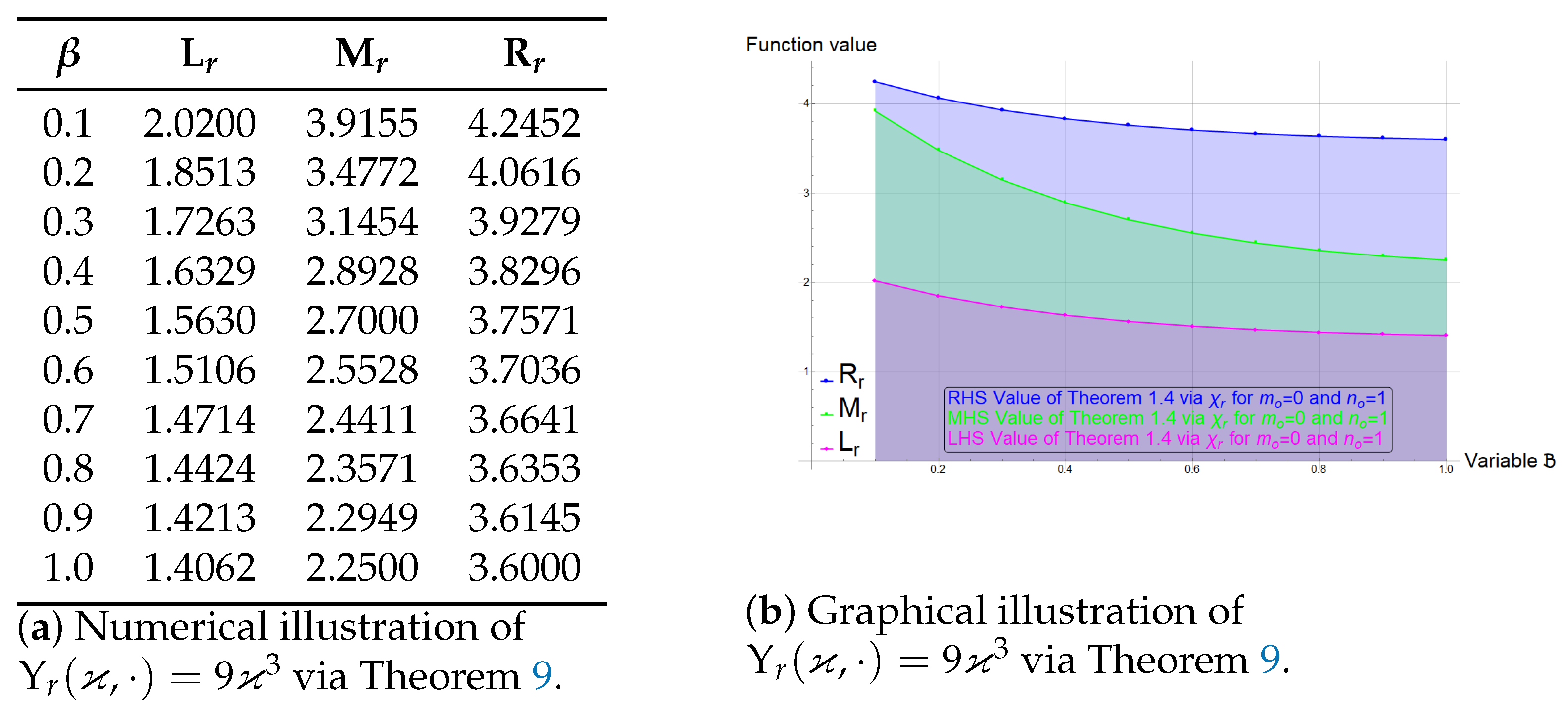
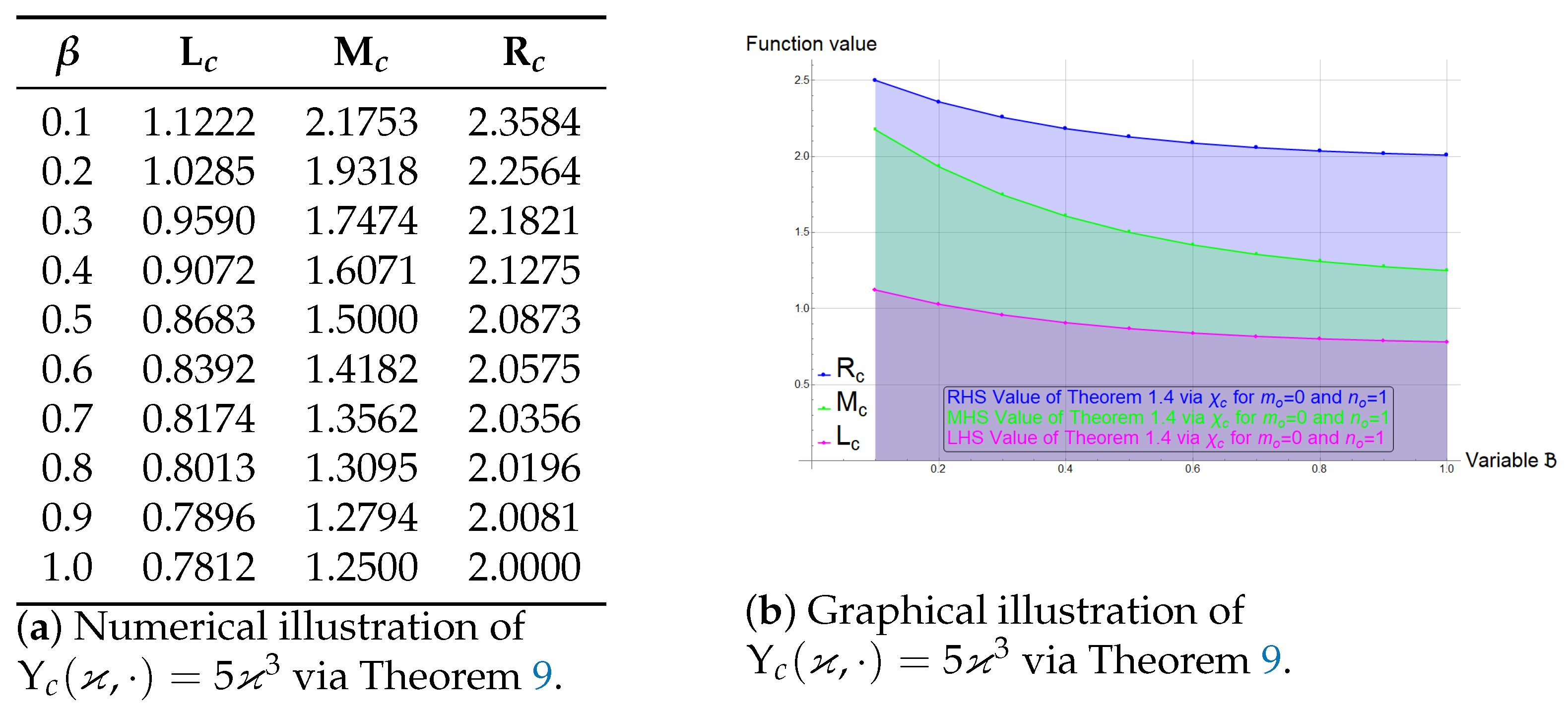
Consider the fractional Hermite-Hadamard’s inequalities via Riemann-Liouville integral operators of order $\beta >0$, for center-radius interval-valued superquadratic stochastic processes from Theorem 9:

$$\begin{array}{cc}\hfill & {\rm Y}\left({\displaystyle \frac{{\mathfrak{s}}_o+{\mathfrak{t}}_o}{2}},.\right)+{\displaystyle \frac{\beta }{2{({\mathfrak{t}}_o-{\mathfrak{s}}_o)}^{\beta }}}{\int }_{{\mathfrak{s}}_o}^{{\mathfrak{t}}_o}{\rm Y}\left(|{\displaystyle \frac{{\mathfrak{s}}_o+{\mathfrak{t}}_o}{2}}-\varkappa |,.\right)({({\mathfrak{t}}_o-\varkappa )}^{\beta -1}+{(\varkappa -{\mathfrak{s}}_o)}^{\beta -1})d\varkappa \hfill \\ \hfill & {⪯}_c^r{\displaystyle \frac{\Gamma (1+\beta )}{2{({\mathfrak{t}}_o-{\mathfrak{s}}_o)}^{\beta }}}\left({\mathrm{I}}_{{{\mathfrak{s}}_o}^{+}}^{\beta }{\rm Y}({\mathfrak{t}}_o,.)+{\mathrm{I}}_{{{\mathfrak{t}}_o}^{-}}^{\beta }{\rm Y}({\mathfrak{s}}_o,.)\right){⪯}_c^r{\displaystyle \frac{{\rm Y}({\mathfrak{s}}_o,.)+{\rm Y}({\mathfrak{t}}_o,.)}{2}}\hfill \\ \hfill & -{\displaystyle \frac{\beta }{2{({\mathfrak{t}}_o-{\mathfrak{s}}_o)}^{\beta }}}{\int }_{{\mathfrak{s}}_o}^{{\mathfrak{t}}_o}\left(\left({\displaystyle \frac{\varkappa -{\mathfrak{s}}_o}{{\mathfrak{t}}_o-{\mathfrak{s}}_o}}\right){\rm Y}({\mathfrak{t}}_o-\varkappa ,.)+\left({\displaystyle \frac{{\mathfrak{t}}_o-\varkappa }{{\mathfrak{t}}_o-{\mathfrak{s}}_o}}\right){\rm Y}(\varkappa -{\mathfrak{s}}_o,.)\right)\hfill \\ \hfill & \times ({({\mathfrak{t}}_o-\varkappa )}^{\beta -1}+{(\varkappa -{\mathfrak{s}}_o)}^{\beta -1})d\varkappa ,\hfill \end{array}$$

(92)

The inequality (104) can also be written in the center-radius interval form as

$$\begin{array}{cc}\hfill & \langle {{\rm Y}}_c\left({\displaystyle \frac{{\mathfrak{s}}_o+{\mathfrak{t}}_o}{2}},.\right)+{\displaystyle \frac{\beta }{2{({\mathfrak{t}}_o-{\mathfrak{s}}_o)}^{\beta }}}{\int }_{{\mathfrak{s}}_o}^{{\mathfrak{t}}_o}{{\rm Y}}_c\left(|{\displaystyle \frac{{\mathfrak{s}}_o+{\mathfrak{t}}_o}{2}}-\varkappa |,.\right)({({\mathfrak{t}}_o-\varkappa )}^{\beta -1}+{(\varkappa -{\mathfrak{s}}_o)}^{\beta -1})d\varkappa ,\hfill \\ & {{\rm Y}}_r\left({\displaystyle \frac{{\mathfrak{s}}_o+{\mathfrak{t}}_o}{2}},.\right)+{\displaystyle \frac{\beta }{2{({\mathfrak{t}}_o-{\mathfrak{s}}_o)}^{\beta }}}{\int }_{{\mathfrak{s}}_o}^{{\mathfrak{t}}_o}{{\rm Y}}_r\left(|{\displaystyle \frac{{\mathfrak{s}}_o+{\mathfrak{t}}_o}{2}}-\varkappa |,.\right)({({\mathfrak{t}}_o-\varkappa )}^{\beta -1}+{(\varkappa -{\mathfrak{s}}_o)}^{\beta -1})d\varkappa \rangle \hfill \\ \hfill & {⪯}_c^r〈{\displaystyle \frac{\Gamma (1+\beta )}{2{({\mathfrak{t}}_o-{\mathfrak{s}}_o)}^{\beta }}}\left({\mathrm{I}}_{{{\mathfrak{s}}_o}^{+}}^{\beta }{{\rm Y}}_c({\mathfrak{t}}_o,.)+{\mathrm{I}}_{{{\mathfrak{t}}_o}^{-}}^{\beta }{{\rm Y}}_c({\mathfrak{s}}_o,.)\right),{\displaystyle \frac{\Gamma (1+\beta )}{2{({\mathfrak{t}}_o-{\mathfrak{s}}_o)}^{\beta }}}\left({\mathrm{I}}_{{{\mathfrak{s}}_o}^{+}}^{\beta }{{\rm Y}}_r({\mathfrak{t}}_o,.)+{\mathrm{I}}_{{{\mathfrak{t}}_o}^{-}}^{\beta }{{\rm Y}}_r({\mathfrak{s}}_o,.)\right)〉\hfill \\ \hfill & {⪯}_c^r\langle {\displaystyle \frac{{{\rm Y}}_c({\mathfrak{s}}_o,.)+{{\rm Y}}_c({\mathfrak{t}}_o,.)}{2}}-{\displaystyle \frac{\beta }{2{({\mathfrak{t}}_o-{\mathfrak{s}}_o)}^{\beta }}}{\int }_{{\mathfrak{s}}_o}^{{\mathfrak{t}}_o}(\left({\displaystyle \frac{\varkappa -{\mathfrak{s}}_o}{{\mathfrak{t}}_o-{\mathfrak{s}}_o}}\right){{\rm Y}}_c({\mathfrak{t}}_o-\varkappa ,.)\hfill \\ \hfill & +\left({\displaystyle \frac{{\mathfrak{t}}_o-\varkappa }{{\mathfrak{t}}_o-{\mathfrak{s}}_o}}\right){{\rm Y}}_c(\varkappa -{\mathfrak{s}}_o,.))({({\mathfrak{t}}_o-\varkappa )}^{\beta -1}+{(\varkappa -{\mathfrak{s}}_o)}^{\beta -1})d\varkappa ,\hfill \\ & {\displaystyle \frac{{{\rm Y}}_r({\mathfrak{s}}_o,.)+{{\rm Y}}_r({\mathfrak{t}}_o,.)}{2}}-{\displaystyle \frac{\beta }{2{({\mathfrak{t}}_o-{\mathfrak{s}}_o)}^{\beta }}}{\int }_{{\mathfrak{s}}_o}^{{\mathfrak{t}}_o}(\left({\displaystyle \frac{\varkappa -{\mathfrak{s}}_o}{{\mathfrak{t}}_o-{\mathfrak{s}}_o}}\right){{\rm Y}}_r({\mathfrak{t}}_o-\varkappa ,.)\hfill \\ \hfill & +\left({\displaystyle \frac{{\mathfrak{t}}_o-\varkappa }{{\mathfrak{t}}_o-{\mathfrak{s}}_o}}\right){{\rm Y}}_r(\varkappa -{\mathfrak{s}}_o,.))({({\mathfrak{t}}_o-\varkappa )}^{\beta -1}+{(\varkappa -{\mathfrak{s}}_o)}^{\beta -1})d\varkappa \rangle .\hfill \end{array}$$

(93)

According to Definition 9, the result (93) can be written as

$$\begin{array}{cc}\hfill & {{\rm Y}}_c\left({\displaystyle \frac{{\mathfrak{s}}_o+{\mathfrak{t}}_o}{2}},.\right)+{\displaystyle \frac{\beta }{2{({\mathfrak{t}}_o-{\mathfrak{s}}_o)}^{\beta }}}{\int }_{{\mathfrak{s}}_o}^{{\mathfrak{t}}_o}{{\rm Y}}_c\left(|{\displaystyle \frac{{\mathfrak{s}}_o+{\mathfrak{t}}_o}{2}}-\varkappa |,.\right)({({\mathfrak{t}}_o-\varkappa )}^{\beta -1}+{(\varkappa -{\mathfrak{s}}_o)}^{\beta -1})d\varkappa \hfill \\ \hfill & \le {\displaystyle \frac{\Gamma (1+\beta )}{2{({\mathfrak{t}}_o-{\mathfrak{s}}_o)}^{\beta }}}\left({\mathrm{I}}_{{{\mathfrak{s}}_o}^{+}}^{\beta }{{\rm Y}}_c({\mathfrak{t}}_o,.)+{\mathrm{I}}_{{{\mathfrak{t}}_o}^{-}}^{\beta }{{\rm Y}}_c({\mathfrak{s}}_o,.)\right)\hfill \\ \hfill & \le {\displaystyle \frac{{{\rm Y}}_c({\mathfrak{s}}_o,.)+{{\rm Y}}_c({\mathfrak{t}}_o,.)}{2}}-{\displaystyle \frac{\beta }{2{({\mathfrak{t}}_o-{\mathfrak{s}}_o)}^{\beta }}}{\int }_{{\mathfrak{s}}_o}^{{\mathfrak{t}}_o}(\left({\displaystyle \frac{\varkappa -{\mathfrak{s}}_o}{{\mathfrak{t}}_o-{\mathfrak{s}}_o}}\right){{\rm Y}}_c({\mathfrak{t}}_o-\varkappa ,.)\hfill \\ \hfill & +\left({\displaystyle \frac{{\mathfrak{t}}_o-\varkappa }{{\mathfrak{t}}_o-{\mathfrak{s}}_o}}\right){{\rm Y}}_c(\varkappa -{\mathfrak{s}}_o,.))({({\mathfrak{t}}_o-\varkappa )}^{\beta -1}+{(\varkappa -{\mathfrak{s}}_o)}^{\beta -1})d\varkappa ,\hfill \end{array}$$

(94)

and

$$\begin{array}{cc}\hfill & {{\rm Y}}_r\left({\displaystyle \frac{{\mathfrak{s}}_o+{\mathfrak{t}}_o}{2}},.\right)+{\displaystyle \frac{\beta }{2{({\mathfrak{t}}_o-{\mathfrak{s}}_o)}^{\beta }}}{\int }_{{\mathfrak{s}}_o}^{{\mathfrak{t}}_o}{{\rm Y}}_r\left(|{\displaystyle \frac{{\mathfrak{s}}_o+{\mathfrak{t}}_o}{2}}-\varkappa |,.\right)({({\mathfrak{t}}_o-\varkappa )}^{\beta -1}+{(\varkappa -{\mathfrak{s}}_o)}^{\beta -1})d\varkappa \hfill \\ \hfill & \le {\displaystyle \frac{\Gamma (1+\beta )}{2{({\mathfrak{t}}_o-{\mathfrak{s}}_o)}^{\beta }}}\left({\mathrm{I}}_{{{\mathfrak{s}}_o}^{+}}^{\beta }{{\rm Y}}_r({\mathfrak{t}}_o,.)+{\mathrm{I}}_{{{\mathfrak{t}}_o}^{-}}^{\beta }{{\rm Y}}_r({\mathfrak{s}}_o,.)\right)\hfill \\ \hfill & \le {\displaystyle \frac{{{\rm Y}}_r({\mathfrak{s}}_o,.)+{{\rm Y}}_r({\mathfrak{t}}_o,.)}{2}}-{\displaystyle \frac{\beta }{2{({\mathfrak{t}}_o-{\mathfrak{s}}_o)}^{\beta }}}{\int }_{{\mathfrak{s}}_o}^{{\mathfrak{t}}_o}(\left({\displaystyle \frac{\varkappa -{\mathfrak{s}}_o}{{\mathfrak{t}}_o-{\mathfrak{s}}_o}}\right){{\rm Y}}_r({\mathfrak{t}}_o-\varkappa ,.)\hfill \\ & +\left({\displaystyle \frac{{\mathfrak{t}}_o-\varkappa }{{\mathfrak{t}}_o-{\mathfrak{s}}_o}}\right){{\rm Y}}_r(\varkappa -{\mathfrak{s}}_o,.))({({\mathfrak{t}}_o-\varkappa )}^{\beta -1}+{(\varkappa -{\mathfrak{s}}_o)}^{\beta -1})d\varkappa .\hfill \end{array}$$

(95)

First considering (94) and setting ${\mathfrak{s}}_o=1$, and ${\mathfrak{t}}_o={\displaystyle \frac{\mathfrak{p}\left(\varkappa \right)}{\mathfrak{q}\left(\varkappa \right)}}$, we obtain

$$\begin{array}{cc}\hfill & {{\rm Y}}_c\left({\displaystyle \frac{\mathfrak{q}\left(\varkappa \right)+\mathfrak{p}\left(\varkappa \right)}{2\mathfrak{q}\left(\varkappa \right)}},.\right)+{\displaystyle \frac{\beta }{2{\left(\frac{\mathfrak{p}\left(\varkappa \right)}{\mathfrak{q}\left(\varkappa \right)}-1\right)}^{\beta }}}{\int }_1^{{\displaystyle \frac{\mathfrak{p}\left(\varkappa \right)}{\mathfrak{q}\left(\varkappa \right)}}}\left({\left({\displaystyle \frac{\mathfrak{p}\left(\varkappa \right)}{\mathfrak{q}\left(\varkappa \right)}}-\varkappa \right)}^{\beta -1}+{(\varkappa -1)}^{\beta -1}\right)\hfill \\ \hfill & {{\rm Y}}_c\left(|{\displaystyle \frac{\mathfrak{q}\left(\varkappa \right)+\mathfrak{p}\left(\varkappa \right)}{2\mathfrak{q}\left(\varkappa \right)}}-\varkappa |,.\right)d\varkappa \le {\displaystyle \frac{\Gamma (1+\beta )}{2{\left(\frac{\mathfrak{p}\left(\varkappa \right)}{\mathfrak{q}\left(\varkappa \right)}-1\right)}^{\beta }}}\left(\left({\mathrm{I}}_{1^{+}}^{\beta }{{\rm Y}}_c\right)\left({\displaystyle \frac{\mathfrak{p}\left(\varkappa \right)}{\mathfrak{q}\left(\varkappa \right)}},.\right)+\left({\mathrm{I}}_{{{\displaystyle \frac{\mathfrak{p}\left(\varkappa \right)}{\mathfrak{q}\left(\varkappa \right)}}}^{-}}^{\beta }{{\rm Y}}_c\right)(1,.)\right)\hfill \\ \hfill & \le {\displaystyle \frac{{{\rm Y}}_c(1,.)+{{\rm Y}}_c\left(\frac{\mathfrak{p}\left(\varkappa \right)}{\mathfrak{q}\left(\varkappa \right)},.\right)}{2}}-{\displaystyle \frac{\beta }{2{\left(\frac{\mathfrak{p}\left(\varkappa \right)}{\mathfrak{q}\left(\varkappa \right)}-1\right)}^{\beta +1}}}{\int }_1^{{\displaystyle \frac{\mathfrak{p}\left(\varkappa \right)}{\mathfrak{q}\left(\varkappa \right)}}}((\varkappa -1){{\rm Y}}_c\left({\displaystyle \frac{\mathfrak{p}\left(\varkappa \right)}{\mathfrak{q}\left(\varkappa \right)}}-\varkappa ,.\right)\hfill \\ \hfill & +\left({\displaystyle \frac{\mathfrak{p}\left(\varkappa \right)}{\mathfrak{q}\left(\varkappa \right)}}-\varkappa \right){{\rm Y}}_c(\varkappa -1,.))\left({\left({\displaystyle \frac{\mathfrak{p}\left(\varkappa \right)}{\mathfrak{q}\left(\varkappa \right)}}-\varkappa \right)}^{\beta -1}+{(\varkappa -1)}^{\beta -1}\right)d\varkappa ,\hfill \end{array}$$

since ${{\rm Y}}_c(1,.)=0$, we have

$$\begin{array}{cc}\hfill & {{\rm Y}}_c\left({\displaystyle \frac{\mathfrak{q}\left(\varkappa \right)+\mathfrak{p}\left(\varkappa \right)}{2\mathfrak{q}\left(\varkappa \right)}},.\right)+{\displaystyle \frac{\beta }{2{\left(\frac{\mathfrak{p}\left(\varkappa \right)}{\mathfrak{q}\left(\varkappa \right)}-1\right)}^{\beta }}}{\int }_1^{{\displaystyle \frac{\mathfrak{p}\left(\varkappa \right)}{\mathfrak{q}\left(\varkappa \right)}}}\left({\left({\displaystyle \frac{\mathfrak{p}\left(\varkappa \right)}{\mathfrak{q}\left(\varkappa \right)}}-\varkappa \right)}^{\beta -1}+{(\varkappa -1)}^{\beta -1}\right)\hfill \\ \hfill & \times {{\rm Y}}_c\left(|{\displaystyle \frac{\mathfrak{q}\left(\varkappa \right)+\mathfrak{p}\left(\varkappa \right)}{2\mathfrak{q}\left(\varkappa \right)}}-\varkappa |,.\right)d\varkappa \le {\displaystyle \frac{\Gamma (1+\beta )}{2{\left(\frac{\mathfrak{p}\left(\varkappa \right)}{\mathfrak{q}\left(\varkappa \right)}-1\right)}^{\beta }}}\left(\left({\mathrm{I}}_{1^{+}}^{\beta }{{\rm Y}}_c\right)\left({\displaystyle \frac{\mathfrak{p}\left(\varkappa \right)}{\mathfrak{q}\left(\varkappa \right)}},.\right)+\left({\mathrm{I}}_{{{\displaystyle \frac{\mathfrak{p}\left(\varkappa \right)}{\mathfrak{q}\left(\varkappa \right)}}}^{-}}^{\beta }{{\rm Y}}_c\right)(1,.)\right)\hfill \\ \hfill & \le {\displaystyle \frac{{{\rm Y}}_c\left(\frac{\mathfrak{p}\left(\varkappa \right)}{\mathfrak{q}\left(\varkappa \right)},.\right)}{2}}-{\displaystyle \frac{\beta }{2{\left(\frac{\mathfrak{p}\left(\varkappa \right)}{\mathfrak{q}\left(\varkappa \right)}-1\right)}^{\beta +1}}}{\int }_1^{{\displaystyle \frac{\mathfrak{p}\left(\varkappa \right)}{\mathfrak{q}\left(\varkappa \right)}}}\left((\varkappa -1){{\rm Y}}_c\left({\displaystyle \frac{\mathfrak{p}\left(\varkappa \right)}{\mathfrak{q}\left(\varkappa \right)}}-\varkappa ,.\right)+\left({\displaystyle \frac{\mathfrak{p}\left(\varkappa \right)}{\mathfrak{q}\left(\varkappa \right)}}-\varkappa \right){{\rm Y}}_c(\varkappa -1,.)\right)\hfill \\ \hfill & \times \left({\left({\displaystyle \frac{\mathfrak{p}\left(\varkappa \right)}{\mathfrak{q}\left(\varkappa \right)}}-\varkappa \right)}^{\beta -1}+{(\varkappa -1)}^{\beta -1}\right)d\varkappa ,\hfill \end{array}$$

(96)

multiplying (105), both sides by $\mathfrak{q}\left(\varkappa \right)\ge 0$, where $\varkappa \in \Omega$, and then integrating the result on Ω, we obtain

$$\begin{array}{cc}\hfill & {\int }_{\Omega }\mathfrak{q}\left(\varkappa \right){{\rm Y}}_c\left({\displaystyle \frac{\mathfrak{q}\left(\varkappa \right)+\mathfrak{p}\left(\varkappa \right)}{2\mathfrak{q}\left(\varkappa \right)}},.\right)d\mu \left(\varkappa \right)+{\displaystyle \frac{\beta }{2}}{\int }_{\Omega }{\displaystyle \frac{\mathfrak{q}\left(\varkappa \right)}{{\left(\frac{\mathfrak{p}\left(\varkappa \right)}{\mathfrak{q}\left(\varkappa \right)}-1\right)}^{\beta }}}\hfill \\ & \times \left[{\int }_1^{{\displaystyle \frac{\mathfrak{p}\left(\varkappa \right)}{\mathfrak{q}\left(\varkappa \right)}}}\left({\left({\displaystyle \frac{\mathfrak{p}\left(\varkappa \right)}{\mathfrak{q}\left(\varkappa \right)}}-\varkappa \right)}^{\beta -1}+{(\varkappa -1)}^{\beta -1}\right){{\rm Y}}_c\left(|{\displaystyle \frac{\mathfrak{q}\left(\varkappa \right)+\mathfrak{p}\left(\varkappa \right)}{2\mathfrak{q}\left(\varkappa \right)}}-\varkappa |,.\right)d\varkappa \right]d\mu \left(\varkappa \right)\hfill \\ \hfill & \le \Gamma (1+\beta ){\int }_{\Omega }\mathfrak{q}\left(\varkappa \right){\displaystyle \frac{\left[\left({\mathrm{I}}_{1^{+}}^{\beta }{{\rm Y}}_c\right)\left(\frac{\mathfrak{p}\left(\varkappa \right)}{\mathfrak{q}\left(\varkappa \right)},.\right)+\left({\mathrm{I}}_{{\frac{\mathfrak{p}\left(\varkappa \right)}{\mathfrak{q}\left(\varkappa \right)}}^{-}}^{\beta }{{\rm Y}}_c\right)\left(1,.\right)\right]}{2{\left(\frac{\mathfrak{p}\left(\varkappa \right)}{\mathfrak{q}\left(\varkappa \right)}-1\right)}^{\beta }}}d\mu \left(\varkappa \right)\hfill \\ \hfill & \le {\displaystyle \frac{1}{2}}{\int }_{\Omega }\mathfrak{q}\left(\varkappa \right){{\rm Y}}_c\left({\displaystyle \frac{\mathfrak{p}\left(\varkappa \right)}{\mathfrak{q}\left(\varkappa \right)}},.\right)d\mu \left(\varkappa \right)\hfill \\ \hfill & -{\displaystyle \frac{\beta }{2}}{\int }_{\Omega }[{\displaystyle \frac{\mathfrak{q}\left(\varkappa \right)}{{\left(\frac{\mathfrak{p}\left(\varkappa \right)}{\mathfrak{q}\left(\varkappa \right)}-1\right)}^{\beta +1}}}{\int }_1^{{\displaystyle \frac{\mathfrak{p}\left(\varkappa \right)}{\mathfrak{q}\left(\varkappa \right)}}}\left((\varkappa -1){{\rm Y}}_c\left({\displaystyle \frac{\mathfrak{p}\left(\varkappa \right)}{\mathfrak{q}\left(\varkappa \right)}}-\varkappa ,.\right)+\left({\displaystyle \frac{\mathfrak{p}\left(\varkappa \right)}{\mathfrak{q}\left(\varkappa \right)}}-\varkappa \right){{\rm Y}}_c(\varkappa -1,.)\right)\hfill \\ & \times \left({\left({\displaystyle \frac{\mathfrak{p}\left(\varkappa \right)}{\mathfrak{q}\left(\varkappa \right)}}-\varkappa \right)}^{\beta -1}+{(\varkappa -1)}^{\beta -1}\right)d\varkappa ]d\mu \left(\varkappa \right).\hfill \end{array}$$

(97)

Employing the definitions of stochastic divergence, stochastic Hermite–Hadamard divergence and Riemann–Liouville fractional stochastic Hermite–Hadamard divergence, we obtain the following result.

$$\begin{array}{cc}\hfill & {\displaystyle \frac{{SD}_{{{\rm Y}}_c}\left(\frac{1}{2}\mathfrak{q}+\frac{1}{2}\mathfrak{p}\left|\right|\mathfrak{q}\right)}{\Gamma (1+\beta )}}+{\displaystyle \frac{\beta {\tau }_{1_c}}{2\Gamma (1+\beta )}}\le {}^{\beta }SD_{HH}^{{{\rm Y}}_c}\left(\mathfrak{p}\right|\left|\mathfrak{q}\right)\le {\displaystyle \frac{{SD}_{{{\rm Y}}_c}\left(\mathfrak{p}\right|\left|\mathfrak{q}\right)}{2\Gamma (1+\beta )}}-{\displaystyle \frac{\beta {\tau }_{2_c}}{2\Gamma (1+\beta )}}.\hfill \end{array}$$

(98)

Next considering (94) and moving in the same fashion as for ${{\rm Y}}_c$, we determine that

$$\begin{array}{cc}\hfill & {\displaystyle \frac{{SD}_{{{\rm Y}}_r}\left(\frac{1}{2}\mathfrak{q}+\frac{1}{2}\mathfrak{p}\left|\right|\mathfrak{q}\right)}{\Gamma (1+\beta )}}+{\displaystyle \frac{\beta {\tau }_{1_r}}{2\Gamma (1+\beta )}}\le {}^{\beta }SD_{HH}^{{{\rm Y}}_r}\left(\mathfrak{p}\right|\left|\mathfrak{q}\right)\le {\displaystyle \frac{{SD}_{{{\rm Y}}_r}\left(\mathfrak{p}\right|\left|\mathfrak{q}\right)}{2\Gamma (1+\beta )}}-{\displaystyle \frac{\beta {\tau }_{2_r}}{2\Gamma (1+\beta )}}.\hfill \end{array}$$

(99)

Again by Definition 9, the inequalities (98) and (99) represent its RHS and can be written as follows:

$$\begin{array}{cc}\hfill & 〈{\displaystyle \frac{{SD}_{{{\rm Y}}_c}\left(\frac{1}{2}\mathfrak{q}+\frac{1}{2}\mathfrak{p}\left|\right|\mathfrak{q}\right)}{\Gamma (1+\beta )}}+{\displaystyle \frac{\beta {\tau }_{1_c}}{2\Gamma (1+\beta )}},{\displaystyle \frac{{SD}_{{{\rm Y}}_r}\left(\frac{1}{2}\mathfrak{q}+\frac{1}{2}\mathfrak{p}\left|\right|\mathfrak{q}\right)}{\Gamma (1+\beta )}}+{\displaystyle \frac{\beta {\tau }_{1_r}}{2\Gamma (1+\beta )}}〉\hfill \\ & {⪯}_c^r〈{}^{\beta }SD_{HH}^{{{\rm Y}}_c}\left(\mathfrak{p}\right|\left|\mathfrak{q}\right),{}^{\beta }SD_{HH}^{{{\rm Y}}_r}\left(\mathfrak{p}\right|\left|\mathfrak{q}\right)〉\hfill \\ & {⪯}_c^r〈{\displaystyle \frac{{SD}_{{{\rm Y}}_c}\left(\mathfrak{p}\right|\left|\mathfrak{q}\right)}{2\Gamma (1+\beta )}}-{\displaystyle \frac{\beta {\tau }_{2_c}}{2\Gamma (1+\beta )}},{\displaystyle \frac{{SD}_{{{\rm Y}}_r}\left(\mathfrak{p}\right|\left|\mathfrak{q}\right)}{2\Gamma (1+\beta )}}-{\displaystyle \frac{\beta {\tau }_{2_r}}{2\Gamma (1+\beta )}}〉.\hfill \end{array}$$

This implies that

$$\begin{array}{cc}\hfill & {\displaystyle \frac{{SD}_{{\rm Y}}\left(\frac{1}{2}\mathfrak{q}+\frac{1}{2}\mathfrak{p}\left|\right|\mathfrak{q}\right)}{\Gamma (1+\beta )}}+{\displaystyle \frac{\beta {\tau }_1}{2\Gamma (1+\beta )}}{⪯}_c^r{}^{\beta }SD_{HH}^{{\rm Y}}\left(\mathfrak{p}\right|\left|\mathfrak{q}\right){⪯}_c^r{\displaystyle \frac{{SD}_{{\rm Y}}\left(\mathfrak{p}\right|\left|\mathfrak{q}\right)}{2\Gamma (1+\beta )}}-{\displaystyle \frac{\beta {\tau }_2}{2\Gamma (1+\beta )}}.\hfill \end{array}$$

Hence the proof. □

Remark 25. 

If we set $\beta =1$, in Theorem 11, we get the result of Theorem 10.

Remark 26. 

If $\underline{{\rm Y}}(\varkappa ,·)=\overline{{\rm Y}}(\varkappa ,·)$ then we attain the fractional Hermite–Hadamard divergence measure for the superquadratic stochastic process.

5.1. Entropy in Theoretical Information Analysis

Entropy, a foundational concept in information theory, quantifies the amount of uncertainty or unpredictability in a set of possible outcomes. The field of information theory itself was pioneered by Claude Shannon in 1948, when he published his landmark paper “A Mathematical Theory of Communication” in the Bell System Technical Journal. In this work, Shannon introduced a mathematical framework for analyzing information, treating it as a measurable entity in communication systems. His key contribution was the concept of entropy, which provides a precise, quantitative measure of information content in probabilistic terms and is typically expressed in bits. Shannon’s entropy made it possible to mathematically describe and analyze relations such as message uncertainty and communication efficiency that were previously understood only intuitively. This breakthrough laid the groundwork for modern digital communication, data compression, cryptography, and even emerging fields like quantum information and machine learning.

5.1.1. Shannon Entropy

For a discrete random variable $\mathrm{A}$ with probability distribution ${\mathbf{p}}_{\mathrm{o}}=({\rho }_1,\dots ,{\rho }_{\mathrm{n}})$, where each ${\rho }_i$ represents the probability that $\mathrm{A}$ takes its i-th possible value, the Shannon entropy is defined as follows:

$$\begin{array}{c}\hfill H\left(\mathrm{A}\right)=-\sum _{i=1}^{\mathrm{n}}{\rho }_{i}ln{\rho }_i.\end{array}$$

(100)

5.1.2. Relative Entropy

The relative entropy of the probability distribution ${\mathbf{p}}_{\mathrm{o}}$ with respect to another distribution ${\mathbf{q}}_{\mathrm{o}}$ is denoted by $H\left({\mathbf{p}}_{\mathrm{o}}|{\mathbf{q}}_{\mathrm{o}}\right)$ and is defined as follows:

$$\begin{array}{c}\hfill H\left({\mathbf{p}}_{\mathrm{o}}|{\mathbf{q}}_{\mathrm{o}}\right)=\sum _{i=1}^{\mathrm{n}}{\rho }_{i}ln{\displaystyle \frac{{\rho }_i}{{\mathfrak{q}}_i}}.\end{array}$$

(101)

Next, we derive estimates for center-radius interval-valued superquadratic stochastic processes using Theorem 7.

Theorem 12. 

Let $\mathrm{A}$ be a random variable with ${\mathit{p}}_{\mathrm{o}}=({\rho }_1,\dots ,{\rho }_{\mathrm{n}}),$ as its probability distribution where ${\rho }_i\ge 0$, for each i, $1\le i\le \mathrm{n}$ and $H_{\mathrm{n}}\left({\mathit{p}}_{\mathrm{o}}\right)=\mathrm{n}$ then

$$\begin{array}{cc}\hfill & 〈0,H\left(\mathrm{A}\right)〉{⪰}_c^r〈0,\sum _{i=1}^{\mathfrak{n}}{\displaystyle \frac{1}{{\rho }_i}}{\left({\rho }_i-H_{\mathrm{n}}\left({\mathit{p}}_{\mathrm{o}}\right)\right)}^{2}ln{\left(|{\rho }_i-H_{\mathrm{n}}\left({\mathit{p}}_{\mathrm{o}}\right)|\right)}^{-1}-H_{\mathrm{n}}^2\left({\mathit{p}}_{\mathrm{o}}\right)ln{H}_{\mathrm{n}}\left({\mathit{p}}_{\mathrm{o}}\right)〉.\hfill \end{array}$$

(102)

Proof. 

Consider the result of Theorem 7, i.e.,

$$\begin{array}{cc}\hfill & {\rm Y}(\widehat{\varkappa },·)+\sum _{i=1}^{\mathfrak{n}}{\beta }_i{\rm Y}\left(\right|{\varkappa }_i-\widehat{\varkappa }|,·){⪯}_c^r\sum _{i=1}^{\mathfrak{n}}{\beta }_i{\rm Y}({\varkappa }_i,·),\hfill \end{array}$$

(103)

We may restate this as

$$\begin{array}{cc}\hfill & 〈{{\rm Y}}_c(\widehat{\varkappa },·),{{\rm Y}}_r(\widehat{\varkappa },·)〉{⪯}_c^r\langle \sum _{i=1}^{\mathfrak{n}}{\beta }_i{{\rm Y}}_c({\varkappa }_i,·)-\sum _{i=1}^{\mathfrak{n}}{\beta }_i{{\rm Y}}_c\left(\right|{\varkappa }_i-\widehat{\varkappa }|,·),\hfill \\ & \sum _{i=1}^{\mathfrak{n}}{\beta }_i{{\rm Y}}_r({\varkappa }_i,·)-\sum _{i=1}^{\mathfrak{n}}{\beta }_i{{\rm Y}}_r\left(\right|{\varkappa }_i-\widehat{\varkappa }|,·)\rangle ,\hfill \end{array}$$

(104)

Based on the inclusion in (104), we deduce that

$$\begin{array}{cc}\hfill & {{\rm Y}}_c(\widehat{\varkappa },·)\le \sum _{i=1}^{\mathfrak{n}}{\beta }_i{{\rm Y}}_c({\varkappa }_i,·)-\sum _{i=1}^{\mathfrak{n}}{\beta }_i{{\rm Y}}_c\left(\right|{\varkappa }_i-\widehat{\varkappa }|,·),\hfill \end{array}$$

(105)

and

$$\begin{array}{cc}\hfill & {{\rm Y}}_r(\widehat{\varkappa },·)\le \sum _{i=1}^{\mathfrak{n}}{\beta }_i{{\rm Y}}_r({\varkappa }_i,·)-\sum _{i=1}^{\mathfrak{n}}{\beta }_i{{\rm Y}}_r\left(\right|{\varkappa }_i-\widehat{\varkappa }|,·),\hfill \end{array}$$

(106)

first taking into account (105)

$$\begin{array}{cc}\hfill & {{\rm Y}}_c(\widehat{\varkappa },·)\le \sum _{i=1}^{\mathfrak{n}}{\beta }_i{{\rm Y}}_c({\varkappa }_i,·)-\sum _{i=1}^{\mathfrak{n}}{\beta }_i{{\rm Y}}_c\left(\right|{\varkappa }_i-\widehat{\varkappa }|,·),\hfill \end{array}$$

(107)

setting $\widehat{\varkappa }={\sum }_{i=1}^{\mathfrak{n}}{\beta }_i{\varkappa }_i$, ${\varkappa }_i={\rho }_i$ and ${\beta }_i={\displaystyle \frac{1}{{\rho }_i}}$ in (107), we get

$$\begin{array}{cc}\hfill & \sum _{i=1}^{\mathfrak{n}}{\displaystyle \frac{1}{{\rho }_i}}{{\rm Y}}_c({\rho }_i,·)\le {{\rm Y}}_c\left(H_{\mathrm{n}}\left({\mathbf{p}}_{\mathrm{o}}\right),·\right)+\sum _{i=1}^{\mathfrak{n}}{\displaystyle \frac{1}{{\rho }_i}}{{\rm Y}}_c\left(|{\rho }_i-H_{\mathrm{n}}\left({\mathbf{p}}_{\mathrm{o}}\right)|,·\right),\hfill \end{array}$$

(108)

as we use the process ${\rm Y}(\varkappa ,·)=[\underline{{\rm Y}}(\varkappa ,·),\overline{{\rm Y}}(\varkappa ,·)]$. Taking $\underline{{\rm Y}}(\varkappa ,·)=-{\varkappa }^{2}ln\left(\varkappa \right)$ and $\overline{{\rm Y}}(\varkappa ,·)={\varkappa }^{2}ln\left(\varkappa \right)$ then $〈{{\rm Y}}_c(\varkappa ,·),{{\rm Y}}_r(\varkappa ,·)〉=〈0,{\varkappa }^{2}ln\left(\varkappa \right)〉$ therefore setting ${{\rm Y}}_c(\varkappa ,·)=0$ in (108), we get

$$\begin{array}{cc}\hfill & 0\le 0,\hfill \end{array}$$

(109)

similarly considering (106) and setting ${{\rm Y}}_r(\varkappa ,·)={\varkappa }^{2}ln\left(\varkappa \right)$, we get

$$\begin{array}{cc}\hfill & \sum _{i=1}^{\mathfrak{n}}{\rho }_{i}ln{\rho }_i\le H_{\mathrm{n}}^2\left({\mathbf{p}}_{\mathrm{o}}\right)ln{H}_{\mathrm{n}}\left({\mathbf{p}}_{\mathrm{o}}\right)+\sum _{i=1}^{\mathfrak{n}}{\displaystyle \frac{1}{{\rho }_i}}{\left({\rho }_i-H_{\mathrm{n}}\left({\mathbf{p}}_{\mathrm{o}}\right)\right)}^{2}ln\left(|{\rho }_i-H_{\mathrm{n}}\left({\mathbf{p}}_{\mathrm{o}}\right)|\right),\hfill \end{array}$$

(110)

Multiplying both sides of (110) by −1 yields

$$\begin{array}{cc}\hfill & H\left(\mathrm{A}\right)\ge \sum _{i=1}^{\mathfrak{n}}{\displaystyle \frac{1}{{\rho }_i}}{\left({\rho }_i-H_{\mathrm{n}}\left({\mathbf{p}}_{\mathrm{o}}\right)\right)}^{2}ln{\left(|{\rho }_i-H_{\mathrm{n}}\left({\mathbf{p}}_{\mathrm{o}}\right)|\right)}^{-1}-H_{\mathrm{n}}^2\left({\mathbf{p}}_{\mathrm{o}}\right)ln{H}_{\mathrm{n}}\left({\mathbf{p}}_{\mathrm{o}}\right),\hfill \end{array}$$

(111)

The inequalities (109) and (111) imply that

$$\begin{array}{cc}\hfill & 〈0,H\left(\mathrm{A}\right)〉{⪰}_c^r〈0,\sum _{i=1}^{\mathfrak{n}}{\displaystyle \frac{1}{{\rho }_i}}{\left({\rho }_i-H_{\mathrm{n}}\left({\mathbf{p}}_{\mathrm{o}}\right)\right)}^{2}ln{\left(|{\rho }_i-H_{\mathrm{n}}\left({\mathbf{p}}_{\mathrm{o}}\right)|\right)}^{-1}-H_{\mathrm{n}}^2\left({\mathbf{p}}_{\mathrm{o}}\right)ln{H}_{\mathrm{n}}\left({\mathbf{p}}_{\mathrm{o}}\right)〉,\hfill \end{array}$$

(112)

Hence the proof. □

6. Complexity and Implementation

To provide a clearer sense of computational feasibility, we supplement our theoretical discussion with empirical timing benchmarks. The symbolic routines, particularly those used to generate the data and plots in all figures, were executed using Mathematica 11.3 on a standard workstation (Intel Core i7, 16 GB RAM). The wall-clock times recorded for a representative set of computations range from approximately 0.08 s to 2.77 s, depending on the complexity of the symbolic integration and plotting tasks. These timings confirm that the core routines, despite their symbolic nature, remain tractable and efficient in practice. For reproducibility, we have also provided a link “https://github.com/dawoodpk1947/fractal-and--fractional-time-calculation-for-computation.git (accessed on 30 May 2025)” to the accompanying notebook that documents these timing results and illustrates the computation process in detail.

7. Conclusions

In this paper, we introduced a novel class of interval-valued superquadratic stochastic processes and established several integral Jensen- and Hermite–Hadamard-type inequalities, including their fractional counterparts, under the center-radius total order relation between intervals. These findings were supported by both graphical and numerical evidence, and their relevance was further extended to information theory through the construction of new stochastic divergence measures via interval calculus.

This work opens up several promising avenues for future research. In particular, the framework developed here can be extended to derive further integral inequalities for center-radius ordered interval-valued superquadratic stochastic processes using a variety of fractional operators, such as the (k-p)-fractional integrals, k-fractional integrals, Katugampola fractional integrals, generalized Riemann–Liouville fractional integrals, $\psi$-Riemann–Liouville fractional integrals, and conformable fractional integrals, including new classes of interval-valued stochastic processes such as h-superquadratic stochastic processes, (P, m) superquadratic–stochastic processes, and harmonic superquadratic stochastic processes. All of these can be defined and analyzed within this framework. The foundational results established in this work are expected to serve as a basis for such advancements and to stimulate further developments in the theory of stochastic processes and their applications in uncertainty modeling and information theory.