On Polynomial φ-Contractions with Applications to Fractional Logistic Growth Equations

Abstract

In this article, we introduce and study a novel class of polynomial $\phi$-contractions, which simultaneously generalizes classical polynomial contractions and $\phi$-contractions within a unified framework. We establish generalized fixed point theorems that encompass some results in the existing literature. Furthermore, we derive explicit error estimates and convergence rates for the associated Picard iteration, providing practical insights into the speed of convergence. Several illustrative examples, including higher-degree polynomial contractions, demonstrate the scope and applicability of our results. As an application, we prove existence and uniqueness results for solutions of a class of fractional logistic growth equations, highlighting the relevance of our theoretical contributions to nonlinear analysis and applied mathematics.

1. Introduction

Fixed point theory is a cornerstone of nonlinear analysis, with far-reaching applications in differential equations, optimization, game theory, dynamical systems, and beyond. Among its foundational results is the Banach contraction principle (BCP), established by Banach [1], which guarantees that every contraction mapping on a complete metric space has exactly one fixed point. The BCP not only provides a constructive method for approximating fixed points via Picard iterations but also serves as a prototype for numerous generalizations (for some recent extensions, see [2,3,4,5,6,7] and references therein).

The first significant generalization of BCP was obtained by Rakotch [8] in 1962, replacing the Lipschitz constant $\lambda$ of the contraction condition with a decreasing function $\phi$: $[0,\infty )\to [0,1]$ such that $\phi \left(t\right)<t$ for all $t>0$. Subsequently, Browder [9] introduced a more general definition in 1968 by replacing the right-hand side of the Banach contraction condition with a nonlinear control function $\phi$: $[0,\infty )\to [0,\infty )$, assumed to be non-decreasing, right-continuous, and satisfying $\phi \left(t\right)<t$ for $t>0$. Boyd and Wong [10] further extended Browder’s definition in 1969, observing that it suffices to assume only the right upper semi-continuity of $\phi$, i.e.,

$$\underset{s\to t^{+}}{lim\; sup}\phi \left(s\right)\le \phi \left(t\right)\mathrm{for}\mathrm{all}t\in {\mathbb{R}}_{+}.$$

Another variant was proposed by Matkowski [11] in 1975, who replaced the continuity assumption with the condition:

$$\underset{n\to \infty }{lim}{\phi }^n\left(t\right)=0\mathrm{for}\mathrm{all}t>0,$$

where such functions are known in the literature as comparison functions. The class of Matkowski contractions is strictly broader than Browder’s contraction (see Proposition 2 and Example 2 in [12]). An alternative weakening of Browder’s condition requires

$$\sum _{n=0}^{\infty }{\phi }^n\left(t\right)<\infty \mathrm{for}\mathrm{all}t>0,$$

where such functions are termed $\left(c\right)$-comparison functions (see [13,14]). A detailed comparison of these definitions can be found in the works of Jachymski and coauthors (see [12,15,16,17]). Recently, Jleli et al. [18] introduced the notion of polynomial contractions for self-mappings on a complete metric space $(X,d)$, leading to new fixed point theorems that significantly broaden the applicability of the BCP.

This paper extends the results of Jleli et al. (2025) [18] within the framework of Browder’s (1968) $\phi$-contractions, where $\phi$ is non-decreasing and satisfies:

$$\sum _{n=0}^{\infty }{\left({\phi }^n\left(t\right)\right)}^{1/j}<\infty \mathrm{for}\mathrm{all}t>0\mathrm{and}j=1,2,\dots ,k.$$

Our key innovation is a new polynomial $\phi$-contraction condition that incorporates both polynomial terms and iterated $\phi$-functions, enabling a more flexible analysis of fixed point problems in metric spaces.

At the conclusion of this introductory section, we outline the organization of the paper as follows. Section 2 presents the necessary mathematical preliminaries, including foundational definitions and results that will be used throughout the paper. In Section 3, we introduce polynomial $\phi$-contractions (Definition 4), a flexible class of mappings unifying polynomial terms and iterated $\phi$-functions, and present our main theoretical advances, Theorem 3 (existence/uniqueness of fixed points for continuous mappings) and Theorem 4 (extension to Picard-continuous mappings), supported by numerical examples and convergence analysis (Theorems 5 and 6) with graphical illustrations. Corollaries deriving from these theorems highlight their broader implications. Section 4 demonstrates the applicability of our results by solving a fractional Caputo logistic growth equation, where Theorem 7 guarantees a unique continuous solution, bridging abstract theory with practical differential equations. Finally, in Section 5, we summarize our contributions and suggest potential directions for future research.

2. Mathematical Preliminaries

This section presents key definitions and foundational results from fixed point theory, with an emphasis on polynomial contraction mappings as introduced by Jleli et al. [18]. We focus on concepts essential for the subsequent advancement of this theory.

Consider a function $\phi$: $[0,\infty )\to [0,\infty )$ that is non-decreasing and satisfies

$$\sum _{n=0}^{\infty }{\phi }^n\left(t\right)<\infty ,\mathrm{for}\mathrm{all}t>0,$$

where ${\phi }^n$ refers to the function $\phi$ iterated n times. Functions of this type are termed $\left(c\right)$-comparison functions and are used to define generalized contractive conditions that extend the classical notion of contraction. Let us denote such functions by $\Phi$.

Remark 1. 

The condition ${\sum }_{n=0}^{\infty }{\phi }^n\left(t\right)<\infty$ implies that ${\phi }^n\left(t\right)$ converges to zero as $n\to \infty$, thereby ensuring the convergence of iterative methods.

Lemma 1 

([14]). If $\phi \in \Phi$, then

• $\phi \left(t\right)<t,$ for each $t>0$,
• $\phi \left(0\right)=0$,
• φ is continuous at 0.

Definition 1 

([9]). A φ-contraction on a metric space $(X,d)$ is a self-mapping T for which there exists $\phi \in \Phi$ such that

$$d(Tx,Ty)\le \phi \left(d\right(x,y\left)\right),$$

for every $x,y\in X.$

Definition 2 

([18]). A polynomial contraction on a metric space $(X,d)$ is a self-mapping T for which there exist $\lambda \in [0,1)$, a positive integer k, and a class of functions $a_i$$:X\times X\to [0,\infty )$ satisfying

$$\sum _{i=0}^k{a}_i(Tx,Ty)d^i(Tx,Ty)\le \lambda \sum _{i=0}^k{a}_i(x,y)d^i(x,y),\forall x,y\in X.$$

Utilizing the notion of polynomial contractions, Jleli et al. [18] established fixed point theorems that extend the BCP and provide a broader framework for studying the convergence and uniqueness of fixed points.

Theorem 1 

([18]). Consider the metric space $(X,d)$, which is complete, and a polynomial contraction self-mapping T. Suppose the following requirements are fulfilled:

(i) 

The mapping T is continuous;

(ii) 

For some $j\in \{1,\dots ,k\}$, the coefficient function $a_j$ is uniformly bounded below by a positive constant $A_j$ (i.e., $a_j(x,y)\ge A_j>0,\mathit{for}\mathit{all}x,y\in X$).

Then, T possesses exactly one fixed point $x^{*}$ in X. For arbitrary $x_0\in X$, the recursive process $x_{n+1}=T{x}_n$ yields convergence to $x^{*}$.

Definition 3 

([18]). In a metric space $(X,d)$, a mapping T is Picard-continuous if ${lim}_{n\to \infty }d(T^{n}z,w)$ = $0\Rightarrow {lim}_{n\to \infty }d(T\left(T^{n}z\right),Tw)=0,$ for all $z,w\in X$, where $T^{0}z=z$ and $T^{n+1}z=T\left(T^{n}z\right)$.

Theorem 2 

([18]). Consider the metric space $(X,d)$, which is complete, and a polynomial contraction T. Suppose the following requirements are fulfilled:

(i) 

The mapping T is Picard-continuous;

(ii) 

For some $j\in \{1,\dots ,k\}$, the coefficient function $a_j$ is uniformly bounded below by a positive constant $A_j$ (i.e., $a_j(x,y)\ge A_j>0,\mathit{for}\mathit{all}x,y\in X$).

Then, T possesses exactly one fixed point $x^{*}$ in X. For arbitrary $x_0\in X$, the recursive process $x_{n+1}=T{x}_n$ yields convergence to $x^{*}$.

3. Main Results

To formalize the role of $\phi$-functions in our results, we use $\Psi$ to refer to the class of monotonically increasing mappings $\phi$: $[0,\infty )\to [0,\infty )$ satisfying

$$s\left(t\right)=\sum _{n=0}^{\infty }{\left({\phi }^n\left(t\right)\right)}^{{\displaystyle \frac{1}{j}}}<\infty ,\forall t>0,j=1,2,\dots ,k,$$

where ${\phi }^n$ refers to the function $\phi$ iterated n times. Examples of functions belonging to this class include

${\phi }_1\left(t\right)=kt,k\in (0,1)$, ${\phi }_2\left(t\right)=e^{{\displaystyle \frac{-1}{t}}}$, ${\phi }_3\left(t\right)=t{e}^{-\sqrt{t}}$, and ${\phi }_4\left(t\right)=\left\{\begin{array}{cc}{t}^2\hfill & \mathrm{if}t\le 1,\hfill \\ 0\hfill & \mathrm{if}t>1.\hfill \end{array}\right.$

Remark 2. 

The condition ${\sum }_{n=0}^{\infty }{\left({\phi }^n\left(t\right)\right)}^{{\displaystyle \frac{1}{j}}}<\infty$ implies that ${\sum }_{n=1}^{\infty }{\phi }^n\left(t\right)<\infty$, for all $j=1,2,\dots ,k$ and $t>0$, ensuring that the class Ψ of the functions described above is a subclass of the class of $\left(c\right)$-comparison functions.

3.1. The Family of Polynomial $\phi$-Contractions

We shall define below a novel class of contraction mappings, namely polynomial $\phi$-contractions, which generalize the classical notion and play a central role in our subsequent analysis.

Definition 4. 

A polynomial φ-contraction on a metric space $(X,d)$ is a self-mapping T for which there exist $\phi \in \Psi$, a positive integer k, and a class of functions $a_i$$:X\times X\to [0,\infty )$ such that

$$\sum _{i=0}^k{a}_i(Tx,Ty)d^i(Tx,Ty)\le \phi \left(\sum _{i=0}^k{a}_i(x,y)d^i(x,y)\right),\forall x,y\in X.$$

(1)

Remark 3. 

By choosing the essential functions $a_i$ and φ suitably in Definition 4, one can deduce many contractions, which substantiates that polynomial φ-contractions unify several kinds of contractions existing in the literature.

(a) 

By setting $\phi \left(t\right)=\lambda t$ and $\lambda \in [0,1)$, we deduce polynomial contractions.

(b) 

By choosing $k=1$, $a_0=0$, and $a_1=1$, we obtain φ-contractions.

(c) 

Taking $\phi \left(t\right)=\lambda t$, $\lambda \in [0,1)$, $k=1$, $a_0=0$, and $a_1=1$, we obtain Banach contractions.

Remark 4. 

The functions $a_i(x,y)$ serve as design parameters that tailor the contraction to specific needs.

• They control the type of nonlinearity (e.g., quadratic, cubic).
• They determine convergence rates and stability conditions.
• Their flexibility allows the framework to unify classical and modern contraction theories.

By carefully selecting $a_i(x,y)$, one can balance generality and tractability, making polynomial φ-contractions a powerful tool in nonlinear analysis.

We are now ready to present and demonstrate our principal results. First, we examine the case where the mapping T is continuous.

Theorem 3. 

Let T be a polynomial φ-contraction self-mapping on a complete metric space $(X,d)$. Suppose the following requirements are fulfilled:

(i) 

The mapping T is continuous;

(ii) 

For some $j\in \{1,\dots ,k\}$, the coefficient function $a_j$ is uniformly bounded below by a positive constant $A_j$ (i.e., $a_j(x,y)\ge A_j>0,\mathit{for}\mathit{all}x,y\in X$).

Then, T possesses exactly one fixed point $x^{*}$ in X. For arbitrary $x_0\in X$, the recursive process $x_{n+1}=T{x}_n$ yields convergence to $x^{*}$.

Proof. 

Let $x_0$ be a fixed starting point. Consider the Picard iterates $\left\{x_n\right\}$ associated with T, i.e.,

$$x_{n+1}=T{x}_n,n\ge 0.$$

By the polynomial $\phi$-contraction property of T, for $x=x_{n-1}$ and $y=x_n$, we get

$$\sum _{i=1}^k{a}_i(x_n,x_{n+1})d^i(x_n,x_{n+1})\le \phi \left(\sum _{i=1}^k{a}_i(x_{n-1},x_n)d^i(x_{n-1},x_n)\right).$$

Let $D_n={\sum }_{i=1}^k{a}_i(x_n,x_{n+1})d^i(x_n,x_{n+1})$; the above inequality becomes

$$D_n\le \phi \left(D_{n-1}\right),\mathrm{for}\mathrm{all}n\ge 1.$$

By iteration, we get

$$D_n\le {\phi }^n\left(D_0\right),\mathrm{for}\mathrm{all}n\ge 0.$$

(2)

From condition $\left(ii\right)$, there exists an index j satisfying

$$a_j(x,y)\ge A_j.$$

This ensures that the term $a_j(x_n,x_{n+1})d^j(x_n,x_{n+1})$ in $D_n$ is significant. Specifically,

$$D_n\ge a_j(x_n,x_{n+1})d^j(x_n,x_{n+1})\ge A_j{d}^j(x_n,x_{n+1}).$$

Combining this with (2), we obtain

$$d^j(x_n,x_{n+1})\le {\displaystyle \frac{{\phi }^n\left(D_0\right)}{A_j}}.$$

(3)

Taking the j-th root,

$$d(x_n,x_{n+1})\le {\left({\displaystyle \frac{{\phi }^n\left(D_0\right)}{A_j}}\right)}^{1/j}.$$

For $m>n$, applying the triangle inequality yields

$$\begin{array}{cc}\hfill d(x_n,x_m)\le \sum _{l=n}^{m-1}d(x_l,x_{l+1})& \le {\left({\displaystyle \frac{1}{A_j}}\right)}^{{\displaystyle \frac{1}{j}}}\sum _{l=n}^{m-1}{\left({\phi }^l\left(D_0\right)\right)}^{1/j}\hfill \\ \hfill & ={\left({\displaystyle \frac{1}{A_j}}\right)}^{{\displaystyle \frac{1}{j}}}\left[\sum _{l=0}^{m-1}{\left({\phi }^l\left(D_0\right)\right)}^{1/j}-\sum _{r=0}^{n-1}{\left({\phi }^r\left(D_0\right)\right)}^{1/j}\right].\hfill \end{array}$$

As $\phi \in \Psi$, the series ${\sum }_{l=0}^{\infty }{\left({\phi }^l\left(D_0\right)\right)}^{{\displaystyle \frac{1}{j}}}$ converges. Thus, ${lim}_{m,n\to \infty }d(x_n,x_m)=0$, proving that $\left\{x_n\right\}$ is Cauchy. By completeness, $\left\{x_n\right\}$ converges to x in X, i.e.,

$$\underset{n\to \infty }{lim}d(x_n,x)=0,$$

which implies, through the continuity property of T, that

$$\underset{n\to \infty }{lim}d(x_{n+1},Tx)=\underset{n\to \infty }{lim}d(T{x}_n,Tx)=0.$$

The uniqueness of the limit establishes x as a fixed point. For uniqueness, assume the existence of $x^{*}\in X,x^{*}\ne x$ with $T{x}^{*}=x^{*}$. Then applying (1) to $(x,x^{*})$, gives

$$\sum _{i=1}^k{a}_i(x,x^{*})d^i(x,x^{*})\le \phi \left(\sum _{i=1}^k{a}_i(x,x^{*})d^i(x,x^{*})\right).$$

(4)

Given $d(x,x^{*})>0$ and the existence of j with $a_j(x,x^{*})>0$ (guaranteed by (ii)), we derive the strict positivity ${\sum }_{i=1}^k{a}_i(x,x^{*})d^i(x,x^{*})>0.$ Then, combining (4) with Lemma 1 yields

$$\sum _{i=1}^k{a}_i(x,x^{*})d^i(x,x^{*})<\sum _{i=1}^k{a}_i(x,x^{*})d^i(x,x^{*}),$$

a contradiction, which confirms that x is unique. This completes the proof. □

Remark 5. 

It is worth noting that Theorem 1 can be obtained directly from Theorem 3 by invoking Remark 3 (a).

Remark 6. 

The conditions imposed on the function φ are essential for ensuring the applicability and robustness of the fixed point results derived in this paper.

• Monotonicity of φ: The assumption that is monotonically increasing ensures that smaller values are mapped to smaller values under iteration. This property supports the preservation of a generalized contraction behavior.
• Convergence Requirement ($s\left(t\right)<\infty$): The condition $s\left(t\right)={\sum }_{n=0}^{\infty }{\left({\phi }^n\left(t\right)\right)}^{1/j}<\infty$ ensures that the iterates ${\phi }^n\left(t\right)$ decay to zero sufficiently fast for all $t>0$ and any $j\in \mathbb{N}$. This guarantees the convergence of the Cauchy sequence and the stability of fixed point iterations, as the series’ convergence implies ${\phi }^n\left(t\right)\to 0$ faster than any polynomial in n.

Corollary 1. 

Let T be a polynomial φ-contraction self-mapping on a complete metric space $(X,d)$. Suppose the following requirements are fulfilled:

(i) 

$a_0(x,y)=0$ for all $x,y\in X$;

(ii) 

For each $i\in \{1,\dots ,k\}$, the coefficient function $a_i$ is uniformly bounded above by a positive constant $B_i$ (i.e., $a_i(x,y)\le B_i,\mathrm{for}\mathrm{all}x,y\in X$);

(iii) 

For some $j\in \{1,\dots ,k\}$, the coefficient function $a_j$ is uniformly bounded below by a positive constant $A_j$ (i.e., $a_j(x,y)\ge A_j>0,\mathit{for}\mathit{all}x,y\in X$).

Then, T possesses exactly one fixed point $x^{*}$ in X. For arbitrary $x_0\in X$, the recursive process $x_{n+1}=T{x}_n$ yields convergence to $x^{*}$.

Proof. 

To complete the argument, it suffices to verify the continuity of T. Consider any sequence $\left\{x_n\right\}$ in X that satisfies

$$\underset{n\to \infty }{lim}d(x_n,x)=0,\mathrm{for}\mathrm{some}x\in X.$$

(5)

Applying the contraction property with $x=x_n$ and $y=x$, we obtain

$$\sum _{i=0}^k{a}_i(T{x}_n,Tx)d^i(T{x}_n,Tx)\le \phi \left(\sum _{i=0}^k{a}_i(x_n,x)d^i(x_n,x)\right),n\ge 0.$$

Since $\phi$ is non-decreasing, and making use of conditions $\left(ii\right)$ and $\left(iii\right)$, we get

$$A_j{d}^j(T{x}_n,Tx)\le \phi \left(\sum _{i=0}^k{B}_i{d}^i(x_n,x)\right),n\ge 0.$$

(6)

Taking the limit as $n\to \infty$ in (6) and using (5) and Lemma 1, we have

$$\underset{n\to \infty }{lim}{d}^j(T{x}_n,Tx)=0,$$

which is equivalent to

$$\underset{n\to \infty }{lim}d(T{x}_n,Tx)=0.$$

Therefore, the mapping T is continuous. □

Corollary 1 gives rise to the following result:

Corollary 2. 

Let $(X,d)$ be a complete metric space and $T:X\to X$. Assume that there exist $\phi \in \Psi$, a positive integer k, and a finite sequence ${\left\{a_i\right\}}_{i=1}^k\subset (0,\infty )$ satisfying

$$\sum _{i=0}^k{a}_i{d}^i(Tx,Ty)\le \phi \left(\sum _{i=0}^k{a}_i{d}^i(x,y)\right),\forall x,y\in X.$$

(7)

Then, T possesses exactly one fixed point $x^{*}$. For arbitrary $x_0$ in X, the recursive process $x_{n+1}=T{x}_n$ yields convergence to $x^{*}$.

Remark 7. 

Corollary 2 generalizes the classical φ-contraction result. Setting $k=1$, $a_0=0$, and $a_1=1$ reduces (7) to the standard form:

$$d(Tx,Ty)\le \phi \left(d\right(x,y\left)\right),x,y\in X.$$

Corollary 3. 

Let T be a polynomial φ-contraction self-mapping on a complete metric space $(X,d)$. Suppose the following requirements are fulfilled:

(i) 

$a_0(x,y)=0$ for all $x,y\in X$;

(ii) 

$a_i$ are continuous at $(x,x)$;

(iii) 

For some $j\in \{1,\dots ,k\}$, the coefficient function $a_j$ is uniformly bounded below by a positive constant $A_j$ (i.e., $a_j(x,y)\ge A_j>0,\mathit{for}\mathit{all}x,y\in X$).

Then, T possesses exactly one fixed point $x^{*}$ in X. For arbitrary $x_0\in X$, the recursive process $x_{n+1}=T{x}_n$ yields convergence to $x^{*}$.

Proof. 

To complete the argument, it suffices to verify the continuity of T. Consider any sequence $\left\{x_n\right\}$ in X that satisfies

$$\underset{n\to \infty }{lim}d(x_n,x)=0,\mathrm{for}\mathrm{some}x\in X.$$

(8)

Applying the contraction condition with $x=x_n$ and $y=x$, we get

$$\sum _{i=0}^k{a}_i(T{x}_n,Tx)d^i(T{x}_n,Tx)\le \phi \left(\sum _{i=0}^k{a}_i(x_n,x)d^i(x_n,x)\right),n\ge 0.$$

Making use of (iii), we get

$$A_j{d}^j(T{x}_n,Tx)\le \phi \left(\sum _{i=0}^k{a}_i(x_n,x)d^i(x_n,x)\right),n\ge 0.$$

(9)

Then, taking the limit as $n\to \infty$ in (9) and making use of (8), condition (ii), and Lemma 1, we have

$$\underset{n\to \infty }{lim}{d}^j(T{x}_n,Tx)=0,$$

which is equivalent to

$$\underset{n\to \infty }{lim}d(T{x}_n,Tx)=0.$$

Therefore, the mapping T is continuous. □

As an illustration of the applicability of Theorem 3, we provide the following example. This demonstrates how the theorem operates in a concrete setting and verifies the derived conditions.

Example 1. 

Let $X=[0,1]$ with the usual metric $d(x,y)=|x-y|$. We examine the non-linear mapping $T:X\to X$ given by

$$T\left(x\right)={\displaystyle \frac{x}{1+x}}.$$

T is a continuous mapping on its entire domain. Let $k=1$, $a_0(x,y)=0$, and

$$a_1(x,y)={\displaystyle \frac{1}{1+max\left(\frac{x}{1+x},\frac{y}{1+y}\right)}}.$$

Observe that $a_1(x,y)>{\displaystyle \frac{1}{2}}=A_1>0$. To show that T is a polynomial φ-contraction, we need to verify that

$$a_1(Tx,Ty)d(Tx,Ty)\le \phi \left(a_1(x,y)d(x,y)\right)$$

for some $\phi \in \Psi$. Indeed, taking into account that $|1+x||1+y|\ge 1+max\left({\displaystyle \frac{x}{1+x}},{\displaystyle \frac{y}{1+y}}\right)$ for all $x,y\in X$, we get

$$\begin{array}{cc}\hfill a_1(Tx,Ty)d(Tx,Ty)& ={\displaystyle \frac{1}{1+max\left(\frac{x}{1+2x},\frac{y}{1+2y}\right)}}·{\displaystyle \frac{|x-y|}{|1+x||1+y|}}\hfill \\ \hfill & \le {\displaystyle \frac{1}{1+max\left(\frac{x}{1+2x},\frac{y}{1+2y}\right)}}·{\displaystyle \frac{|x-y|}{1+max\left(\frac{x}{1+x},\frac{y}{1+y}\right)}}\hfill \\ \hfill & ={\displaystyle \frac{1}{1+M}}·{\displaystyle \frac{|x-y|}{1+max\left(\frac{x}{1+x},\frac{y}{1+y}\right)}}\hfill \\ \hfill & =\phi \left(a_1(x,y)d(x,y)\right),\hfill \end{array}$$

where $M=max\left({\displaystyle \frac{x}{1+2x}},{\displaystyle \frac{y}{1+2y}}\right)$ and $\phi \left(t\right)={\displaystyle \frac{1}{1+M}}t$. All requirements of Theorem 3 are satisfied. Consequently, T possesses exactly one fixed point at $x=0$.

The validity of the contraction condition in Example 1 is illustrated in Figure 1.

Remark 8. 

The mapping T given in Example 1 is not a classical Banach contraction. Indeed, contraction-type mappings require the existence of a constant $\lambda <1$. However, the ratio ${\displaystyle \frac{d(Tx,Ty)}{d(x,y)}}$ approaches 1 as $x,y\to 0$. Consequently, for any fixed $\lambda <1$, there exist $x,y$ arbitrarily close to 0 such that ${\displaystyle \frac{d(Tx,Ty)}{d(x,y)}}>\lambda .$ Thus, no single $\lambda <1$ satisfies the contraction condition globally.

Remark 9. 

Using reasoning similar to that in Remark 8, we see that the mapping T in Example 1 fails to be a polynomial contraction with the selected functions $a_i$ for $i=0,1$.

Example 2. 

Consider the metric space $(X,d)$, where $X=[0,1]$ is equipped with the standard Euclidean metric $d(x,y)=|x-y|$. Define the mapping $T:X\to X$ by

$$T\left(x\right)={\displaystyle \frac{x}{2}},\mathit{for}\mathit{all}x\in X.$$

Clearly, T is a continuous self-mapping on X. We shall demonstrate that T is a polynomial φ-contraction of order $k=2$.

Let $a_0,a_1,a_2:X\times X\to [0,\infty )$ be three weight functions defined by

$$a_0(x,y)=0,a_1(x,y)=1+x^2+y^2,a_2(x,y)=|x-y|.$$

These functions are chosen such that $a_1$ depends on the magnitudes of x and y, while $a_2$ captures their separation. The weight functions satisfy

$$a_1(Tx,Ty)=1+{\left({\displaystyle \frac{x}{2}}\right)}^2+{\left({\displaystyle \frac{y}{2}}\right)}^2\le a_1(x,y),a_2(Tx,Ty)={\displaystyle \frac{1}{2}}{a}_2(x,y).$$

The polynomial contraction condition requires

$$\sum _{i=0}^2{a}_i(Tx,Ty)·d^i(Tx,Ty)\le \phi \left(\sum _{i=0}^2{a}_i(x,y)·d^i(x,y)\right),$$

for some function $\phi \in \Psi$. Substituting our expressions, we obtain

$$a_1(Tx,Ty)·d(Tx,Ty)+a_2(Tx,Ty)·d^2(Tx,Ty)\le {\displaystyle \frac{1}{2}}{a}_1(x,y)·d(x,y)+{\displaystyle \frac{1}{8}}{a}_2(x,y)·d^2(x,y).$$

Since ${\displaystyle \frac{1}{8}}<{\displaystyle \frac{1}{2}}$, we may write

$$\sum _{i=1}^2{a}_i(Tx,Ty)·d^i(Tx,Ty)\le {\displaystyle \frac{1}{2}}\left(a_1(x,y)·d(x,y)+a_2(x,y)·d^2(x,y)\right).$$

Thus, defining $\phi \left(t\right)={\displaystyle \frac{1}{2}}t$, we have

$$\sum _{i=1}^2{a}_i(Tx,Ty)·d^i(Tx,Ty)\le \phi \left(\sum _{i=1}^2{a}_i(x,y)·d^i(x,y)\right).$$

The function $\phi \left(t\right)={\displaystyle \frac{1}{2}}t$ belongs to the class Ψ because It is nondecreasing, and for any $t>0$ and $j\in \mathbb{N}$, the series

$$\sum _{n=0}^{\infty }{\left({\phi }^n\left(t\right)\right)}^{1/j}=\sum _{n=0}^{\infty }{\left({\displaystyle \frac{t}{2^n}}\right)}^{1/j}$$

converges (as it is a geometric series with ratio $2^{-1/j}<1$). By Definition 4, T is a polynomial φ-contraction of order 2 with the given weight functions. Consequently, T admits a unique fixed point in X, which is easily verified to be $x=0$.

Theorem 4. 

Consider the metric space $(X,d)$, which is complete, and a polynomial φ-contraction self-mapping T. Suppose the following requirements are fulfilled:

(i) 

The mapping T is Picard-continuous;

(ii) 

For some $j\in \{1,\dots ,k\}$, the coefficient function $a_j$ is uniformly bounded below by a positive constant $A_j$ (i.e., $a_j(x,y)\ge A_j>0,\mathit{for}\mathit{all}x,y\in X$).

Then, T possesses exactly one fixed point $x^{*}$ in X. For arbitrary $x_0\in X$, the recursive process $x_{n+1}=T{x}_n$ yields convergence to $x^{*}$.

Proof. 

Select any initial point $x_0$ in X and construct the iterative sequence $\left\{x_n\right\}$ via

$$x_{n+1}=T{x}_n\mathrm{for}\mathrm{all}n\ge 0.$$

Following the proof of Theorem 3, $\left\{x_n\right\}$ forms a Cauchy sequence. By completeness, $\left\{x_n\right\}$ converges to x in X, i.e.,

$$\underset{n\to \infty }{lim}d(x_n,x)=0.$$

Since T is Picard-continuous, it follows that

$$\underset{n\to \infty }{lim}d(x_{n+1},Tx)=\underset{n\to \infty }{lim}d(T{x}_n,Tx)=0.$$

By the uniqueness of limits, we deduce that

$$Tx=x.$$

The uniqueness of the fixed point follows identically as in Theorem 3. □

Remark 10. 

Notice that, in light of Remark 3 (a), Theorem 2 follows as a consequence of Theorem 4.

Example 3. 

Let $X=[0,1]$ with the usual metric $d(x,y)=|x-y|$. Define $T:X\to X$ by

$$Tx=\left\{\begin{array}{cc}{\displaystyle \frac{1}{3}},\hfill & \mathit{if}0\le x<1,\hfill \\ 0,\hfill & \mathit{if}x=1.\hfill \end{array}\right.$$

Let $a_i:X\times X\to [0,\infty )$ for $i=0,1$ and φ: $[0,\infty )\to [0,\infty )$ be given by

$$a_0(x,y)={\displaystyle \frac{4}{5}}\left(\left|x-\frac{1}{3}\right|+\left|y-\frac{1}{3}\right|\right),a_1(x,y)=1\mathit{and}\phi \left(t\right)={\displaystyle \frac{t}{2}}.$$

We claim that T satisfies the inequality:

$$a_0(Tx,Ty)+d(Tx,Ty)\le \phi \left(a_0(x,y)+d(x,y)\right),\forall x,y\in X,$$

making it a polynomial φ-contraction with $k=1$.

• Case 1: For $x,y\in [0,1)$,

$$a_0(Tx,Ty)+d(Tx,Ty)=a_0\left(\frac{1}{3},\frac{1}{3}\right)+d\left(\frac{1}{3},\frac{1}{3}\right)=0.$$

The inequality $0\le \phi \left(a_0(x,y)+d(x,y)\right)$ holds trivially since φ is non-negative.

• Case 2: For $x\in [0,1)$ and $y=1$,

$$a_0(Tx,Ty)+d(Tx,Ty)=a_0\left(\frac{1}{3},0\right)+d\left(\frac{1}{3},0\right)=\frac{4}{15}+\frac{5}{15}=\frac{9}{15}=\frac{3}{5}.$$

On the other hand, we compute

$$\phi (a_0(x,1)+d(x,1))={\displaystyle \frac{a_0(x,1)+d(x,1)}{2}}={\displaystyle \frac{\frac{4}{5}\left(\left|x-\frac{1}{3}\right|+\frac{2}{3}\right)+|x-1|}{2}}.$$

The inequality can be seen to hold for all $x\in [0,1)$.

• Case 3: For $x=y=1$,

$$a_0(Tx,Ty)+d(Tx,Ty)=a_0(0,0)+d(0,0)=\frac{8}{15},$$

and

$$\phi (a_0(1,1)+d(1,1))={\displaystyle \frac{a_0(1,1)+d(1,1)}{2}}=\frac{8}{15},$$

which confirms the claimed inequality with equality. According to Theorem 4, T possesses a unique fixed point.

The validity of the contraction condition in Example 3 over the entire square $X\times X$ is visualized in Figure 2.

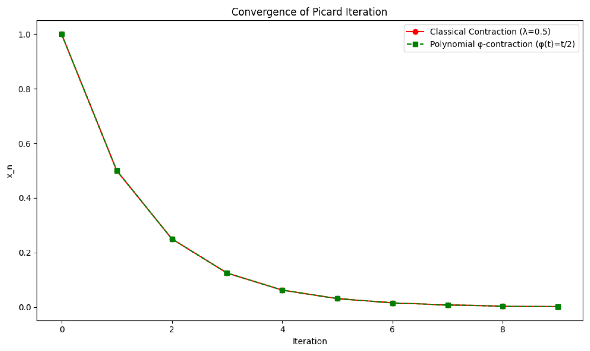
3.2. Convergence Rate and Numerical Verification

We investigate the convergence behavior of the iterative sequences associated with the polynomial-type contractions presented in the main results. We establish two key theorems that provide error estimates and explicit convergence rates, offering a deeper understanding of the efficiency of the proposed mappings. Several corollaries are derived to illustrate the broader implications and special cases of these results. Furthermore, to substantiate the theoretical findings, we present graphical visualizations based on a specific example previously discussed (Examples 1 and 2), highlighting the practical validity and performance of the obtained convergence rates.

Theorem 5 

(Error Estimates for Polynomial $\phi$-contractions). Assuming Theorem 3 holds, the Picard sequence $\left\{z_n\right\}$ satisfies the following error bounds relative to the unique fixed point $z^{*}$:

(i) 

A priori error estimate

$$d(z_n,z^{*})\le {\left({\displaystyle \frac{1}{A_j}}\right)}^{{\displaystyle \frac{1}{j}}}\left[s\left(C\right)-\sum _{r=0}^{n-1}{\left({\phi }^r\left(C\right)\right)}^{1/j}\right],$$

where

• $C={\sum }_{i=0}^k{a}_i(z_0,z_1)d^i(z_0,z_1)$,
• $s\left(t\right)={\sum }_{k=0}^{\infty }{\left({\phi }^k\left(t\right)\right)}^{{\displaystyle \frac{1}{j}}}$,
• and $j\in \{1,2,\dots ,k\}$ with $A_j>0$.

(ii) 

A posteriori error estimate

$$d(z_n,z^{*})\le {\left({\displaystyle \frac{1}{A_j}}\right)}^{{\displaystyle \frac{1}{j}}}\left[s\left(D_{n-1}\right)-{\left(D_{n-1}\right)}^{{\displaystyle \frac{1}{j}}}\right],$$

where $D_{n-1}={\sum }_{i=1}^k{a}_i(z_{n-1},z_n)d^i(z_{n-1},z_n)$.

Proof. 

We build upon the framework established in Theorem 3.

(i)

A priori error estimate: From the contractive condition (Equation (1)) with $x=z_{n-1}$, $y=z_n$, we get

$$\sum _{i=0}^k{a}_i(z_n,z_{n+1})d^i(z_n,z_{n+1})\le {\phi }^n\left(\sum _{i=0}^k{a}_i(z_0,z_1)d^i(z_0,z_1)\right).$$

(10)

As there exist j such that $a_j(z_n,z_{n+1})\ge A_j$, inequality (10) becomes

$$d(z_n,z_{n+1})\le {\left({\displaystyle \frac{1}{A_j}}\right)}^{{\displaystyle \frac{1}{j}}}{\left({\phi }^n\left(\sum _{i=0}^k{a}_i(z_0,z_1)d^i(z_0,z_1)\right)\right)}^{1/j}={\left({\displaystyle \frac{1}{A_j}}\right)}^{{\displaystyle \frac{1}{j}}}{\left({\phi }^n\left(C\right)\right)}^{1/j},$$

where $C={\sum }_{i=0}^k{a}_i(z_0,z_1)d^i(z_0,z_1)$.

For $m>n$, the triangle inequality yields

$$\begin{array}{cc}\hfill d(z_n,z_m)\le \sum _{l=n}^{m-1}d(z_l,z_{l+1})& \le {\left({\displaystyle \frac{1}{A_j}}\right)}^{{\displaystyle \frac{1}{j}}}\sum _{l=n}^{m-1}{\left({\phi }^l\left(C\right)\right)}^{1/j}\hfill \\ \hfill & ={\left({\displaystyle \frac{1}{A_j}}\right)}^{{\displaystyle \frac{1}{j}}}\left[\sum _{l=0}^{m-1}{\left({\phi }^l\left(C\right)\right)}^{1/j}-\sum _{r=0}^{n-1}{\left({\phi }^r\left(C\right)\right)}^{1/j}\right],\hfill \end{array}$$

Taking $m\to \infty$, we obtain the priori error estimate

$$d(z_n,z^{*})\le {\left({\displaystyle \frac{1}{A_j}}\right)}^{{\displaystyle \frac{1}{j}}}\left[s\left(C\right)-\sum _{r=0}^{n-1}{\left({\phi }^r\left(C\right)\right)}^{1/j}\right],$$

(ii)

A Posteriori Error Estimate: Again, from (1) with $x=z_{n-1}$, $y=z_n$, we have

$$\sum _{i=0}^k{a}_i(z_n,z_{n+1})d^i(z_n,z_{n+1})\le \phi \left(\sum _{i=0}^k{a}_i(z_{n-1},z_n)d^i(z_{n-1},z_n)\right).$$

Let $D_n={\sum }_{i=1}^k{a}_i(x_n,x_{n+1})d^i(x_n,x_{n+1})$. The above inequality becomes

$$D_n\le \phi \left(D_{n-1}\right),\mathrm{for}\mathrm{all}n\ge 0,$$

which inductively yields

$$D_{n+k}\le {\phi }^{k+1}\left(D_{n-1}\right),\mathrm{for}\mathrm{all}n\ge 0,k=1,2,\dots$$

(11)

Since there exist j such that $a_j(z_{n+k},z_{n+k+1})\ge A_j$, (11) becomes

$$d(z_{n+k},z_{n+k+1})\le {\left({\displaystyle \frac{1}{A_j}}\right)}^{{\displaystyle \frac{1}{j}}}{\left({\phi }^{k+1}\left(D_{n-1}\right)\right)}^{1/j}.$$

For $m>n$, applying the triangle inequality yield

$$d(z_n,z_m)\le \sum _{l=n}^{m-1}d(z_l,z_{l+1})\le {\left({\displaystyle \frac{1}{A_j}}\right)}^{{\displaystyle \frac{1}{j}}}\sum _{l=1}^{m-n}{\left({\phi }^l\left(D_{n-1}\right)\right)}^{1/j}.$$

Taking $m\to \infty$, we derive the a posteriori error estimate.

$$\begin{array}{cc}\hfill d(z_n,z^{*})\le {\left({\displaystyle \frac{1}{A_j}}\right)}^{{\displaystyle \frac{1}{j}}}\sum _{l=1}^{\infty }{\left({\phi }^l\left(D_{n-1}\right)\right)}^{1/j}& ={\left({\displaystyle \frac{1}{A_j}}\right)}^{{\displaystyle \frac{1}{j}}}\left[\sum _{l=0}^{\infty }{\left({\phi }^l\left(D_{n-1}\right)\right)}^{1/j}-{\left(D_{n-1}\right)}^{{\displaystyle \frac{1}{j}}}\right]\hfill \\ \hfill & ={\left({\displaystyle \frac{1}{A_j}}\right)}^{{\displaystyle \frac{1}{j}}}\left[s\left(D_{n-1}\right)-{\left(D_{n-1}\right)}^{{\displaystyle \frac{1}{j}}}\right],\hfill \end{array}$$

where $s\left(t\right)={\sum }_{k=0}^{\infty }{\left({\phi }^k\left(t\right)\right)}^{{\displaystyle \frac{1}{j}}}.$ This completes the proof.

□

Theorem 6 

(Convergence Rate for Polynomial $\phi$-contractions). Assuming Theorem 3 holds, the Picard sequence $\left\{z_n\right\}$ satisfies the following convergence rate relative to the unique fixed point $z^{*}$:

$$d(z_n,z^{*})\le {\left[{\displaystyle \frac{1}{A_j}}\phi \left(\sum _{i=1}^k{a}_i(z_{n-1},z^{*})d^i(z_{n-1},z^{*})\right)\right]}^{1/j},$$

for some $j\in \{1,2,\dots ,k\}$.

Proof. 

Substituting $x=z_{n-1}$ and $y=z^{*}$ in inequality (1) and applying property $\left(ii\right)$ of Theorem 3, the desired bound follows. □

Corollary 4 

(Error Estimates and Convergence Rate for Polynomial Contractions). Assuming Theorem 1 holds, the Picard sequence $\left\{z_n\right\}$ satisfies the following error bounds relative to the unique fixed point $z^{*}$:

(i) 

A priori error estimate

$$d(z_n,z^{*})\le {\displaystyle \frac{{\lambda }^{n/j}}{1-{\lambda }^{1/j}}}{\left[{\displaystyle \frac{1}{A_j}}\sum _{i=0}^k{a}_i(z_0,z_1)d^i(z_0,z_1)\right]}^{1/j}.$$

(ii) 

A posteriori error estimate

$$d(z_n,z^{*})\le {\displaystyle \frac{{\lambda }^{1/j}}{1-{\lambda }^{1/j}}}{\left[{\displaystyle \frac{1}{A_j}}\sum _{i=1}^k{a}_i(z_{n-1},z_n)d^i(z_{n-1},z_n)\right]}^{1/j}.$$

(iii) 

Convergence rate

$$d(z_n,z^{*})\le {\lambda }^{{\displaystyle \frac{1}{j}}}{\left[{\displaystyle \frac{1}{A_j}}\sum _{i=1}^k{a}_i(z_{n-1},z^{*})d^i(z_{n-1},z^{*})\right]}^{1/j}.$$

Here, $\lambda \in [0,1),j\in \{1,2,\dots ,k\}$ is such that $A_j>0$ is a scaling constant.

Corollary 5 

(Error Estimates and Convergence Rate for $\phi$-contractions). Consider the metric space $(X,d)$ which is complete and let T be a self-mapping such that

$$d(Tx,Ty)\le \phi \left(d\right(x,y\left)\right)\forall x,y\in X,$$

where $\phi \in \Psi$. Then, the Picard iterative sequence $\left\{z_n\right\}$ satisfies the following error bounds relative to the unique fixed point $z^{*}$:

(i) 

A priori error estimate

$$d(z_n,z^{*})\le s\left(d(z_0,z_1)\right)-\sum _{r=0}^{n-1}{\phi }^r\left(d(z_0,z_1)\right).$$

(ii) 

A posteriori error estimate

$$d(z_n,z^{*})\le s\left(d(z_{n-1},z_n)\right)-\left(d(z_{n-1},z_n)\right).$$

(iii) 

Convergence rate

$$d(x_n,z^{*})\le \phi \left(d(z_{n-1},z^{*})\right).$$

where s is a partial sum function of the series ${\sum }_{r=0}^{\infty }{\phi }^r$.

In Example 1, the error at each step of the Picard iteration is measured by $|x_n|$. The sequence generated by the recurrence $x_{n+1}={\displaystyle \frac{x_n}{1+x_n}}$ admits the explicit closed-form solution

$$x_n={\displaystyle \frac{x_0}{1+n{x}_0}}.$$

This expression provides a direct upper bound for the error:

$$\left|x_n\right|\le {\displaystyle \frac{x_0}{1+n{x}_0}}.$$

It follows that the error decreases monotonically with each iteration. Moreover, larger initial values $x_0$ induce a more rapid reduction in the early stages, a phenomenon confirmed by the numerical experiments presented in Figure 3 and Figure 4. These numerical results are in exact agreement with the analytical decay formula and clearly illustrate the monotonic convergence toward the fixed point.

This asymptotic behavior highlights the gradually slowing contraction rate, especially when the initial value $x_0$ is small.

Table 1. Iteration values $x_n$ for various starting points under the mapping $T\left(x\right)={\displaystyle \frac{x}{1+x}}$.

Iteration	${\mathit{x}}_0=1.0$	${\mathit{x}}_0=5.0$	${\mathit{x}}_0=10.0$	${\mathit{x}}_0=20.0$
0	1.000000	5.000000	10.000000	20.000000
1	0.500000	0.833333	0.909091	0.952381
2	0.333333	0.454545	0.476190	0.487805
3	0.250000	0.312500	0.322581	0.327869
4	0.200000	0.238095	0.243902	0.246914
5	0.166667	0.192308	0.196078	0.198020
6	0.142857	0.161290	0.163934	0.165289
7	0.125000	0.138889	0.140845	0.141844
8	0.111111	0.121951	0.123457	0.124224
9	0.100000	0.108696	0.109890	0.110497
10	0.090909	0.098039	0.099010	0.099502
11	0.083333	0.089286	0.090090	0.090498
12	0.076923	0.081967	0.082645	0.082988
13	0.071429	0.075758	0.076336	0.076628
14	0.066667	0.070423	0.070922	0.071174
15	0.062500	0.065789	0.066225	0.066445

presents iteration values computed over 15 steps for several representative initial conditions.

In Example 2, the self-map $T\left(x\right)={\displaystyle \frac{x}{2}}$ on the interval $[0,1]$ was shown to be a polynomial $\phi$-contraction of order $k=2$ with variable coefficient functions:

$$a_1(x,y)=1+x^2+y^2,a_2(x,y)=|x-y|.$$

We analyze how these coefficients influence the convergence behavior of the fixed point iteration $x_{n+1}=T\left(x_n\right)={\displaystyle \frac{x_n}{2}}$ for $x_0\in [0,1]$. The contraction inequality takes the form:

$$a_1(Tx,Ty)·d(Tx,Ty)+a_2(Tx,Ty)·d^2(Tx,Ty)\le \phi \left(a_1(x,y)·d(x,y)+a_2(x,y)·d^2(x,y)\right),$$

where the linear term $a_1(x,y)·d(x,y)$ governs the primary contraction behavior, while the quadratic term $a_2(x,y)·d^2(x,y)$ becomes significant when distances are small, accelerating later-stage convergence. As the iterates approach the fixed point at $x=0$, the coefficients exhibit a limiting behavior:

$$a_1(x_n,0)\to 1,a_2(x_n,0)=x_n\to 0,$$

showing that the convergence becomes dominated by the linear term near the solution. A concrete numerical sequence demonstrates this behavior:

$$x_0=1,x_1=\frac{1}{2},x_2=\frac{1}{4},\dots ,x_n=\frac{1}{2^n},$$

where each iteration halves the distance to the fixed point. The influence of the quadratic term grows as $d(x_n,0)$ decreases, providing faster convergence in later iterations compared to the purely linear contraction. To illustrate the advantages of the generalized polynomial $\phi$-contraction framework, we compare it numerically with the classical Banach contraction. Consider two iterative schemes: the classical Banach contraction defined by $T\left(x\right)=\lambda x$, where $0<\lambda <1$ (here, we take $\lambda =0.5$), and a polynomial $\phi$-contraction given by $T\left(x\right)={\displaystyle \frac{x}{2}}$ but with variable coefficients $a_1(x,y)=1+x^2+y^2$ and $a_2(x,y)=|x-y|$. Applying the Picard iteration $x_{n+1}=T\left(x_n\right)$ from the initial point $x_0=1$, we observe the following numerical results:

In this case, both methods yield identical convergence behavior, as the polynomial $\phi$-contraction simplifies to the classical form (see Figure 5 and

Table 2. Numerical comparison of contraction methods.

Iteration n	Classical Contraction	Polynomial $\mathit{\phi }$-Contraction
0	1.0000	1.0000
1	0.5000	0.5000
2	0.2500	0.2500
3	0.1250	0.1250
4	0.0625	0.0625
5	0.0313	0.0313
6	0.0156	0.0156

). However, the key distinction arises in more general settings where the mapping T is not globally Lipschitz. Unlike the classical Banach contraction, which requires strict Lipschitz conditions, the $\phi$-polynomial framework remains applicable under weaker assumptions. This flexibility is particularly valuable in numerical analysis, where perturbed operators often appear, ensuring convergence in cases where traditional methods fail.

4. Application to Fractional Logistic Equation

Fractional differential equations have emerged as powerful tools for modeling complex systems with memory and hereditary properties, which are often encountered in biological, physical, and engineering applications. Their flexibility in capturing anomalous dynamics makes them particularly suitable for accurately describing real-world phenomena beyond the scope of classical integer-order models. In the recent literature, several studies have advanced fractional modeling techniques to better understand complex diseases like liver fibrosis, breast cancer, and prostate cancer. By introducing new mathematical tools, they enhance the accuracy of biomedical models and deepen insights into dynamic systems (see, for instance, [19,20,21,22,23]).

The fractional logistic growth equation is a generalization of the classical logistic model used to describe population dynamics, biological growth, or the spread of information and diseases. Unlike the standard logistic equation, which assumes instantaneous response and memoryless dynamics, the fractional version introduces memory effects through the use of fractional calculus. Mathematically, the model is described by

$${}^C{D}_t^{\alpha }u\left(t\right)=ru\left(t\right)(1-u\left(t\right)),u\left(0\right)=u_0\in (0,1),$$

where ${}^C{D}_t^{\alpha }$ stands for the Caputo fractional derivative of order $\alpha \in (0,1)$, while $u\left(t\right)$ stands for the population density (or state variable) at time t, $u_0$ is the initial condition constrained to $(0,1)$, and $r>0$ is the growth rate.

This section aims to apply the polynomial $\phi$-contraction theorem (Theorem 3) to the fractional logistic growth equation and prove that it possesses exactly one solution in the space $C[0,L]$ of continuous functions. To this end, we establish the following result:

Theorem 7. 

The fractional logistic growth equation

$${}^C{D}_t^{\alpha }u\left(t\right)=ru\left(t\right)(1-u\left(t\right)),u\left(0\right)=u_0\in (0,1),$$

possesses a unique continuous solution $u\in C[0,L]$ with $0\le u\left(t\right)\le 1$.

Proof. 

The equivalent Volterra integral form of the fractional logistic growth equation is given by

$$u\left(t\right)=u_0+{\displaystyle \frac{r}{\Gamma \left(\alpha \right)}}{\int }_0^t{(t-s)}^{\alpha -1}u\left(s\right)(1-u\left(s\right))ds.$$

We consider the operator T defined on the space $C[0,L]$ by

$$\left(Tu\right)\left(t\right)=u_0+{\displaystyle \frac{r}{\Gamma \left(\alpha \right)}}{\int }_0^t{(t-s)}^{\alpha -1}u\left(s\right)(1-u\left(s\right))ds.$$

Let $X=\{u\in C[0,L]:0\le u(t)\le 1\}$; we equip X with the weighted supremum metric $d_{\beta }$, described as

$$d_{\beta }(u,v)=\underset{t\in [0,L]}{sup}{e}^{-\beta t}|u\left(t\right)-v\left(t\right)|,\beta >0.$$

The space $(X,d_{\beta })$ is complete since X is closed in the Banach space $(C[0,L],\parallel ·{\parallel }_{\infty })$. For any $u,v$ in X, we estimate

$$|\left(Tu\right)\left(t\right)-\left(Tv\right)\left(t\right)|\le {\displaystyle \frac{r}{\Gamma \left(\alpha \right)}}{\int }_0^t{(t-s)}^{\alpha -1}|u\left(s\right)(1-u\left(s\right))-v\left(s\right)(1-v\left(s\right))|ds.$$

The non-linear term satisfies

$$|u(1-u)-v(1-v)|=|(u-v)-(u^2-v^2)|\le |u-v|+|u+v\left|\right|u-v|\le 3|u-v|,$$

since $|u+v|\le 2$ for $u,v\in [0,1]$. Thus,

$$|\left(Tu\right)\left(t\right)-\left(Tv\right)\left(t\right)|\le {\displaystyle \frac{3r}{\Gamma \left(\alpha \right)}}{\int }_0^t{(t-s)}^{\alpha -1}|u\left(s\right)-v\left(s\right)|ds.$$

Multiplying through by $e^{-\beta t}$, we obtain

$$e^{-\beta t}|\left(Tu\right)\left(t\right)-\left(Tv\right)\left(t\right)|\le {\displaystyle \frac{3r}{\Gamma \left(\alpha \right)}}{\int }_0^t{(t-s)}^{\alpha -1}{e}^{-\beta (t-s)}{e}^{-\beta s}|u\left(s\right)-v\left(s\right)|ds.$$

Taking the supremum over $t\in [0,L]$, we get

$$d_{\beta }(Tu,Tv)\le {\displaystyle \frac{3r}{\Gamma \left(\alpha \right)}}{d}_{\beta }(u,v)\underset{t\in [0,L]}{sup}{\int }_0^t{\tau }^{\alpha -1}{e}^{-\beta \tau }d\tau ,$$

where we substituted $\tau =t-s$. The integral evaluates as

$${\int }_0^t{\tau }^{\alpha -1}{e}^{-\beta \tau }d\tau \le {\int }_0^{\infty }{\tau }^{\alpha -1}{e}^{-\beta \tau }d\tau ={\displaystyle \frac{\Gamma \left(\alpha \right)}{{\beta }^{\alpha }}}.$$

Therefore,

$$d_{\beta }(Tu,Tv)\le {\displaystyle \frac{3r}{{\beta }^{\alpha }}}{d}_{\beta }(u,v).$$

For sufficiently large $\beta$ such that ${\displaystyle \frac{3r}{{\beta }^{\alpha }}}<1$, the operator T becomes a polynomial $\phi$-contraction on $(X,d_{\beta })$ with $k=1$, $a_1(u,v)=1$, and $\phi \left(t\right)={\displaystyle \frac{3r}{{\beta }^{\alpha }}}$. Conditions $\left(i\right)$ and $\left(ii\right)$ of Theorem 3 are satisfied due to the continuity of the integral operator and the fact that $a_1=1$. Consequently, the fractional logistic growth equation admits a unique solution in the space of continuous functions. □

5. Conclusions

This study introduced polynomial $\phi$-contractions, extending and unifying existing contraction principles within metric spaces. We established fixed point theorems under minimal assumptions, provided rigorous error estimates, and analyzed the convergence rate of the Picard iteration. Numerical examples validated the theoretical findings, and the application to the fractional logistic growth equation demonstrated their practical relevance. Future research may explore extensions to broader classes of spaces or applications to other types of fractional and nonlinear equations.

References

1. Banach, S. Sur les opérations dans les ensembles abstraits et leur application aux équations intégrales. Fund. Math. 1922, 3, 133–181. [Google Scholar] [CrossRef]
2. Jleli, M.; Samet, B. A new generalization of the Banach contraction principle. J. Inequal. Appl. 2014, 2014, 38. [Google Scholar] [CrossRef]
3. Suzuki, T. A generalized Banach contraction principle that characterizes metric completeness. Proc. Am. Math. Soc. 2008, 136, 1861–1869. [Google Scholar] [CrossRef]
4. Wardowski, D. Fixed points of a new type of contractive mappings in complete metric spaces. Fixed Point Theory Appl. 2012, 2012, 94. [Google Scholar] [CrossRef]
5. Khojasteh, F.; Shukla, S.; Radenović, S. A new approach to the study of fixed point theory for simulation functions. Filomat 2015, 29, 1189–1194. [Google Scholar] [CrossRef]
6. Berinde, V. Approximating fixed points of weak contractions using the Picard iteration. Nonlinear Anal. Forum 2004, 9, 43–54. [Google Scholar]
7. Jleli, M.; Păcurar, C.; Samet, B. New directions in fixed point theory in G-metric spaces and applications to mappings contracting perimeters to triangles. arXiv 2024. [Google Scholar] [CrossRef]
8. Rakotch, E. A note on contractive mappings. Proc. Am. Math. Soc. 1962, 13, 459–465. [Google Scholar] [CrossRef]
9. Browder, F.E. On the convergence of successive approximations for nonlinear functional equations. Ned. Akad. Wet. Proc. Ser. A Indag. Math. 1968, 71, 27–35. [Google Scholar] [CrossRef]
10. Boyd, D.W.; Wong, J.S. On nonlinear contractions. Proc. Am. Math. Soc. 1969, 20, 458–464. [Google Scholar] [CrossRef]
11. Matkowski, J. Integrable solutions of functional equations. Dissertationes Math. Rozpr. Mat. 1975, 127, 1–68. [Google Scholar]
12. Jachymski, J.; Jóźwik, I. Nonlinear contractive conditions: A comparison and related problems. Banach Cent. Publ. 2007, 77, 123–146. [Google Scholar]
13. Berinde, V. Approximating fixed points of weak φ-contractions using the Picard iteration. Fixed Point Theory 2003, 4, 131–142. [Google Scholar]
14. Berinde, V. Iterative Approximation of Fixed Points, 2nd ed.; Springer: Berlin, Germany, 2007. [Google Scholar]
15. Jachymski, J. Around Browder’s fixed point theorem for contractions. J. Fixed Point Theory Appl. 2009, 5, 47–61. [Google Scholar] [CrossRef]
16. Jachymski, J. Remarks on contractive conditions of integral type. Nonlinear Anal. Theory Methods Appl. 2009, 71, 1073–1081. [Google Scholar] [CrossRef]
17. Jachymski, J. On iterative equivalence of some classes of mappings. Ann. Math. Silesianae 1999, 13, 149–165. [Google Scholar]
18. Jleli, M.; Păcurar, C.; Samet, B. Fixed point results for contractions of polynomial type. Demonstr. Math. 2025, 58, 20250098. [Google Scholar] [CrossRef]
19. Saber, H.; Almalaiah, M.; Albala, H.; Aldowah, K.; Alsulami, A.; Shah, K.; Moumen, A. Investigating a nonlinear fractional evolution model using W-piecewise hybrid derivatives: An application of a breast cancer model. Fractal Fract. 2024, 8, 735. [Google Scholar] [CrossRef]
20. Saber, H.; Ali, A.; Aldowah, K.; Alraqad, T.; Moumen, A.; Alsulami, A.; Eljenaid, N. Exploring impulsive and delay differential systems using piecewise fractional derivatives. Fractal Fract. 2025, 9, 105. [Google Scholar] [CrossRef]
21. Saber, H.; Albala, T.; Aljaaidi, T.; Jawarneh, J.; Moumen, A.; Aldowah, K. Fractional order modeling of prostate cancer with pulsed treatment and the impact of effector cell killing and cell competition. Sci. Rep. 2025, 15, 12580. [Google Scholar] [CrossRef]
22. Almalaiah, M.; Saber, H.; Moumen, A.; Ali, E.E.; Aldowah, K.; Hassan, M. Application of proven fixed point on modified cubic coupled model of impulsive equations in high-fractional order. Fractals 2025, 33, 1–21. [Google Scholar]
23. Hamza, A.E.; Osman, A.; Ali, A.; Alsulami, A.; Aldowah, K.; Mustafa, H.; Saber, H. Fractal–fractional-order modeling of liver fibrosis disease and its mathematical results with subinterval transitions. Fractal Fract. 2024, 8, 638. [Google Scholar] [CrossRef]
Figure 1. (a) demonstrates that the mapping T is monotonically increasing and converges to 1 as x . In (b), the empirical contraction ratio (blue curve) remains strictly below the theoretical upper bound (red dashed curve) for all evaluated points. (c) further confirms that the LHS of the contraction inequality is consistently bounded above by the RHS for the selected values y = 1 and varying x. Additionally, (d) verifies this condition by showing that the contraction ratio a 1 ( T x , T y ) d ( T x , T y ) a 1 ( x , y ) d ( x , y ) (blue surface) does not exceed the theoretical bound 1 1 + M (red surface) across the entire domain.
Fractalfract 09 00366 g001
Figure 2. (a) demonstrates the behavior of the mapping T, showing that its action on [ 0 , 1 ) is identical to the fixed point line. In (b), the empirical contraction ratio (blue curve) remains strictly below the theoretical upper bound (red dashed curve) for all evaluated points. (c) further confirms that the LHS of the contraction inequality is consistently bounded above by the RHS for the selected values y = 0.3 and varying x. Additionally, (d) verifies this condition by showing that the contraction ratio (blue surface) does not exceed the theoretical bound (yellow surface) across the entire domain.
Fractalfract 09 00366 g002
Figure 3. Convergence analysis of iterations x n + 1 = x n 1 + x n for initial points x 0 = 0.5 , 1.5 , 3.0 , 5.0 . (a) shows the raw values that approach the fixed point 0, which confirms the stability of the iteration. (b) displays the absolute error | T n ( x 0 ) 0 | on a logarithmic scale, revealing an exponential decay consistent with a polynomial-type contraction. Faster convergence is observed for initial points closer to the fixed point.
Fractalfract 09 00366 g003
Figure 4. Cobweb plots for T ( x ) = x 1 + x with different initial values x 0 { 3.0 , 1.5 , 0.5 , 5.0 } . The blue curve represents the function T ( x ) , the dashed line is the identity y = x , and the red paths show the iterative process. The green dot indicates the initial value and the purple dot marks the fixed point at x = 0 . In all cases, the iterations converge to zero, showing that the fixed point is globally attracting.
Fractalfract 09 00366 g004
Figure 5. The graph displays a comparison of the convergence of Picard iterations in two cases: Classical contraction (shown in red) and polynomial φ -contraction (shown in green). It is observed that the rate of convergence is nearly identical in this illustrative example, demonstrating that similar convergence behavior can be achieved even under generalized conditions in the case of polynomial φ -contractions.
Fractalfract 09 00366 g005