AI-Based Deep Learning of the Water Cycle System and Its Effects on Climate Change

Abstract

This study combines artificial intelligence (AI) with mathematical modeling to improve the forecasting of the water cycle mechanism. The proposed model simulates the development of global temperature, precipitation, and water availability, integrating key climate parameters that control these dynamics. Using a system of fractional-order differential equations in the fractal–fractional sense of derivatives, the model captures interactions between solar radiation, the greenhouse effect, evaporation, and runoff. The deep learning framework is trained on extensive climate datasets, allowing it to refine predictions and identify complex patterns within the water cycle. By applying AI techniques alongside mathematical modeling, this procedure provides valuable insights into climate change and water resource administration. The model’s predictions can contribute to assessing future climate states, optimizing environmental policies, and designing sustainable water management strategies. Furthermore, the hybrid methodology improves decision-making by offering data-driven solutions for climate adaptation. The findings illustrate the effectiveness of AI-driven models in addressing global climate challenges with improved precision.

1. Introduction

Climate change is one of the most demanding environmental concerns of the 21st century, affecting ecosystems, weather patterns, and human associations worldwide [1,2]. A significant feature of climate change is its influence on the water cycle, leading to transformations in precipitation patterns, temperature rises, and extreme weather outcomes. The water cycle, also known as the hydrological cycle, illustrates the continuous movement of water within the Earth’s atmospheric, surface, and underground reservoirs. Climate change impacts these processes through intensified evaporation, changes in cloud formation, and altered runoff and groundwater levels [3,4,5]. Global temperatures have been rising at an alarming rate due to human-induced greenhouse gas productions, with the Intergovernmental Panel on Climate Change (IPCC) reporting a 1.1 °C (2.0 °F) increase since the late 19th century. This has led to melting ice caps; rising ocean temperatures; and an increase in extreme heat events, such as the 2019 European heatwave, in which temperatures above 46 °C (115 °F) were recorded in France. Climate change disorders traditional precipitation patterns and is leading to both increased rainfall in some regions and severe drought situations in others. Warmer air holds more moisture, increasing the likelihood of heavy rainfall and flooding, with studies showing 2% growth per decade in total annual precipitation in the middle latitudes since the 1950s [6]. However, areas such as the Southwestern United States have experienced extended droughts, with the 2020–2022 megadrought being the worst in 1200 years. Such variability in precipitation affects agricultural productivity, water supplies, and disaster management, leading to destructive impacts on human societies. For illustration, the 2012 U.S. drought caused a loss of 30 billion in agricultural output, while the 2021 floods in Germany and Belgium caused over 40 billion in losses [7,8]. Lowered snowfall in mountainous regions threatens water availability for urban areas such as Los Angeles, Las Vegas, and Beijing. The effect of climate change on the water cycle, temperature rises, and precipitation is certain, with outcomes disturbing both natural ecosystems and human societies [9,10,11]. If current developments are continued, then the frequency and severity of extreme weather events will be further increased and will present intensifying global challenges. Addressing climate change requires urgent action, including lowering greenhouse gas emissions, applying sustainable water management, and expanding adaptive strategies to protect exposed communities. Scientific investigations and collaborative efforts among policymakers, researchers, and environmentalists are necessary to ensure a secure future for coming generations [12,13,14].

To understand and address environmental issues, researchers use a range of mathematical modeling tools. Fractional-order models are valuable for describing systems with memory, such as soil or water contamination [15]. Stochastic models help capture random variations in natural cycles such as rainfall or pollutant movement [16]. Traditional integer-order models remain useful for describing engineering and scientific problems [17]. Agent-based techniques show how individual approaches affect ecosystems. In some cases, hybrid models combine different methods for better accuracy. These models promote analysis and prediction, guiding potential strategies for managing environmental challenges including deforestation, climate shifts, and water quality [18,19].

1.1. Fractional-Order Modeling of Dynamical Systems

Fractional differential equations (FDEs) involve derivatives of non-integer order and represent a pivotal improvement on classical calculus. These are used to model systems with memory and hereditary characteristics, which makes them especially suitable for complex real-world phenomena. In the applied sciences, FDEs have been successfully applied to viscoelastic materials, fluid dynamics, control theory, and biological systems. They capture anomalous diffusion and long-range temporal habits better than integer-order models [20,21]. Their flexibility allows more accurate representations of dynamic systems, especially those for which classical models are not very useful [22,23]. In the recent literature, the readers can see a bridging role of FDEs between theoretical analysis and computational results [24,25,26].

By incorporating fractal geometry into the idea of fractional derivatives, the fractal–fractional derivative offers an expansion of traditional fractional calculus. It simulates systems with long-range dependencies and irregular non-differentiable activities, which are prevalent features of complex and natural phenomena. Fractal–fractional derivatives, as compared to integer-order derivatives, are able to capture anomalous diffusion and memory effects [27,28,29]. Because of these characteristics, they are especially helpful in fields such as epidemiology, where they aid in the modeling of disease transmission including sophisticated time-dependent relationships. Additionally, they are used in biology, physics, and finance to explain phenomena such as anomalous diffusion, diffusion in porous media, and chaotic system behaviors, providing more realistic representations of dynamics in the real world. For more detail about the applications and usefulness of fractional derivatives and particularly their applications in the environmental sciences, we refer the readers to the works [30,31,32] and the references therein.

Definition 1.

Suppose ${\psi }^{⊛}\left(\mathfrak{t}\right)$ is a continuous function and fractal of order ϖ that is differentiable in the interval $(a,b)$; then, the fractal–fractional derivative of ${\psi }^{⊛}\mathfrak{t}$ of order $\vartheta \in (0,1)$ in Caputo’s sense is given by

$${}_0{}^{FF }D_{\mathfrak{t}}^{\vartheta ,\varpi }{\psi }^{⊛}={\displaystyle \frac{\mathfrak{M}\left(\vartheta \right)}{1-\vartheta }}{\int }_0^{\mathfrak{t}}{\displaystyle \frac{d}{d{t}^{\varpi }}}{E}_{g_1^{⊛}}\left(-{\displaystyle \frac{\vartheta }{1-\vartheta }}{(\mathfrak{t}-s)}^{\vartheta }\right){\psi }^{⊛}\left(s\right)ds,$$

(1)

where $\mathfrak{M}\left(\vartheta \right)=1-\vartheta +{\displaystyle \frac{\vartheta }{\Gamma \vartheta }}.$

Definition 2.

Suppose ${\psi }^{⊛}$ is a continuous function in the interval (a, b); then, the fractal fractional integral of ${\psi }^{⊛}$ of order ϑ having a Mittag–Leffler-type kernel is given by

$${}_0{}^{FF }I_{\mathfrak{t}}^{\vartheta ,\varpi }{\psi }^{⊛}={\displaystyle \frac{\vartheta \varpi }{\mathfrak{M}\left(\vartheta \right)\Gamma \vartheta }}{\int }_0^{\mathfrak{t}}{s}^{\varpi -1}{\psi }^{⊛}\left(s\right){(\mathfrak{t}-s)}^{\vartheta -1}ds+{\displaystyle \frac{\varpi (1-\vartheta )\mathfrak{t}(\varpi -1)}{\mathfrak{M}\left(\vartheta \right)}}{\psi }^{⊛}.$$

(2)

In the upcoming mathematical expressions, we will use $\mathcal{H}(\mathfrak{t},s)=s^{\varpi -1}{(\mathfrak{t}-s)}^{\vartheta -1}$ for simplicity. We define a Banach space of $\mathcal{B}=\{u\in C([0,T]:\mathbb{R}\left)\right\}$, with a norm $\parallel u\parallel ={max}_{\mathfrak{t}\in [0,T]}\left|u\left(\mathfrak{t}\right)\right|$.

1.2. AI Applications in Science

Artificial intelligence (AI) plays a critical role in the statistical analysis of dynamic problems, offering enhanced tools for modeling, prediction, and optimization. In dynamical systems, where variables grow over time, AI methods, such as machine learning and neural networks, can effectively handle complex, nonlinear behaviors with which traditional statistical models might struggle [33,34]. AI helps in recognizing patterns within large datasets, learning system dynamics, and making real-time predictions. For example, recurrent neural networks (RNNs) and Long Short-Term Memory (LSTM) models are extensively used for time-series prediction and inconsistency detection. AI techniques also aid in solving inverse problems, where the underlying system parameters are suggested from experimental data. Moreover, AI-based algorithms can provide automated model choice, parameter estimation, and error prediction, advancing the accuracy of dynamic models. As a result, AI applications are progressively being utilized in fields such as climate modeling, financial forecasting, and engineering, where dynamical problems are complex and data-driven solutions are significant [35,36,37,38].

2. FF Modeling of the Water Cycle System

The model simulates the evolution of global temperature, precipitation, and water availability over time. The cycle is shown in Figure 1 and Figure 2. In Figure 1, we show the mechanism of the water evaporation from water resources, causing rain, while in Figure 2, we present a schematic diagram of model (3) in a diagrammatic format for visual illustration and clarity. In this diagram, solar radiation and the greenhouse effect both affect the global temperature, which further increases evaporation and precipitation. Evaporation reduces the water level, while precipitation causes rainfall, raises the water level, and constitutes the ultimate sources of runoff. The key variables of the model are as follows:

• $\mathfrak{T}\left(t\right)$ represents global temperature in Kelvin;
• $\mathfrak{P}\left(t\right)$ represents precipitation of atmospheric water and is measured in mm;
• $\mathfrak{W}\left(t\right)$ is the water availability, recorded in mm.

The system of ODEs describes the interactions between these variables, incorporating parameters that govern solar radiation, the greenhouse effect, precipitation, evaporation, and runoff.

$$\begin{array}{ccc}\hfill {}^{FF }\mathcal{D}_0^{\alpha ,\vartheta }\mathfrak{T}& =& \mathcal{A}·(\mathcal{S}-240)+\lambda ·log\left({\displaystyle \frac{\mathfrak{T}}{{\mathfrak{T}}_{eq}}}\right)-\sigma ·({\mathfrak{T}}^4-{\mathfrak{T}}_{eq}^4)+\mathcal{B}·\mathfrak{P}-\mathcal{C}·\mathrm{Evaporation}\left(\mathfrak{T}\right),\hfill \\ \hfill {}^{FF }\mathcal{D}_0^{\alpha ,\vartheta }\mathfrak{P}& =& \mathcal{D}·(\mathfrak{T}-{\mathfrak{T}}_{eq})+\mathcal{F}·\mathrm{Runoff}\left(\mathfrak{T}\right)-\mathcal{E}·(\mathfrak{P}-\mathfrak{W}),\hfill \\ \hfill {}^{FF }\mathcal{D}_0^{\alpha ,\vartheta }\mathfrak{W}& =& \eta ·(\mathfrak{P}-\mathrm{Evaporation}\left(\mathfrak{T}\right))-\theta ·(\mathfrak{T}-{\mathfrak{T}}_{eq}),\hfill \end{array}$$

(3)

where $\mathcal{A}$, $\mathcal{B}$, $\mathcal{C}$, $\mathcal{D}$, $\mathcal{E}$, $\mathcal{F}$, $\eta$, $\theta$, $\lambda$, and ${\mathfrak{T}}_{eq}$ are the model’s parameters and are explained in

Table 1. Parameter descriptions and values used in model (3).

Parameter	Description	Value
$\mathcal{S}$	Solar constant: incoming solar radiation	340 W/m2
$\sigma$	Stefan–Boltzmann constant: governs Earth’s radiation balance	5.67 $\times {10}^{-8}$ W/m2K4
$\mathcal{A}$	Response of temperature to solar radiation	0.02 K·m2/W
$\mathcal{B}$	Effect of precipitation on temperature	0.0050 K/mm
$\mathcal{C}$	Impact of evaporation on temperature	0.0050 K/mm
$\mathcal{D}$	Response of precipitation to temperature	0.0050 mm/K
$\mathcal{E}$	Effect of water availability on precipitation	0.0050 1/time
$\mathcal{F}$	Runoff factor	0.0050 1/time
$\eta$	Response of water availability to precipitation	0.050 1/time
$\theta$	Feedback effect of water availability on temperature	0.050 1/time
$\lambda$	Greenhouse effect coefficient (models impact of greenhouse effect on T)	0.0010 K/time
${\mathfrak{T}}_{eq}$	Equilibrium temperature: baseline temperature for the climate model	288 K

.

• Importance of the Model

Climate model (3) is essential for understanding the complex pattern of association between temperature, precipitation, and water availability, all of which are critical for climate change studies. The model can be applied for the following purposes:

• To analyze the role of changing climate parameters on temperature and precipitation over time;
• To study the impacts of the greenhouse effect, water availability, and runoff on climate systems;
• The analyze the sensitivity of global temperature to changes in solar radiation, water cycles, and precipitation patterns.

By varying key parameters such as $\mathcal{A}$, $\mathcal{B}$, $\mathcal{C}$, and others, we can gain insights into how each factor influences climate dynamics. For instance, increasing the value of $\mathcal{A}$ could simulate the effect of higher solar radiation on the Earth’s temperature, while changes in $\mathcal{E}$ and $\mathcal{F}$ could reflect the impacts of water availability and runoff on precipitation patterns.

• Model Predictions

The model can predict the future behavior of global temperature, precipitation, and water availability based on given initial conditions and parameter values. The predictions are visualized through several figures, each showing how changes in a single parameter influence the system’s variables. For example, varying the coefficient $\lambda$ (representing the greenhouse effect) can highlight how temperature changes in response to different levels of greenhouse gas emissions.

The predictions are crucial for the following purposes:

• Projecting future climate scenarios;
• Guiding policy decisions related to climate mitigation and adaptation;
• Informing strategies to manage water resources in response to climate change.

• Model Validity

The validity of this model depends on the accuracy of the parameters used and their ability to represent real-world climate dynamics. The model assumes that the system is closed and does not account for external factors such as volcanic activity or human-induced emissions beyond the greenhouse effect. The validity can be assessed by comparing the model’s output with observed historical climate data and using validation techniques such as cross-validation with other models or observational datasets.

• Significance of the Model

The model’s significance lies in its ability to simulate climate dynamics in a way that is computationally efficient while still capturing essential interactions between the climate system’s key components. By providing predictions of temperature, precipitation, and water availability, this model supports climate change studies and can aid in the following:

• Evaluating the effectiveness of climate policies;
• Understanding the long-term impacts of different emission scenarios;
• Designing climate adaptation strategies, especially in regions vulnerable to changes in water availability.

Furthermore, the model can be integrated with machine learning techniques to improve its prediction accuracy by training models on historical climate data, as demonstrated in the MATLAB 2020a code where neural networks are employed to predict temperature changes based on the system’s dynamics.

3. Mathematical Analysis of the Model

With the help of a fixed point procedure, we check the existence of FF model (3); we have

$$\left\{\begin{array}{cc}\mathfrak{T}\left(\mathfrak{t}\right)\hfill & -\mathfrak{T}\left(0\right)={\displaystyle \frac{\vartheta \varpi }{\mathfrak{M}\left(\vartheta \right)\Gamma \vartheta }}{\int }_0^{\mathfrak{t}}\mathcal{H}(\mathfrak{t},s)(\mathcal{A}·(\mathcal{S}-240)+\lambda ·log\left({\displaystyle \frac{\mathfrak{T}}{{\mathfrak{T}}_{eq}}}\right)\hfill \\ & -\sigma ·({\mathfrak{T}}^4-{\mathfrak{T}}_{eq}^4)+\mathcal{B}·\mathfrak{P}-\mathcal{C}·\mathrm{Evap}\left(\mathfrak{T}\right))ds\hfill \\ \hfill & +{\displaystyle \frac{\varpi (1-\vartheta )t^{\varpi -1}}{\mathfrak{M}\left(\vartheta \right)}}(\mathcal{A}·(\mathcal{S}-240)+\lambda ·log\left({\displaystyle \frac{\mathfrak{T}}{{\mathfrak{T}}_{eq}}}\right)-\sigma ·({\mathfrak{T}}^4-{\mathfrak{T}}_{eq}^4)\hfill \\ & +\mathcal{B}·\mathfrak{P}-\mathcal{C}·\mathrm{Evap}\left(\mathfrak{T}\right)),\hfill \\ \mathfrak{P}\left(\mathfrak{t}\right)\hfill & -\mathfrak{P}\left(0\right)={\displaystyle \frac{\vartheta \varpi }{\mathfrak{M}\left(\vartheta \right)\Gamma \vartheta }}{\int }_0^{\mathfrak{t}}\mathcal{H}(\mathfrak{t},s)(\mathcal{D}·(\mathfrak{T}-{\mathfrak{T}}_{eq})+\mathcal{F}·\mathrm{Runoff}\left(\mathfrak{T}\right)\hfill \\ & -\mathcal{E}·(\mathfrak{P}-\mathfrak{W}))ds+{\displaystyle \frac{\varpi (1-\vartheta )t^{\varpi -1}}{\mathfrak{M}\left(\vartheta \right)}}(\mathcal{D}·(\mathfrak{T}-{\mathfrak{T}}_{eq})\hfill \\ & +\mathcal{F}·\mathrm{Runoff}\left(\mathfrak{T}\right)-\mathcal{E}·(\mathfrak{P}-\mathfrak{W})),\hfill \\ \mathfrak{W}\left(\mathfrak{t}\right)\hfill & -\mathfrak{W}\left(0\right)={\displaystyle \frac{\vartheta \varpi }{\mathfrak{M}\left(\vartheta \right)\Gamma \vartheta }}{\int }_0^{\mathfrak{t}}\mathcal{H}(\mathfrak{t},s)(\eta ·(\mathfrak{P}-\mathrm{Evap}\left(\mathfrak{T}\right))-\theta ·(\mathfrak{T}-{\mathfrak{T}}_{eq}))ds\hfill \\ & +{\displaystyle \frac{\varpi (1-\vartheta )t^{\varpi -1}}{\mathfrak{M}\left(\vartheta \right)}}(\eta ·(\mathfrak{P}-\mathrm{Evap}\left(\mathfrak{T}\right))-\theta ·(\mathfrak{T}-{\mathfrak{T}}_{eq})).\hfill \end{array}\right.$$

(4)

Now, we define some functions ${\mathcal{Q}}_i$ and some constants ${\psi }_i^{⊛}$ and $iϵN_1^4$ for the main results of the paper.

$$\left\{\begin{array}{cc}{\mathcal{Q}}_1(\mathfrak{t},\mathfrak{T})\hfill & =\mathcal{A}·(\mathcal{S}-240)+\lambda ·log\left({\displaystyle \frac{\mathfrak{T}}{{\mathfrak{T}}_{eq}}}\right)-\sigma ·({\mathfrak{T}}^4-{\mathfrak{T}}_{eq}^4)+\mathcal{B}·\mathfrak{P}-\mathcal{C}·\mathrm{Evap}\left(\mathfrak{T}\right),\hfill \\ {\mathcal{Q}}_2(\mathfrak{t},\mathfrak{P})\hfill & =\mathcal{D}·(\mathfrak{T}-{\mathfrak{T}}_{eq})+\mathcal{F}·\mathrm{Runoff}\left(\mathfrak{T}\right)-\mathcal{E}·(\mathfrak{P}-\mathfrak{W}),\hfill \\ {\mathcal{Q}}_3(\mathfrak{t},\mathfrak{W})\hfill & =\eta ·(\mathfrak{P}-\mathrm{Evap}\left(\mathfrak{T}\right))-\theta ·(\mathfrak{T}-{\mathfrak{T}}_{eq}).\hfill \end{array}\right.$$

(5)

We need the following assumptions for the mathematical analysis of the FF water cycle model (model (3)):

• $\left({\mathcal{A}}^{⊛}\right)$: The continuous functions $\mathfrak{T}$, $\mathfrak{P}$, $\mathfrak{W}$ and ${\mathfrak{T}}^{⊛}$, ${\mathfrak{P}}^{⊛}$, ${\mathfrak{W}}^{⊛}$ all belong to $L[0,1]$ to the extent that $\parallel \mathfrak{T}\parallel \le {\psi }_1^{⊛}$, $\parallel \mathfrak{P}\parallel \le {\psi }_2^{⊛}$, and $\parallel \mathfrak{W}\parallel \le {\psi }_3^{⊛}$ for ${\psi }_1^{⊛}$,${\psi }_2^{⊛}$,${\psi }_2^{⊛}>0$ and constants.
• $\left({\mathcal{B}}^{⊛}\right)$: Assume that there exist ${\xi }_1$ and ${\xi }_2$ such that

  $$|log{\displaystyle \frac{\mathfrak{T}}{{\mathfrak{T}}_{eq}}}-log{\displaystyle \frac{{\mathfrak{T}}^{⊛}}{{\mathfrak{T}}_{eq}}}|\le {\xi }_1\parallel \mathfrak{T}-{\mathfrak{T}}^{⊛}|,$$

  $$|{\mathfrak{T}}^4-{{\mathfrak{T}}^{⊛}}^4|\le {\xi }_2|\mathfrak{T}-{\mathfrak{T}}^{⊛}|.$$

Theorem 1.

The kernels ${\mathcal{Q}}_i$ satisfy Lipschitz conditions if the assumptions $\left({\mathcal{A}}^{⊛}\right)$ and $\left({\mathcal{B}}^{⊛}\right)$ hold true and satisfy ${\varphi }_i<1$ for $i\in N_1^4$.

Proof. 

First, we are proving that ${\mathcal{Q}}_1(\mathfrak{t},\mathfrak{T})$ satisfies the Lipschitz condition; accordingly, we have

$$\begin{array}{ccc}& & \parallel {\mathcal{Q}}_1(\mathfrak{t},\mathfrak{T})-{\mathcal{Q}}_1(\mathfrak{t},{\mathfrak{T}}^{⊛})\parallel \hfill \\ & =& \parallel (\mathcal{A}·(\mathcal{S}-240)+\lambda ·log\left({\displaystyle \frac{\mathfrak{T}}{{\mathfrak{T}}_{eq}}}\right)-\sigma ·({\mathfrak{T}}^4-{\mathfrak{T}}_{eq}^4)+\mathcal{B}·\mathfrak{P}-\mathcal{C}·\mathrm{Evap}\left(\mathfrak{T}\right))\hfill \\ & -& \mathcal{A}·(\mathcal{S}-240)+\lambda ·log\left({\displaystyle \frac{{\mathfrak{T}}^{⊛}}{{\mathfrak{T}}_{eq}}}\right)-\sigma ·({{\mathfrak{T}}^{⊛}}^4-{{\mathfrak{T}}^{⊛}}_{eq}^4)+\mathcal{B}·{\mathfrak{P}}^{⊛}-\mathcal{C}·\mathrm{Evap}\left(\mathfrak{T}\right)\parallel \hfill \\ & =& \lambda {\xi }_1\parallel \mathfrak{T}-{\mathfrak{T}}^{⊛}\parallel +\sigma {\xi }_2\parallel \mathfrak{T}-{\mathfrak{T}}^{⊛}\parallel \hfill \\ & \le & {\varphi }_1\parallel \mathfrak{T}-{\mathfrak{T}}^{⊛}\parallel ,\hfill \end{array}$$

where ${\varphi }_1=\lambda {\xi }_1+\sigma {\xi }_2$. Hence ${\mathcal{Q}}_1$ satisfies LC and ${\varphi }_1<1$. Similarly, we can extend this reasoning to the situation where ${\mathcal{Q}}_2(\mathfrak{t},\mathfrak{P})$ satisfies the LC with constant ${\varphi }_2=\mathcal{E}$, where ${\varphi }_2<1$. For ${\varphi }_3=\eta$, with both ${\varphi }_3<1$, ${\mathcal{Q}}_3$ also satisfies the LC. Ultimately, all the functions ${\mathcal{Q}}_i$, for $i=1,2,3$, satisfy the LCs and are contractions with ${\varphi }_i<1$ for $i\in N_1^3$. □

Theorem 2.

The assumptions $\left({\mathcal{A}}^{⊛}\right)$ and $\left({\mathcal{B}}^{⊛}\right)$ guarantee that there is a solution for the FF water cycle model (3) and further implies the feasibility of the mathematical dynamics of the problem.

Theorem 3.

The assumptions $\left({\mathcal{A}}^{⊛}\right)$ and $\left({\mathcal{B}}^{⊛}\right)$ guarantee the uniqueness of the solution of FF water cycle model (3) and further implies the feasibility of the mathematical dynamics of the problem.

Theorem 4.

The assumptions $\left({\mathcal{A}}^{⊛}\right)$ and $\left({\mathcal{B}}^{⊛}\right)$ guarantee the Hyers–Ulam stability of the solution of FF water cycle model (3) and further implies that slight variations in the solutions do not lead to larger errors, preserving the reliability and feasibility of the dynamics of the problem.

Theorem 5.

The assumptions $\left({\mathcal{A}}^{⊛}\right)$ and $\left({\mathcal{B}}^{⊛}\right)$ guarantee the generalized Hyers–Ulam stability of the solution of FF water cycle model (3) and further implies that slight variations in the solutions do not lead to larger errors, preserving the reliability and feasibility of the dynamics of the problem.

Note: The proofs of these theorems are omitted. This article is more focused on the artificial intelligence and computational results. However, readers can find the procedure for the proofs in the works [24,25,26,39].

4. Numerical Scheme

We start by assuming ${}_0{}^{FFM }D_{\mathfrak{t}}^{{\varsigma }_1,{\varsigma }_2}{}_m\mathcal{V}_0\left(\mathfrak{t}\right)=\Omega (\mathfrak{t},{}_m\mathcal{V}_0\left(\mathfrak{t}\right))R$, where ${}_m\mathcal{V}_0\left(0\right)={}_m\mathcal{V}_0$. This is equivalent to

$${}_0{}^{C}D_{\mathfrak{t}}^{{\varsigma }_1}\left[{}_m\mathcal{V}\right]\left(\mathfrak{t}\right)={\varsigma }_2{t}^{{\varsigma }_2-1}\Omega (\mathfrak{t},{}_m\mathcal{V}\left(\mathfrak{t}\right)).$$

(6)

Applying the Riemann integral, we obtain

$${}_m\mathcal{V}\left(\mathfrak{t}\right)={}_m\mathcal{V}\left(0\right)+{\displaystyle \frac{{\varsigma }_1}{\Gamma \left({\varsigma }_1\right)}}{\int }_0^{\mathfrak{t}}{(\mathfrak{t}-\zeta )}^{{\varsigma }_1-1}{\zeta }^{{\varsigma }_2-1}\Omega (\zeta ,{}_m\mathcal{V}\left(\zeta \right))d\zeta .$$

(7)

Replacing $\left(\mathfrak{t}\right)$ with $t_{n+1}$, we obtain

$${}_m\mathcal{V}^{n+1}={}_m\mathcal{V}\left(0\right)+{\displaystyle \frac{{\varsigma }_1}{\Gamma \left({\varsigma }_1\right)}}{\int }_0^{{\mathfrak{t}}_{n+1}}{({\mathfrak{t}}_{n+1}-\zeta )}^{{\varsigma }_1-1}{\zeta }^{{\varsigma }_2-1}\Omega (\zeta ,{}_m\mathcal{V}\left(\zeta \right))d\zeta .$$

(8)

Using a two-step Lagrange polynomial to integrate (8), we obtain

$${\zeta }^{{\varsigma }_2-1}\Omega (\zeta ,{}_m\mathcal{V}\left(\zeta \right))={\displaystyle \frac{\zeta -t_{j-1}}{t_j-t_{j-1}}}{t}_j^{{\varsigma }_2-1}\Omega ({\zeta }_j,{}_m\mathcal{V}\left({\zeta }_j\right))-{\displaystyle \frac{\zeta -t_j}{t_j-t_{j-1}}}{t}_{j-1}^{{\varsigma }_2-1}\Omega ({\zeta }_{j-1},{}_m\mathcal{V}\left({\zeta }_{j-1}\right)).$$

The integration yields the following scheme:

$$\begin{array}{cc}\hfill {}_m\mathcal{V}^{n+1}& ={}_m\mathcal{V}\left(0\right)+{\displaystyle \frac{{\varsigma }_2{h}^{{\varsigma }_1}}{\Gamma ({\theta }_1+2)}}[\sum _{j=0}^n{t}_j^{{\varsigma }_2-1}{\Omega }_j({(n+1-j)}^{{\varsigma }_1}({\varsigma }_1+n+2-j)\hfill \\ & -{(n-j)}^{{\varsigma }_1}(2{\varsigma }_1-j+n+2))\hfill \\ \hfill & -\sum _{j=0}^n{t}_{j-1}^{{\varsigma }_2-1}{\Omega }_{j-1}\left({(n+1-j)}^{{\varsigma }_1+1}-{(n-j)}^{{\varsigma }_1}({\varsigma }_1-j+n+1)\right)].\hfill \end{array}$$

(9)

The computational scheme shown in (9) is applied to the water cycle model (3) with assumptions of $\mathcal{A}=0.01,0.02,0.03,0.04$; $\mathcal{B}=0.0025,0.005,0.0075,0.01$; and FF orders $0.98$. The solar constant is $\mathcal{S}=340$, and the Stefan–Boltzmann constant is $\sigma =5.67\times {10}^{-8}$ for the time span of the upcoming 80 years, and we use the initial values $\mathfrak{T}$ =288 K, $\mathfrak{P}$ = 250 mm, and $\mathfrak{W}$ = 150 mm. $\mathcal{D},\mathcal{E},\mathcal{F}$ = 0.0025, 0.005, 0.0075, 0.01; $\eta ,\theta$ = 0.025, 0.05, 0.075, 0.1; ${\mathfrak{T}}_{eq}$ = 285, 288, 291, 294; $\lambda$ = 0.0005, 0.001, 0.0015, 0.002. In Figure 3, the role of variation of A and B are presented for the temperature illustration. The Figure 3a is presenting the temperature variation under the effects of $\mathcal{A}=0.01,0.02,0.03,0.04$ while Figure 3b is describing the effects of variations of the parameter $\mathcal{B}=0.0025,0.0050,0.0075,0.010$.

In Figure 4, there are two subfigures highlighting the roles of $\mathcal{A}$ and $\mathcal{B}$ on the temperature of an environment. As $\mathcal{A}$ increases from $0.01$ to $0.04$, a gradual increase in the temperature is observed, as shown by the difference between the blue and red dotted graphs in Figure 4a. This temperature increase is further enhanced by the precipitation $\mathcal{B}$ of water molecules from the atmosphere. As the values of $\mathcal{B}$ are increased, this leads to a temperature increase, as shown in Figure 4b. In these two subfigures, we have analyzed the temperature variation estimation for the next 80 years under the effects of the $\mathcal{E}=0.0025,0.005,0.0075,0.01$ and $\eta =0.0025,0.005,0.0075,0.01$, as per FF water cycle model (3) of order $0.98$.

In Figure 5, there are two subfigures, Figure 5a,b. These two subfigures highlight the impact of $\mathcal{E}$ and $\eta$. The smallest $\mathcal{E}=0.0025$ correspond to the blue dotted graph in Figure 5a, which shows the lowest values of temperature, and the highest impact is measured at $\mathcal{E}=0.01$, shown by the pink red dotted graphs in Figure 5a. This confirms that the highest precipitation value causes the largest increase in the temperature. Furthermore, the role of $\eta$ is investigated in Figure 5b.

The baseline temperatures are assumed to be ${\mathcal{T}}_{eq}=285,288,291,294$ in Figure 6 shown in Figure 6a. These values have also shown a vital impact on the temperature rise. The lower the baseline, the more readily the temperature can be kept stable. In Figure 6b, the effects of $\mathcal{E}$ on water availability are analyzed. The estimation is given for the next 80 years under the variation of the runoff factor $\mathcal{F},\eta =0.0025,0.005,0.0075,0.01$ for FF water cycle model (3) of order $0.98$. In Figure 6, there are two subfigures. Figure 6a is for the correlation between water availability and runoff $\mathcal{F}$. The second subfigure, Figure 6b, regards the impact of $\eta$ on the water level. In this figure, the simulations are based on the water level estimation for the next 80 years under the variation of the runoff factor $\mathcal{F},\eta =0.0025,0.005,0.0075,0.01$ for FF water cycle model (3) of order $0.98$.

Figure 7 shows the impact of $\theta$ and ${\mathcal{T}}_{eq}$ on water availability. The simulations are supported by the values ${\mathfrak{T}}_{eq}=285,288,291,294$ and $\theta =0.0025,0.005,0.0075,0.01$ for the next 80 years as per FF water cycle model (3) of order $0.98$.

Figure 8 illustrates the impacts of $\mathcal{E}$ and $\eta$ on precipitation, and the simulations are supported by the values $\mathcal{E},\eta =0.0025,0.005,0.0075,0.01$.

In Figure 9, we present the effects of $\lambda$ on temperature and precipitation for the next 80 years with $\mathcal{E},\eta =0.0025,0.005,0.0075,0.01$ as per FF water cycle model (3) of order $0.98$. The water availability graph corresponding to each selected $\lambda$ is given in Figure 10.

Tabular Data with Illustration

Table 2. Impact of climate-related parameters on temperature, precipitation, and water availability.

Parameter	Value	Temperature (K)	Precipitation (mm)	Water
$\mathcal{A}$	0.03	288.91	406.99	1327.3
$\mathcal{B}$	0.0075	289.05	406.95	1326.7
$\mathcal{C}$	0.0075	289.05	406.95	1326.7
$\mathcal{D}$	0.0075	289.05	407.15	1327.1
$\mathcal{E}$	0.0075	289.13	483.48	1413.5
$\mathcal{F}$	0.0075	289.13	483.50	1413.5

illustrates the effects of different climate parameters on the variables of the FF water cycle system (3). The values indicate that the parameter $\mathcal{A}$ has a considerable effect on temperature, while $\mathcal{E}$ significantly modifies precipitation. The parameter $\mathcal{F}$ also affects precipitation and water availability, describing how these variables are interconnected. Variations in climate parameters can lead to critical shifts in precipitation and water distribution and promote global warming, which ultimately affects the ecosystem of the planet.

In

Table 3. Impact of water and greenhouse-related parameters on climate dynamics.

Parameter	Value	Temperature (K)	Precipitation (mm)	Water
$\eta$	0.075	289.38	664.40	2371.8
$\theta$	0.075	289.38	663.77	2368.6
$\lambda$	0.0015	289.38	663.77	2368.6
${\mathfrak{T}}_{eq}$	432	432.42	662.70	2363.3
$\mathcal{A}$	0.045	432.51	662.60	2362.7
$\mathcal{B}$	0.01125	432.63	662.53	2362.1

, the influences of water availability and greenhouse effect parameters on the climate are highlighted. It is observed that $T_{eq}$ and $\mathcal{A}$ cause substantial increases in the environmental temperature. The greenhouse coefficient $\lambda$ does not significantly affect temperature but plays a role in precipitation changes, which can also be seen in Figure 9a. The results indicate that greenhouse effects, combined with water cycle factors, alter the overall climate and affect both precipitation and water storage levels.

In

Table 4. Combined effects of multiple parameters on climate variables.

Parameter	Value	Temperature (K)	Precipitation (mm)	Water
$\mathcal{C}$	0.01125	432.63	662.53	2362.1
$\mathcal{D}$	0.01125	432.63	662.63	2362.3
$\mathcal{E}$	0.01125	432.74	885.26	2727.6
$\mathcal{F}$	0.01125	432.74	885.60	2728.4
$\eta$	0.1125	432.91	1463.1	5381.0
$\theta$	0.1125	432.91	1462.9	5379.6

, the combined effects of different parameters are observed, showing how various climatic and hydrological factors correlate and interact. The parameters $\mathcal{C}$ and $\mathcal{D}$ are significantly affect temperature in the ecosystem defined by the FF model (3), while $\mathcal{E}$ and $\mathcal{F}$ strongly influence precipitation and water availability. The most notable variations are shown when $\eta$ and $\theta$ are increased, leading to significant rises in precipitation and water storage. The results indicate that complex interactions between these parameters and variables cause climatic changes, making them critical factors in environmental modeling to analyze global warming and water cycle systems.

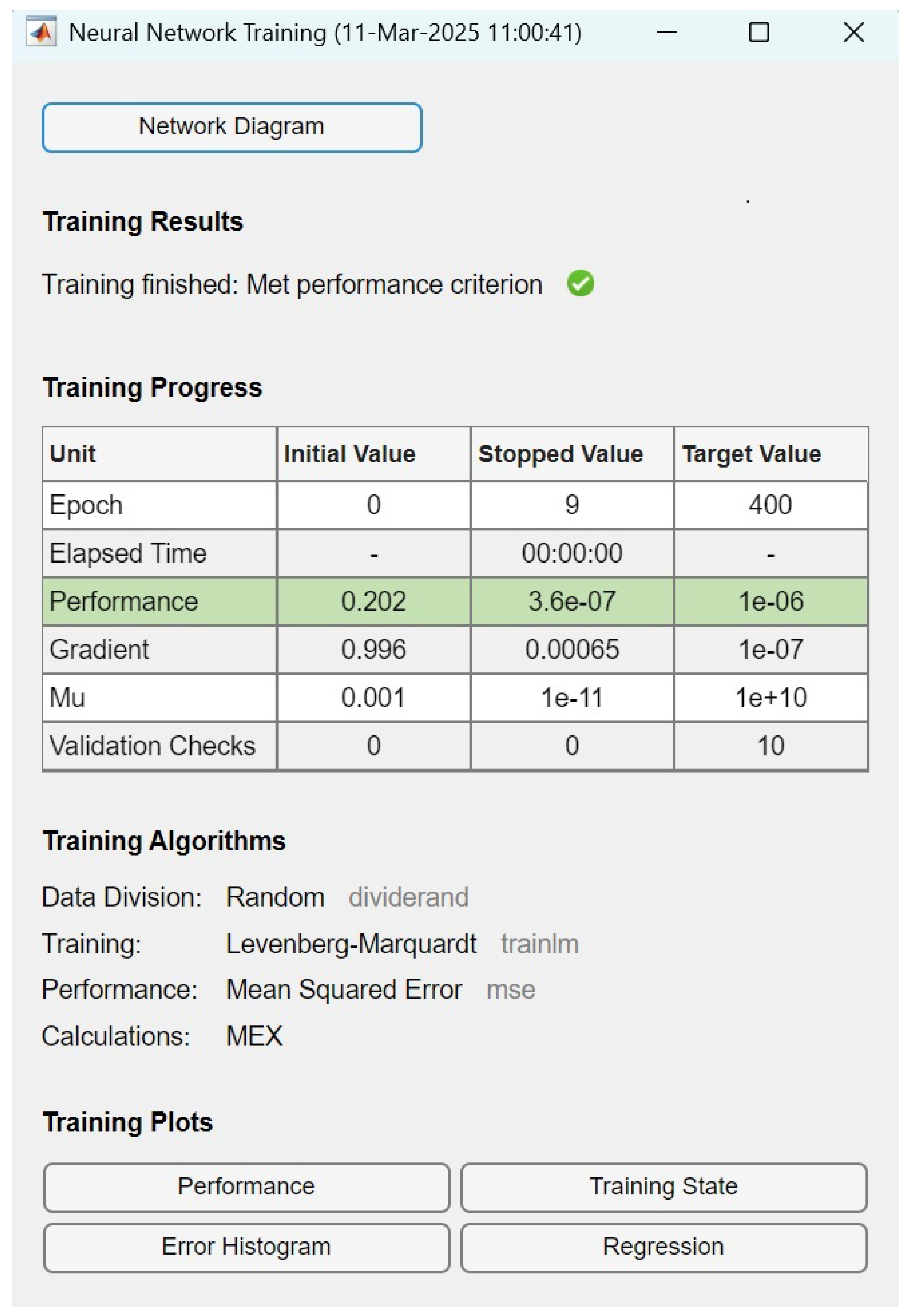
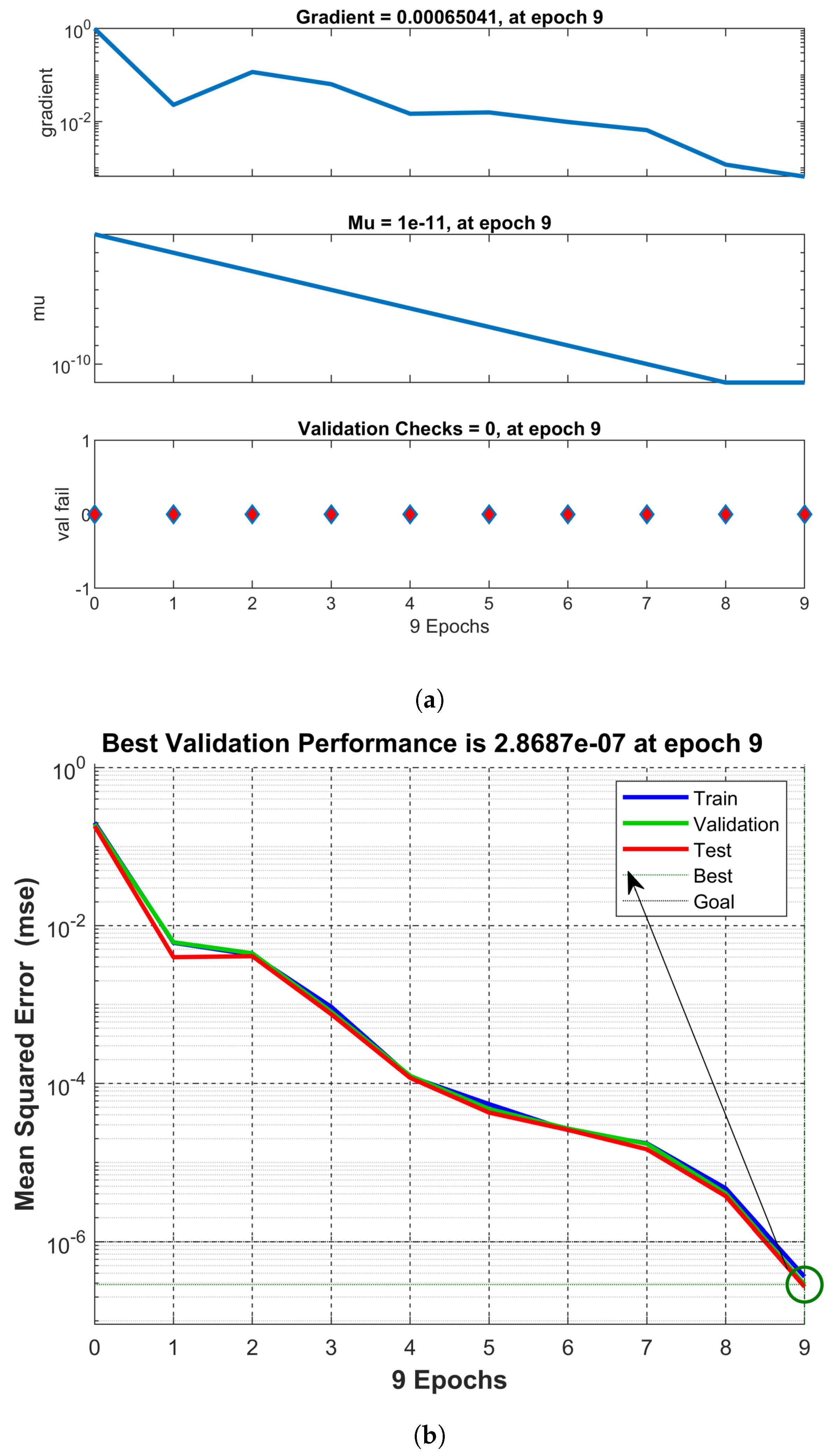
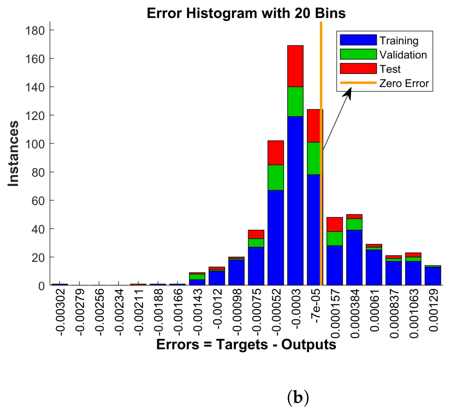
5. Deep Learning Analysis of Water Cycle Complex Neural Dynamical Mechanism

In this section, we explain how we trained an AI model to find an optimal function f that projects input data X to output Y and to minimize a loss function $L\left(f\right(X),Y)$ by adjusting model parameters for the water cycle using Complex Neural Dynamics. One of the best optimization algorithms in AI training is gradient descent, which enhances the parametric impacts iteratively:

$${\theta }^{(t+1)}={\theta }^{\left(t\right)}-{\eta }_0\nabla L\left({\theta }^{\left(t\right)}\right),$$

(10)

where $\theta$ represents model parameters (weights, biases) ${\eta }_0$ is the learning rate, and $\nabla L\left(\theta \right)$ is the gradient of the loss function. The use of the learning rate ${\eta }_0$ significantly impacts convergence. Too large a value yields instability, while too small a value results in slow convergence. In Figure 4a, the data are used to train a model for deep learning of the complex dynamics of the FF water cycle model (3) of order $0.98$.

A loss function measures the error between the predicted and actual values. The MSE is obtained by the relationship $MSE={\displaystyle \frac{1}{n}}{\sum }_{i=1}^n{({\mathcal{V}}_i-{\widehat{\mathcal{V}}}_i)}^2$, where ${\widehat{\mathcal{V}}}_i$ is the predicted output. Validation performance is assessed to determine how well the model generalizes to unseen data. The Cross-validation techniques were applied to ensure that the training data is effectively divided into training and validation classes. It was observed that the best validation performance of the technique was found at 759th epoch, and 1.1547 was obtained as the best result. At this value, the execution of simulations stopped.

5.1. Mean Square Error

This section is dedicated to the AI based analysis for mean square error of the computational data driven from the model (3). For this, 1330 points were considered. Among these data points, half were assumed for the input while half were targeted as output points. The data was trained as per Levenberg–Marquardt principles. The system targeted 400 epochs, but it reached the best validation in the early stage in only nine epochs, which confirms the accuracy of the data. The performance stopped at $3.6\times {10}^{-7}$, compared to a target of $1\times {10}^{-6}$. For the gradient, the initial value was taken as 0.996, and the simulations stopped at the value 0.00065 while it had a target of $1\times {10}^{-7}$. During this training, the data division was considered random. This can be observed in Figure 11 to Figure 12 in the deep learning results for the FF water cycle mechanism model (3) of order $0.98$ using Levenberg–Marquardt techniques for the performance, training state, error histogram, and regression estimations.

The best validation performance (BVF) was identified to be $2.8687\times {10}^{-7}$ at epoch 9, as given in Figure 12b. This refers to the minimum value of the mean square error (MSE) obtained during model validation where the

$$\mathrm{MSE}={\displaystyle \frac{1}{m}}\sum _{i=1}^m{({\mathcal{U}}_i-{\widehat{\mathcal{U}}}_i)}^2,$$

where ${\mathcal{U}}_i$ are actual values, ${\widehat{\mathcal{U}}}_i$ are predicted values, and m is the number of data points. A lower MSE shows better model accuracy. The BVF marks the optimal point where the model generalizes well to unseen data without overfitting or underfitting.

5.2. Regression of the Data

Regression models are used to predict continuous values corresponding to the input data points. We use linear and logistic regression for this analysis. The mathematical expression behind the linear regression is

$$Y={\vartheta }_0^{⊛}+{\vartheta }_1^{⊛}{\mathcal{U}}_1+{\vartheta }_2^{⊛}{\mathcal{U}}_2+\cdots +{\vartheta }_n^{⊛}{\mathcal{U}}_n+{ϵ}^{⊛},$$

(11)

where $ϵ⊛$ denotes the random error. The ${\vartheta }^{⊛}$ is produced by the following optimization procedure:

$$\widehat{{\vartheta }^{⊛}}={\left({\mathcal{U}}^T\mathcal{U}\right)}^{-1}{\mathcal{U}}^{T}Y$$

(12)

Logistic regression generates the probability of data and is based on the following relationship:

$$P(Y=1|\mathcal{U})={\displaystyle \frac{1}{1+e^{-({\vartheta }_0^{⊛}+{\vartheta }_1^{⊛}{\mathcal{U}}_1+\dots +{\vartheta }_n^{⊛}{\mathcal{U}}_n)}}}$$

(13)

This function, ensures output probabilities in between 0, to 1. An error histogram for the error distribution is computed as

$$E_i={}_m\mathcal{V}_i-m{\widehat{\mathcal{V}}}_i,$$

(14)

where, ${}_m\mathcal{V}_i$ are the actual values of the membrane potential while $m{\widehat{\mathcal{V}}}_i$ are the predicted values. One can see some more relevant works on the topic in [40]. We present regression analysis for training data where the output relation was considered as $1\times Target+1.1$, for the validation, the output data is evaluated by the expression $1\times Target+1.1$, the same relation was assumed for the testing data sets as well. In all these cases we observed R = 1. Which affirm the best performance of the technique in our works. It is described in Figure 13a. The error histogram was also analyzed, and most of the data were surrounded by the zero error line given in Figure 13b. This error was evaluated by the relationship $Error=Targets-Outputs$.

6. Conclusions

In this article, we considered an FF water cycle mathematical model (3) with three variables; $\mathfrak{T}$ represents the global temperature, $\mathcal{P}$ represents the precipitation of atmospheric water, and $\mathcal{W}$ represents the water availability. There are several parameters that correlate with the variables; these parameters are expressed in Table 1. The model is first mathematically analyzed for the existence and stability of a solution subject to the assumptions $\left(\mathcal{A}\right)$ and $\left(\mathcal{B}\right)$. The model was computationally solved by a numerical scheme, and the results were illustrated in multiple figures. The impact of the parameters was analyzed to identify their role in the time course of the global temperature, the degree of uncertainty in the ecosystem, and the occurrence of catastrophic runoff. These results were tested by AI techniques for the error and regression of the data points, and the regression revealed a correlation coefficient equal to one on the training, validation, and test data. An error analysis and the best performance results were also obtained, and the corresponding epochs were calculated. This integrated system of mathematical modeling with AI can further be utilized on real data sets for deeper insights into the environmental factors influencing the ecosystems of the planet.

References

1. Trenberth, K.E. Water cycles and climate change. Glob. Environ. Chang. 2014, 2014, 31–37. [Google Scholar]
2. Yang, K.; Wu, H.; Qin, J.; Lin, C.; Tang, W.; Chen, Y. Recent climate changes over the Tibetan Plateau and their impacts on energy and water cycle: A review. Glob. Planet. Chang. 2014, 112, 79–91. [Google Scholar] [CrossRef]
3. Wu, Y.; Liu, S.; Gallant, A.L. Predicting impacts of increased CO2 and climate change on the water cycle and water quality in the semiarid James River Basin of the Midwestern USA. Sci. Total Environ. 2012, 430, 150–160. [Google Scholar] [CrossRef]
4. Nan, Y.; Men, B.; Lin, C.-K. Impact analysis of climate change on water resources. Procedia Eng. 2011, 24, 643–648. [Google Scholar] [CrossRef]
5. Barry, S.M.; Davies, G.R.; Forton, J.; Williams, S.; Thomas, R.; Paxton, P.; Moore, G.; Davies, C.R. Trends in low global warming potential inhaler prescribing: A UK-wide cohort comparison from 2018–2024. NPJ Prim. Care Respir. Med. 2025, 35, 9. [Google Scholar] [CrossRef] [PubMed]
6. An, R.; Ji, M.; Zhang, S. Global warming and obesity: A systematic review. Obes. Rev. 2018, 19, 150–163. [Google Scholar] [CrossRef]
7. Cao, M.; Wang, F.; Ma, S.; Geng, H.; Sun, K. Recent advances on greenhouse gas emissions from wetlands: Mechanism, global warming potential, and environmental drivers. Environ. Pollut. 2024, 355, 124204. [Google Scholar] [CrossRef]
8. Amnuaylojaroen, T. Perspective on the era of global boiling: A future beyond global warming. Adv. Meteorol. 2023, 2023, 5580606. [Google Scholar] [CrossRef]
9. Janni, M.; Maestri, E.; Gullì, M.; Marmiroli, M.; Marmiroli, N. Plant responses to climate change, how global warming may impact on food security: A critical review. Front. Plant Sci. 2024, 14, 1297569. [Google Scholar] [CrossRef]
10. Ripple, W.J.; Wolf, C.; Gregg, J.W.; Rockström, J.; Mann, M.E.; Oreskes, N.; Lenton, T.M.; Rahmstorf, S.; Newsome, T.M.; Xu, C.; et al. The 2024 state of the climate report: Perilous times on planet Earth. BioScience 2024, 74, 812–824. [Google Scholar] [CrossRef]
11. Van Daalen, K.R.; Tonne, C.; Semenza, J.C.; Rocklöv, J.; Markandya, A.; Dasandi, N.; Jankin, S.; Achebak, H.; Ballester, J.; Bechara, H.; et al. The 2024 Europe report of the Lancet Countdown on health and climate change: Unprecedented warming demands unprecedented action. Lancet Public Health 2024, 9, e495–e522. [Google Scholar] [CrossRef] [PubMed]
12. Cai, W.; Zhang, C.; Zhang, S.; Bai, Y.; Callaghan, M.; Chang, N.; Chen, B.; Chen, H.; Cheng, L.; Dai, H.; et al. The 2024 China report of the Lancet Countdown on health and climate change: Launching a new low-carbon, healthy journey. Lancet Public Health 2024, 9, e1070–e1088. [Google Scholar] [CrossRef]
13. Su, Y.; Ullah, K. Exploring the correlation between rising temperature and household electricity consumption: An empirical analysis in China. Heliyon 2024, 10, e30130. [Google Scholar] [CrossRef] [PubMed]
14. Yaseen, R.M.; Ali, N.F.; Mohsen, A.A.; Khan, A.; Abdeljawad, T. The modeling and mathematical analysis of the fractional-order of Cholera disease: Dynamical and Simulation. Partial Differ. Equ. Appl. Math. 2024, 12, 100978. [Google Scholar] [CrossRef]
15. Alsaadi, A. Advancing water quality management: A synergistic approach using fractional differential equations and neural networks. AIMS Math. 2025, 10, 5332–5352. [Google Scholar] [CrossRef]
16. Bedi, P.; Kumar, A.; Deora, G.; Khan, A.; Abdeljawad, T. An investigation into the controllability of multivalued stochastic fractional differential inclusions. Chaos Solitons Fractals X 2024, 12, 100107. [Google Scholar] [CrossRef]
17. Nordhaus, W.D.; Boyer, J. Warming the World: Economic Models of Global Warming; MIT Press: Cambridge, MA, USA, 2003. [Google Scholar]
18. Nobre, P.; Malagutti, M.; Urbano, D.F.; de Almeida, R.A.; Giarolla, E. Amazon deforestation and climate change in a coupled model simulation. J. Climate 2009, 22, 5686–5697. [Google Scholar] [CrossRef]
19. Henderson-Sellers, A.; Dickinson, R.E.; Wilson, M.F. Tropical deforestation: Important processes for climate models. Clim. Chang. 1988, 13, 43–67. [Google Scholar] [CrossRef]
20. Sabatier, J.A.; Agrawal, O.P.; Machado, J.T. Advances in Fractional Calculus; Springer: Dordrecht, The Netherlands, 2007. [Google Scholar]
21. Herrmann, R. Fractional Calculus: An Introduction for Physicists; World Scientific: Singapore, 2011. [Google Scholar]
22. Caputo, M.; Fabrizio, M. A new definition of fractional derivative without singular kernel. Prog. Fract. Differ. Appl. 2015, 1, 73–85. [Google Scholar]
23. Bas, E.; Acay, B.; Ozarslan, R. Fractional models with singular and non-singular kernels for energy efficient buildings. Chaos 2019, 29, 023110. [Google Scholar] [CrossRef]
24. Khan, A.; Abdeljawad, T.; Abdel-Aty, M.; Almutairi, D.K. Digital analysis of discrete fractional order cancer model by artificial intelligence. Alex. Eng. J. 2025, 118, 115–124. [Google Scholar] [CrossRef]
25. Khan, A.; Abdeljawad, T.; Alkhawar, H.M. Digital analysis of discrete fractional order worms transmission in wireless sensor systems: Performance validation by artificial intelligence. Model. Earth Syst. Environ. 2025, 11, 25. [Google Scholar] [CrossRef]
26. Ahmad, I.; Bakar, A.A.; Ahmad, H.; Khan, A.; Abdeljawad, T. Investigating virus spread analysis in computer networks with Atangana–Baleanu fractional derivative models. Fractals 2024, 2440043, 17. [Google Scholar] [CrossRef]
27. Atangana, A. Fractal–fractional differentiation and integration: Connecting fractal calculus and fractional calculus to predict complex system. Chaos Solitons Fractals 2017, 102, 396–406. [Google Scholar] [CrossRef]
28. Atangana, A.; Qureshi, S. Modeling attractors of chaotic dynamical systems with fractal–fractional operators. Chaos Solitons Fractals 2019, 123, 320–337. [Google Scholar] [CrossRef]
29. Atangana, A.; Araz, S.I. Atangana–Seda numerical scheme for Labyrinth attractor with new differential and integral operators. Fractals 2020, 28, 2040044. [Google Scholar] [CrossRef]
30. Sekerci, Y. Climate change effects on fractional order prey-predator model. Chaos Solitons Fractals 2020, 134, 109690. [Google Scholar] [CrossRef]
31. Khan, H.; Aslam, M.; Rajpar, A.H.; Chu, Y.M.; Etemad, S.; Rezapour, S.; Ahmad, H. A new fractal-fractional hybrid model for studying climate change on coastal ecosystems from the mathematical point of view. Fractals. 2024, 32, 2440015. [Google Scholar] [CrossRef]
32. Kumar, P.; Erturk, V.S.; Banerjee, R.; Yavuz, M.; Govindaraj, V. Fractional modeling of plankton-oxygen dynamics under climate change by the application of a recent numerical algorithm. Phys. Scr. 2021, 96, 124044. [Google Scholar] [CrossRef]
33. Kumar, V.R.; Mani, N. The application of artificial intelligence techniques for intelligent control of dynamical physical systems. Int. J. Adapt. Control Signal Process. 1994, 8, 379–392. [Google Scholar] [CrossRef]
34. Böttcher, L.; Antulov-Fantulin, N.; Asikis, T. AI Pontryagin or how artificial neural networks learn to control dynamical systems. Nat. Commun. 2022, 13, 333. [Google Scholar] [CrossRef] [PubMed]
35. Yuksel, G. Dynamical Systems and Artificial Intelligence. In Artificial Intelligence; CRC Press: Boca Raton, FL, USA, 2024; pp. 75–83. [Google Scholar]
36. Sharma, P.; Khan, J.S.; Radhika, K.; Thatipudi, J.G.; Sridevi, K.; Upadhyay, S. Evolutionary Intelligence: A Hybrid Neural Framework for Dynamic System Innovation. In Proceedings of the 2025 International Conference on Electronics and Renewable Systems (ICEARS), Thoothukudi, India, 1–13 February 2025; pp. 1743–1749. [Google Scholar]
37. Khan, H.; Alzabut, J.; Almutairi, D.K.; Alqurashi, W.K. The Use of Artificial Intelligence in Data Analysis with Error Recognitions in Liver Transplantation in HIV-AIDS Patients Using Modified ABC Fractional Order Operators. Fractal Fract. 2025, 9, 16. [Google Scholar] [CrossRef]
38. Khan, H.; Alzabut, J.; Tounsi, M.; Almutairi, D.K. AI-Based Data Analysis of Contaminant Transportation with Regression of Oxygen and Nutrients Measurement. Fractal Fract. 2025, 9, 125. [Google Scholar] [CrossRef]
39. Khan, A.; Shah, K.; Abdeljawad, T.; Alqudah, M.A. Existence of results and computational analysis of a fractional order two strain epidemic model. Results Phys. 2022, 39, 105649. [Google Scholar] [CrossRef]
40. Wan-Arfah, N.; Muzaimi, M.; Naing, N.N.; Subramaniyan, V.; Wong, L.S.; Selvaraj, S. Prognostic factors of first-ever stroke patients in suburban Malaysia by comparing regression models. Electron. J. Gen. Med. 2023, 20, em545. [Google Scholar] [CrossRef]
Figure 1. The water cycle, comprising evaporation and precipitation (rainfall).
Fractalfract 09 00361 g001
Figure 2. Diagrammatic structure of the water cycle mechanism given by model (3).
Fractalfract 09 00361 g002
Figure 3. Temperature variation estimation for the next 80 years under the effects of A = 0.01 , 0.02 , 0.03 , 0.04 and B = 0.0025 , 0.005 , 0.0075 , 0.01 for FF order 0.98 . (a) Temperature variation estimation for the next 80 years under the effects of A = 0.01 , 0.02 , 0.03 , 0.04 for FF order 0.98 . (b) Temperature variation estimation for the next 80 years under the effects of B = 0.0025 , 0.005 , 0.0075 , 0.01 for FF order 0.98 .
Fractalfract 09 00361 g003
Figure 4. Temperature variation estimation for the next 80 years under the effects of E = 0.0025 , 0.005 , 0.0075 , 0.01 and η = 0.0025 , 0.005 , 0.0075 , 0.01 for FF water cycle model (3) of order 0.98 . (a) Temperature variation estimation for the next 80 years under the effects of E = 0.0025 , 0.005 , 0.0075 , 0.01 for FF order 0.98 . (b) Temperature variation estimation for the next 80 years under the effects of η = 0.0025 , 0.005 , 0.0075 , 0.01 for fixed FF order 0.98 .
Fractalfract 09 00361 g004
Figure 5. Temperature and water level estimation for the next 80 years under the effects of T e q = 285 , 288 , 291 , 294 and E = 0.0025 , 0.005 , 0.0075 , 0.01 for FF water cycle model (3) of order 0.98 . (a) Temperature variation estimation for the next 80 years under the effects of T e q = 285 , 288 , 291 , 294 for FF water cycle model (3) of order 0.98 . (b) Water level estimation for the next 80 years under the effects of E = 0.0025 , 0.005 , 0.0075 , 0.01 for FF water cycle model (3) of order 0.98 .
Fractalfract 09 00361 g005
Figure 6. Water level estimation for the next 80 years under the variation of the runoff factor F , η = 0.0025 , 0.005 , 0.0075 , 0.01 for FF water cycle model (3) of order 0.98 . (a) Water level estimation for the next 80 years under the variation of the runoff factor F = 0.0025 , 0.005 , 0.0075 , 0.01 for FF water cycle model (3) of order 0.98 . (b) Water level estimation for the next 80 years under the variation of the runoff factor η = 0.0025 , 0.005 , 0.0075 , 0.01 for FF water cycle model (3) of order 0.98 .
Fractalfract 09 00361 g006
Figure 7. The impact of T e q = 285 , 288 , 291 , 294 and θ = 0.0025 , 0.005 , 0.0075 , 0.01 on the water level for the next 80 years as per FF water cycle model (3) of order 0.98 . (a) The impact of T e q = 285 , 288 , 291 , 294 on the water level for the next 80 years as per FF water cycle model (3) of order 0.98 . (b) The estimated impact of θ = 0.0025 , 0.005 , 0.0075 , 0.01 on the water level for the next 80 years for FF water cycle model (3) of order 0.98 .
Fractalfract 09 00361 g007
Figure 8. The estimated impact of E , η = 0.0025 , 0.005 , 0.0075 , 0.01 on the water precipitation for the next 80 years as per FF water cycle model (3) of order 0.98 . (a) The estimated impact of E = 0.0025 , 0.005 , 0.0075 , 0.01 on water precipitation for the next 80 years. (b) The estimated impact of η = 0.0025 , 0.005 , 0.0075 , 0.01 on water precipitation for the next 80 years.
Fractalfract 09 00361 g008
Figure 9. The estimated impact of E , η = 0.0025 , 0.005 , 0.0075 , 0.01 on water precipitation for the next 80 years as per FF water cycle model (3) of order 0.98 . (a) The estimated impact of E = 0.0025 , 0.005 , 0.0075 , 0.01 on water precipitation for the next 80 years. (b) The estimated impact of η = 0.0025 , 0.005 , 0.0075 , 0.01 on water precipitation for the next 80 years.
Fractalfract 09 00361 g009
Figure 10. The estimated impact of λ = 0.0005 , 0.001 , 0.0015 , 0.002 on water precipitation for the next 80 years as per FF water cycle model (3) of order 0.98 .
Fractalfract 09 00361 g010
Figure 11. Deep Learning results for the FF water cycle mechanism model (3) of order 0.98 by Levenberg–Marquardt techniques for the performance, training state, error histogram, and regression estimations.
Fractalfract 09 00361 g011
Figure 12. Training the models data for the deep learning-based analysis of water cycle mechanism model (3) and best validation performance 2.8687 × 10 7 at 9th epoch. (a) Training of the data for the deep learning of complex FF water cycle system model (3) of order 0.98 . (b) Mean Square Error for the complex dynamics of FF water cycle mechanism model (3) of order 0.98 .
Fractalfract 09 00361 g012
Figure 13. Deep learning results for water cycle mechanism (3) for the FF orders 0.98 by Levenberg–Marquardt techniques for regression and error estimations. (a) Regression analysis in the training, validation and test data sets for the water cycle mechanism. (b) Error histogram to highlight the training, validation, test data with the zero error in the water cycle mechanism.
Fractalfract 09 00361 g013aFractalfract 09 00361 g013b