An Efficient Structure-Preserving Scheme for the Fractional Damped Nonlinear Schrödinger System

Abstract

This paper introduces a highly accurate and efficient conservative scheme for solving the nonlocal damped Schrödinger system with Riesz fractional derivatives. The proposed approach combines the Fourier spectral method with the Crank–Nicolson time-stepping scheme. To begin, the original equation is reformulated into an equivalent system by introducing a new variable that modifies both energy and mass. The Fourier spectral method is employed to achieve high spatial accuracy in this semi-discrete formulation. For time discretization, the Crank–Nicolson scheme is applied, ensuring conservation of the modified energy and mass in the fully discrete system. Numerical experiments validate the scheme’s precision and its ability to preserve conservation properties.

1. Introduction

The Riesz space fractional nonlinear Schrödinger equation, widely recognized for its capacity to model long-range interactions via fractional-order derivatives, has become a key framework for studying complex phenomena in quantum mechanics, condensed matter physics, plasma physics, nonlinear optics, wave propagation dynamics, and fluid dynamics, etc. [1,2,3,4,5]. However, in many physical systems, energy dissipation or damping play a crucial role. Damping, often resulting from interactions with the external environment, is key to accurately capturing the dynamics of these systems, especially in cases involving wave propagation, energy loss, and long-term stabilization. Introducing a damping term into the fractional nonlinear Schrödinger equation yields the damped fractional nonlinear Schrödinger (DFNLS) equation

$$\mathrm{i}{\mathsf{\partial }}_t\psi -{\left(-\Delta \right)}^{{\displaystyle \frac{\alpha }{2}}}\psi +\beta {\left|\psi \right|}^2\psi +\mathrm{i}\omega \psi =0,x\in (-L,L),0<t⩽T,$$

(1)

with the initial condition

$$\psi (x,0)={\psi }_0\left(x\right),x\in (-L,L),$$

(2)

and the periodic boundary condition

$$\psi (-L,t)=\psi (L,t),0<t⩽T,$$

(3)

where $\mathrm{i}=\sqrt{-1}$ and $1<\alpha \le 2$. Here, $\psi (x,t)$ is a complex-valued wave function, $\beta$ is a real constant representing the strength of interactions between nearby particles, and $\omega$ is a non-negative damping coefficient characterizing dissipation. The function ${\psi }_0\left(x\right)$ is a given smooth complex-valued function. The fractional Laplacian $-{(-\Delta )}^{{\displaystyle \frac{\alpha }{2}}}$ acting on a periodic function is defined in [6] as

$$-{\left(-\Delta \right)}^{{\displaystyle \frac{\alpha }{2}}}\psi \left(x,t\right)=-\sum _{k\in \mathbb{Z}}{\left|v_k\right|}^{\alpha }{\widehat{\psi }}_k{\mathrm{e}}^{\mathrm{i}{v}_k(x+L)},$$

where $v_k=k\pi /L$ and the Fourier coefficient ${\widehat{\psi }}_k$ is defined by

$${\widehat{\psi }}_k={\displaystyle \frac{1}{2L}}{\int }_{-L}^L\psi (x,t){\mathrm{e}}^{-\mathrm{i}{v}_k(x+L)}\mathrm{d}x.$$

When $\alpha =2$, the fractional Laplacian reduces to the classical integer-order Laplace operator, and the DFNLS equation simplifies to the standard damped nonlinear Schrödinger equation. This classical equation, describing certain resonance phenomena in nonlinear media, has been extensively studied by both physicists and mathematicians [7,8,9,10,11].

In recent decades, the DFNLS equation has garnered significant interest within the mathematical community. Tarek [12] explored the global existence and scattering properties of solutions for a semi-linear fractional damped Schrödinger equation, highlighting the impact of the damping coefficient. Liang et al. [13] established the unique existence of global smooth solutions for the DFNLS equation. The DFNLS equation poses significant mathematical challenges, due to the complex interaction between nonlocal fractional operators and damping effects, which makes analytical solutions particularly difficult to obtain. Consequently, numerical methods are essential for investigating this equation, as they enable researchers to examine how damping influences soliton formation, wave decay, and other dynamic behaviors in intricate systems. Recently, various innovative numerical schemes have been developed to solve the DFNLS equation. For instance, in Ref. [13], a conformal mass-preserving linearized scheme was introduced, with a rigorous proof of its second-order spatial accuracy and first-order temporal accuracy, along with the preservation of discrete conformal mass. Fu et al. [14] proposed a numerical scheme for the DFNLS equation, offering a novel error estimate in the maximum norm and demonstrating second-order accuracy in both time and space. Wu et al. [15] examined conservation laws and the convergence of a splitting conformal multisymplectic scheme for the two-dimensional DFNLS equation, showing second-order accuracy in time, spectral accuracy in space, and validating these results with numerical experiments. Ding et al. [16] proposed a novel high-order structure-preserving scheme for the DFNLS equation, achieving fourth-order accuracy in space, while conserving mass and energy, with a detailed analysis on boundedness, uniqueness, and convergence, supported by extensive numerical results. The Fourier spectral method is particularly effective for problems involving fractional derivatives defined via Fourier decomposition, thanks to the diagonal structure of the operator, which enables efficient solvers. The application of Fourier spectral methods to the classical fractional Schrödinger equation has been explored in recent literature [17,18,19,20], offering important insights and a foundation for the development of accurate and efficient numerical approaches in this area. However, to the best of our knowledge, there have been no publications that utilized spectral methods to solve the DFNLS equation and provide a detailed theoretical analysis.

The main contributions of this paper are as follows:

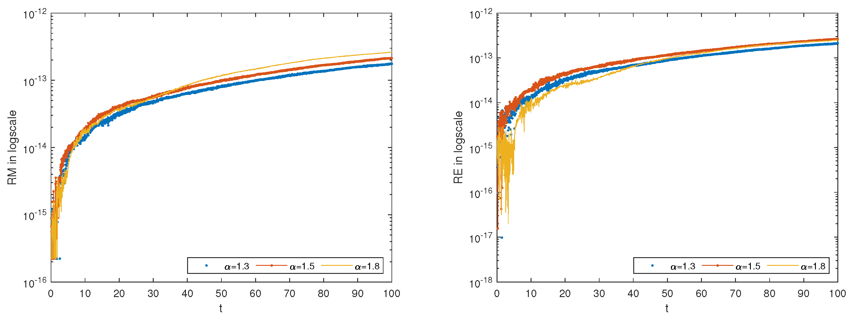
• An exponential variable is introduced to derive an equivalent formulation of the DFNLS equation, accompanied by a rigorous proof of the conservation of two quantities in this form.
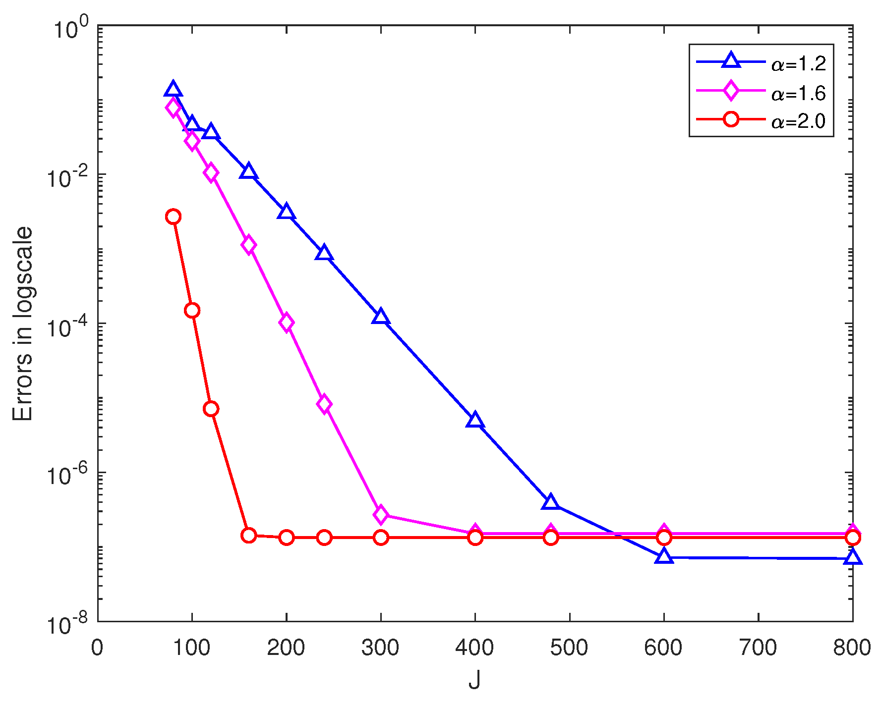
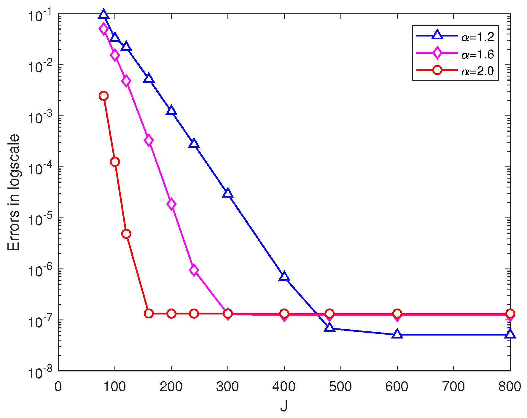
• A semi-discrete scheme utilizing the Fourier spectral method in space is proposed, demonstrating its conservation properties and spectral accuracy convergence.
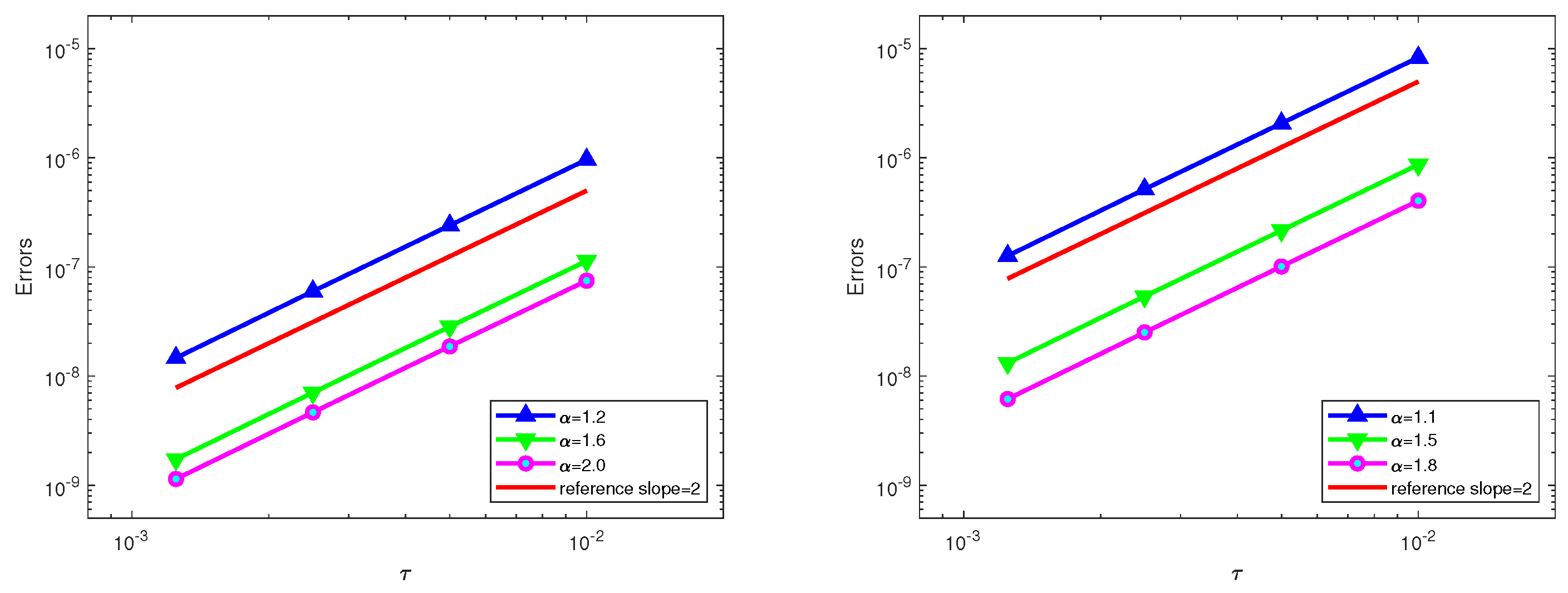
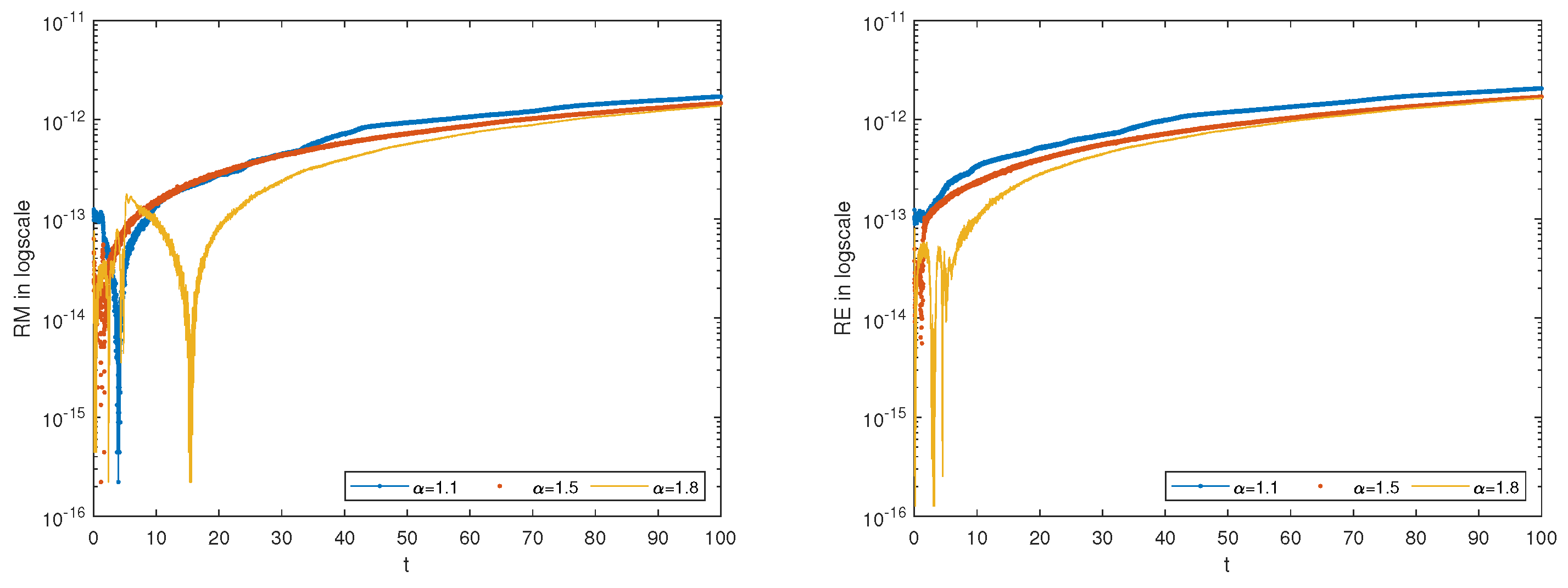
• A fully-discrete scheme is developed by integrating the Fourier spectral method in space with the Crank–Nicolson method in time, establishing its conservation and convergence properties.
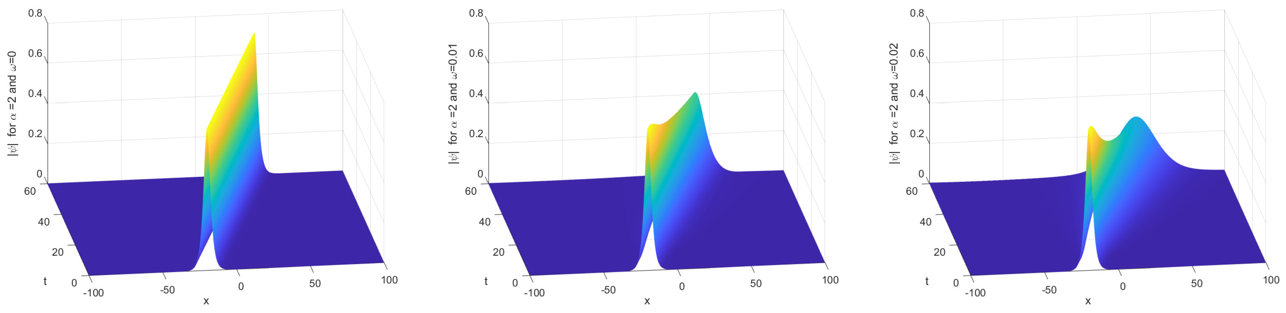
• The theoretical findings are validated through numerical experiments, which also confirm the method’s effectiveness in addressing fractional high-dimensional problems.

The remainder of this paper is organized as follows: Section 2 introduces an exponential variable to derive an equivalent system featuring two conserved quantities. Section 3 develops a semi-discrete scheme utilizing the Fourier spectral method, which preserves both energy and mass. In Section 4, the Crank–Nicolson method is applied to the semi-discrete system, resulting in a fully conservative scheme. Section 5 presents numerical results that validate the theoretical analysis, while Section 6 concludes by summarizing the main findings.

2. Reformulated System

To develop a structure-preserving numerical algorithm, we adopt a method similar to the Lawson transform [21]. Specifically, we define

$$u(x,t)={\mathrm{e}}^{\omega t}\psi (x,t).$$

(4)

This allows us to further reduce the DFNLS system (1)–(3) to the following modified DFNLS (M-DFNLS) system:

$$\begin{array}{cc}\hfill & \mathrm{i}{\mathsf{\partial }}_{t}u-{(-\Delta )}^{{\displaystyle \frac{\alpha }{2}}}u+\beta {\mathrm{e}}^{-2\omega t}{\left|u\right|}^{2}u=0,x\in (-L,L),0<t⩽T,\hfill \end{array}$$

(5)

$$\begin{array}{cc}\hfill & u(x,0)={\psi }_0\left(x\right),x\in (-L,L),\hfill \end{array}$$

(6)

$$\begin{array}{cc}\hfill & u(-L,t)=u(L,t),0<t⩽T.\hfill \end{array}$$

(7)

For simplicity, we denote $\Omega =[-L,L]$ and assume that $L^2(\Omega )$ consists of square-integrable Lebesgue functions over $\Omega$. We then define the following inner product and norms:

$$\begin{array}{c}{\left(u,v\right)}_{L^2}={\int }_{\Omega }u\overline{v}\mathrm{d}x,{\parallel u\parallel }^2={\left(u,u\right)}_{L^2}\\ {\parallel u\parallel }_{L^p}^p={\int }_{\Omega }{\left|u\right|}^p\mathrm{d}x,1\le p\le +{\infty ,\parallel u\parallel }_{\infty }=\mathrm{ess}\underset{x\in \Omega }{sup}\left|u\left(x\right)\right|.\end{array}$$

By leveraging certain properties of the fractional Laplacian operator, we can readily demonstrate that the system (5)–(7) satisfies the conservation laws for mass and energy.

Theorem 1.

If $u(x,t)$ is the solution to the M-DFNLS system (5)–(7), then the system exhibits the following conservation laws for mass and energy:

$$\mathcal{M}\left(t\right)\equiv \mathcal{M}\left(0\right),\mathcal{E}\left(t\right)\equiv \mathcal{E}\left(0\right),t>0,$$

where

$$\begin{array}{cc}\hfill & \mathcal{M}\left(t\right)={\int }_{\Omega }{\left|u(x,t)\right|}^2\mathrm{d}x,\hfill \\ \hfill & \mathcal{E}\left(t\right)={\int }_{\Omega }\left[{|(-\Delta )}^{{\displaystyle \frac{\alpha }{4}}}{u(x,t)|}^2-{\displaystyle \frac{\beta }{2}}{\mathrm{e}}^{-2\omega t}{\left|u(x,t)\right|}^4\right]\mathrm{d}x-\omega \beta {\int }_0^t{\mathrm{e}}^{-2\omega s}{\int }_{\Omega }{\left|u(x,s)\right|}^4\mathrm{d}x\mathrm{d}s.\hfill \end{array}$$

Proof. 

Based on the proof proposed by [22], for any periodic complex-valued functions u and v, we have

$${\int }_{\Omega }\left({(-\Delta )}^{{\displaystyle \frac{\alpha }{2}}}u\right)\overline{v}\mathrm{d}x={\int }_{\Omega }\left({(-\Delta )}^{{\displaystyle \frac{\alpha }{4}}}u\right)\left({(-\Delta )}^{{\displaystyle \frac{\alpha }{4}}}\overline{v}\right)\mathrm{d}x.$$

(8)

Then, according to the chain rule and Equation (8), we can verify the mass conservation law by a direct calculation

$$\begin{array}{cc}\hfill {\displaystyle \frac{\mathrm{d}}{\mathrm{d}t}}\mathcal{M}\left(t\right)& ={\int }_{\Omega }\left[\left({\mathsf{\partial }}_{t}u\right)\overline{u}+u\left({\mathsf{\partial }}_t\overline{u}\right)\right]\mathrm{d}x\hfill \\ \hfill & ={\int }_{\Omega }\left[\left(-\mathrm{i}{\left(-\Delta \right)}^{{\displaystyle \frac{\alpha }{2}}}u+\mathrm{i}\beta {\mathrm{e}}^{-2\omega t}{\left|u\right|}^{2}u\right)\overline{u}+u\left(\mathrm{i}{\left(-\Delta \right)}^{{\displaystyle \frac{\alpha }{2}}}\overline{u}-\mathrm{i}\beta {\mathrm{e}}^{-2\omega t}{\left|u\right|}^2\overline{u}\right)\right]\mathrm{d}x\hfill \\ \hfill & ={\int }_{\Omega }\left[-\mathrm{i}{\left(-\Delta \right)}^{{\displaystyle \frac{\alpha }{2}}}u\overline{u}+\mathrm{i}u{\left(-\Delta \right)}^{{\displaystyle \frac{\alpha }{2}}}\overline{u}\right]\mathrm{d}x\hfill \\ \hfill & ={\int }_{\Omega }\left[-\mathrm{i}\left({\left(-\Delta \right)}^{{\displaystyle \frac{\alpha }{4}}}u\right)\left({\left(-\Delta \right)}^{{\displaystyle \frac{\alpha }{4}}}\overline{u}\right)+\mathrm{i}\left({\left(-\Delta \right)}^{{\displaystyle \frac{\alpha }{4}}}u\right)\left({\left(-\Delta \right)}^{{\displaystyle \frac{\alpha }{4}}}\overline{u}\right)\right]\mathrm{d}x\hfill \\ \hfill & =0.\hfill \end{array}$$

Next, we can similarly derive the energy conservation law, as follows:

$$\begin{array}{cc}\hfill {\displaystyle \frac{\mathrm{d}}{\mathrm{d}t}}\mathcal{E}\left(t\right)=& {\int }_{\Omega }\left[\left({\left(-\Delta \right)}^{{\displaystyle \frac{\alpha }{4}}}{\mathsf{\partial }}_{t}u\right)\left({\left(-\Delta \right)}^{{\displaystyle \frac{\alpha }{4}}}\overline{u}\right)+\left({\left(-\Delta \right)}^{{\displaystyle \frac{\alpha }{4}}}u\right)\left({\left(-\Delta \right)}^{{\displaystyle \frac{\alpha }{4}}}{\mathsf{\partial }}_t\overline{u}\right)\right]\mathrm{d}x+\beta \omega {\mathrm{e}}^{-2\omega t}{\int }_{\Omega }{\left|u\right|}^4\mathrm{d}x\hfill \\ \hfill & -{\displaystyle \frac{\beta }{2}}{\mathrm{e}}^{-2\omega t}{\int }_{\Omega }[\left({\mathsf{\partial }}_{t}u\right){\left|u\right|}^2\overline{u}+{\left|u\right|}^2\left({\mathsf{\partial }}_{t}u\right)\overline{u}+u\left({\mathsf{\partial }}_t\overline{u}\right){\left|u\right|}^2+{\left|u\right|}^{2}u\left({\mathsf{\partial }}_t\overline{u}\right)]\mathrm{d}x-\omega \beta {\mathrm{e}}^{-2\omega t}{\int }_{\Omega }{\left|u\right|}^4\mathrm{d}x\hfill \\ \hfill =& {\int }_{\Omega }\left[\left({\mathsf{\partial }}_{t}u\right)\left({\left(-\Delta \right)}^{{\displaystyle \frac{\alpha }{2}}}\overline{u}\right)+\left({\left(-\Delta \right)}^{{\displaystyle \frac{\alpha }{2}}}u\right)\left({\mathsf{\partial }}_t\overline{u}\right)\right]\mathrm{d}x-\beta {\mathrm{e}}^{-2\omega t}{\int }_{\Omega }\left[\left({\mathsf{\partial }}_{t}u\right){\left|u\right|}^2\overline{u}+{\left|u\right|}^{2}u\left({\mathsf{\partial }}_t\overline{u}\right)\right]\mathrm{d}x\hfill \\ \hfill =& {\int }_{\Omega }\left[\left({\mathsf{\partial }}_{t}u\right)\left({\left(-\Delta \right)}^{{\displaystyle \frac{\alpha }{2}}}\overline{u}-\beta {\mathrm{e}}^{-2\omega t}{\left|u\right|}^2\overline{u}\right)+\left({\left(-\Delta \right)}^{{\displaystyle \frac{\alpha }{2}}}u-\beta {\mathrm{e}}^{-2\omega t}{\left|u\right|}^{2}u\right)\left({\mathsf{\partial }}_t\overline{u}\right)\right]\mathrm{d}x\hfill \\ \hfill =& {\int }_{\Omega }\left[\left({\mathsf{\partial }}_{t}u\right)\left(-\mathrm{i}{\mathsf{\partial }}_t\overline{u}\right)+\left(\mathrm{i}{\mathsf{\partial }}_{t}u\right)\left({\mathsf{\partial }}_t\overline{u}\right)\right]\mathrm{d}x\hfill \\ \hfill =& 0.\hfill \end{array}$$

This completes the proof. □

3. Construction of Semi-Discrete Fourier Spectral Scheme and Theoretical Analysis

3.1. Some Useful Lemmas

For any real number $r>0$, let

$$H^r\left(\Omega \right)=\left\{u\right|u\in L^2\left(\Omega \right),D^{k}u\in L^2\left(\Omega \right),\forall \left|k\right|\le r\},$$

be a Sobolev space with norm $\parallel ·\parallel$ and semi-norm $|·|$. Denote $H_{\mathrm{per}}^r\left(\Omega \right)$ as a subspace composed of functions with $2L$-period in $H^r\left(\Omega \right)$, i.e.,

$$H_{\mathrm{per}}^r\left(\Omega \right)=\left\{u\right|u\in H^r\left(\Omega \right),u\left(x-L\right)=u\left(x+L\right)\},$$

and the norm and semi-norm are

$${\parallel u\parallel }_r={\left(\sum _{k=-\infty }^{\infty }{\left(1+{\left|k\right|}^2\right)}^r{\left|{\widehat{u}}_k\right|}^2\right)}^{1/2},{\left|u\right|}_r={\left(\sum _{k=-\infty }^{\infty }{\left|k\right|}^{2r}{\left|{\widehat{u}}_k\right|}^2\right)}^{1/2},$$

where

$$u\left(x\right)=\sum _{k=-\infty }^{\infty }{\widehat{u}}_k{\mathrm{e}}^{\mathrm{i}k(x+L)},{\widehat{u}}_k={\displaystyle \frac{1}{2\pi }}{\int }_{\Omega }u\left(x\right){\mathrm{e}}^{-\mathrm{i}k(x+L)}\mathrm{d}x.$$

Let

$$C([0,T];X)=\{u(·,t)\in X:\underset{0\le t\le T}{sup}\parallel u(·,t){\parallel }_X<\infty \}.$$

For the given even $J>0$, we define the approximation function space

$$S_J=\{u\left(x\right):u\left(x\right)=\sum _{k=-J/2}^{J/2}{\widehat{u}}_k{\mathrm{e}}^{-\mathrm{i}k(x+L)},J/2\in {\mathbb{Z}}^{+}\},$$

and $P_J:L^2(\Omega )\to S_J$ is an orthogonal projector on $L^2$ by

$$\left(P_{J}u,v\right)=\left(u,v\right),\forall v\in S_J,$$

For operator $P_J$, the following results hold [23,24]:

$$-{(-\Delta )}^{{\displaystyle \frac{\alpha }{2}}}\left(P_{J}u\left(x\right)\right)=P_J(-{(-\Delta )}^{{\displaystyle \frac{\alpha }{2}}}u\left(x\right)).$$

Lemma 1.

For any complex value functions u and v, we have

$${\left|\right|u|}^{2}u-{\left|v\right|}^{2}v|\le {\left(max\left\{\right|u|,|v\left|\right\}\right)}^2·\left(3|u-v|\right)$$

Proof. 

According to a simple calculation, we obtain

$$\begin{array}{cc}\hfill {\left|u\right|}^{2}u-{\left|v\right|}^{2}v=& {\left|u\right|}^2\left(u-v\right)+\left({\left|u\right|}^2-{\left|v\right|}^2\right)v\hfill \\ \hfill =& {\left|u\right|}^2\left(u-v\right)+[\left(u-v\right)\overline{v}+u\left(\overline{u}-\overline{v}\right)]v\hfill \\ \hfill =& {\left|u\right|}^2\left(u-v\right)+\left(u-v\right)\overline{v}v+u\left(\overline{u}-\overline{v}\right)v\hfill \end{array}$$

The lemma conclusion is obtained by maximizing the right side of the equation. □

Lemma 2

([25]). For projection operator $P_J:u\in H_{\mathrm{per}}^r\left(\Omega \right)\to P_{J}u\in S_J$, we have

$$\parallel P_J{u\parallel }_p\le {\parallel u\parallel }_p,\parallel u-P_J{u\parallel }_p\le C{J}^{p-r}{\parallel u\parallel }_r,0\le p\le r$$

where C is a constant independent of u and J.

3.2. Semi-Discrete Fourier Spectral Scheme

The weak formulation of M-DFNLS Equations (5)–(7) is to seek a function $u:[0,T]\to H_{\mathrm{per}}^2$ such that for all $\phi \in H_{\mathrm{per}}^2$ and for all $t\in [0,T]$, the following conditions hold:

$$\left\{\begin{array}{c}\mathrm{i}\left({\mathsf{\partial }}_{t}u,\phi \right)-({\left(-\Delta \right)}^{{\displaystyle \frac{\alpha }{2}}}u,\phi )+\beta {\mathrm{e}}^{-2\omega t}\left({\left|u\right|}^{2}u,\phi \right)=0,\hfill \\ \left(u\left(x,0\right),\phi \right)=\left(u_0\left(x\right),\phi \right).\hfill \end{array}\right.$$

(9)

The semi-discrete Fourier spectral scheme for solving (5)–(7) involves finding a function $u_J\left(t\right):[0,T]\to S_J$ such that for all ${\phi }_J\in S_J$ and $t\in [0,T]$, the following conditions are satisfied:

$$\begin{array}{cc}\hfill & \mathrm{i}\left({\mathsf{\partial }}_t{u}_J,{\phi }_J\right)-({\left(-\Delta \right)}^{{\displaystyle \frac{\alpha }{2}}}{u}_J,{\phi }_J)+\beta {\mathrm{e}}^{-2\omega t}\left(|u_J{|}^2{u}_J,{\phi }_J\right)=0,\hfill \end{array}$$

(10)

$$\begin{array}{cc}\hfill & u_J\left(0\right)=P_J{u}_0.\hfill \end{array}$$

(11)

The conservation properties of the semi-discrete scheme (10) and (11) are summarized in the following theorem:

Theorem 2.

The semi-discrete scheme (10) and (11) preserves both the semi-discrete mass and energy conservation laws. Specifically,

$$\begin{array}{cc}\hfill & {\mathcal{M}}_J\left(t\right)\equiv {\mathcal{M}}_J\left(0\right),t\in (0,T],\hfill \end{array}$$

(12)

$$\begin{array}{cc}\hfill & {\mathcal{E}}_J\left(t\right)\equiv {\mathcal{E}}_J\left(0\right),t\in (0,T],\hfill \end{array}$$

(13)

where ${\mathcal{M}}_J\left(t\right)={\parallel u_J\parallel }^2$ and

$${\mathcal{E}}_J\left(t\right)={\displaystyle \frac{1}{2}}\parallel {\left(-\Delta \right)}^{{\displaystyle \frac{\alpha }{4}}}{u}_J{\parallel }^2+{\displaystyle \frac{\beta }{4}}{\mathrm{e}}^{-2\omega t}{\int }_{\Omega }|u_J{|}^4\mathrm{d}x+{\displaystyle \frac{\omega \beta }{2}}{\int }_0^t{\mathrm{e}}^{-2\omega s}{\int }_{\Omega }{\left|u_J\right|}^4\mathrm{d}x\mathrm{d}s.$$

Proof. 

Let ${\phi }_J=u_J$ in (10), we obtain

$$\mathrm{i}\left({\mathsf{\partial }}_t{u}_J,u_J\right)-({\left(-\Delta \right)}^{{\displaystyle \frac{\alpha }{2}}}{u}_J,u_J)+\beta {\mathrm{e}}^{-2\omega t}\left(|u_J{|}^2{u}_J,u_J\right)=0.$$

(14)

According to Equation (8), and the periodicity of $u_J$, termwise calculation can obtain

$$\begin{array}{c}\left({\mathsf{\partial }}_t{u}_J,u_J\right)={\displaystyle \frac{1}{2}}{\displaystyle \frac{\mathrm{d}}{\mathrm{d}t}}{\parallel u_J\parallel }^2,\left({\left(-\Delta \right)}^{{\displaystyle \frac{\alpha }{2}}}{u}_J,u_J\right)=\left({\left(-\Delta \right)}^{{\displaystyle \frac{\alpha }{4}}}{u}_J,{\left(-\Delta \right)}^{{\displaystyle \frac{\alpha }{4}}}{u}_J\right),\\ \left(|u_J{|}^2{u}_J,u_J\right)={\int }_{\Omega }|u_J{|}^2{u}_J{\overline{u}}_J\mathrm{d}x={\int }_{\Omega }{\left|u_J\right|}^4\mathrm{d}x.\end{array}$$

By taking the imaginary part of Equation (14), we obtain

$${\displaystyle \frac{\mathrm{d}}{\mathrm{d}t}}{\parallel u_J\parallel }^2=0,$$

which directly leads to (12).

Similarly, let ${\phi }_J={\mathsf{\partial }}_t{u}_J$ in (10), we have

$$\left(\mathrm{i}{\mathsf{\partial }}_t{u}_J,{\mathsf{\partial }}_t{u}_J\right)-({\left(-\Delta \right)}^{{\displaystyle \frac{\alpha }{2}}}{u}_J,{\mathsf{\partial }}_t{u}_J)+\left(\beta {\mathrm{e}}^{-2\omega t}{\left|u_J\right|}^2{u}_J,{\mathsf{\partial }}_t{u}_J\right)=0.$$

(15)

Taking the real part of (15), then according to Equation (8), a simple integral calculation can yield

$$\begin{array}{c}\mathrm{Re}\left(\mathrm{i}{\mathsf{\partial }}_t{u}_J,{\mathsf{\partial }}_t{u}_J\right)=0,\\ \mathrm{Re}\left({\left(-\Delta \right)}^{{\displaystyle \frac{\alpha }{2}}}{u}_J,{\mathsf{\partial }}_t{u}_J\right)={\displaystyle \frac{1}{2}}{\displaystyle \frac{\mathrm{d}}{\mathrm{d}t}}\left({\left(-\Delta \right)}^{{\displaystyle \frac{\alpha }{4}}}{u}_J,{\left(-\Delta \right)}^{{\displaystyle \frac{\alpha }{4}}}{u}_J\right),\end{array}$$

and

$$\mathrm{Re}\left(\beta {\mathrm{e}}^{-2\omega t}{\left|u_J\right|}^2{u}_J,{\mathsf{\partial }}_t{u}_J\right)={\displaystyle \frac{\mathrm{d}}{\mathrm{d}t}}\left[{\displaystyle \frac{\beta }{4}}{\mathrm{e}}^{-2\omega t}{\int }_{\Omega }{\left|u_J\right|}^4\mathrm{d}x\right]+{\displaystyle \frac{\mathrm{d}}{\mathrm{d}t}}\left[{\displaystyle \frac{\omega \beta }{2}}{\int }_0^t{\mathrm{e}}^{-2\omega s}{\int }_{\Omega }{\left|u_J\right|}^4\mathrm{d}x\mathrm{d}s\right].$$

Thus

$${\displaystyle \frac{\mathrm{d}}{\mathrm{d}t}}\left[{\displaystyle \frac{1}{2}}({\left(-\Delta \right)}^{{\displaystyle \frac{\alpha }{4}}}{u}_J,{\left(-\Delta \right)}^{{\displaystyle \frac{\alpha }{4}}}{u}_J)+{\displaystyle \frac{\beta }{4}}{\mathrm{e}}^{-2\omega t}{\int }_{\Omega }|u_J{|}^4\mathrm{d}x+{\displaystyle \frac{\omega \beta }{2}}{\int }_0^t{\mathrm{e}}^{-2\omega s}{\int }_{\Omega }{\left|u_J\right|}^4\mathrm{d}x\mathrm{d}s\right]=0.$$

Therefore, the energy conservation law (13) is proved. This ends the proof. □

The following conclusions are established about the convergence analysis of the semi-discrete scheme (10) and (11).

Theorem 3.

For any $1<\alpha \le 2$ and $q\ge 1$, let $u\in C^4(0,T;H_{\mathrm{per}}^{\alpha }(\Omega )\cap H^q(\Omega ))$ be the exact solution of the M-DFNLS Equations (5)–(7), and let $u_J$ be the numerical solution obtained from the semi-discrete scheme (10) and (11). Then, there exists a constant C, independent of J, such that the following error estimate holds:

$$\parallel u-u_J\parallel ⩽C{J}^{-q}{\parallel u\parallel }_q.$$

Proof. 

Define

$$\eta =u\left(t\right)-u_J\left(t\right),\rho =u\left(t\right)-P_{J}u\left(t\right),\theta =P_{J}u\left(t\right)-u_J\left(t\right)$$

then $\eta =\rho +\theta$. Subtracting (10) from (9), and let $\phi ={\phi }_J\in S_J$ in the resulting equation, we obtain the following error equation:

$$\mathrm{i}\left({\mathsf{\partial }}_t\eta ,{\phi }_J\right)-({\left(-\Delta \right)}^{{\displaystyle \frac{\alpha }{2}}}\eta ,{\phi }_J)+\beta {\mathrm{e}}^{-2\omega t}\left(\left({\left|u\right|}^{2}u-{\left|u_J\right|}^2{u}_J\right),{\phi }_J\right)=0,\forall {\phi }_J\in S_J$$

(16)

By exploiting the orthogonal property in the operator $P_J$, we have

$$\begin{array}{cc}\hfill & \left(\eta ,{\phi }_J\right)=\left(\rho ,{\phi }_J\right)+\left(\theta ,{\phi }_J\right)=\left(\theta ,{\phi }_J\right)\hfill \\ \hfill & \left({\left(-\Delta \right)}^{{\displaystyle \frac{\alpha }{2}}}\eta ,{\phi }_J\right)=\left({\left(-\Delta \right)}^{{\displaystyle \frac{\alpha }{4}}}\rho ,{\left(-\Delta \right)}^{{\displaystyle \frac{\alpha }{4}}}{\phi }_J\right)+\left({\left(-\Delta \right)}^{{\displaystyle \frac{\alpha }{4}}}\theta ,{\left(-\Delta \right)}^{{\displaystyle \frac{\alpha }{4}}}{\phi }_J\right)=\left({\left(-\Delta \right)}^{{\displaystyle \frac{\alpha }{4}}}\theta ,{\left(-\Delta \right)}^{{\displaystyle \frac{\alpha }{4}}}{\phi }_J\right)\hfill \end{array}$$

Let ${\phi }_J=\theta$ in (16). Owing to $\mathrm{Im}\left({\left(-\Delta \right)}^{{\displaystyle \frac{\alpha }{4}}}\theta ,{\left(-\Delta \right)}^{{\displaystyle \frac{\alpha }{4}}}\theta \right)=0$, by taking the imaginary part of (16), we can arrive at

$$\mathrm{Re}\left({\mathsf{\partial }}_t\theta ,\theta \right)=\mathrm{Im}\left(\beta {\mathrm{e}}^{-2\omega t}\left(|u_J{|}^2{u}_J-{\left|u\right|}^{2}u\right),\theta \right)$$

Making use of the Lemma 1 and Cauchy–Schwarz inequality, we can obtain

$${\displaystyle \frac{1}{2}}{\displaystyle \frac{\mathrm{d}}{\mathrm{d}t}}{\parallel \theta \parallel }^2\le \beta {\mathrm{e}}^{-2\omega t}{U}_{max}\left(\parallel \rho \parallel +\parallel \theta \parallel \right)\parallel \theta \parallel$$

(17)

where $U_{max}=3{\left(max\left\{\right|u|,|u_J\left|\right\}\right)}^2$. By means of Lemma 2, we have

$$\begin{array}{c}\hfill \parallel \rho \parallel \le C{J}^{-q}{\parallel u\parallel }_q\end{array}$$

Therefore, application of inequality (17) yields

$$\begin{array}{cc}\hfill {\displaystyle \frac{\mathrm{d}}{\mathrm{d}t}}\parallel \theta \parallel \le & C{\mathrm{e}}^{-2\omega t}\left(J^{-q}{\parallel u\parallel }_q+\parallel \theta \parallel \right)\hfill \\ \hfill \le & C\left(J^{-q}{\parallel u\parallel }_q+\parallel \theta \parallel \right)\hfill \end{array}$$

(18)

By integrating (18) from 0 to t, we can derive the following inequality equation:

$$\begin{array}{cc}\hfill \parallel \theta \parallel \le & C\parallel \theta \left(0\right)\parallel +C{J}^{-q}{\parallel u\parallel }_q+C{\int }_0^t\parallel \theta \left(s\right)\parallel \mathrm{d}s\hfill \\ \hfill \le & C{J}^{-q}{\parallel u\parallel }_q+C{\int }_0^t\parallel \theta \left(s\right)\parallel \mathrm{d}s\hfill \end{array}$$

where $\theta \left(0\right)=0$ is used. By virtue of Grönwall’s inequality, we obtain that

$$\parallel \theta \parallel \le C{J}^{-q}{\parallel u\parallel }_q$$

Combining with the triangular inequality and the Lemma 2, we arrive at

$$\parallel \eta \parallel \le \parallel \rho \parallel +\parallel \theta \parallel \le C{J}^{-q}{\parallel u\parallel }_q$$

This completes the proof. □

4. Construction of Full-Discrete Fourier Spectral Scheme and Theoretical Analysis

Let N be a positive integer, and define the time step as $\tau =T/N$ with mesh points $\{t_n:t_n=n\tau ,n=0,1,\dots ,N\}$. Using the Crank–Nicolson method for time discretization and the Fourier spectral method for space, we derive the following full-discrete scheme: for all ${\phi }_J\in S_J$, find $u_J^n\in S_J$ such that

$$\begin{array}{cc}\hfill & \mathrm{i}\left({\delta }_t{u}_J^n,{\phi }_J\right)-\left({\left(-\Delta \right)}^{{\displaystyle \frac{\alpha }{2}}}{A}_t{u}_J^n,{\phi }_J\right)+{\displaystyle \frac{\beta {\mathrm{e}}^{-2\omega t_{n+\frac{1}{2}}}}{2}}\left(\left(|u_J^{n+1}{|}^2+{\left|u_J^n\right|}^2\right)A_t{u}_J^n,{\phi }_J\right)=0,\hfill \end{array}$$

(19)

$$\begin{array}{cc}\hfill & \left(u_J^0\left(x\right),{\phi }_J\right)=\left(P_J{u}_0\left(x\right),{\phi }_J\right),\hfill \end{array}$$

(20)

where

$${\delta }_t{u}_J^n={\displaystyle \frac{u_J^{n+1}-u_J^n}{\tau }},A_t{u}_J^n={\displaystyle \frac{u_J^{n+1}+u_J^n}{2}}.$$

Now, we will present a theorem demonstrating the conservation properties of the full-discrete scheme (19) and (20), along with its detailed proof.

Theorem 4.

The full-discrete scheme (19) and (20) preserves the full-discrete mass and energy conservation laws, namely

$$\begin{array}{cc}\hfill & M^n\equiv M^0,n=1,2,\dots ,N,\hfill \end{array}$$

(21)

$$\begin{array}{cc}\hfill & E^n\equiv E^0,n=1,2,\dots ,N,\hfill \end{array}$$

(22)

where $M^n={\parallel u_J^n\parallel }^2$ and

$$E^n=\parallel {\left(-\Delta \right)}^{{\displaystyle \frac{\alpha }{4}}}{u}_J^n{\parallel }^2-{\displaystyle \frac{\beta }{2}}{\mathrm{e}}^{-2\omega t_{n-{\displaystyle \frac{1}{2}}}}\parallel u_J^n{\parallel }_{L^4}^4-{\displaystyle \frac{\beta }{2}}\sum _{k=1}^n{\mathrm{e}}^{-2\omega t_{k-{\displaystyle \frac{3}{2}}}}\left(1-{\mathrm{e}}^{-2\omega \tau }\right){\parallel u_J^{k-1}\parallel }_{L^4}^4.$$

Proof. 

Setting ${\phi }_J=A_t{u}_J^n$ in (19), we obtain

$$\begin{array}{cc}\hfill & \left(\mathrm{i}{\delta }_t{u}_J^n,A_t{u}_J^n\right)-({\left(-\Delta \right)}^{{\displaystyle \frac{\alpha }{2}}}{A}_t{u}_J^n,A_t{u}_J^n)+{\displaystyle \frac{\beta {\mathrm{e}}^{-2\omega t_{n+\frac{1}{2}}}}{2}}\left(\left(|u_J^{n+1}{|}^2+{\left|u_J^n\right|}^2\right)A_t{u}_J^n,A_t{u}_J^n\right)=0.\hfill \end{array}$$

(23)

Note that

$$\begin{array}{cc}\hfill & \mathrm{Im}\left(\mathrm{i}{\delta }_t{u}_J^n,A_t{u}_J^n\right)={\displaystyle \frac{1}{2\tau }}\mathrm{Re}\left(u_J^{n+1}-u_J^n,u_J^{n+1}+u_J^n\right)={\displaystyle \frac{1}{2\tau }}\left(\parallel u_J^{n+1}{\parallel }^2-{\parallel u_J^n\parallel }^2\right),\hfill \\ \hfill & \mathrm{Im}({\left(-\Delta \right)}^{{\displaystyle \frac{\alpha }{2}}}{A}_t{u}_J^n,A_t{u}_J^n)=\mathrm{Im}\parallel {\left(-\Delta \right)}^{{\displaystyle \frac{\alpha }{4}}}{A}_t{u}_J^n{\parallel }^2=0,\hfill \\ \hfill & \mathrm{Im}\left(\left(|u_J^{n+1}{|}^2+{\left|u_J^n\right|}^2\right)A_t{u}_J^n,A_t{u}_J^n\right)=0.\hfill \end{array}$$

Taking the imaginary part of (23) into account, we obtain

$${\displaystyle \frac{1}{2\tau }}\left(\parallel u_J^{n+1}{\parallel }^2-{\parallel u_J^n\parallel }^2\right)=0.$$

The above equation implies that $M^{n+1}=M^n$ and thus the mass conservation in (21) holds for $n\ge 0$.

Setting ${\phi }_J={\delta }_t{u}_J^n$, (19) can be rewritten as

$$\begin{array}{cc}\hfill & \left(\mathrm{i}{\delta }_t{u}_J^n,{\delta }_t{u}_J^n\right)-({\left(-\Delta \right)}_t^{{\displaystyle \frac{\alpha }{2}}}{A}_t{u}_J^n,{\delta }_t{u}_J^n)+{\displaystyle \frac{\beta {\mathrm{e}}^{-2\omega t_{n+\frac{1}{2}}}}{2}}\left(\left(|u_J^{n+1}{|}^2+{\left|u_J^n\right|}^2\right)A_t{u}_J^n,{\delta }_t{u}_J^n\right)=0,\hfill \end{array}$$

(24)

Noticing that

$$\begin{array}{cc}\hfill & \mathrm{Re}\left(\mathrm{i}{\delta }_t{u}_J^n,{\delta }_t{u}_J^n\right)=0,\hfill \\ \hfill & \mathrm{Re}({\left(-\Delta \right)}^{{\displaystyle \frac{\alpha }{2}}}{A}_t{u}_J^n,{\delta }_t{u}_J^n)={\displaystyle \frac{1}{2\tau }}(\parallel {\left(-\Delta \right)}^{{\displaystyle \frac{\alpha }{4}}}{u}_J^{n+1}{\parallel }^2-\parallel {\left(-\Delta \right)}^{{\displaystyle \frac{\alpha }{4}}}{u}_J^n{\parallel }^2),\hfill \\ \hfill & \mathrm{Re}\left(\left(|u_J^{n+1}{|}^2+{\left|u_J^n\right|}^2\right)A_t{u}_J^n,{\delta }_t{u}_J^n\right)={\displaystyle \frac{1}{2\tau }}\left(\parallel u_J^{n+1}{\parallel }_{L^4}^4-{\parallel u_J^n\parallel }_{L^4}^4\right),\hfill \end{array}$$

and considering the real part of (24), we are led to derive

$$\parallel {\left(-\Delta \right)}^{{\displaystyle \frac{\alpha }{4}}}{u}_J^{n+1}{\parallel }^2-\parallel {\left(-\Delta \right)}^{{\displaystyle \frac{\alpha }{4}}}{u}_J^n{\parallel }^2-{\displaystyle \frac{\beta {\mathrm{e}}^{-2\omega t_{n+\frac{1}{2}}}}{2}}\left(\parallel u_J^{n+1}{\parallel }_{L^4}^4-{\parallel u_J^n\parallel }_{L^4}^4\right)=0.$$

It is implied that $E^{n+1}=E^n$ for any $n\ge 0$. As a result, the energy conservation law, or (22), holds. □

Next, we will provide a theorem regarding the convergence of the full-discrete scheme (19) and (20), along with its detailed proof.

Theorem 5.

Let $1<\alpha \le 2$ and $q\ge 1$. Assume that $u\in C^3\left(H_{\mathrm{per}}^{\alpha }\left(\Omega \right)\cap H^q\left(\Omega \right),[0,T]\right)$ is the exact solution of (5)–(7), and let $u_J^n$ be the numerical solution obtained from the full-discrete Fourier spectral scheme defined by (19) and (20). Then, there exists a constant $C>0$ such that

$$\parallel u-u_J^n\parallel \le C\left(J^{-q}{\parallel u\parallel }_q+{\tau }^2\right).$$

Proof. 

Denote

$$u^n=u\left(t_n\right),{\eta }^n=u^n-u_J^n,{\rho }^n=u^n-P_J{u}^n,{\theta }^n=P_J{u}^n-u_J^n,$$

then ${\eta }^n={\rho }^n+{\theta }^n$. The employed Crank–Nicolson scheme for (5) is given by

$$\mathrm{i}{\delta }_t{u}^n-{\left(-\Delta \right)}^{{\displaystyle \frac{\alpha }{2}}}{A}_t{u}^n+{\displaystyle \frac{\beta {\mathrm{e}}^{-2\omega t_{n+1/2}}}{2}}\left(|u^{n+1}{|}^2+{\left|u^n\right|}^2\right)A_t{u}^n=T^n,$$

(25)

where $T^n=O\left({\tau }^2\right)$ is the truncation error. Taking the inner product of (25) with ${\phi }_J$ and subtracting it from (19), we find that

$$\begin{array}{c}\hfill {\displaystyle \mathrm{i}\left({\delta }_t{\eta }^n,{\phi }_J\right)-\left({\left(-\Delta \right)}^{\frac{\alpha }{2}}{A}_t{\eta }^n,{\phi }_J\right)+\frac{\beta {\mathrm{e}}^{-2\omega t_{n+1/2}}}{2}\left(|u^{n+1}{|}^2{A}_t{u}^n-{\left|u_J^{n+1}\right|}^2{A}_t{u}_J^n,{\phi }_J\right)}\\ \hfill {\displaystyle +\frac{\beta {\mathrm{e}}^{-2\omega t_{n+1/2}}}{2}\left(|u^n{|}^2{A}_t{u}^n-{\left|u_J^n\right|}^2{A}_t{u}_J^n,{\phi }_J\right)=\left(T^n,{\phi }_J\right),\forall {\phi }_J\in S_J.}\end{array}$$

(26)

By virtue of the orthogonal of the operator $P_J$, we have

$$\begin{array}{cc}\hfill & \left({\eta }^{n+1}\pm {\eta }^n,{\phi }_J\right)=\left({\theta }^{n+1}\pm {\theta }^n,{\phi }_J\right),\hfill \\ \hfill & \mathrm{Im}\left({\left(-\Delta \right)}^{{\displaystyle \frac{\alpha }{2}}}\left({\eta }^{n+1}+{\eta }^n\right),{\theta }^{n+1}+{\theta }^n\right)=\mathrm{Im}\left({\left(-\Delta \right)}^{{\displaystyle \frac{\alpha }{4}}}\left({\theta }^{n+1}+{\theta }^n\right),{\left(-\Delta \right)}^{{\displaystyle \frac{\alpha }{4}}}\left({\theta }^{n+1}+{\theta }^n\right)\right)=0.\hfill \end{array}$$

Setting ${\phi }_J={\theta }^{n+1}+{\theta }^n$. By taking into account the imaginary part of (26) the following equation can be derived:

$$\begin{array}{cc}\hfill & {\displaystyle \frac{\parallel {\theta }^{n+1}{\parallel }^2-{\parallel {\theta }^n\parallel }^2}{\tau }}+\mathrm{Im}\left\{{\displaystyle \frac{\beta {\mathrm{e}}^{-2\omega t_{n+1/2}}}{2}}\left(|u^{n+1}{|}^2{A}_t{u}^n-{\left|u_J^{n+1}\right|}^2{A}_t{u}_J^n,{\theta }^{n+1}+{\theta }^n\right)\right\}\hfill \\ \hfill {\displaystyle }& +\mathrm{Im}\left\{{\displaystyle \frac{\beta {\mathrm{e}}^{-2\omega t_{n+1/2}}}{2}}\left(|u^n{|}^2{A}_t{u}^n-{\left|u_J^n\right|}^2{A}_t{u}_J^n,{\theta }^{n+1}+{\theta }^n\right)\right\}=\mathrm{Im}\left(T^n,{\theta }^{n+1}+{\theta }^n\right).\hfill \end{array}$$

Applying the Hölder inequality and Theorem 3, we obtain that

$$\parallel {\theta }^{n+1}{\parallel }^2-{\parallel {\theta }^n\parallel }^2\le C\tau \left(J^{-2q}\parallel u^n{\parallel }_q^2+{\tau }^4+\parallel {\theta }^{n+1}{\parallel }^2+{\parallel {\theta }^n\parallel }^2\right),$$

(27)

where C depends on $M=max\left\{\right|u^n{|}^2,|u^{n+1}{|}^2,|u_J^n{|}^2,\left|u_J^{n+1}{|}^2\right\}$. By summing the inequality (27) for $n=0,1,\dots ,k$, we obtain

$$\parallel {\theta }^{k+1}{\parallel }^2\le {\parallel {\theta }^0\parallel }^2+CT\left(J^{-2q}{\parallel u\parallel }_q^2+{\tau }^4\right)+C\tau \sum _{n=0}^k\left(\parallel {\theta }^{n+1}{\parallel }^2+{\parallel {\theta }^n\parallel }^2\right).$$

Based on ${\theta }^0=0$, by virtue of the discrete version of the Gronwall’s inequality, we have

$$\parallel {\theta }^{k+1}{\parallel }^2\le C\left(J^{-2q}{\parallel u\parallel }_q^2+{\tau }^4\right).$$

Finally, thanks to Theorem 3 and the triangle inequality, we obtain

$$\parallel {\eta }^n\parallel \le \parallel {\rho }^n\parallel +\parallel {\theta }^n\parallel \le C\left(J^{-q}{\parallel u\parallel }_q+{\tau }^2\right).$$

The proof is completed. □

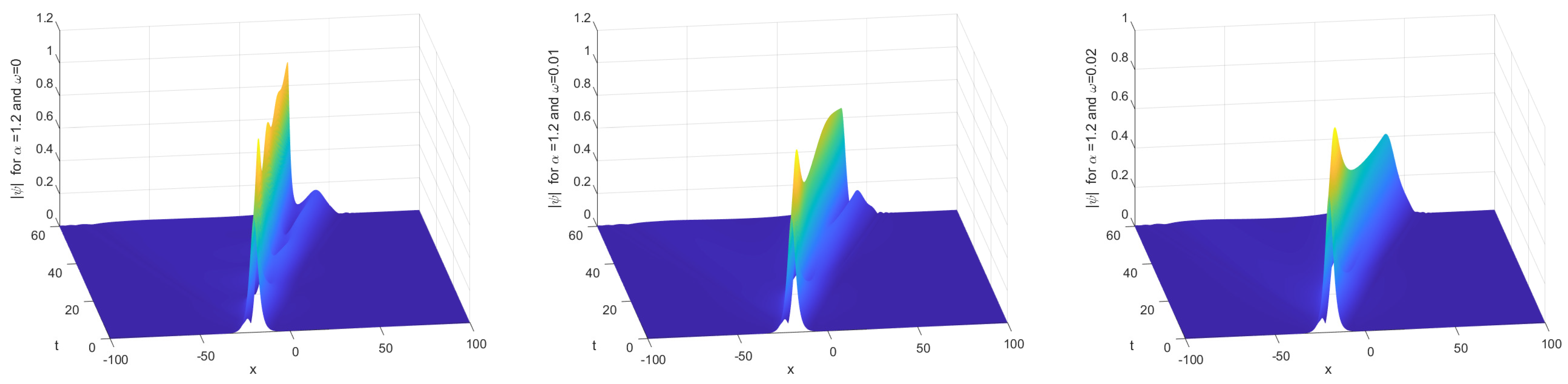
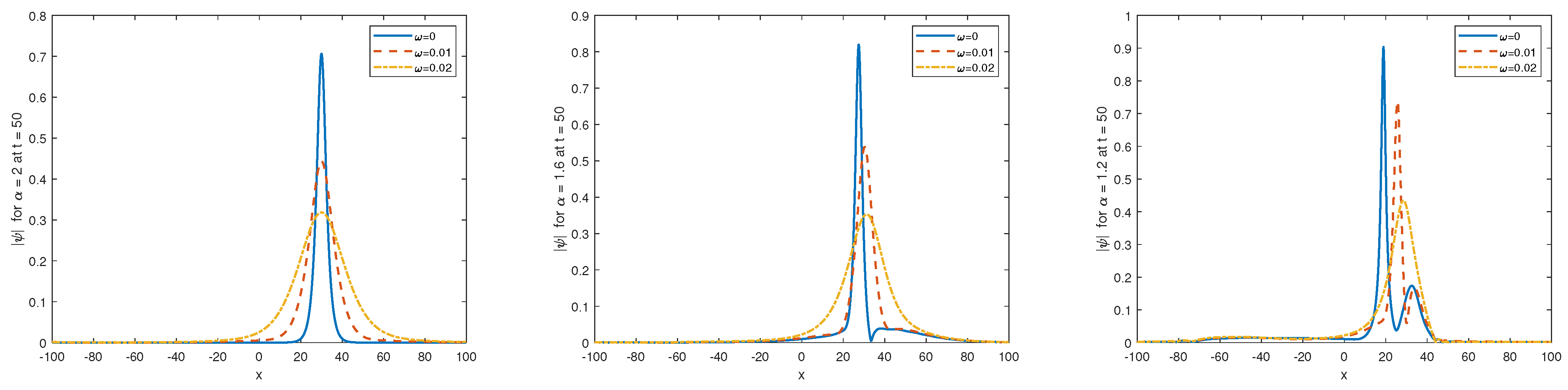
5. Numerical Experiments

In this section, we will conduct numerical experiments to validate our theoretical analysis.

Example 1.

We begin by considering the DFNLS equation:

$$\mathrm{i}{\psi }_t-{\left(-\Delta \right)}^{{\displaystyle \frac{\alpha }{2}}}\psi +2{\left|\psi \right|}^2\psi +\mathrm{i}\omega \psi =0,x\in \left(-L,L\right),0<t\le T.$$

The initial condition is given by

$$\psi \left(x,0\right)=\mathrm{sech}\left(x\right)exp\left(2\mathrm{i}x\right),x\in \left(-L,L\right).$$

In this case, we set the nonlinear oscillation parameter to $\beta =2$.

It is straightforward to verify that the initial value function $\psi (x,0)$ decays exponentially to zero as x approaches infinity. As a result, the wave function’s influence outside a sufficiently large bounded interval $[-L,L]$ is negligible. In this example, we impose the periodic boundary condition

$$\psi (-L,t)=\psi (L,t)=0,0\le t\le T,$$

with $L=20$.

First, to test the numerical accuracy of the Fourier spectral scheme (19) and (20), let ${\psi }_{ref}^n$ be the exact solution and ${\psi }_J^n$ be the numerical solution, use the error function defined as follows:

$$\mathrm{Er}\left(J,\tau \right)=\parallel {\psi }_{ref}^n-{\psi }_J^n\parallel$$

The convergence order of time can be calculated by

$${\mathrm{Rate}}_{\tau }={\displaystyle \frac{log\left(\mathrm{Er}\left(J,{\tau }_1\right)/\mathrm{Er}\left(J,{\tau }_2\right)\right)}{log\left({\tau }_1/{\tau }_2\right)}}.$$

When $\alpha =2$ and $\omega =0$, the exact solution for Example 1 can be computed explicitly as

$$\psi (x,t)=\mathrm{sech}\left(x-4t\right)exp\left(-\mathrm{i}(2x-3t)\right).$$

When $0<\alpha <2$ or $\omega >0$, the exact solution for Example 1 is not available. Therefore, we compute a reference solution $\psi$ using the Fourier spectral scheme (19) and (20), with a very small time step $\tau ={10}^{-6}$ and a sufficiently fine spatial grid $J=4800$.

Table 1. The errors and temporal convergence rates for Example 1 with $\omega =0.0$ and $J=4800$.

	$\mathit{\alpha }=1.2$		$\mathit{\alpha }=1.6$		$\mathit{\alpha }=2.0$
$\tau$	$\mathrm{Er}\left(\mathit{J},\tau \right)$	${\mathrm{Rate}}_{\tau }$	$\mathrm{Er}\left(\mathit{J},\tau \right)$	${\mathrm{Rate}}_{\tau }$	$\mathrm{Er}\left(\mathit{J},\tau \right)$	${\mathrm{Rate}}_{\tau }$
${\displaystyle \frac{1}{40}}$	4.3356 $\times {10}^{-3}$	–	9.5038 $\times {10}^{-3}$	–	8.4776 $\times {10}^{-3}$	–
${\displaystyle \frac{1}{80}}$	1.0957 $\times {10}^{-3}$	1.9843	2.3742 $\times {10}^{-3}$	2.0011	2.1081 $\times {10}^{-3}$	2.0077
${\displaystyle \frac{1}{160}}$	2.7467 $\times {10}^{-4}$	1.9962	5.9340 $\times {10}^{-4}$	2.0003	5.2631 $\times {10}^{-4}$	2.0019
${\displaystyle \frac{1}{320}}$	6.8712 $\times {10}^{-5}$	1.9990	1.4834 $\times {10}^{-4}$	2.0001	1.3153 $\times {10}^{-4}$	2.0005

and

Table 2. The errors and temporal convergence rates for Example 1 with $\omega =0.1$ and $J=4800$.

	$\mathit{\alpha }=1.2$		$\mathit{\alpha }=1.6$		$\mathit{\alpha }=2.0$
$\tau$	$\mathrm{Er}\left(\mathit{J},\tau \right)$	${\mathrm{Rate}}_{\tau }$	$\mathrm{Er}\left(\mathit{J},\tau \right)$	${\mathrm{Rate}}_{\tau }$	$\mathrm{Er}\left(\mathit{J},\tau \right)$	${\mathrm{Rate}}_{\tau }$
${\displaystyle \frac{1}{40}}$	3.1939 $\times {10}^{-3}$	–	7.7686 $\times {10}^{-3}$	–	8.4607 $\times {10}^{-3}$	–
${\displaystyle \frac{1}{80}}$	8.0681 $\times {10}^{-4}$	1.9850	1.9399 $\times {10}^{-3}$	2.0017	2.1034 $\times {10}^{-3}$	2.0080
${\displaystyle \frac{1}{160}}$	2.0222 $\times {10}^{-4}$	1.9963	4.8479 $\times {10}^{-4}$	2.0005	5.2514 $\times {10}^{-4}$	2.0020
${\displaystyle \frac{1}{320}}$	5.0587 $\times {10}^{-5}$	1.9991	1.2119 $\times {10}^{-4}$	2.0001	1.3124 $\times {10}^{-4}$	2.0005

present the temporal convergence rates at $J=2^{13}$ for various values of fractional order $\alpha$ and damping coefficient $\omega$. Both tables confirm that the proposed Fourier spectral scheme (19) and (20) achieves second-order accuracy in time, aligning with the theoretical analysis in Theorem 5. Figure 1 and Figure 2 display the errors plotted against J on a semi-logarithmic scale, with different values of $\alpha$ and $\omega$ when $\tau ={10}^{-4}$. These plots clearly demonstrate the exponential spatial convergence of the Fourier spectral scheme (19) and (20). From the figures, it is evident that for smaller $\alpha$, when $J\le 480$, the error decreases almost linearly with increasing J, and higher J values lead to smaller errors. For larger $\alpha$, the turning point in the error curve appears at smaller J values, reflecting the influence of $\alpha$ on the problem’s regularity. The figures also show that when J becomes sufficiently large, the error no longer decreases with increasing J and is instead dominated by the time discretization error. This demonstrates that the Fourier spectral scheme (19) and (20) achieves arbitrarily high accuracy for problems with sufficient smoothness.

Second, we verify the conservation properties of the Fourier spectral scheme (19) and (20). The relative errors of discrete mass and energy are defined as

$$R{M}^n=\left|{\displaystyle \frac{M^n-M^0}{M^0}}\right|,R{E}^n=\left|{\displaystyle \frac{E^n-E^0}{E^0}}\right|,$$

where $M^n$ and $E^n$ represent the mass and energy at $t=n\tau$, respectively.

We set $\tau ={10}^{-2}$ and $J=2^{10}$. Figure 3, Figure 4 and Figure 5 illustrate the relative errors of discrete mass and energy at various time points for different values of the fractional order $\alpha$ and the damping coefficient $\omega$. These results clearly demonstrate that the proposed Fourier spectral scheme (19) and (20) effectively conserves the discrete conservation laws and exhibits significant advantages.

Finally, we present a numerical comparison between our scheme (19) and (20) and Scheme I proposed in [14]. The comparison is performed for various values of the fractional order $\alpha$ and the damping coefficient $\omega$, with the spatial and temporal step sizes fixed at $J=400$ and $\tau =0.01$, respectively. The corresponding results are summarized in

Table 3. Comparison of numerical errors at $T=1$ for different values of $\alpha$ and $\omega$ with $J=400$ and $\tau =0.01$.

$\mathit{\alpha }$	$\mathit{\omega }$	Scheme	$\mathbf{Er}\left(\mathit{J},\mathit{\tau }\right)$
2.0	0.00	Scheme I [14]	3.4719 $\times {10}^{-2}$
		Scheme (19) and (20)	1.3467 $\times {10}^{-3}$
1.8	0.02	Scheme I [14]	3.1679 $\times {10}^{-3}$
		Scheme (19) and (20)	5.2487 $\times {10}^{-3}$
1.6	0.01	Scheme I [14]	3.9849 $\times {10}^{-2}$
		Scheme (19) and (20)	6.8607 $\times {10}^{-3}$

. It is evident that the proposed scheme consistently produces smaller numerical errors than Scheme I, indicating improved accuracy.

Example 2.

Next, we consider the problem described by the equation

$$\mathrm{i}{\psi }_t-{\left(-\Delta \right)}^{{\displaystyle \frac{\alpha }{2}}}\psi +\beta {\left|\psi \right|}^2\psi +\mathrm{i}\omega \psi =0,x\in \left(-L,L\right),0<t\le T.$$

The initial condition is given by

$$\psi \left(x,0\right)={\displaystyle \frac{\sqrt{2}}{2}}\mathrm{sech}\left({\displaystyle \frac{x-p}{2}}\right)exp\left(\mathrm{i}{\displaystyle \frac{x-p}{2}}\right),x\in \left(-L,L\right).$$

We apply periodic boundary conditions:

$$\psi \left(-L,t\right)=\psi \left(L,t\right)=0.$$

For this example, we set $\beta =1$ and $p=-20$.

We simulate the evolution of solitary waves in the domain $x\in [-100,100]$ and $t\in [0,60]$, with time step $\tau ={10}^{-2}$ and spatial grid number $J=2^{10}$. The results for varying fractional order $\alpha$ and damping coefficient $\omega$ are depicted in Figure 6, Figure 7 and Figure 8. A comparison of these figures reveals that as the fractional order $\alpha$ decreases, the solitary wave undergoes more rapid changes and develops additional ripples. Furthermore, a larger damping coefficient $\omega$ accelerates the dissipation of the wave. Figure 9 illustrates the soliton profiles at $t=50$ for different values of $\alpha$ and $\omega$. By comparing the solitons for $\alpha =2$ and $1<\alpha <2$, we observe the following: (1) For $\alpha =2$, the solitary wave preserves the phase space structure across the time interval $[0,60]$, regardless of the damping coefficient. In this case, $\omega$ only influences the soliton amplitude, while the waveform and wave velocity remain unaffected; (2) When $1<\alpha <2$, the soliton gradually spreads over the domain $[-100,100]$ as time progresses. As $\alpha$ decreases, the soliton’s waveform becomes more distorted. The damping coefficient $\omega$ affects not only the amplitude but also the overall shape, particularly near the soliton’s corners. Additionally, the wave velocity increases with a higher damping coefficient. These observed differences in soliton dynamics between the integer-order and fractional-order equations can be attributed to the nonlocal nature of the fractional Laplace operator.

Example 3.

Finally, we present a two-dimensional example to demonstrate the effectiveness of the proposed Fourier spectral scheme for the DFNLS equation:

$$\begin{array}{cc}\hfill & \mathrm{i}{\psi }_t(x,y,t)-{\left(-\Delta \right)}^{{\displaystyle \frac{\alpha }{2}}}\psi (x,y,t)+2{\left|\psi (x,y,t)\right|}^2\psi (x,y,t)+\mathrm{i}\omega \psi (x,y,t)=0\hfill \\ \hfill & (x,y)\in (-20,20)\times (-20,20),0<t\le T\hfill \\ \hfill & \psi \left(x,y,0\right)=\mathrm{sech}\left(x\right)\mathrm{sech}\left(y\right)exp\left(2\mathrm{i}\left(x+y\right)\right),(x,y)\in (-20,20)\times (-20,20)\hfill \\ \hfill & \psi \left(-20,y,0\right)=\psi \left(20,y,0\right),y\in (-20,20),t\in (0,T]\hfill \\ \hfill & \psi \left(x,-20,0\right)=\psi \left(x,20,0\right),x\in (-20,20),t\in (0,T]\hfill \end{array}$$

First, we evaluate the accuracy of the Fourier spectral scheme for solving two-dimensional problems. The reference “exact” solution $\psi (x,y,t)$ is obtained using a sufficiently small time step $\tau =1/5000$ and a large spatial grid with $J_x=J_y=600$. The errors as a function of $J_x$ (or $J_y$) are presented in semi-logarithmic scale in Figure 10 for different values of $\alpha$ and $\omega$. The results clearly indicate that our numerical experiments align with the theoretical analysis, confirming the spectral accuracy in space. Subsequently, Figure 11 illustrates the errors as a function of $\tau$ for varying $\alpha$ and $\omega$. It is evident that the scheme achieves second-order accuracy in time.

Next, we examine the conservation properties of the Fourier spectral scheme (19) and (20) in solving two-dimensional problems. We set $\tau =1/100$ and $J=128$. Figure 12 and Figure 13 illustrate the long-term evolution of the relative errors in mass and energy for varying fractional orders $\alpha$ and damping coefficients $\omega$. The results indicate that the Fourier spectral scheme (19) and (20) effectively preserves mass and energy conservation across different values of $\alpha$ and $\omega$ in two-dimensional scenarios.

6. Conclusions

In this paper, we derive the mass and energy conservation laws for the M-DFNLS equation and first utilize the Fourier spectral method to discretize the equation in the spatial direction. It is demonstrated that the semi-discrete system of ordinary differential equations preserves the conservation laws, and we provide a convergence analysis for this semi-discrete scheme. We then apply the Crank–Nicolson method in the time direction to develop a full-discrete scheme. This scheme is shown to be linearized and to preserve discrete mass and energy conservation laws. Furthermore, we analyze the convergence of the full-discrete scheme and investigate how the fractional order $\alpha$ and the damping coefficient $\omega$ influence the behavior of solitary solutions.

Future extensions of this work may consider numerical experiments involving rougher initial data or initial profiles with reduced regularity. Such cases are closer to real-world physical conditions and may challenge the stability and accuracy of the proposed method. Another promising direction is the application of the method to more physically meaningful scenarios, such as those arising in nonlinear optics or plasma physics, where external potentials, boundary effects, or multi-scale interactions are present. These extensions would allow for a better assessment of the method’s practical relevance and robustness. Furthermore, radial basis function (RBF) methods have recently gained attention as flexible and accurate meshless techniques for Schrödinger-type problems [26,27]. Investigating RBF-based formulations and comparing their performance with the current approach would be an interesting subject for future research.

References

1. Laskin, N. Fractional Schrödinger equation. Phys. Rev. E 2002, 66, 056108. [Google Scholar] [CrossRef] [PubMed]
2. Guo, X.; Xu, M. Some physical applications of fractional Schrödinger equation. J. Math. Phys. 2006, 47, 082104. [Google Scholar] [CrossRef]
3. Longhi, S. Fractional Schrödinger equation in optics. Opt. Lett. 2015, 40, 1117–1120. [Google Scholar] [CrossRef]
4. Zhang, L.; Li, C.; Zhong, H.; Xu, C.; Lei, D.; Li, Y.; Fan, D. Propagation dynamics of super-Gaussian beams in fractional Schrödinger equation: From linear to nonlinear regimes. Opt. Express. 2016, 24, 14406–14418. [Google Scholar] [CrossRef]
5. Ionescu, A.D.; Pusateri, F. Nonlinear fractional Schrödinger equations in one dimension. J. Funct. Anal. 2014, 266, 139–176. [Google Scholar] [CrossRef]
6. Pozrikidis, C. The Fractional Laplacian; Chapman and Hall/CRC: New York, NY, USA, 2016. [Google Scholar]
7. Tsutsumi, M. Nonexistence of global solutions to the Cauchy problem for the damped nonlinear Schrödinger equations. SIAM J. Math. Anal. 1984, 15, 357–366. [Google Scholar] [CrossRef]
8. Fu, H.; Zhou, W.; Qian, X.; Song, S.H.; Zhang, L.Y. Conformal structure-preserving method for damped nonlinear Schrödinger equation. Chin. Phys. B 2016, 25, 110201. [Google Scholar] [CrossRef]
9. Fu, H.; Zhou, W.; Qian, X.; Song, S. Novel conformal structure-preserving algorithms for coupled damped nonlinear Schrödinger system. Adv. Appl. Math. Mech. 2017, 9, 1383–1403. [Google Scholar] [CrossRef]
10. Jiang, C.; Cai, W.; Wang, Y. Optimal error estimate of a conformal Fourier pseduo-spectral method for the damped nonlinear Schrödinger equation. Numer. Methods Partial. Differ. Equ. 2018, 34, 1422–1454. [Google Scholar] [CrossRef]
11. Wang, T.; Wang, J.; Guo, B. Two completely explicit and unconditionally convergent Fourier pseudo-spectral methods for solving the nonlinear Schrödinger equation. J. Comput. Phys. 2020, 404, 109116. [Google Scholar] [CrossRef]
12. Tarek, S. Remarks on damped fractional Schrödinger equation with pure power nonlinearitys. J. Math. Phys. 2015, 56, 061502. [Google Scholar]
13. Liang, J.; Song, S.; Zhou, W.; Fu, H. Analysis of the damped nonlinear space-fractional schrödinger equation. Appl. Math. Comput. 2018, 320, 495–511. [Google Scholar] [CrossRef]
14. Fu, Y.; Song, Y.; Wang, Y. Maximum-norm error analysis of a conservative scheme for the damped nonlinear fractional Schrödinger equation. Math. Comput. Simul. 2019, 166, 206–223. [Google Scholar] [CrossRef]
15. Wu, L.; Ma, Q.; Ding, X. Conformal structure-preserving method for two-dimensional damped nonlinear fractional Schrödinger equation. Numer. Methods Partial Differ. Equ. 2023, 39, 3195–3221. [Google Scholar] [CrossRef]
16. Ding, H.; Qu, H.; Yi, Q. Construction and analysis of structure-preserving numerical algorithm for two-dimensional damped nonlinear space fractional Schrödinger equation. J. Sci. Comput. 2024, 99, 60. [Google Scholar] [CrossRef]
17. Fei, M.; Huang, C.; Wang, P. Error estimates of structure-preserving Fourier pseudospectral methods for the fractional Schrödinger equation. Numer. Methods Partial Differ. Equ. 2019, 36, 369–393. [Google Scholar] [CrossRef]
18. Wang, Y.; Mei, L.; Bu, L. Split-step spectral Galerkin method for the two-dimensional nonlinear space-fractional Schrödinger equation. Appl. Numer. Math. 2019, 136, 257–278. [Google Scholar] [CrossRef]
19. Zou, G.; Wang, B.; Sheu, T. On a conservative Fourier spectral Galerkin method for cubic nonlinear Schrödinger equation with fractional Laplacian. Math. Comput. Simul. 2020, 168, 122–134. [Google Scholar] [CrossRef]
20. Abdolabadi, F.; Zakeri, A.; Amiraslani, A. A split-step Fourier pseudo-spectral method for solving the space fractional coupled nonlinear Schrödinger equations. Commun. Nonlinear Sci. Numer. Simul. 2023, 120, 107150. [Google Scholar] [CrossRef]
21. Lawson, J. Generalized Runge-Kutta processes for stable systems with large Lipschitz constants. SIAM J. Numer. Anal. 2006, 4, 372–380. [Google Scholar] [CrossRef]
22. Wang, P.; Huang, C. Structure-preserving numerical methods for the fractional Schrödinger equation. Appl. Numer. Math. 2018, 129, 137–158. [Google Scholar] [CrossRef]
23. Li, C. Numerical Analysis for Some Fractional Anomalous Diffusion Equations. Ph.D. Thesis, Lanzhou University, Lanzhou, China, 2009. [Google Scholar]
24. Wang, J.; Xiao, A. Conservative Fourier spectral method and numerical investigation of space fractional Klein-Gordon-Schrödinger equations. Appl. Math. Comput. 2019, 350, 348–365. [Google Scholar] [CrossRef]
25. Shen, J.; Tang, T.; Wang, L. Spectral Methods: Algorithms, Analysis and Applications; Springer: Berlin/Heidelberg, Germany, 2010. [Google Scholar]
26. Noorizadegan, A.; Chen, C.; Young, D.; Chen, C. Effective condition number for the selection of the RBF shape parameter with the fictitious point method. Appl. Numer. Math. 2022, 178, 280–295. [Google Scholar] [CrossRef]
27. Tian, J.; Ding, H. Improved high-order difference scheme for the conservation of mass and energy in the two-dimensional spatial fractional Schrödinger equation. Fractal Fract. 2025, 9, 280. [Google Scholar] [CrossRef]
Figure 1. The errors and spatial accuracy for Example 1 with ω = 0.0 and time step τ = 10 4 .
Fractalfract 09 00328 g001
Figure 2. The errors and spatial accuracy for Example 1 with ω = 0.1 and time step τ = 10 4 .
Fractalfract 09 00328 g002
Figure 3. The relative mass and energy errors for Example 1 with ω = 0 and different α .
Fractalfract 09 00328 g003
Figure 4. The relative mass and energy errors for Example 1 with ω = 0.01 and different α .
Fractalfract 09 00328 g004
Figure 5. The relative mass and energy errors for Example 1 with ω = 0.02 and different α .
Fractalfract 09 00328 g005
Figure 6. Evolution of the solitons for Example 2 with α = 2.0 and different damping coefficients ω .
Fractalfract 09 00328 g006
Figure 7. Evolution of the solitons for Example 2 with α = 1.6 and different damping coefficients ω .
Fractalfract 09 00328 g007
Figure 8. Evolution of the solitons for Example 2 with α = 1.2 and different damping coefficients ω .
Fractalfract 09 00328 g008
Figure 9. Solitons for Example 2 at t = 50 with different fractional order α and damping coefficients ω .
Fractalfract 09 00328 g009
Figure 10. The errors for Example 3 with ω = 0 (left), ω = 0.5 (right) and τ = 1 / 5000 .
Fractalfract 09 00328 g010
Figure 11. The errors for Example 3 with ω = 0 (left), ω = 0.5 (right) and J x = J y = 600 .
Fractalfract 09 00328 g011
Figure 12. The relative mass and energy errors with ω = 0 for different α .
Fractalfract 09 00328 g012
Figure 13. The relative mass and energy errors with ω = 0.02 for different α .
Fractalfract 09 00328 g013