Skewed Multifractal Cross-Correlations Between Green Bond Index and Energy Futures Markets: A New Perspective Based on Change Point

Abstract

This study is the first to use the Bayesian Estimator of Abrupt Change, Seasonality, and Trend (BEAST) algorithm to detect trend change points in the nexuses between the green bond index (Green Bond) and WTI of crude oil, gasoline, as well as natural gas futures. The COVID-19 pandemic and the Russia–Ukraine war are identified as common significant trend change points, and the total sample is subsequently divided into three stages based on these points. Utilizing a skewed MF-DCCA method, this study analyzed the skewed multifractal characteristics between the Green Bond and the energy futures across these stages. The results revealed that both the multifractal characteristics and risk levels experienced significant changes across different periods, exhibiting skewed multifractality. Specifically, from the pre-pandemic period to the post-Russia–Ukraine conflict period, the multifractal features and risk of the Green Bond and WTI and Green Bond and Gasoline groups first declined and then increased, while the Green Bond and Natural Gas group displayed an opposite trend, showing an initial increase followed by a decline. A portfolio analysis further indicated that Green Bond provided effective hedging against all three types of energy futures, particularly during crisis periods. Notably, the portfolios constructed using the Mean-MF-DCCA model, which incorporated multifractal features, outperformed those constructed by traditional portfolio models. These findings offered new insights into the dynamic characteristics of the Green Bond and energy futures markets and provided important policy implications for portfolio optimization and risk management strategies.

1. Introduction

In recent years, the global issue of environmental degradation has become increasingly severe [1], which fosters a broad consensus on the imperative of pursuing sustainable, green, and low-carbon development [2]. As an important financial instrument for advancing a low-carbon economy and promoting environmental protection, Green Bond has increasingly attracted widespread attention from international investors and issuers. Although Green Bond shares the same credit risk characteristics as conventional bonds, they have a more substantial capacity to withstand market stress. This resilience is largely attributed to the composition of their investor base, which primarily consists of long-term institutional investors such as pension funds, mutual funds, insurance companies, and multilateral development institutions like the World Bank. In addition, Green Bond issuers are typically large, highly rated, and financially stable organizations, which tend to possess greater crisis management capabilities and demonstrate stronger resilience during periods of market turbulence [3].

Many studies have examined the relationship between Green Bond and energy commodities with the sharp volatility in global energy prices, particularly in crude oil. For instance, Naeem et al. [4] employed the Cross-Quantilogram approach to investigate the nonlinear and asymmetric dependencies between Green Bond and various energy commodities, emphasizing their behavior under extreme market conditions. Huang et al. [5] applied the DCC-GARCH model and reported a negative correlation between Green Bond and crude oil during the COVID-19 pandemic and the Russia–Ukraine conflict. Furthermore, Naeem et al. [3] demonstrated the existence of asymmetric upper- and lower-tail dependencies between Green Bond and multiple energy commodities using a time-varying optimal Copula model. In addition, studies based on TVP-VAR models [6,7,8] have shown that the spillover effects between Green Bond and crude oil are time-varying and primarily influenced by major international or domestic events. Overall, empirical evidence confirms a complex relationship between energy commodities and Green Bond, which evolves in response to various influencing factors.

However, the global COVID-19 pandemic and the outbreak of the Russia–Ukraine war have reshaped global supply chains and the energy trade landscape. Additionally, through the complex interactions of policy transmission, market sentiment, and risk pricing, these events have given rise to nonlinear characteristics in financial markets that traditional theories struggle to explain. According to the 2023 report by the Bank for International Settlements (BIS), the global Green Bond market expanded to $1.7 trillion over the three years following the pandemic, while the annualized volatility of energy futures prices during the same period increased by 62% compared to the pre-pandemic average. This seemingly paradoxical coexistence of a “green premium” and “fossil energy volatility” exposes the fundamental limitations of traditional linear analytical frameworks in explaining market heterogeneity. Against this backdrop, analyzing the multifractal cross-correlations between Green Bond and energy futures markets, along with their dynamic patterns before and after change points such as the COVID-19 pandemic and the Russia–Ukraine war, will not only promote interdisciplinary innovation between financial economics and complexity science but also provide a scientific basis for building resilient low-carbon financial infrastructure and preventing systemic risk contagion across markets.

This study presents several innovations: First, this study is the first to apply the BEAST algorithm to examine trend change points in the nexuses between the Green Bond and energy futures, which offers high accuracy. Second, this study applied the newly proposed skewed MF-DCCA method [9] to examine the skewed multifractal cross-correlations between Green Bond and major energy futures for the first time. It compared the multifractal characteristics and risk levels of the two markets before and after the COVID-19 pandemic and the Russia–Ukraine war, explored the underlying drivers of these dynamics, and provided new evidence on their evolving interactions under different market conditions. Finally, in contrast to existing research [9], this study further incorporated the results of the skewed MF-DCCA into portfolio construction by applying the Mean-MF-DCCA portfolio model, which enabled a systematic assessment of the hedging effectiveness of Green Bond and demonstrated superior risk-adjusted performance compared to the conventional Markowitz model. These findings have significant implications for optimizing portfolio allocation and formulating effective risk management strategies.

2. Literature Review

Early financial market analyses were primarily based on Fama’s Efficient Market Hypothesis (EMH) [10]. However, an increasing body of empirical research suggests that financial markets are not fully efficient and exhibit significant nonlinear characteristics [11]. Then, Benoit B. Mandelbrot proposed the Fractal Market Hypothesis in 1997 to explain the complexity and volatility of financial markets. This hypothesis revitalized research in financial markets and established a robust groundwork for the subsequent application of fractal geometry in the financial domain. Fractal theory and multifractal analysis have been widely introduced in financial market research to identify complex behaviors and localized fluctuations across different time scales [12]. In 1994, Peng et al. [13] developed Detrended Fluctuation Analysis (DFA), which effectively detects long-range correlations in financial time series. Later, to analyze the cross-correlations between two different time series, Podobnik and Stanley [14] introduced Detrended Cross-Correlation Analysis (DCCA) in 2008. Compared with conventional non-fractal approaches, these methods not only allow for detecting long-memory effects but also exhibit strong adaptability to non-stationary time series. However, both DFA and DCCA were limited to study monofractal structures. To address this limitation, Kantelhardt et al. [15] extended DFA to Multifractal Detrended Fluctuation Analysis (MF-DFA), enabling it to characterize time series with multifractal properties. This method quickly gained widespread applications in financial research. For example, Leandro dos Santos Maciel [16], Telli [17], and Gu et al. [18] applied the MF-DFA method to analyze the multifractal characteristics of stock markets, cryptocurrency markets, and economic policy uncertainty, respectively. Meanwhile, Zhou [19] extended DCCA to Multifractal Detrended Cross-Correlation Analysis (MF-DCCA), facilitating the detection of multifractal cross-correlations between two time series. Subsequent studies applied MF-DCCA to the agricultural futures markets of China and the United States [20], major Brazilian inflation indices [21], and the corn futures markets of China and the United States [22]. Their analysis consistently confirmed the presence of multifractal cross-correlations.

A growing number of studies have begun to examine the multifractal characteristics of Green Bond and energy futures. However, several limitations remain in the existing literature. First, most studies focus on examining the multifractal cross-correlations between Green Bond and traditional U.S. bonds or stock indices [23] or exploring the multifractal cross-correlations between different energy futures [24]. However, limited research has examined the multifractal cross-correlations between Green Bond and specific energy futures. Second, although Gokten et al. [25] applied the MF-DCCA method to investigate the multifractal cross-correlations between Green Bond and several major commodity indices, including an energy commodity index, their analysis was primarily conducted at the macro level. Their analysis has not yet been extended to specific major energy commodities, nor has it fully considered the impact of significant external shocks such as the COVID-19 pandemic and the Russia–Ukraine war. Emerging evidence [26,27] suggests that the COVID-19 pandemic and geopolitical conflicts have significantly influenced the multifractal cross-correlations between markets. These findings imply that the pandemic and the Russia–Ukraine war will likely affect the multifractal cross-correlations between Green Bond and energy futures, potentially resulting in skewed multifractality. Therefore, this study employed the skewed MF-DCCA method to identify structural change points in the cross-correlations between Green Bond and energy futures and examined their impact on multifractal characteristics. In addition, the multifractal characteristics were incorporated into the portfolio model, and the Mean-MF-DCCA method was applied to analyze the portfolios between Green Bond and energy futures.

3. Skewed Multifractal Analysis Methodology

The skewed analysis approach is a new multifractal analysis approach that extends the standard MF-DCCA by incorporating change point detection. This methodological innovation is inspired by the core idea of the skewed MF-DFA method introduced by Oświęcimka [28]. He noted that traditional multifractal methods typically assume a uniform multifractal structure throughout the entire time series, neglecting potential structural shifts. However, in real-world financial markets, abrupt external shocks such as global crises often induce significant changes in market behavior, affecting the multifractal properties of financial time series [24]. By introducing change point detection into multifractal analysis, the skewed method allows for a more accurate assessment of how major events, such as the COVID-19 pandemic, influence the multifractal structure. For instance, using this skewed approach, Oświȩcimka [28] detected and confirmed significant changes in the multifractality of stock markets in the G3 + 1 countries during the COVID-19 period. Moreover, he demonstrated pronounced skewed multifractal features in three major North African stock indices (EGX30, MASI, and Tunindex) over the 2010–2023 period, attributable to major regional and global events [29]. These empirical findings highlight the effectiveness of the skewed method and emphasize its value as a necessary improvement over the traditional multifractal approach.

Therefore, to further improve the traditional MF-DCCA method, this study proposes the skewed multifractal cross-correlation approach. This advancement extends the skewed MF-DFA method to the analysis of cross-correlations and enhances the detection of structural changes in financial time series by employing the BEAST method.

The skewed multifractal analysis in this study follows four main steps. First, the BEAST method is applied to detect change points accurately. Second, the original time series is segmented according to the identified change points. Third, the MF-DCCA method is applied to each segment. Finally, the multifractal characteristics of each segment are compared to assess whether the cross-correlations display skewed behavior before and after the structural changes. If the multifractal properties between two adjacent subsequences differ, it indicates the presence of skewed multifractal cross-correlations.

3.1. Change Point Test

The change points refer to points where the structure of the series changes, typically indicating significant shifts in market behavior or characteristics before and after these points. Identifying and analyzing these change points is crucial in financial research, as it aids in investment decision-making, risk management, asset allocation, and understanding financial markets. This study applies the BEAST algorithm [30] to identify abrupt changes in financial markets, which may include major international events, policy adjustments, market structure shifts, or changes in economic conditions. Existing literature has demonstrated that the BEAST algorithm can effectively detect structural changes in various types of time series, such as those in environmental and medical fields [31,32]. Given the comparable complexity and structural dynamics of financial time series, the BEAST method is also well-suited for applications in financial research [30]. Moreover, compared with conventional change point detection methods, BEAST has shown superior performance in both detection accuracy and the characterization of structural shifts [33,34]. Therefore, the use of BEAST in this study is justified by its methodological advantages and suitability for the data. It enables more accurate identification of structural changes, critical for analyzing the evolving relationship between Green Bond and energy futures.

The following section briefly presents the formulas used in the BEAST algorithm.

Given a time series $D={\left\{t_i,y_i\right\}}_{i=1,\dots ,n}$ consisting of seasonality, trend, and abrupt changes, the calculation formula is as follows:

$$y_i=S\left(t_i;{⊝}_s\right)+T\left(t_i;{⊝}_T\right)+{\epsilon }_i$$

(1)

Assume that the noise ε_i follows a Gaussian distribution and represents the portion of ${\mathit{y}}_{\mathit{i}}$ that cannot be explained by the seasonal component $S\left(t_i;{⊝}_s\right)$ and the trend component $T\left(t_i;{⊝}_T\right)$.

Specifically, the $S\left(t\right)$ component is approximated by a piecewise harmonic model featuring q points located at times ${\epsilon }_k(\mathrm{w}\mathrm{h}\mathrm{e}\mathrm{r}\mathrm{e}k=1,\dots ,q)$. Then, those points segment the series into (q + 1) sub-series $\left[{\epsilon }_k,{\epsilon }_{k+1}\right](k=0,\dots ,q)$. When k = 0, ${\mathit{\epsilon }}_0$ is the beginning of the series, and when k = q, ${\epsilon }_{q+1}$ is the end time of the series. For each interval, the $S\left(t\right)$ component can be computed as follows:

$$S\left(t\right)=\sum _{i=1}^{H_k}\left[a_{k,h}·sin\left({\displaystyle \frac{2\pi ht}{P}}\right)+b_{k,h}·cos\left({\displaystyle \frac{2\pi ht}{P}}\right)\right]$$

(2)

where ${\epsilon }_k\le t<{\epsilon }_{k+1},k=0,\dots ,q$.

The period P refers to the duration of the seasonal component (typically set to 1 year). The symbol $H_k$ signifies the harmonic index for the k-th sub-series. These parameters $\left\{a_{k,h},b_{k,h}\right\}$ represent the coefficients corresponding to the sine and cosine components. Overall, the model is discontinuous, with points ${\epsilon }_k$ presenting potential change points where seasonal shifts may occur. The q represents the amount of change points, and $\left\{{\epsilon }_k\right\}$ are the time points, all of which are unknown parameters. To define the seasonal harmonic curve, the following parameters need to be estimated:

$${⊝}_s=\left\{q\right\}\cup {\left\{{\epsilon }_k\right\}}_{k=1,\dots ,q}\cup {\left\{H_k\right\}}_{k=0,\dots ,q}\cup {\left\{a_{k,h},b_{k,h}\right\}}_{k=0,\dots ,q,h=1,\dots ,H_k}$$

(3)

The trend component is characterized as a segmented linear function. It consists of u points located at ${\theta }_j(j=1,\dots ,u)$. Then, we obtain (u + 1) sub-series $\left[{\theta }_j,{\theta }_{j+1}\right](j=0,\dots ,u)$. Similarly, ${\theta }_0$ and ${\theta }_{u+1}$ correspond to the beginning and end of the series, respectively. The trend change points ${\theta }_j$ do not have to coincide with the seasonal change points ${\epsilon }_k$. For each interval, the trend is given by

$$\mathit{T}\left(\mathit{t}\right)\mathit{=}{\mathit{a}}_{\mathit{j}}\mathit{+}{\mathit{b}}_{\mathit{j}}\mathit{t}$$

(4)

where ${\theta }_j\le t<{\theta }_{j+1},j=0,\dots ,u$.

Similarly, the harmonic curve of the T component is given by

$${⊝}_T=\left\{u\right\}\cup {\left\{{\theta }_j\right\}}_{j=1,\dots ,u}\cup {\left\{a,b_j\right\}}_{j=0,\dots ,u}$$

(5)

The parameters ${⊝}_s$ and ${⊝}_T$ must be derived from the data D. Here, these two sets of parameters are grouped into $\left\{{⊝}_s,{⊝}_T\right\}=\left\{M,{\beta }_M\right\}$. M denotes the structure of model and is composed of the following parameters:

$$M=\left\{u\right\}\cup {\left\{{\theta }_j\right\}}_{j=1,\dots ,u}\cup \left\{q\right\}\cup {\left\{{\epsilon }_k\right\}}_{k=1,\dots ,q}\cup {\left\{H_k\right\}}_{k=0,\dots ,q}$$

(6)

The ${\beta }_M$ determines the shape of the seasonal and trend curves. The expression for ${\beta }_M$ is as follows:

$${\beta }_M={\left\{a_{k,h},b_{k,h}\right\}}_{k=0,\dots ,q,h=1,\dots ,H_k}\cup {\left\{a,b_j\right\}}_{j=0,\dots ,u}$$

(7)

At this time, the original Equation (1) becomes

$$y\left(t_i\right)=x_M\left(t_i\right){\beta }_M+{\epsilon }_i$$

(8)

Next, it is necessary to establish the structure of model M. Once M is established, the coefficients ${\mathit{\beta }}_{\mathit{M}}$ can be estimated. Given the large number of possible model structures, Bayesian inference is used to address this extensive problem.

Bayesian models can be derived by extending Equations (1) or (8) to detect seasonality, trend, and abrupt changes. In this model, all unspecified parameters are considered random variables. For a given time series $D={\left\{t_i,y_i\right\}}_{i=1,\dots ,n}$, we need to obtain the optimal parameters values and the posterior $p\left({\beta }_M,{\sigma }^2,M|D\right)$. This distribution can be obtained as follows:

$$p\left({\beta }_M,{\sigma }^2,M|D\right)\propto p\left(D|{\beta }_M,{\sigma }^2,M\right)\pi \left({\beta }_M,{\sigma }^2,M\right)$$

(9)

where $p\left(D|{\beta }_M,{\sigma }^2,M\right)$ is the likelihood, representing the probability of observing the data D given the parameters ${\beta }_M,{\sigma }^2,$ and $M$. As ε adheres to a normal distribution, $p\left(D|{\beta }_M,{\sigma }^2,M\right)$ also adheres to a Gaussian distribution: $p\left(D|{\beta }_M,{\sigma }^2,M\right)={\prod }_{i=1}^{n}N(y_i;x_M\left(t_i\right){\beta }_M,{\sigma }^2)$. The prior distribution of these parameters is denoted as $\pi \left({\beta }_M,{\sigma }^2,M\right)$ and is expressed as follows:

$$\pi \left({\beta }_M,{\sigma }^2,M\right)=\pi \left({\beta }_M,{\sigma }^2|M\right)\pi \left(M\right)$$

(10)

The prior distribution can be obtained as long as the conditional prior $\pi \left({\beta }_M,{\sigma }^2|M\right)$ and the model prior $\pi \left(M\right)$ are derived, assuming a flat prior. Given the probability and prior model, the posterior distribution regarding the model parameters is as follows:

$$p\left({\beta }_M,{\sigma }^2,\lambda ,M|D\right)\propto \prod _{i=1}^{n}N\left(y_i;x_M\left(t_i\right){\beta }_M,{\sigma }^2\right)·{\pi }_{\beta }\left({\beta }_M,{\sigma }^2,\lambda |M\right)\pi \left(M\right)$$

(11)

The core formulation and model are outlined here, further details can be found in [30]. The source code is available at http://github.com/zhaokg/Rbeast, accessed on 16 March 2025.

3.2. Skewed Multifractal Cross-Correlation Analysis

Once change points are detected, this paper first divides the original time series into several subsequences based on these change points. Subsequently, the MF-DCCA approach is employed independently for each sub-interval. If the scaling behavior of the adjacent subsequences differs, skewed multifractality exists. The steps involved are described below:

Step 1: Consider two time series, t = 1, 2, …, N, where N represents the length of the series.

$$X\left(t\right)=\sum _{k=1}^t\left(x\left(k\right)-\overline{x}\right),Y\left(t\right)=\sum _{k=1}^t\left(y\left(k\right)-\overline{y}\right)$$

(12)

and $\overline{x}$ and $\overline{y}$ are the means of the sequences $x\left(k\right)$ and $y\left(k\right)$, respectively.

Step 2: Divide {$X\left(t\right)$} and {$Y\left(t\right)$} into $N_s=int\left({\displaystyle \frac{N}{s}}\right)$ non-overlapping segments of equal length s, where N is the total length of the series. Since N is not always an integer multiple of s, the process is repeated from the end of the series to avoid losing data. As a result, a total of 2$N_s$ subsequences are obtained.

Step 3: For each subinterval $\gamma$, apply the least squares method to fit $X_{\gamma }$ and $Y_{\gamma }$ using an m-order polynomial. In line with most of the related literature [23], a second-order polynomial is used here. For $\gamma$= 1, 2, …, N_s, the detrended covariance function is as follows:

$$F^2\left(s,\gamma \right)={\displaystyle \frac{1}{s}}\sum _{i=1}^s\left|X\left[\left(\gamma -1\right)s+i\right]-\widetilde{X_{\gamma }\left(i\right)}\right|\times \left|Y\left[\left(\gamma -1\right)s+i\right]-\widetilde{Y_{\gamma }\left(i\right)}\right|$$

(13)

and when $\gamma$= Ns + 1, …, 2Ns,

$$F^2\left(s,\gamma \right)={\displaystyle \frac{1}{s}}\sum _{i=1}^s\left|X\left[N-\left(\gamma -N_S\right)s+i\right]-\widetilde{X_{\gamma }\left(i\right)}\right|\times \left|Y\left[N-\left(\gamma -N_S\right)s+i\right]-\widetilde{Y_{\gamma }\left(i\right)}\right|$$

(14)

where $\widetilde{X_{\gamma }\left(i\right)}$ and $\widetilde{Y_{\gamma }\left(i\right)}$ represent the fitted polynomials for each segment $\mathit{\gamma }$.

Step 4: The fluctuation function can be obtained as follows:

$$F_q\left(s\right)={\left\{{\displaystyle \frac{1}{2N_s}}\sum _{\gamma =1}^{2N_s}[F^2\left(s,\gamma \right){]}^{{\displaystyle \frac{q}{2}}}\right\}}^{{\displaystyle \frac{1}{q}}}\left(q\ne 0\right)$$

(15)

And when q = 0,

$$F_0\left(s\right)=exp\left\{{\displaystyle \frac{1}{4N_s}}\sum _{\gamma =1}^{2N_s}\mathit{ln}\left[F^2\left(s,\gamma \right)\right]\right\}$$

(16)

Step 5: By plotting the fluctuation function $F_q\left(s\right)$ against s on a double logarithmic scale, we can observe the scaling behavior for various q-values. If a long-range cross-correlation exists between the series $x_t$ and $y_t$, the fluctuation function will exhibit a scaling relationship.

$$F_q\left(s\right)~s^{H_{xy}\left(q\right)}$$

(17)

By employing the OLS method to regress log$F_q\left(s\right)$ against log(s), the generalized Hurst exponent $H_{xy}\left(q\right)$ is obtained. If $H_{xy}\left(q\right)$ is different with changing values of q, it indicates the presence of multifractal cross-correlation. Specifically, the $H_{xy}\left(2\right)$ index serves as the Hurst exponent, reflecting the persistence of long-range correlations. The Hurst exponent value greater than 0.5 indicates persistent cross-correlation, whereas a value less than 0.5 suggests anti-persistence. If $H_{xy}\left(2\right)=0.5$, it implies the absence of a cross-correlation between the sequences. Additionally, the $∆H$ index derived from the generalized Hurst exponent quantifies the degree of multifractality.

$$∆H={H_{xy}\left(q\right)}_{max}-{H_{xy}\left(q\right)}_{min}$$

(18)

If the $∆H$ index is larger, it indicates stronger multifractality. The relationship between the multifractal scaling index ${\tau }_{xy}\left(q\right)$ and the generalized Hurst exponent is as follows:

$${\tau }_{xy}\left(q\right)=q·h_{xy}\left(q\right)-1$$

(19)

If ${\tau }_{xy}\left(q\right)$ shows a linear relationship with q, then the cross-correlation between the two time series is monofractal. Otherwise, it is multifractal. Through the Legendre transformation, the following can be obtained:

$${\alpha }_{xy}\left(q\right)=H_{xy}\left(q\right)+q{H}_{xy}^{\prime }\left(q\right)$$

(20)

$$f_{xy}\left(\alpha \right)=q\left[\alpha -H_{xy}\left(q\right)\right]+1$$

(21)

where $\mathit{\alpha }$ represents the singularity index, and $f_{xy}\left(\alpha \right)$ denotes the multifractal spectrum. Additionally, the range of ${\alpha }_{xy}\left(q\right)$ can be calculated to quantify the degree of multifractality.

$${∆\alpha }_{xy}\left(q\right)={{\alpha }_{xy}\left(q\right)}_{max}-{{\alpha }_{xy}\left(q\right)}_{min}$$

(22)

The larger ${∆\alpha }_{xy}\left(q\right)$, the stronger the multifractal features and fluctuations.

Additionally, this paper utilizes the MRCC method [21] to assess the multifractal risk degree $\mathit{\Gamma }$. The $\mathit{\Gamma }$ statistic is computed as follows, where ${\mathit{W}}_{\mathit{x}\mathit{y}}$ denotes the width of the multifractal spectrum (i.e., ${∆\alpha }_{xy}\left(q\right)$), and ${\mathit{\alpha }}_{\mathit{x}\mathit{y}}\left(\mathit{0}\right)$ represents the ${\mathit{\alpha }}_{\mathit{x}\mathit{y}}$ value corresponding to the maximum of the $f_{xy}\left(\alpha \right)$:

$$\mathit{\Gamma }\mathit{=}\frac{{\mathit{W}}_{\mathit{x}\mathit{y}}}{{\mathit{\alpha }}_{\mathit{x}\mathit{y}}\left(\mathit{0}\right)}$$

(23)

A larger MRCC statistic value indicates that the cross-correlation between the two time series is more complex and persistent, reflecting lower market efficiency and greater multifractal risk. This method provides a macroeconophysics perspective for managing market efficiency and risk.

3.3. Mean MF-DCCA Portfolio Construction

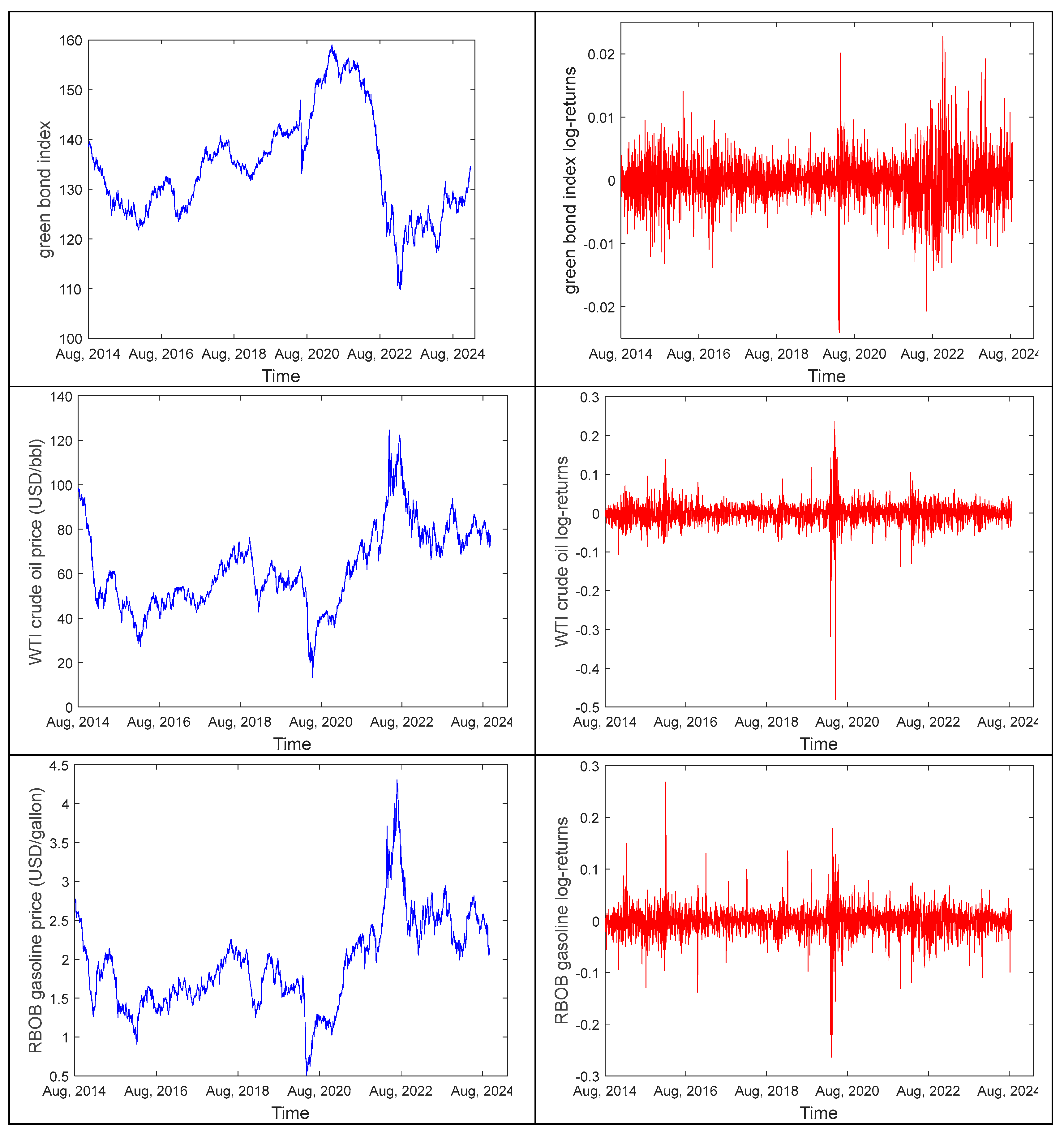
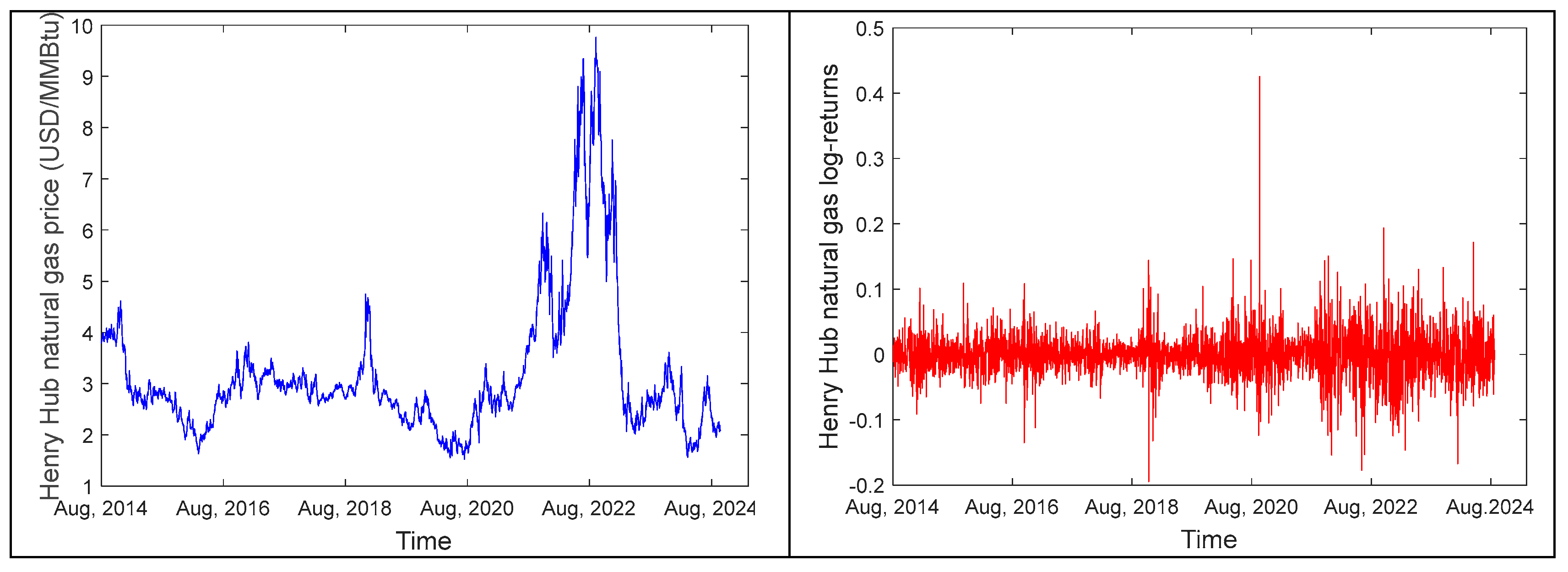
The traditional mean-variance model is primarily based on the Markowitz framework. The model is formulated as follows:

Assume that the portfolio is composed of N risky assets. The return of the portfolio $R_p$ is defined as the weighted average of the returns of the individual assets:

$$R_p=\sum _{i=1}^N{w}_i{R}_i$$

(24)

where $w_i$ denotes the weight of asset i (i = 1, …, N), and $R_i$ represents the return of asset i. The weights satisfy $\sum _{i=1}^N{w}_i=1,w_i\ge 0$. The expected return $E\left(R_p\right)$ and the variance ${\sigma }^2\left(R_p\right)$ of the portfolio are calculated as follows:

$$E\left(R_p\right)=\sum _{i=1}^N{w}_{i}E\left(R_i\right)$$

(25)

$${\sigma }^2\left(R_p\right)=\sum _{i=1}^N\sum _{j=1}^N{w}_i{w}_j{\sigma }_{ij}$$

(26)

where $E\left(R_i\right)$ denotes the expected return of asset i, and ${\sigma }_{ij}$ represents the covariance between the returns of assets i and j.

The following are the objective functions for the minimum-variance portfolio, maximum Sharpe ratio portfolio, and minimum downside risk portfolio, with the goal being to adjust the asset weights to minimize portfolio risk or maximize portfolio return. The risk-free rate $R_f$ is represented by the 10-year U.S. Treasury bond yield.

$$\begin{array}{c}\begin{array}{c}\begin{array}{c}Minimize{\displaystyle \sum _{i=1}^N}{\displaystyle \sum _{j=1}^N}{w}_i{w}_j{\sigma }_{ij}\\ orMaximizeSharperatio={\displaystyle \frac{E\left(R_p\right)-R_f}{\sigma \left(R_p\right)}}={\displaystyle \frac{{\sum }_{i=1}^N{w}_{i}E\left(R_i\right)-R_f}{\sqrt{{\sum }_{i=1}^N{\sum }_{j=1}^N{w}_i{w}_j{\sigma }_{ij}}}}\end{array}\\ orMinimize\sqrt{{\displaystyle \frac{{\sum }_{i=1}^N{\left[min\left(0,{\sum }_{i=1}^N{w}_i{R}_i\right)\right]}^2}{N}}}\end{array}\\ s.t.{\displaystyle \sum _{i=1}^N}{w}_i=1,w_i\ge 0,i=1,\dots ,N\end{array}$$

(27)

The optimal weights $w_i$ for these portfolios are obtained through quadratic programming.

To incorporate multifractal cross-correlations into portfolio construction, we employ the Mean MF-DCCA portfolio model previously proposed [35] under the Reward–Risk Criterion (RRC) framework.

Suppose portfolio A comprises m risky assets $\left\{Y_i\right\}$ (i = 1, …, m). Let $E\left(R_i\right)$ denote the expected return of asset $Y_i$, and let $w_i\left(q,s\right)$ represent its portfolio weight at local fluctuation order $q$ and scale $s$. $E_A\left(q,s\right)$ is the expected return of portfolio A. It is then given by the following:

$$E_A\left(q,s\right)=\sum _{i=1}^m{w}_i\left(q,s\right)E\left(R_i\right)$$

(28)

The risk of portfolio A at local fluctuation order $q$ and scale $s$, denoted as $V_A(q,s)$, is determined by the covariances and volatilities of the constituent assets’ returns as well as their portfolio weights. The fluctuation function $F_{ij}\left(q,s\right)$ precisely measures the joint correlation and volatility between assets $Y_i$ and $Y_j$. Consequently, $V_A(q,s)$ can be computed as follows:

$$V_A\left(q,s\right)=\sum _{i=1}^m\sum _{j=1}^m{w}_i\left(q,s\right)w_j\left(q,s\right)F_{ij}\left(q,s\right)$$

(29)

Equations (28) and (29) indicate that, for portfolio A to satisfy the RRC, the following constraints and objective function must be imposed.

$$\begin{array}{c}\begin{array}{c}\begin{array}{c}Minimize{\displaystyle \sum _{i=1}^m}{\displaystyle \sum _{j=1}^m}{w}_i\left(q,s\right)w_j\left(q,s\right)F_{ij}\left(q,s\right)\\ orMaximizeSharperatio={\displaystyle \frac{E_A\left(q,s\right)-R_f}{\sqrt{V_A\left(q,s\right)}}}={\displaystyle \frac{{\sum }_{i=1}^m{w}_i\left(q,s\right)E\left(R_i\right)-R_f}{\sqrt{{\sum }_{i=1}^m{\sum }_{j=1}^m{w}_i\left(q,s\right)w_j\left(q,s\right)F_{ij}\left(q,s\right)}}}\end{array}\\ orMinimize\sqrt{{\displaystyle \frac{{\sum }_{i=1}^m{\left[min\left(0,\sum _{i=1}^m{w}_i\left(q,s\right)R_i\right)\right]}^2}{m}}}\end{array}\\ s.t.{\displaystyle \sum _{i=1}^m}{w}_i\left(q,s\right)=1,w_i\left(q,s\right)\ge 0,i=1,\dots ,m\end{array}$$

(30)

The $w_i\left(q,s\right)$ represents the optimal weight for the minimum-variance, maximum Sharpe ratio, and minimum downside risk portfolios under the Mean MF-DCCA model, respectively.

4. Data

To investigate the nexuses between the Green Bond market and traditional energy futures markets, this paper selects the S&P Green Bond Index and energy futures including WTI crude oil, gasoline, as well as natural gas. Specifically, we selected WTI crude oil, RBOB gasoline, and Henry Hub natural gas futures traded on the NYMEX as representative indicators of the traditional energy markets. As the world’s largest energy derivatives exchange, NYMEX offers contracts with high standardization, liquidity, and broad market participation. WTI crude oil futures have consistently ranked among the most actively traded commodity futures globally, while RBOB gasoline and Henry Hub natural gas futures are deeply integrated into the global energy derivatives market. Their strong price discovery function enables them to promptly reflect the impacts of macroeconomic conditions, geopolitical events, and climate factors on the energy market. The S&P Green Bond Index is sourced from S&P Global, while other data are from the Wind database. All data are the closing prices and have been log-differenced (i.e., $r_t={lnp}_t-{lnp}_{t-1}$). In order to ensure consistent sample length, it takes the data from 1 August 2014, to 28 August 2024.

Figure 1 showed the four original price series and the log-differenced return series. It was found that the original series of the S&P Green Bond Index experienced a significant decline from the second half of 2021 to the end of 2022, and the return series displayed volatility clustering during this period. This may be attributed to Federal Reserve’s stringent monetary policies in late 2021, including multiple interest rate hikes, which led to a drop in Green Bond prices and reduced their appeal. The price and return series of WTI crude oil and gasoline were largely aligned, with a sharp decline in early 2020, followed by a gradual increase until August 2022. The sharp decline and subsequent rebound were likely due to the global supply chain issues and economic recession pressures from the pandemic in early 2020, coupled with the full escalation of the Russia–Ukraine conflict in early 2022. In the later stages of the pandemic, the U.S. government promoted green recovery through large-scale fiscal stimulus programs, such as the Infrastructure Investment and Jobs Act, which strengthened policy support for renewable energy and electric vehicles. This further facilitated the growth of the Green Bond market and prompted investors to readjust their allocation of energy assets, which, in turn, contributed to the rebound in crude oil and gasoline prices. The overall price trend of natural gas futures was similar to that of crude oil and gasoline, as macroeconomic changes brought about by events such as the pandemic and the war had a broad impact on energy markets. However, natural gas prices exhibited greater volatility, primarily due to its higher demand elasticity and sensitivity to seasonal factors such as extreme weather events. Additionally, the linkage between the U.S. natural gas market and the international LNG market strengthened rapidly after 2016 and became even closer following the Russia–Ukraine war in 2022. This shift increased the interconnection between Henry Hub natural gas futures prices and the international market, making these prices more sensitive to global dynamics. These factors collectively contributed to the heightened volatility of natural gas futures prices.

Descriptive statistics for the return series of the Green Bond and several energy futures are presented in

Table 1. Statistical description of the return series of Green Bond and energy futures time series.

	Green Bond	WTI Crude Oil	Natural Gas	Gasoline
Mean	−0.1214 × 10−4	−0.0001	−0.0002	−0.0003
Median	0.0000	0.0008	−0.0007	0.0010
Maximum	0.0227	0.2374	0.4253	0.2686
Minimum	−0.0241	−0.4808	−0.1945	−0.2638
Std. Dev.	0.0038	0.0287	0.0362	0.0272
Skewness	−0.0835	−2.1489	0.5932	−0.5511
Kurtosis	7.1020	45.5525	12.9178	18.0911
Jarque–Bera	1766.2050 *	191,683.5800 *	10,455.1620 *	23,992.7640 *
N	2515	2515	2515	2515

Note: * indicates statistical significance at the 1% level.

. It was evident that the mean returns for all time series were approximately zero, indicating that the price changes balanced out and there were no significant long-term price trends over the sample period. The standard deviation reflected the volatility of the returns, with natural gas exhibiting the highest standard deviation (0.0362), indicating greater fluctuations, while the Green Bond displayed the lowest volatility (0.0038). Except for natural gas, the remaining return series were negatively skewed. All series exhibited a kurtosis significantly greater than 3, indicating that the distributions were leptokurtic, with fatter tails and more extreme values compared to a normal distribution. All series exhibited non-normal distributions, as evidenced by the Jarque–Bera values.

5. Empirical Results and Discussion

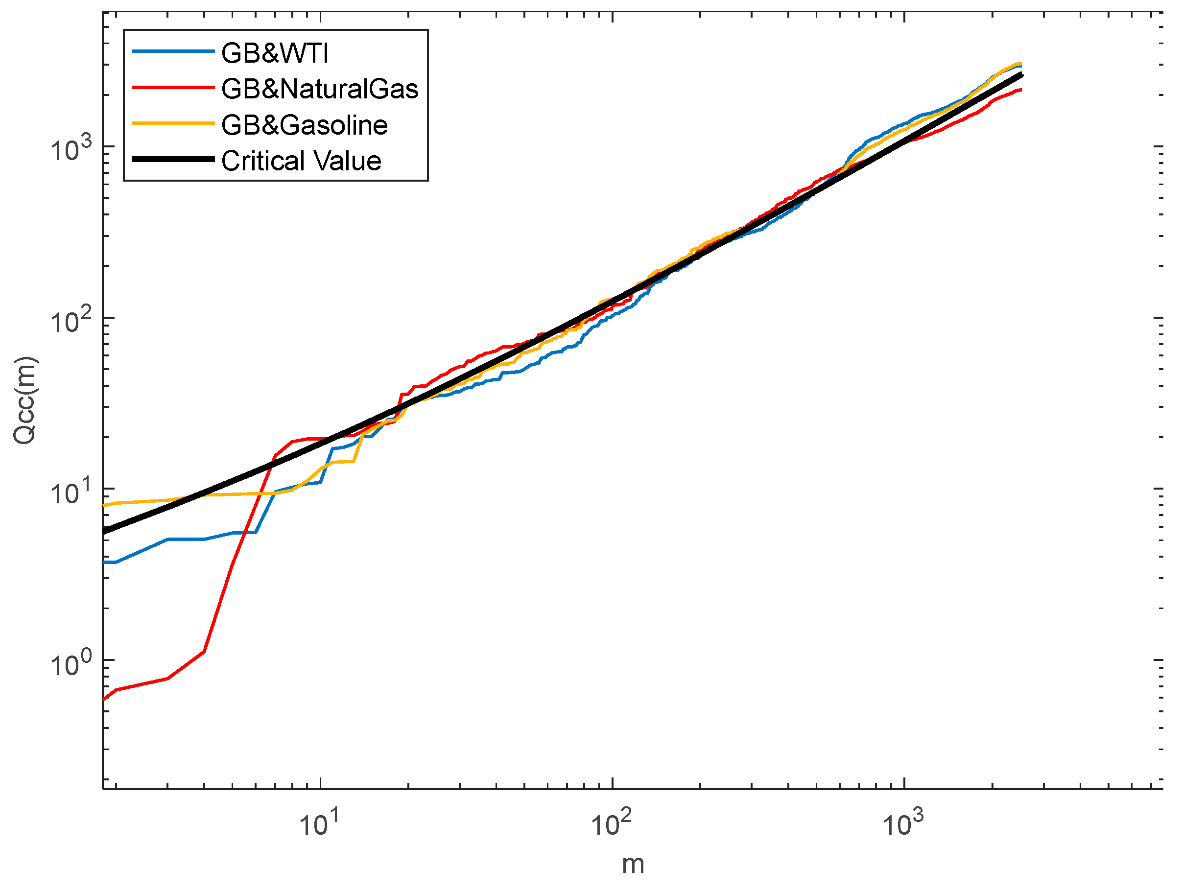
5.1. Cross-Correlation Test

Podobnik et al. [36] proposed cross-correlation test to analyze the nonlinear cross-correlation between two time series. Assuming that the time series $x_i$ and $y_i$ (i = 1, 2, …, N) are statistically independent, the statistic is calculated as follows:

$$Q_{cc}\left(m\right)=N^2\sum _{i=1}^m{\displaystyle \frac{A_i^2}{N-i}}$$

(31)

where N denotes the sample sequence length, while $A_i$ represents the cross-correlation function of the two sequences.

$${\mathrm{A}}_{\mathrm{i}}={\displaystyle \frac{{\sum }_{\mathrm{k}=\mathrm{i}+1}^{\mathrm{N}}{\mathrm{x}}_{\mathrm{k}}{\mathrm{y}}_{\mathrm{k}-\mathrm{i}}}{\sqrt{{\sum }_{\mathrm{k}=1}^{\mathrm{N}}{\mathrm{x}}_{\mathrm{k}}^2{\sum }_{\mathrm{k}=1}^{\mathrm{N}}{\mathrm{y}}_{\mathrm{k}}^2}}}$$

(32)

The test’s null hypothesis is that the $Q_{cc}\left(m\right)$ statistic approximately follows a ${\chi }^2\left(m\right)$ distribution, indicating the absence of cross-correlation between the two time series. However, when the test statistics significantly deviate from the critical value of the ${\chi }^2$ distribution at a given confidence level, it suggests the existence of cross-correlation.

Figure 2 displayed the Q_cc (m) statistics between the Green Bond and three energy futures across different degrees of freedom m. Both the statistics and the degrees of freedom m were shown on a logarithmic scale, with the 95% confidence level critical value of the ${\chi }^2\left(m\right)$ indicated by a bold black solid line. It was evident that the statistics significantly deviated from the critical value at both small and large m. This indicated the presence of nonlinear cross-correlations between the Green Bond and three energy futures.

Zebende [37] introduced the DCCA coefficient ${\rho }_{DCCA}$ to further quantify the level of cross-correlation. The DCCA coefficient is primarily expressed as the detrended covariance function of the sequences {$x_t$} and {$y_t$} divided by the product of the detrended variance functions of the two sequences.

$${\mathit{\rho }}_{\mathit{D}\mathit{C}\mathit{C}\mathit{A}}\mathit{=}\frac{{\mathit{F}}_{\mathit{D}\mathit{C}\mathit{C}\mathit{A}}^{\mathit{2}}\left(\mathit{x}\mathit{y}\mathit{,}\mathit{s}\right)}{{\mathit{F}}_{\mathit{D}\mathit{F}\mathit{A}}\left(\mathit{x}\mathit{,}\mathit{s}\right){\mathit{F}}_{\mathit{D}\mathit{F}\mathit{A}}\left(\mathit{y}\mathit{,}\mathit{s}\right)}$$

(33)

The coefficient ${\rho }_{DCCA}$ ranges from −1 to 1. The value of ${\rho }_{DCCA}$ equals to 1 or −1, indicating a perfect cross-correlation or perfect anti-cross-correlation between the two time series, respectively. The coefficient of 0 signifies that there is no cross-correlation between the sequences.

Figure 3 illustrated the coefficient results between the Green Bond and energy futures across different time scales s. It was observed that all coefficients were negative, indicating negative cross-correlations. Furthermore, as the scale s increased, the absolute value of the DCCA coefficients also increased, suggesting that the negative cross-correlations between the Green Bond and these energy futures became more pronounced. Additionally, the DCCA coefficient between Green Bond and natural gas consistently remained the smallest, while the DCCA coefficients for the other two series became more similar as s increased. This cross-correlation test could only detect the presence of cross-correlations and could not confirm persistence or anti-persistence. Therefore, further analysis using multifractal methods was required.

5.2. Skewed Multifractal Detrended Fluctuation Analysis

This study focuses on a sample period that includes major external shocks, notably the COVID-19 pandemic and the Russia–Ukraine war. Prior research has shown that both events significantly affected the multifractal characteristics of Green Bond and energy futures markets [38,39]. Therefore, to examine whether these shocks triggered structural breaks and altered multifractal cross-correlations, this study employs the skewed MF-DCCA method.

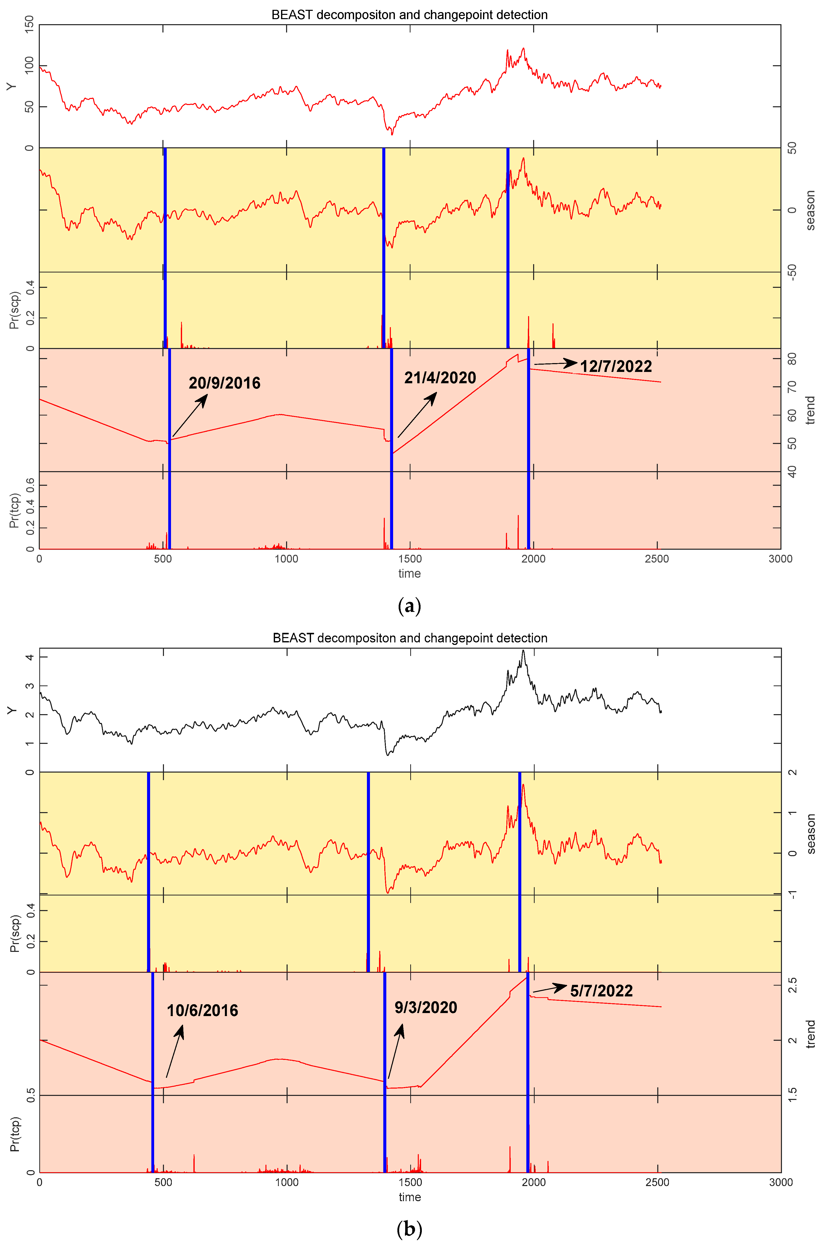
5.2.1. Results and Analysis of Change Point Identification

The dataset used in this study ranges from 1 August 2014 to 28 August 2024, which includes international events such as the European energy crisis, the COVID-19 pandemic, and the Russia–Ukraine war. To identify change points, this section will employ the BEAST method which can be carried out utilizing the MATLAB R2022a code package accessible on the website.

Figure 4 presented the change point identification results of the Green Bond and three energy futures. It was observed that multiple change points were detected in the nexuses between Green Bond and these three energy futures.

It was observed that the nexus between the Green Bond and WTI crude oil experienced abrupt changes at the following points: $X_1$ on 20 September 2016, $X_2$ on 21 April 2020, and $X_3$ on 12 July 2022. In comparison, the nexus between Green Bond and gasoline experienced shifts at the following points: $X_1$ on 10 June 2016, $X_2$ on 9 March 2020, and $X_3$ on 5 July 2022. This indicated that both the Green Bond and WTI group and the Green Bond and Gasoline group exhibited three significant change points. However, the nexus between Green Bond and natural gas experienced shifts at only two change points: $X_1$ on 23 September 2020, and $X_2$ on 15 September 2022.

We compared the dates on which these change points occurred by aligning them with relevant external factors and the broader historical context. These observations suggest a strong link to exogenous shocks. First, we explored the similarity and formation mechanisms of the structural changes in the Green Bond and WTI and Green Bond and Gasoline groups. We found that the $X_2$ and $X_3$ change points in both groups are almost aligned in time, primarily due to the simultaneous impact of major economic events and the tight interconnection between energy futures markets. Specifically, WTI crude oil futures and RBOB gasoline futures are highly correlated energy products [40] and typically exhibit synchronous movements during periods of intense market turbulence. For example, in the $X_2$ phase, the COVID-19 outbreak caused a steep drop in global energy demand and severe oil-market turmoil. At the same time, green stimulus policies worldwide buoyed investor sentiment and redirected capital into Green Bond. This dual effect induced pronounced structural shifts in both group correlations simultaneously. In the $X_3$ phase, the Russia–Ukraine conflict prompted European energy sanctions and sent crude oil and gasoline prices soaring; combined with a surge in global sustainable investment demand, this further drove coordinated adjustments in both groups’ correlations under the energy-crisis backdrop. By contrast, the timing discrepancy of the $X_1$ change points between these two groups reflects the asynchronous influence of distinct external events: the WTI market was hit by Gulf of Mexico hurricanes, which triggered sudden inventory drawdowns compounded by OPEC production-cut expectations, while Green Bond expanded and attracted safe-haven flows; meanwhile, the gasoline futures market was propelled by seasonal demand shifts, whose price rebound enhanced the appeal of fossil-fuel investments. This misalignment of event chronologies led to asynchronous structural breaks in the two group correlations.

Second, we examined why the change points in the Green Bond and Natural Gas group differ from those observed in the first two groups. Several factors may explain this: At $X_1$, the global economy was gradually recovering from the initial impact of the COVID-19 pandemic. Both the Green Bond and natural gas futures markets were influenced by this rebound in energy demand and the growing wave of green investments. At $X_2$, the outbreak of the Russia–Ukraine war led to a surge in global natural gas prices. In response, global demand for and investment in renewable energy accelerated, benefiting the Green Bond market. It can be observed that similar to the previous two groups, the two change points in the Green Bond and Natural Gas group were also dominated by macro factors, reflecting the common influence of international events on energy markets. However, unlike the previous two groups, this group only exhibited two significant change points. This phenomenon is not surprising, as the $X_1$ change points in the first two groups were driven by various external events experienced by the energy futures markets, which are market-specific and distinctive. Moreover, prior to 2020, due to market sentiment, economic data, and other macro factors, the correlation between Green Bond and natural gas prices was relatively low and even insignificant [38]. It suggested that during this period, there was a lack of clear linkage effect between the Green Bond and natural gas markets, and the nexus between them did not exhibit significant fluctuations. This further clarifies why this group has fewer change points.

These change points were all detected using the BEAST algorithm. It can be concluded that the BEAST algorithm not only successfully detects significant international events such as the COVID-19 pandemic and the Russia–Ukraine war but also captures external events like OPEC’s discussions on production cut agreements, demonstrating its accuracy.

So, how do we make a selection from so many change points? By examining Figure 4a–c as a whole, it became clear that these three groups of nexuses experienced change points at specific times, driven by either market-specific factors or macroeconomic factors. After careful consideration, we decided to focus on the change points influenced by macroeconomic events, while excluding those caused by market-specific factors. There were two main reasons for this: First, structural changes caused by market-specific factors made the nexuses between the three groups no longer comparable, which limited the discussion. Second, previous studies have demonstrated that both the pandemic and war significantly impacted the spillover effects between the Green Bond and energy markets [6,7,41,42]. However, whether these events similarly affect the multifractal cross-correlations between the two markets remains an important research question. Exploring the differences and similarities in how these multifractal cross-correlations changed in response to macroeconomic events had practical significance, offering valuable insights for market participants. Consequently, in order to enhance the comparability and economic significance of this paper, this paper focuses solely on the change points related to the COVID-19 pandemic and the Russia–Ukraine war to further investigate the skewed multifractal characteristics of the cross-correlations between these sequences.

Table 2. The periods before and after the two change points. It should be noted that although the specific dates of the change points differ, they all reflect the impacts of the COVID-19 pandemic in 2020 and the Russia–Ukraine war in 2022 on the Green Bond and energy futures markets. Here, for clarity and simplicity, “Green Bond” has been abbreviated as “GB”.

	GB & WTI	GB & Gasoline	GB & Natural Gas
Period 1	1 August 2014 to 20 April 2020	1 August 2014 to 6 March 2020	1 August 2014 to 22 September 2020
Period 2	21 April 2020 to 11 July 2022	9 March 2020 to 1 July 2022	23 September 2020 to 14 September 2022
Period 3	12 July 2022 to 28 August 2024	5 July 2022 to 28 August 2024	15 September 2022 to 28 August 2024
Entire period	1 August 2014 to 28 August 2024	1 August 2014 to 28 August 2024	1 August 2014 to 28 August 2024

showed the intervals for the three sequence pairs derived from the detection results. For each group, two change points were selected and designated as change point 1 and change point 2. Notably, although change point 1 for each group occurred during the COVID-19 pandemic and change point 2 occurred during the Russia–Ukraine war, the specific timing of these points varied. This discrepancy can be attributed to the distinct characteristics of each energy futures market and their sensitivity to external changes.

During the pandemic, the sequence of change point 1 reflected the varying response speeds of different markets to the crisis. First, the global transportation lockdowns caused by the pandemic directly impacted gasoline price fluctuations [43], making the gasoline market the most responsive. Thus, its change point occurred first. Second, the WTI crude oil market was less directly impacted, with price fluctuations driven more by supply and demand dynamics [44] and investor behavior [45]. Although its response was slower than gasoline, the change point still appeared early in the pandemic. Lastly, the natural gas market adjusted more slowly due to its reliance on long-term contracts and infrastructure [46], resulting in the latest occurrence of change point 1.

During the Russia–Ukraine war, the sequence of change point 2 reflected the sensitivity of different markets to geopolitical conflicts and supply chain characteristics. Firstly, the change point for the gasoline group occurred earliest. As a daily consumer product, gasoline is highly sensitive to market dynamics, with geopolitical factors and supply constraints quickly driving up prices [47]. Secondly, the crude oil market reacted slightly slower due to the complexity of the global supply chain, including transportation, storage, and refining. Finally, the natural gas market exhibited the slowest reaction, with its change point occurring last, primarily due to the rigidity of its supply chain and long-term contracts [46].

Therefore, although the specific time points vary, we attribute change point 1 for each group to the COVID-19 pandemic and change point 2 to the Russia–Ukraine war. Based on these change points, the original time series was divided into three periods: Period 1, the phase before the first change point; Period 2, the phase between the first and second change points; and Period 3, the phase after the second change point. Consequently, Period 2 reflects the impact of the COVID-19 pandemic, while Period 3 captures the effect of the Russia–Ukraine war. To further validate the rationality of this segmentation approach and the accuracy of the detected change points, we conducted a robustness test in Section 5.4.

5.2.2. Skewed Multifractal Analysis

Then, we will investigate whether the multifractality of nexuses between Green Bond and the corresponding energy futures has changed before and after the selected change points. If changes are observed, it indicates that the change points have influenced the cross-correlations between the two sequences, suggesting the presence of skewed multifractality. This paper will subsequently apply the MF-DCCA method to the sub-intervals of each period. It is worth mentioning that, to compare the skewed MF-DCCA method with the traditional MF-DCCA approach, the result from the entire period based on the traditional MF-DCCA will be used as a benchmark for comparative analysis.

For the time scales, to ensure an adequate number of subintervals and to avoid excessive smoothing at large scales, this paper chose $s_{min}=10$ and $s_{max}={\displaystyle \frac{N}{5}}$. Also, the range of q selected in this study was $\mathrm{q}\in [-\mathrm{10,10}]$.

Figure 5 illustrated the fluctuation functions of the Green Bond and three energy futures across different time scales. As seen in Figure 5, fluctuation functions increased with rising s, indicating a positive slope and demonstrating a power-law relationship across all groups and periods.

Table 3. The scaling exponents of Green Bond and the three energy futures series with q values ranging from −10 to 10. Here, for clarity and simplicity, “natural gas” has been abbreviated as “NG”.

	Entire period			Period 1
q	GB&WTI	GB&Gasoline	GB&NG	GB&WTI	GB&Gasoline	GB&NG
−10	0.6800	0.6796	0.6784	0.5888	0.6105	0.6067
−8	0.6689	0.6677	0.6632	0.5803	0.6006	0.5958
−6	0.6551	0.6532	0.6434	0.5715	0.5897	0.5822
−4	0.6378	0.6351	0.6179	0.5638	0.5792	0.5655
−2	0.6119	0.6085	0.5873	0.5596	0.5696	0.5458
0	0.5650	0.5591	0.5624	0.5485	0.5482	0.5160
2	0.4940	0.4831	0.5519	0.4385	0.4844	0.4510
4	0.4130	0.3940	0.5162	0.2740	0.4128	0.3815
6	0.3573	0.3360	0.4813	0.1841	0.3638	0.3335
8	0.3232	0.3011	0.4563	0.1359	0.3319	0.3019
10	0.3010	0.2783	0.4386	0.1069	0.3104	0.2805
ΔH	0.3791	0.4012	0.2398	0.4818	0.3001	0.3262
	Period 2			Period 3
q	GB&WTI	GB&Gasoline	GB&NG	GB&WTI	GB&Gasoline	GB&NG
−10	0.7069	0.6441	0.7186	0.6173	0.6339	0.5913
−8	0.6968	0.6337	0.6976	0.6061	0.6240	0.5855
−6	0.6831	0.6202	0.6668	0.5900	0.6114	0.5797
−4	0.6632	0.6027	0.6227	0.5643	0.5943	0.5736
−2	0.6336	0.5827	0.5708	0.5177	0.5636	0.5609
0	0.6061	0.5808	0.5259	0.4398	0.4863	0.5145
2	0.5804	0.5770	0.4967	0.3615	0.3587	0.4361
4	0.5195	0.5269	0.4585	0.3130	0.2668	0.3793
6	0.4701	0.4876	0.4207	0.2804	0.2158	0.3432
8	0.4385	0.4620	0.3940	0.2568	0.1843	0.3183
10	0.4176	0.4446	0.3754	0.2393	0.1630	0.3003
ΔH	0.2893	0.1995	0.3432	0.3780	0.4709	0.2910

and Figure 6 displayed the generalized Hurst exponents corresponding to different q values between Green Bond and the three energy futures. It was observed that the generalized Hurst exponent decreased as q increased for all groups, indicating that the cross-correlations between Green Bond and three energy futures all exhibited multifractality. For $H\left(2\right)$, throughout the entire period, the Hurst exponents for Green Bond and WTI and Green Bond and Gasoline were less than 0.5, indicating anti-persistence. In contrast, the Green Bond and Natural Gas group exhibited persistence. In Period 1, all groups demonstrated anti-persistence. In Period 2, the Hurst exponents for all groups increased, with the Green Bond and WTI and Green Bond and Gasoline groups showing persistent characteristics, except for the Green Bond and Natural Gas group. In Period 3, the Hurst exponents for all groups decreased, indicating significant anti-persistence. For the $\mathsf{\Delta }H$, the value of the Green Bond and WTI and Green Bond and Gasoline groups decreased by 0.2577 and 0.1056, respectively, from Period 1 to Period 2. However, the Green Bond and Natural Gas group increased slightly by 0.0170. From Period 2 to Period 3, the $\mathsf{\Delta }H$ trends reversed. The Green Bond and WTI and Green Bond and Gasoline groups increased by 0.0887 and 0.2764, respectively, while Green Bond and Natural Gas decreased by 0.0522.

Figure 7 displayed the Renyi exponents versus q. It shows that as q varies, ${\tau }_{xy}\left(q\right)$ exhibited a nonlinear change, indicating that each pair of cross-correlations is multifractal. Figure 8a–c all presented upward concave shapes, with specific patterns varying across different periods. From the perspective of $\mathsf{\Delta }\alpha$, the results aligned with those of $\mathsf{\Delta }H$. It was observed that the $\mathsf{\Delta }\alpha$ for the Green Bond and WTI group and the Green Bond and Gasoline group decreased by 0.2594 and 0.1164, respectively, from period 1 to period 2, which indicated a reduction in multifractality. In contrast, the $\mathsf{\Delta }\alpha$ for the Green Bond and Natural Gas group increased by 0.0452 from period 1 to period 2, suggesting a more complex cross-correlation between Green Bond and natural gas futures. From period 2 to period 3, the $\mathsf{\Delta }\alpha$ values for the first two groups increased by 0.0803 and 0.2861, respectively, while the Green Bond and Natural Gas group decreased by 0.1140. It can be observed that the variation trend of $\mathsf{\Delta }\alpha$ is consistent with that of $\mathsf{\Delta }H$.

Table 4. The MRCC statistics between Green Bond and three energy futures for these periods. From top to bottom are the plots of ${\mathsf{\alpha }}_{\mathrm{x}\mathrm{y}}\left(0\right)$, ${\mathrm{W}}_{\mathrm{x}\mathrm{y}}$, and $\mathsf{\Gamma }$, respectively.

Cross Correlation	αxy (0)				Wxy				Γ
	Entire Period	Period I	Period II	Period III	Entire Period	Period I	Period II	Period III	Entire Period	Period I	Period II	Period III
GB&WTI	0.5619	0.5693	0.6078	0.4397	0.5171	0.6761	0.4167	0.4970	0.9203	1.1876	0.6856	1.1304
GB&Gasoline	0.5558	0.5420	0.5821	0.4784	0.5442	0.4311	0.3147	0.6008	0.9791	0.7954	0.5407	1.2559
GB&NG	0.5656	0.5107	0.5282	0.5096	0.3764	0.4599	0.5051	0.3911	0.6655	0.9006	0.9563	0.7675

illustrated the multifractal risk levels of cross-correlations for each group across different periods. The first section reported the ${\alpha }_{xy}\left(0\right)$ values. Except for the Green Bond and Gasoline and Green Bond and WTI groups in period 3, whose statistics were below 0.5 (indicating anti-persistence), all other values were above 0.5 (suggesting persistent cross-correlations). The second section displayed the $W_{xy}$ values, with the Green Bond and WTI group exhibiting the highest value in period 1, the Green Bond and Natural Gas group in period 2, and the Green Bond and Gasoline group in period 3. The third section presented the $\mathsf{\Gamma }$ values, which served as indicators of multifractal risk. Over the entire period, the Green Bond and Gasoline group recorded the highest value (0.9791), followed by the Green Bond and WTI group (0.9203) and the Green Bond and Natural Gas group (0.6655). For each period, from period 1 to period 2, the $\mathsf{\Gamma }$ values for the Green Bond and WTI and Green Bond and Gasoline groups decreased from 1.1876 and 0.7954 to 0.6856 and 0.5407, respectively, while the Green Bond and Natural Gas group increased from 0.9006 to 0.9563. From period 2 to period 3, the first two groups increased to 1.1304 and 1.2559, while the Green Bond and Natural Gas group decreased to 0.7675. It can be observed that the variation trend of $\mathsf{\Gamma }$ is consistent with that of $\mathsf{\Delta }H$ and $\mathsf{\Delta }\alpha$.

In summary, the values of ΔH, $\mathsf{\Delta }\alpha$, and $\mathsf{\Gamma }$, which represent multifractal intensity, exhibited a consistent pattern across groups. Specifically, both the GB and WTI and GB and Gasoline groups showed a decline followed by an increase during the COVID-19 period, while the GB and Natural Gas group displayed the opposite trend—an initial rise followed by a decline. This divergence can be explained as follows: During the COVID-19 pandemic, although the WTI crude oil and gasoline futures markets experienced severe shocks, the Green Bond market demonstrated notable resilience, which allowed it to serve as a hedge against oil price volatility [48]. This hedging effect partly weakened the multifractal cross-correlations between Green Bond and these two energy futures. In contrast, the natural gas market, constrained by long-term contracts and rigid infrastructure, adjusted at a slower pace [46]. This discrepancy in adjustment speeds led to a significant increase in the multifractal cross-correlations between Green Bond and natural gas after the pandemic outbreak. Additionally, the quantitative easing policies implemented during this period likely influenced the pricing mechanisms of energy futures and investor sentiment. This may have further strengthened the multifractal cross-correlations between Green Bond and natural gas futures [49]. In the subsequent period, spanning from the pandemic to the Russia–Ukraine war, the multifractal intensity between Green Bond and both WTI and gasoline markets increased, whereas the multifractal level between Green Bond and natural gas declined. This change was mainly driven by the differentiated impacts of the war on energy markets. The sanctions imposed on Russian energy imports by European countries led to a sharp rise in WTI and gasoline prices. At the same time, Green Bond, as an ESG-compliant investment instrument, attracted safe-haven capital, further reinforcing their nonlinear dependencies [25]. By contrast, the natural gas market exhibited a delayed response to supply and demand changes. Moreover, the war accelerated Europe’s energy transition and reduced its reliance on natural gas, which in turn weakened its short-term cross-correlation with the Green Bond market [46]. Overall, this skewed dynamic reflects the heterogeneous responses of different energy markets to external shocks and their complex interactions with the Green Bond market.

Moreover, compared to the traditional MF-DCCA method applied over the entire period, the skewed MF-DCCA approach proposed in this study revealed richer information about the dynamic evolution of multifractal cross-correlations. Regarding the Hurst exponent, the results from the entire period showed that the GB and WTI and GB and Gasoline groups exhibited anti-persistent behavior, while the GB and Natural Gas group showed persistent behavior. In contrast, the three sub-periods identified by the skewed method revealed notable temporal heterogeneity: during period 1, all groups displayed anti-persistent behavior; during period 2, the GB and WTI and GB and Gasoline groups shifted to persistence, whereas the GB and Natural Gas group exhibited anti-persistence, which was opposite to the finding from the entire period. During period 3, all groups consistently exhibited anti-persistent behavior. This evolution clearly illustrated the dynamic adjustment process of multifractal cross-correlations. Regarding ΔH, Δα, and Γ, the traditional MF-DCCA method over the entire period provided only static results. In contrast, the skewed MF-DCCA method, through time segmentation, demonstrated the dynamic evolution of multifractality and risk over time. Therefore, compared with the traditional MF-DCCA, the skewed approach not only overcame the limitation of ignoring structural breaks but also offered valuable insights into the dynamic multifractal behavior induced by such breaks, demonstrating significant methodological advantages.

5.3. Portfolio Management Implications

Some studies have shown that Green Bond exhibits safe-haven properties during heightened market uncertainty. For example, Huang et al. [5] found that Green Bond was negatively correlated with crude oil during the COVID-19 pandemic and the Russia–Ukraine conflict, highlighting their hedging potential. Other research [2,50] noted the generally low correlation between Green Bond and commodity markets, which supports their role in diversification and risk reduction.

Since the results of this study indicate that the COVID-19 pandemic and the Russia–Ukraine war intensified the multifractal risk between Green Bond and energy futures, it is necessary to examine further whether Green Bond effectively hedged the three major energy futures during these periods. In addition, to integrate multifractal characteristics into portfolio construction, this study employs the Mean-MF-DCCA model to build optimal portfolios. Their performance is then compared with that of conventional portfolio models.

Based on Equations (24)–(30), we construct eight portfolios: an energy-futures-only portfolio, an equal-weighted portfolio, a minimum-variance portfolio, a maximum Sharpe ratio portfolio, a minimum downside risk portfolio, and three portfolios generated by the Mean-MF-DCCA model (minimum-variance, maximum Sharpe ratio, and minimum downside risk). For each portfolio and across each period, we will calculate the optimal weights, expected return, expected variance, Sharpe ratio, and risk reduction effectiveness, and then compare their performance. The risk reduction effectiveness $\mathrm{R}\mathrm{R}\mathrm{E}$ of the portfolio is computed as follows:

$$\mathrm{R}\mathrm{R}\mathrm{E}=1-{\displaystyle \frac{{\mathrm{V}\mathrm{a}\mathrm{r}}_{\mathrm{p}ortfolio}}{{\mathrm{V}\mathrm{a}\mathrm{r}}_{\mathrm{e}nergyfutures}}}$$

(34)

where ${\mathrm{V}\mathrm{a}\mathrm{r}}_{\mathrm{p}ortfolio}$ is the variance of portfolio, and ${\mathrm{V}\mathrm{a}\mathrm{r}}_{\mathrm{e}nergyfutures}$ is the variance of the energy-futures-only portfolio. A higher RRE value signifies a better risk reduction effectiveness.

Table 5. Performance of different portfolios across various periods. The rows report the portfolio weights for Green Bond and different energy futures, Sharpe ratio (SR) and risk reduction effectiveness (RRE), all in %. The columns present eight portfolio models constructed for each period: an energy-futures-only portfolio, an equal-weighted portfolio, a minimum-variance (MV) portfolio, a maximum Sharpe ratio (MaxSR) portfolio, a minimum downside risk (MD) portfolio, and three portfolios generated by the Mean-MF-DCCA model (Mean-MF-DCCA MV, Mean-MF-DCCA MaxSR, and Mean-MF-DCCA MD).

Period	Portfolios	Weight: GB/WTI	SR	RRE	Weight: GB/Gasoline	SR	RRE	Weight: GB/NG	SR	RRE
Period 1	energy only	0/100	−4.13	-	0/100	−3.37	-	0/100	−2.13	-
	equal weighted	50/50	−4.69	49.81	50/50	−3.84	49.72	50/50	−2.49	49.61
	MV	98.46/1.54	−5.60	88.70	98.37/1.63	−4.43	87.93	98.86/1.14	−3.55	88.69
	MaxSR	0/100	−4.13	0.00	0/100	−3.37	0.00	0/100	−2.13	0.00
	MD	99.04/0.96	−5.41	88.69	98.47/1.53	−4.40	87.93	99.07/0.93	−3.52	88.69
	Mean-MF-DCCA MV	97.27/2.73	−0.80	92.79	98.34/1.66	−1.17	91.03	94.31/5.69	0.12	91.86
	Mean-MF-DCCA MaxSR	100/0	−0.90	92.50	0/100	5.12	86.10	100/0	−0.15	91.62
	Mean-MF-DCCA MD	99.04/0.96	−0.84	92.69	98.89/1.11	−1.11	91.01	94.91/5.09	−0.12	91.65
Period 2	energy only	0/100	7.12	-	0/100	3.66	-	0/100	6.65	-
	equal weighted	50/50	5.92	49.54	50/50	2.30	49.29	50/50	5.25	49.88
	MV	99.5/0.5	−11.24	90.24	99.6/0.4	−11.85	88.97	99.15/0.85	−15.61	91.50
	MaxSR	0/100	7.12	0.00	0/100	3.66	0.00	0/100	6.65	0.00
	MD	98.9/1.1	−10.71	90.22	99.65/0.35	−11.87	88.97	98.61/1.39	−15.07	91.49
	Mean-MF-DCCA MV	98.4/1.6	−0.50	90.19	92.33/7.67	−1.67	92.14	96.54/3.46	−0.03	92.07
	Mean-MF-DCCA MaxSR	100/0	−0.54	90.05	0/100	2.90	87.38	100/0	−0.26	91.86
	Mean-MF-DCCA MD	98.46/1.54	−0.54	90.06	99.65/0.35	−1.18	92.01	96.84/3.16	−0.24	91.88
Period 3	energy only	0/100	−3.85	-	0/100	−5.41	-	0/100	−7.16	-
	equal weighted	50/50	−3.63	48.32	50/50	−5.28	48.56	50/50	1.10	49.40
	MV	94.38/5.62	−0.50	75.69	95.39/4.61	−1.23	77.78	99.34/0.66	1.53	88.85
	MaxSR	100/0	0.40	75.01	100/0	−0.11	77.29	100/0	−6.91	88.84
	MD	94.94/5.06	−0.41	75.68	96.87/3.13	−0.87	77.73	99.66/0.34	1.31	88.85
	Mean-MF-DCCA MV	96.84/3.16	−0.44	91.38	94.99/5.01	−2.29	94.39	96.3/3.7	0.52	96.71
	Mean-MF-DCCA MaxSR	100/0	−0.50	91.24	0/100	8.09	91.78	100/0	−0.28	96.44
	Mean-MF-DCCA MD	99.07/0.93	−0.46	91.34	98.61/1.39	−1.75	94.34	99.63/0.37	0.44	96.69

presented the performance of different portfolio types across various periods. All portfolios exhibited positive RRE in every period, indicating that Green Bond served as an effective hedge against energy futures. Specifically, the equal-weighted portfolio consistently showed the lowest RRE values. In contrast, the portfolios constructed using the Mean-MF-DCCA model achieved the highest RRE values, significantly higher than those of the traditional minimum-variance, maximum Sharpe ratio, and minimum downside risk portfolios. This demonstrated that portfolios constructed with the Mean-MF-DCCA model incorporated multifractal features achieved superior risk reduction, even during crisis periods. As for the Sharpe ratio, the best-performing portfolios were mostly those constructed using the Mean-MF-DCCA model, with only four exceptions where the traditional maximum Sharpe ratio or minimum-variance portfolios outperformed. This suggests investors can rely on the Mean-MF-DCCA model portfolios to optimize risk-adjusted returns.

Overall, investors are advised to include Green Bond in their portfolios as an effective hedge against energy futures risk, especially during crisis periods. Concurrently, they should account for multifractal risks and prioritize portfolio construction using the Mean-MF-DCCA model to achieve an optimal balance between risk and return.

5.4. Robustness Check of Change Points

Our change points were identified using the BEAST method. To explore the economic significance of these change points, we matched their occurrence dates with major external events. As a result, Change Point 1 was interpreted as corresponding to the structural shifts caused by the COVID-19 pandemic, while Change Point 2 was associated with the outbreak of the Russia–Ukraine war. Accordingly, the original time series was divided into three distinct periods.

We conducted a robustness check to validate the accuracy of the identified change points and the relevance of their associated economic interpretations. Drawing on the classifications commonly used in existing literature [24,26], the period before the COVID-19 pandemic is typically defined as the stage before 10 March 2020; the pandemic period as spanning from 11 March 2020 to 23 February 2022; and the Russia–Ukraine war period as the stage after 24 February 2022. Based on this, we constructed an alternative sequence segmented strictly according to these economic events and compared it with our sequence segmented using the BEAST method. This comparison aimed to evaluate whether the skewed multifractal features identified under both segmentations yielded consistent results.

As shown, regarding the Hurst exponent H(2), both segm in

Table 6. Robustness check of change points: Here, period 1 corresponds to the pre-pandemic stage, period 2 represents the pandemic and pre-war stage, and period 3 covers the post-war period. The BEAST-identified sequence refers to the segmentation derived from the BEAST method, while the economic event sequence is based on event-driven segmentation drawn from established literature [24,26].

Multifractal Indicator	Period	Group	BEAST-Identified Sequence	Economic Event Sequence
Hurst exponent	1	GB&WTI	0.4361	0.3941
		GB&Gasoline	0.4844	0.4711
		GB&NG	0.4510	0.4615
	2	GB&WTI	0.5804	0.5138
		GB&Gasoline	0.6097	0.5227
		GB&NG	0.4967	0.4017
	3	GB&WTI	0.3615	0.3031
		GB&Gasoline	0.3587	0.4520
		GB&NG	0.4361	0.4768
ΔH	1	GB&WTI	0.5471	0.4650
		GB&Gasoline	0.3001	0.3341
		GB&NG	0.3262	0.3168
	2	GB&WTI	0.2893	0.3891
		GB&Gasoline	0.1945	0.2629
		GB&NG	0.3432	0.3971
	3	GB&WTI	0.3780	0.5952
		GB&Gasoline	0.4709	0.3053
		GB&NG	0.2910	0.2675
Wxy	1	GB&WTI	0.6761	0.6043
		GB&Gasoline	0.4167	0.4770
		GB&NG	0.4970	0.4568
	2	GB&WTI	0.4311	0.5442
		GB&Gasoline	0.3147	0.3968
		GB&NG	0.6008	0.5449
	3	GB&WTI	0.4599	0.7522
		GB&Gasoline	0.5051	0.4175
		GB&NG	0.3911	0.3594
Γ	1	GB&WTI	1.1876	1.2047
		GB&Gasoline	0.6856	0.7925
		GB&NG	1.1304	0.8178
	2	GB&WTI	0.7954	0.9572
		GB&Gasoline	0.5407	0.7547
		GB&NG	1.2559	0.8898
	3	GB&WTI	0.9006	1.6849
		GB&Gasoline	0.9563	0.8023
		GB&NG	0.7675	0.7560

entation approaches indicated that all three pairs exhibit anti-persistent multifractal cross-correlation characteristics in period 1. In period 2, both segmentation methods showed that the GB and WTI and GB and Gasoline groups exhibit persistence, while the GB and Natural Gas group displayed anti-persistence. In period 3, all groups consistently exhibit anti-persistent behavior.

For ΔH, the multifractal spectrum width Wxy and the multifractal risk level Γ, although there are slight differences in the specific values, both segmentation methods consistently show that the multifractality of the GB and WTI and GB and Gasoline groups followed a pattern of initial decline followed by an increase. Conversely, the GB and Natural Gas pair showed an increasing trend followed by decreasing multifractality. These consistent results confirm the robustness of our change point detection method and the validity of its associated economic interpretations. The slight differences in the exact timing of the change points may reflect the lagged effects of the COVID-19 pandemic and the Russia–Ukraine war on the Green Bond and energy futures markets.

6. Conclusions

This study employed the skewed MF-DCCA method to investigate the asymmetric multifractal cross-correlations between Green Bond and major energy futures. First, this study employed the BEAST algorithm to identify structural change points and found that the nexus between Green Bond and energy futures exhibited significant common change points around key events, such as the outbreak of the COVID-19 pandemic and the onset of the Russia–Ukraine War. Robustness tests further confirmed that these events substantially impacted the relationship between Green Bond and energy futures. Based on the identified change points, the sample was segmented into three distinct periods: the pre-pandemic period, the pandemic period before the war, and the war period. The MF-DCCA method was applied to the entire period and each sub-period separately. The empirical findings demonstrated that the multifractal cross-correlations between Green Bond and energy futures varied considerably across these periods, revealing distinct skewed multifractal characteristics. Specifically, from the pre-pandemic period to the war period, the GB and WTI and GB and Gasoline groups exhibited a decline in multifractality followed by an upward shift, whereas the GB and Natural Gas group displayed the opposite trend, with an initial increase and a subsequent decrease. Moreover, a comparison with the conventional MF-DCCA method applied over the entire period showed that the proposed skewed MF-DCCA approach could capture more detailed insights into the dynamic evolution of multifractal cross-correlations, highlighting its methodological advantage. To enhance the practical relevance of the findings, the Mean MF-DCCA portfolio model was introduced to assess the hedging effectiveness of Green Bond against energy futures across different periods. The results confirmed that Green Bond effectively hedged against energy futures, particularly during crisis periods. Moreover, portfolios constructed using the Mean MF-DCCA framework, which incorporates multifractal characteristics, exhibited superior risk-adjusted performance compared to those constructed by conventional models.

These findings are generally consistent with existing literature. Fernandes and Acikgoz et al. [23,25] employed the MF-DCCA method and revealed significant multifractal cross-correlations between Green Bond and various financial assets, including energy commodities, which aligns well with our results from the entire period. However, compared with previous studies that focused on Green Bond and broad energy categories or indices, this research offers a more granular examination by investigating the multifractal cross-correlations between Green Bond and several specific energy futures. Moreover, it introduces methodological improvements by providing more comprehensive skewed multifractal results based on identified change points. In addition, Kojic, Inacio, and Adekoya et al. [24,26,27] empirically demonstrated the impact of the COVID-19 pandemic and the Russia–Ukraine conflict on the multifractal cross-correlations between Green Bond and conventional bonds, among different energy futures, as well as between energy futures and equity markets, which provides further support for this study. However, unlike the studies that primarily relied on empirical or subjectively defined sample periods, this study innovatively introduced the BEAST method to detect trend change points and segment the time series based on these points. This approach not only captures the lagged effects of significant events on market structure but also enhances the statistical significance and accuracy of segmentation. Finally, consistent with Huang et al. [5], this study confirmed Green Bond’s hedging effectiveness against various energy futures. However, this paper constructed investment portfolios with better performance than traditional models by using the Mean-MF-DCCA method that incorporates multifractal characteristics.

The findings of this study offer important practical implications for risk management and portfolio construction. Identifying structural change points linked to major external shocks highlights investors’ need to adjust asset allocations in response to evolving market conditions dynamically. The analysis confirms that Green Bond can be an effective hedging instrument against energy futures, especially during periods of heightened market uncertainty, such as global crises. Furthermore, applying the Mean MF-DCCA portfolio model demonstrates that incorporating multifractal characteristics into portfolio design can substantially improve risk-adjusted returns compared to traditional strategies. These insights can assist market participants in enhancing diversification, optimizing hedging strategies, and strengthening portfolio resilience in the face of complex market dynamics. For policymakers and regulators, this study suggests developing cross-market monitoring tools, such as a “Cross-Market Fractal Coupling Index”, and integrating multifractal risks into policy frameworks. Encouraging the inclusion of Green Bond in energy portfolios—through mechanisms like tax incentives—could also help enhance market stability. Lastly, regulators should work towards improving transparency and real-time oversight by incorporating multifractal risk indicators into their monitoring systems, thereby strengthening their capacity to manage systemic risks during global crises. These measures can support more robust market governance in response to evolving dynamics and external shocks.

Given that the S&P Green Bond Index was established in 2014, the available data for Green Bond are considerably shorter than that for energy futures. To ensure consistency in sample length, this study was limited to a reduced time span, which may have led to the omission of certain periods. Future research could extend the data range for a more comprehensive examination of the multifractal cross-correlations between Green Bond and energy futures. Furthermore, the skewed MF-DCCA method mainly emphasizes the internal complexity of cross-correlations. Future studies could incorporate external factors such as monetary policy, inflation, and investor sentiment to conduct a more in-depth investigation. Additionally, adopting alternative econometric models, expanding the analysis to include more financial assets, or conducting cross-market comparisons would help validate the robustness of the findings under different economic conditions.

References

1. Weckroth, M.; Ala-Mantila, S. Socioeconomic geography of climate change views in Europe. Glob. Environ. Change-Hum. Policy Dimens. 2022, 72, 102453. [Google Scholar] [CrossRef]
2. Arif, M.; Naeem, M.A.; Farid, S.; Nepal, R.; Jamasb, T. Diversifier or more? Hedge and safe haven properties of green bonds during COVID-19. Energy Policy 2022, 168, 113102. [Google Scholar] [CrossRef]
3. Naeem, M.A.; Bouri, E.; Costa, M.D.; Naifar, N.; Shahzad, S.J.H. Energy markets and green bonds: A tail dependence analysis with time-varying optimal copulas and portfolio implications. Resour. Policy 2021, 74, 102418. [Google Scholar] [CrossRef]
4. Naeem, M.A.; Nguyen, T.T.H.; Nepal, R.; Ngo, Q.-T.; Taghizadeh–Hesary, F. Asymmetric relationship between green bonds and commodities: Evidence from extreme quantile approach. Financ. Res. Lett. 2021, 43, 101983. [Google Scholar] [CrossRef]
5. Huang, J.; Cao, Y.; Zhong, P. Searching for a safe haven to crude oil: Green bond or precious metals? Financ. Res. Lett. 2022, 50, 103303. [Google Scholar] [CrossRef]
6. Dai, Z.; Zhang, X.; Yin, Z. Extreme time-varying spillovers between high carbon emission stocks, green bond and crude oil: Evidence from a quantile-based analysis. Energy Econ. 2023, 118, 106511. [Google Scholar] [CrossRef]
7. Ren, X.; Xiao, Y.; Kun, D.; Urquhart, A. Spillover effects between fossil energy and green markets: Evidence from informational inefficiency. Energy Econ. 2024, 131, 107317. [Google Scholar] [CrossRef]
8. Lucey, B.; Ren, B. Time-varying tail risk connectedness among sustainability-related products and fossil energy investments. Energy Econ. 2023, 126, 106812. [Google Scholar] [CrossRef]
9. Li, Z.; Tian, Y. Skewed multifractal cross-correlation between price and volume during the COVID-19 pandemic: Evidence from China and European carbon markets. Appl. Energy 2024, 371, 123716. [Google Scholar] [CrossRef]
10. Fama, E.F. Efficient Capital Markets: A Review of Theory and Empirical Work. J. Financ. 1970, 25, 383–417. [Google Scholar] [CrossRef]
11. Mantegna, R.N.; Stanley, H.E. Stock market dynamics and turbulence: Parallel analysis of fluctuation phenomena. Phys. A Stat. Mech. Its Appl. 1997, 239, 255–266. [Google Scholar] [CrossRef]
12. Yuan, Y.; Zhuang, X.-T.; Liu, Z.-Y.; Huang, W.-Q. Time-clustering behavior of sharp fluctuation sequences in Chinese stock markets. Chaos Solitons Fractals 2012, 45, 838–845. [Google Scholar] [CrossRef]
13. Peng, C.K.; Buldyrev, S.V.; Havlin, S.; Simons, M.; Stanley, H.E.; Goldberger, A.L. Mosaic organization of DNA nucleotides. Phys. Rev. E 1994, 49, 1685–1689. [Google Scholar] [CrossRef]
14. Podobnik, B.; Stanley, H.E. Detrended cross-correlation analysis: A new method for analyzing two nonstationary time series. Phys. Rev. Lett. 2008, 100, 084102. [Google Scholar] [CrossRef]
15. Kantelhardt, J.W.; Zschiegner, S.A.; Koscielny-Bunde, E.; Havlin, S.; Bunde, A.; Stanley, H.E. Multifractal detrended fluctuation analysis of nonstationary time series. Phys. A Stat. Mech. Its Appl. 2002, 316, 87–114. [Google Scholar] [CrossRef]
16. dos Santos Maciel, L. Brazilian stock-market efficiency before and after COVID-19: The roles of fractality and predictability. Glob. Financ. J. 2023, 58, 100887. [Google Scholar] [CrossRef]
17. Telli, S.; Chen, H.Z. Multifractal behavior in return and volatility series of Bitcoin and gold in comparison. Chaos Solitons Fractals 2020, 139, 109994. [Google Scholar] [CrossRef]
18. Gu, R.B.; Liu, S.N. Nonlinear analysis of economic policy uncertainty: Based on the data in China, the US and the global. Phys. A Stat. Mech. Its Appl. 2022, 593, 126897. [Google Scholar] [CrossRef]
19. Zhou, W.X. Multifractal detrended cross-correlation analysis for two nonstationary signals. Phys. Rev. E 2008, 77, 066211. [Google Scholar] [CrossRef]
20. Li, Z.; Lu, X. Cross-correlations between agricultural commodity futures markets in the US and China. Phys. A Stat. Mech. Its Appl. 2012, 391, 3930–3941. [Google Scholar] [CrossRef]
21. Fernandes, L.H.S.; Silva, J.W.L.; de Araujo, F.H.A. Multifractal risk measures by Macroeconophysics perspective: The case of Brazilian inflation dynamics. Chaos Solitons Fractals 2022, 158, 112052. [Google Scholar] [CrossRef]
22. Feng, Y.; Yang, J.; Huang, Q. Multiscale correlation analysis of Sino-US corn futures markets and the impact of international crude oil price: A new perspective from the multifractal method. Financ. Res. Lett. 2023, 53, 103691. [Google Scholar] [CrossRef]
23. Fernandes, L.H.S.; Silva, J.W.L.; de Araujo, F.H.A.; Tabak, B.M. Multifractal cross-correlations between green bonds and financial assets. Financ. Res. Lett. 2023, 53, 103603. [Google Scholar] [CrossRef]
24. Inacio, C.M.C.; Kristoufek, L.; David, S.A. Dynamic price interactions in energy commodities benchmarks: Insights from multifractal analysis during crisis periods. Phys. A Stat. Mech. Its Appl. 2025, 659, 130314. [Google Scholar] [CrossRef]
25. Acikgoz, T.; Gokten, S.; Soylu, A.B. Multifractal Detrended Cross-Correlations between Green Bonds and Commodity Markets: An Exploration of the Complex Connections between Green Finance and Commodities from the Econophysics Perspective. Fractal Fract. 2024, 8, 117. [Google Scholar] [CrossRef]
26. Kojic, M.; Mitic, P.; Schlueter, S.; Rakic, S. Complex non-linear relationship between conventional and green bonds: Insights amidst COVID-19 and the RU-UA conflict. J. Behav. Exp. Financ. 2024, 43, 100966. [Google Scholar] [CrossRef]
27. Adekoya, O.B.; Asl, M.G.; Oliyide, J.A.; Izadi, P. Multifractality and cross-correlation between the crude oil and the European and non-European stock markets during the Russia-Ukraine war. Resour. Policy 2023, 80, 103134. [Google Scholar] [CrossRef]
28. Saâdaoui, F. Skewed multifractal scaling of stock markets during the COVID-19 pandemic. Chaos Solitons Fractals 2023, 170, 113372. [Google Scholar] [CrossRef]
29. Saâdaoui, F. Segmented multifractal detrended fluctuation analysis for assessing inefficiency in North African stock markets. Chaos Solitons Fractals 2024, 181, 114652. [Google Scholar] [CrossRef]
30. Zhaoa, K.G.; Wulder, M.A.; Hu, T.X.; Bright, R.; Wu, Q.S.; Qin, H.M.; Li, Y.; Toman, E.; Mallick, B.; Zhang, X.; et al. Detecting change-point, trend, and seasonality in satellite time series data to track abrupt changes and nonlinear dynamics: A Bayesian ensemble algorithm. Remote Sens. Environ. 2019, 232, 111181. [Google Scholar] [CrossRef]
31. Wang, L.; Fu, A.; Bashir, B.; Gu, J.; Sheng, H.; Deng, L.; Deng, W.; Alsafadi, K. Characteristics and Driving Mechanisms of Coastal Wind Speed during the Typhoon Season: A Case Study of Typhoon Lekima. Atmosphere 2024, 15, 880. [Google Scholar] [CrossRef]
32. Yang, L.; Wang, C.; Zhou, P.; Xie, N.; Tian, M.; Wang, K. Change point detection in brucellosis time series from 2010 to 2023 in Xinjiang China using the BEAST algorithm. Sci. Rep. 2025, 15, 3830. [Google Scholar] [CrossRef]
33. Jewell, S.; Fearnhead, P.; Witten, D. Testing for a Change in Mean After Changepoint Detection. J. R. Stat. Soc. Ser. B Stat. Methodol. 2022, 84, 1082–1104. [Google Scholar] [CrossRef]
34. Piotr, F. Wild binary segmentation for multiple change-point detection. Ann. Stat. 2014, 42, 2243–2281. [Google Scholar] [CrossRef]
35. Li, J.; Wu, X.; Zhang, L.; Feng, Q. Research on the portfolio model based on Mean-MF-DCCA under multifractal feature constraint. J. Comput. Appl. Math. 2021, 386, 113264. [Google Scholar] [CrossRef]
36. Podobnik, B.; Grosse, I.; Horvatic, D.; Ilic, S.; Ivanov, P.C.; Stanley, H.E. Quantifying cross-correlations using local and global detrending approaches. Eur. Phys. J. B 2009, 71, 243–250. [Google Scholar] [CrossRef]
37. Zebende, G.F. DCCA cross-correlation coefficient: Quantifying level of cross-correlation. Phys. A Stat. Mech. Its Appl. 2011, 390, 614–618. [Google Scholar] [CrossRef]
38. Xiang, S.; Cao, Y. Green finance and natural resources commodities prices: Evidence from COVID-19 period. Resour. Policy 2023, 80, 103200. [Google Scholar] [CrossRef]
39. Wei, J.-W.; Wang, H.-Y.; Cao, G.-X. Multifractal Analysis of International Energy and Agricultural Markets Under the Influence of Russia-Ukraine Conflict. Fluct. Noise Lett. 2024, 23, 2450034. [Google Scholar] [CrossRef]
40. Vides, J.C.; Feria, J.; Golpe, A.A.; Martín-Álvarez, J.M. How do supply or demand shocks affect the US oil market? Financ. Innov. 2024, 10, 16. [Google Scholar] [CrossRef]
41. Mensi, W.; Selmi, R.; Al-Kharusi, S.; Belghouthi, H.E.; Kang, S.H. Connectedness between green bonds, conventional bonds, oil, heating oil, natural gas, and petrol: New evidence during bear and bull market scenarios. Resour. Policy 2024, 91, 104888. [Google Scholar] [CrossRef]
42. Mensi, W.; Vo, X.V.; Ko, H.-U.; Kang, S.H. Frequency spillovers between green bonds, global factors and stock market before and during COVID-19 crisis. Econ. Anal. Policy 2023, 77, 558–580. [Google Scholar] [CrossRef]
43. Patino-Artaza, H.; King, L.C.; Savin, I. Did COVID-19 really change our lifestyles? Evidence from transport energy consumption in Europe. Energy Policy 2024, 191, 114204. [Google Scholar] [CrossRef]
44. Baek, J. Does Crude Oil Production Respond Differently to Oil Supply and Demand Shocks? Evidence from Alaska. Commodities 2024, 3, 62–74. [Google Scholar] [CrossRef]
45. Zhao, L.-T.; Xing, Y.-Y.; Zhao, Q.-R.; Chen, X.-H. Dynamic impacts of online investor sentiment on international crude oil prices. Resour. Policy 2023, 82, 103506. [Google Scholar] [CrossRef]
46. Talus, K. Adapting international natural gas and LNG agreements in the light of the energy transition. J. World Energy Law Bus. 2023, 16, 492–505. [Google Scholar] [CrossRef]
47. Labandeira, X.; Labeaga, J.M.; López-Otero, X. A meta-analysis on the price elasticity of energy demand. Energy Policy 2017, 102, 549–568. [Google Scholar] [CrossRef]
48. Liu, M.; Liu, H.; Ping, W. Dynamic spillovers between Shanghai crude oil futures and China’s green markets: Evidence from quantile-on-quantile connectedness approach. Econ. Anal. Policy 2025, 85, 78–93. [Google Scholar] [CrossRef]
49. Wang, M.-C.; Jiang, P.; Chang, T. Re-examining China and the u.s.’s respective green bond markets in extreme conditions: Evidence from quantile connectedness. N. Am. J. Econ. Financ. 2025, 75, 102286. [Google Scholar] [CrossRef]
50. Nguyen, T.T.H.; Naeem, M.A.; Balli, F.; Balli, H.O.; Vo, X.V. Time-frequency comovement among green bonds, stocks, commodities, clean energy, and conventional bonds. Financ. Res. Lett. 2021, 40, 101739. [Google Scholar] [CrossRef]
Figure 1. Level and log-returns time series of the S&P Green Bond Index and prices of these three energy futures. The graphs on the left display the original price series, and the graphs on the right present the log-differenced return series.
Fractalfract 09 00327 g001aFractalfract 09 00327 g001b
Figure 2. Double logarithmic plot of the Qcc (m) statistics against m at a 95% confidence level.
Fractalfract 09 00327 g002
Figure 3. The coefficient results for the Green Bond and three energy futures.
Fractalfract 09 00327 g003
Figure 4. Segmenting the period based on the change points detected by the BEAST method. The corresponding change point dates have been marked in the figure. The specific method for identifying these dates involves locating the trend change points indicated by the blue line segments, determining the corresponding horizontal axis coordinate Timet (where t ranges from 1 to 2515) and then referring back to the time series to find the exact date corresponding to Timet. (a) Green Bond and WTI crude oil; (b) Green Bond and Gasoline; (c) Green Bond and Natural Gas.
Fractalfract 09 00327 g004aFractalfract 09 00327 g004b
Figure 5. The fluctuation functions of Green Bond and the three energy futures for each period. Here, the lines of different colors represent different values of q, increasing from q = −10 at the bottom to q = 10 at the top. The order of presentation for each group follows the sequence: entire period, period 1, period 2, and period 3.
Fractalfract 09 00327 g005aFractalfract 09 00327 g005b
Figure 6. The Hurst exponents between Green Bond and three energy futures before and after the two change points: (a) The Hurst index H q versus q between Green Bond and WTI crude oil for each period. (b) The Hurst index H q versus q between Green Bond and Gasoline for each period. (c) The Hurst index H q versus q between Green Bond and Natural Gas for each period.
Fractalfract 09 00327 g006aFractalfract 09 00327 g006b
Figure 7. The Renyi exponents τ x y q versus q between Green Bond a τ x y q d three energy futures for each period: (a) The τ q ~q between the Green Bond and WTI crude oil. (b) The τ q ~q between Green Bond and Gasoline. (c) The τ q ~q between Green Bond and Natural Gas.
Fractalfract 09 00327 g007
Figure 8. The multifractal spectrum versus α between Green Bond and three energy futures for each period. (a) Multifractal spectra f x y α and α x y between Green Bond and WTI crude oil. (b) Multifractal spectra f x y α and α x y between Green Bond and Gasoline. (c) Multifractal spectra f x y α and α x y between Green Bond and Natural Gas.
Fractalfract 09 00327 g008