Multifractal Cross-Correlation Analysis of Carbon Emission Markets Between the European Union and China: A Study Based on the Multifractal Detrended Cross-Correlation Analysis and Empirical Mode Decomposition Multifractal Detrended Cross-Correlation Analysis Methods

Abstract

Using the multifractal detrended cross-correlation analysis (MF-DCCA) method and the Empirical Mode Decomposition (EMD)-MF-DCCA method, this study quantifies the dynamic interrelation between carbon emission allowance returns in the Chinese and EU markets. The cross-correlation statistics indicate a moderate acceptance of the cross-correlation between the two carbon markets. Applying the MF-DCCA and EMD-MF-DCCA methods to the two markets reveals that their cross-correlation exhibits a power-law nature. Moreover, the apparent persistence of the cross-correlation and notable Hurst index show that the cross-correlation between long-term trends of the returns of the Guangdong and EU carbon emission markets exhibits stronger fractality over the long term, whereas the cross-correlation between the short-term fluctuations of the Hubei and EU carbon emission markets demonstrates stronger fractality. Subsequent investigations show that both fat tails and long memory contribute to the various fractals of the cross-correlation between the returns of the Chinese and EU carbon emission markets, especially for the fractals between the Hubei and EU carbon emission markets. Ultimately, the sliding window analysis demonstrates that national policy, trading activity, and other factors can make the observed multiple fractals more sensitive. The aforementioned findings facilitate an understanding of the current state of the Chinese carbon emission market and inform strategies for its future development.

1. Introduction

The global climate change problem, which is mainly driven by man-made greenhouse gas emissions, has attracted great attention from the international community. As of 2024, carbon dioxide has accounted for approximately 75–80 percent of the total GHG emissions over the past 30 years (roughly from 1994 to 2024). This underscores the importance of controlling carbon dioxide emissions as a key element in mitigating global climate change. The Kyoto Protocol, ratified in 1997, aims to curb global warming by capping the industrial emissions of greenhouse gases. In January 2005, the EU set up a carbon emissions trading market by the Kyoto Protocol’s obligations. The market has gone through three phases from 2005 to 2020 and is now in its fourth, marking its evolution into a mature model. After the EU, New Zealand launched its carbon emission market in July 2008, becoming the second developed nation outside the European Union (EU) to implement a mandatory carbon trading system. The US Regional Greenhouse Gas Emission Reduction Initiative (RGGERI) was established in January 2009 and covers 10 states in the eastern part of the United States. Additionally, China has been running carbon trading pilots in seven regions since 2011 and began constructing a national unified carbon emission market in 2017. Since 2020, the unified carbon emission market in China has been developing in an increasingly comprehensive way.

China is the largest emitter of carbon and the largest developing nation in the global carbon emission system. Compared to the European Union, the Chinese carbon emission market has great growth space. Consequently, this study takes the mature and developed European Union carbon emission market as a benchmark to study the Chinese carbon emission market. This study clarifies the internal relationship between the EU and the Chinese carbon emission markets, thereby furnishing invaluable insights for the design and evolution of the Chinese carbon emission market. Moreover, these findings can also guide other developing countries in their carbon emission market development.

This study makes a significant contribution to the field of research in the following ways. First, research on the Chinese and the EU carbon emission markets mainly focuses on the study of information spillover effects [1], market volatility [2], and tail dependence [3,4]. However, there are no studies on the interrelationship between the Chinese and the EU carbon emission markets. This study addresses this gap by examining the multifractal cross-correlation between the carbon emission allowance returns in the two markets. Additionally, given that the EU carbon emission market is a mature and well-established system, examining the interrelationship between the Chinese and the EU carbon emission markets is crucial for formulating actionable solutions to support the development of the Chinese market. This, in turn, will contribute to the broader advancement of global carbon emission markets. Second, a power law interrelation between the two carbon emission markets is shown, and the multifractal nature of the two markets is confirmed. This research also evaluates the differences between the Guangdong and Hubei carbon emission markets; it also confirms the multifractal nature of the two markets. These findings provide insights into the future development of the Chinese carbon emission market and valuable guidance for the development of carbon markets in emerging countries, potentially enhancing the global carbon emission market’s development more effectively and sustainably.

2. Literature Review

Scholars have conducted extensive research into several areas, such as the factors affecting carbon emission market prices, the mechanism for the trading of carbon emission rights, and the fractal characteristics of the carbon emission market. For the factors influencing carbon emission market prices, Benz and Trück [5] identified the significant impacts of political factors, weather uncertainty and other variables on the EUA’s price. Furthermore, Yu and Mallory [6] indicated that fluctuations in exchange rates substantially influence the price of carbon emission rights through the energy substitution mechanism. In terms of predicting carbon emission allowance prices, current research primarily explores various prediction models, such as the EMD-LSSVR-ADD model [7], the Prophet-EEMD-LSTM [8], the EEMD-BP-ELM model [9], and the EMD-VMD-BP model [10]. Other studies have employed prediction methods based on empirical modal decomposition and its variants, combined with component feature modelling.

Fractals in carbon emission markets are a key area of study. Fan et al. [3] used the multifractal detrended fluctuation analysis (MF-DFA) approach to investigate the multifractal characteristics and market efficiency of the Chinese carbon emission market. The MF-DFA method was used by Sun et al. [1] to examine the fractal features of volatility in the carbon emission markets in China and the EU, with a particular focus on identifying any asymmetries present within these markets [11].

To provide a more comprehensive analysis of the interrelationships among carbon emission markets, Zhou et al. [12] integrated two models, namely, the MF-DFA and the detrended cross-correlation analysis (DCCA), to form a new model, the multifractal detrended cross-correlation analysis (MF-DCCA). The technique has been used extensively to examine how two time series are cross-correlated, particularly in studies examining the relationships between various markets. For example, Zou [13] used the multifractal detrended volatility analysis to find multifractal features in the return series of the Chinese carbon and power markets, exposing the shortcomings of the conventional linear analysis. Using the Empirical Mode Decomposition (EMD)-MF-DCCA method, Zhu [2] examined the symmetric interrelationships and transmission effects between carbon spot and futures markets. An et al. [14] investigated the nonlinear multifractal relationship between China’s EPU and the volatility of carbon prices across carbon emission markets in Beijing, Tianjin, Shenzhen, and the country as a whole.

In the existing research on the Chinese and the EU carbon emission markets, the fractal characteristics of the two carbon emission markets are compared and analyzed, such as in Fan et al. [15], but the relationship between the two markets has not been studied. Hence, research on the interactions between the two markets is currently lacking. The MF-DCCA model will be used in this study to fill this gap by thoroughly examining the interactions between these two carbon emission markets. Additionally, it analyzes the underlying causes and offers practical recommendations. These recommendations aim to support the healthy and robust development of the global carbon emission market, providing scientific evidence for improving the Chinese carbon emission market, with the hope of contributing to the global goal of reducing greenhouse gas emissions.

3. Methodology

3.1. $Q_{cc}(m)$

The existence of a cross-correlation between two sets of time series, $\left\{x_i, i=\mathrm{1,2},\mathrm{3,4},\dots ,N\right\}$ and $\left\{y_i, i=\mathrm{1,2},\mathrm{3,4},\dots ,N\right\}$, can be tested using the quantitative cross-correlation suggested by Podobnik and Stanley [15] and Podobnik et al. [16]. The length of the two series is denoted by N. The statistic is defined as follows:

$$Q_{cc}(m)=N^2{\sum }_{i=1}^m{\displaystyle \frac{c_i^2}{N-i}}$$

(1)

$$c_i={\displaystyle \frac{{\sum }_{k=i+1}^N{x}_k{y}_{k-i}}{\sqrt{{\sum }_{k=1}^N{x}_k^2{\sum }_{k=1}^N{y}_k^2}}}$$

(2)

The $Q_{cc}(m)$ approximation has m degrees of freedom and is based on a chi-square distribution. If $Q_{cc}(m)$ exceeds a critical value at a given level of significance, there might be an intercorrelation between the two time series. In contrast, there is no discernible cross-correlation between the two time series if $Q_{cc}(m)$ is less than the critical value.

3.2. MF-DCCA

For the two series {$x_i$} and {$y_i$}, the MF-DCCA method can be summarized as follows.

Step 1: Construct the following two time series.

$$X(i)={\sum }_{k=1}^i(x_i-\overline{x}), Y(i)={\sum }_{k=1}^i(y_i-\overline{y})$$

(3)

In the above equation, $\overline{x}$ and $\overline{y}$, respectively, represent the mean values of the two time series.

Step 2: Segmentation. Divide the two time series $X(i)$ and $Y(i)$ into non-overlapping intervals of length $N_s$. $N_s=int\left[{\displaystyle \frac{N}{s}}\right]$, where N is the length of the time series and s is its interval length, provides the number of segments. For completeness, this study also uses the same segmentation technique for the reverse time series, as N is not always an integral multiple of the length s of the line segment. This results in a total of 2$N_s$ sub-intervals.

Step 3: Detrending and obtaining the correlation coefficient between the sub-series. For each sub-interval v = 1, 2, 3, $\dots ,2N_s$, this study fits the data using a least-squares method to approximate the polynomials $X_v(i)$ and $Y_v(i)$. After removing the trends from each sub-interval, the correlation coefficient between the sub-series is finally calculated using the following formula:

$$F^2(s,v)={\displaystyle \frac{1}{s}}{\sum }_{i=1}^s\left|X((v-1)s+i)-X_v(i)\right|·\left|Y((v-1)s+i)-Y_v(i)\right|,\mathrm{v}=1,2,3,\cdots ,N_s$$

(4)

$$\begin{array}{c}{F}^2(s,v)={\displaystyle \frac{1}{s}}{\sum }_{i=1}^s\left|X(N-(v-N_s)s+i)-X_v(i)\right|·\left|y(N-(v-N_s)s+i)-Y_v(i)\right|,\mathrm{v}=N_s+1, N_s+2, \\ N_s+3, \cdots , 2N_s\end{array}$$

(5)

Step 4: Calculating the q-order detrended covariance’s fluctuation function.

For $q\ne 0$, the function is given by

$$F_q(s)={\left\{{\displaystyle \frac{1}{2N_s}}{\sum }_{v=1}^{2N_s}\left[{F^2(s,v)}^{{\displaystyle \raisebox{1ex}{$q$}\!\left/ \!\raisebox{-1ex}{$2$}\right.}}\right]\right\}}^{{\displaystyle \raisebox{1ex}{$1$}\!\left/ \!\raisebox{-1ex}{$q$}\right.}}, \mathrm{q}\ne 0$$

(6)

For $q=0$, the function is defined as follows:

$$F_0(s)=\left\{{\displaystyle \frac{1}{4N_s}}{\sum }_{v=1}^{2N_s}ln\left[F^2(s,v)\right]\right\},\mathrm{q}=0$$

(7)

Step 5: Adjust the value of s to correspond to different fluctuation functions $F_q(s)$. The following requirement will be satisfied if the two time series have a long-range correlation:

$$F_q(s)\propto s^{h_{xy}(q)}$$

(8)

$$\log F_q(s)=h_{xy}(q)\log (s)+\log C$$

(9)

The generalized cross-correlation exponent, denoted by the constant C and $h_{xy}(q)$, is mostly employed to characterize the scaling connection between the two. The two time series’ cross-correlation exhibits multifractality if $h_{xy}(q)$ varies with q. Hurst first proposed the generalized Hurst index, which is used to test long-term memory in a time series; when q = 2, $h_{xy}(2)$ has a value between 0 and 1. If $h_{xy}(2)$ = 0.5, the two time series might only be correlated in the short term or not at all. The cross-correlation is long-lasting and persistent if $h_{xy}(2)$ > 0.5; it is antipersistent if $0<h_{xy}(2)<0.5$, meaning that the two time series show divergent patterns over time.

Shadkhoo and Jafari [17] state that ${\tau }_{xy}(q)=q{h}_{xy}(q)-1$ can be used to express the relationship between the classical multifractal scaling exponents ${\tau }_{xy}(q)$ and q. If the correlation sequence ${\tau }_{xy}(q)$ has a linear relationship with q, then its cross-correlation is single fractal; if not, it is multifractal. A Legendre transformation yields the following relationships:

$$\mathsf{\alpha }=h_{xy}(q)+q{h}_{xy}^{\prime }(q)$$

(10)

$$f_{xy}(\alpha )=q(\alpha -h_{xy}(q))+1$$

(11)

The degree of multifractality can be determined by measuring the width of the multifractal spectrum. It is calculated as $∆\alpha ={\alpha }_{max}-{\alpha }_{min}$, where a larger $∆\alpha$ indicates a higher degree of multifractality, implying greater nonlinearity and complexity in market fluctuations. Additionally, $∆h$ can be used to estimate the strength of multifractality, calculated as $∆h={h_{xy}(q)}_{max}-{h_{xy}(q)}_{min}$. A larger $∆h$ suggests a stronger multifractality in the series, corresponding to a greater market risk.

3.3. EMD-MF-DCCA

Referring to Zhu et al. [2], the EMD-MF-DCCA method is also used to analyze the cross-correlation between series {$x_i$} and {$y_i$}. The only difference between the EMD-MF-DCCA and MF-DCCA method is that the EMD-MF-DCCA uses the EMD method instead of the polynomial fitting method to calculate the trend terms in Equations (4) and (5). Specifically, for the cumulative difference sum sequences in the $v$-th interval, that is, $\{X(i),i=(v-1)s+1,\cdots ,vs\}$ and $\{X(i),i=(v-1)s+1,\cdots ,vs\}$, the process of the EMD method is as follows: (1) identify all extrema of $X(i)$ and $Y(i)$; (2) interpolate the local maxima to form upper envelopes $U_X(i)$ and $U_Y(i)$; (3) interpolate the local minima to form lower envelopes $L_X(i)$ and $L_Y(i)$; (4) calculate the mean envelopes ${e_X(i)=(U}_X(i)+L_X(i))/2$ and ${e_Y(i)=(U}_Y(i)+L_Y(i))/2$; (5) extract the mean form of the signals ${g_X(i)=X(i)-e}_X(i)$ and ${g_Y(i)=Y(i)-e}_Y(i)$; (6) check whether $g_X(i)$ and $g_Y(i)$ satisfy the IMFs conditions. If yes, $g_X(i)$ and $g_Y(i)$ are IMFs, and stop sifting. If no, let $X(i)=g_X(i)$ and $Y(i)=g_Y(i)$, and then keep sifting. Finally, based on the derived m signals, we obtain the trend terms $X_v(i)=X(i)-{\sum }_{j=1}^m{g}_{X,j}(i)$ and $Y_v(i)=Y(i)-{\sum }_{j=1}^m{g}_{Y,j}(i)$.

Note that through the above process, the generalized cross-correlation exponent $h_{xy}(q)$ derived from the EMD-MF-DCCA method contains more short-term fluctuation information compared to the MD-DCCA method. Therefore, the MF-DCCA method mainly captures the cross-correlation relationship dominated by the long-term trends of the two time series, while the EMD-MF-DCCA model reflects the cross-correlation relationship driven by short-term fluctuations.

4. Data

As of April 2024, the combined trading volume of the carbon emission markets in Guangdong and Hubei accounts for approximately 65% of the total trading volume in the Chinese carbon emission market. Therefore, this study uses the Guangdong (GD) and Hubei (HB) carbon emission markets as representatives of the Chinese carbon emission market for comparison with the European Union Emissions Trading System (EUA). Given that the Chinese carbon market operates as a spot market, the spot market of the EUA has also been selected. Based on data availability and consistency, the period for this study is set from 22 January 2021, to 8 March 2024, with all mismatched data points excluded. The data are sourced from the Wind database, and to analyze market dynamics, the return rate is calculated using the formula R_t = lnP_t − lnP_t−1.

The descriptive statistics in

Table 1. Descriptive statistics.

	Mean	Std. Dev.	Min	Median	Max	Skewness	Kurtosis	J-B
EUA	72.681	15.47	32.81	77.975	97.58	−0.696	2.428	71.327
HB	42.903	6.457	27.22	45.005	61.48	−0.809	2.619	87.105
GD	64.749	17.116	30.64	72.95	95.26	−0.632	1.851	91.946

demonstrate that the kurtosis of the data for all three carbon emission markets is below three, while the skewness is significantly below zero. According to these statistical characteristics, the time-series data demonstrate thick tails and high peaks instead of the typical appearance of a normal distribution. Additionally, the JB test indicates a significant rejection of the initial hypothesis of a normal distribution at the 1% level of significance for all three markets. This result raises the possibility that the intricate relationship between the carbon emission allowance returns in the EU and the Chinese carbon emission markets cannot be adequately captured by conventional linear analysis techniques. Consequently, the employment of a non-linear research framework to examine this relationship might prove more appropriate and productive.

5. Empirical Analysis

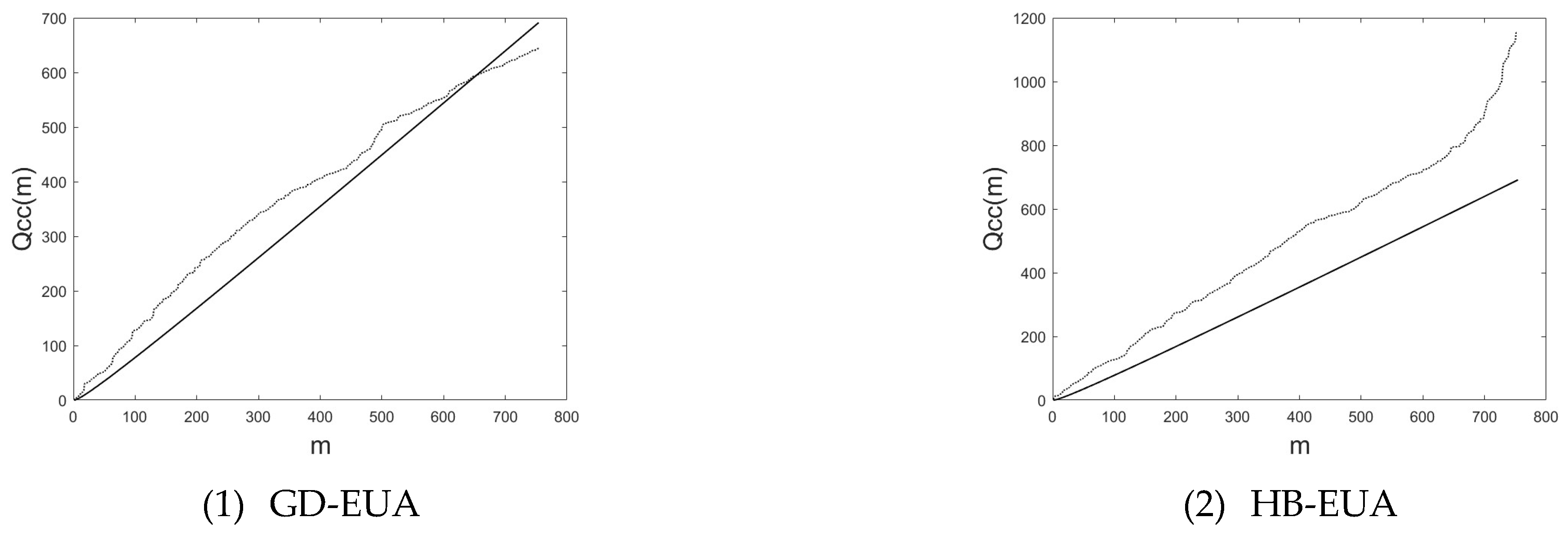
5.1. Cross-Correlation Test

The cross-correlations between GD-EUA and HB-EUA are first qualitatively analyzed in this study using the cross-correlation statistical test approach put forward by Podobnik et al. [17]. The GD-EUA and HB-EUA return series’ $Q_{cc}(m)$ against m and the chi-squared distribution’s critical values at a 5% significance level are shown in Figure 1. The graphic makes it clear that at the 5% significance level, the cross-correlation test statistics for the GD-EUA and HB-EUA return series are both above the critical value. Therefore, there is a long-term cross-correlation between the regression series.

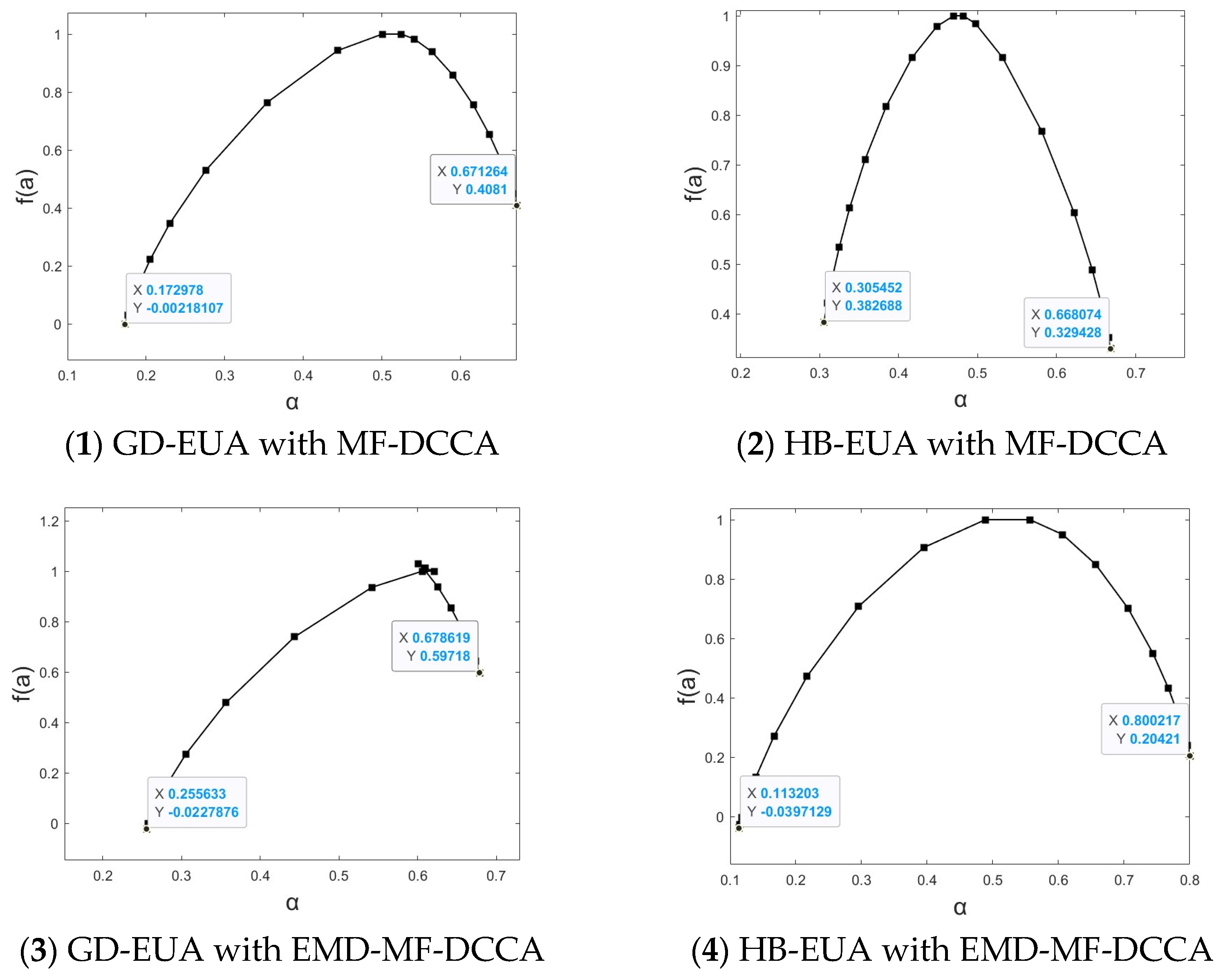
5.2. Cross-Correlation of Multiple Fractal Features

Based on an in-depth analysis of the statistical methods for testing cross-correlations, this study applied the MF-DCCA model and the EMD-MF-DCCA model, as described in Section 3. From Figure 2, our study reveals that, regardless of changes in the q values, the fluctuation curves rise significantly with increasing time scales. This shows that the fluctuation range of a time series increases with the extension of the time span. Additionally, for a range of q values, the log–log fluctuation curves show a broadly linear pattern, confirming a significant power-law cross-correlation between the returns from the Chinese carbon emission market and the EUA.

From

Table 2. Number of interrelationships.

q	MF-DCCA Method		EMD-MF-DCCA Method
	GD-EUA	HB-EUA	GD-EUA	HB-EUA
−10	0.612074238	0.601016823	0.638336613	0.720637866
−9	0.605497572	0.593566022	0.633860841	0.711795760
−8	0.597841228	0.58456948	0.628923317	0.701234052
−7	0.588923627	0.573513491	0.623601284	0.688469500
−6	0.578635205	0.559742604	0.618164641	0.672903769
−5	0.567089634	0.542690056	0.613266044	0.653938745
−4	0.554843097	0.52284656	0.610167946	0.631427177
−3	0.542985368	0.50347946	0.610641367	0.606519114
−2	0.532719171	0.48943375	0.615530332	0.581468008
−1	0.524290483	0.481618116	0.621611513	0.556460242
0	0.511469118	0.475065391	0.612970200	0.518683102
1	0.500321768	0.469733574	0.606105505	0.488778941
2	0.471852482	0.459096756	0.574131289	0.441791954
3	0.432547122	0.445100073	0.530703222	0.393065725
4	0.393425024	0.429932075	0.487237611	0.349072761
5	0.360752264	0.415461571	0.450914220	0.312618647
6	0.334839748	0.402587316	0.422529583	0.283651923
7	0.314296833	0.391501845	0.400508118	0.260919736
8	0.297792746	0.382067176	0.383178602	0.243007416
9	0.284331564	0.374042206	0.369276187	0.228726195
10	0.273196219	0.367183185	0.357911881	0.217173829
Δh	0.338878019	0.233833638	0.280424732	0.503464037

, when $q=-10,-9,\dots , 8, 9, 10$, the values of $H_{xy}(q)$ decrease as $q$ increases, indicating a high degree of multifractality between the returns of GD-EUA and HB-EUA. This suggests a nonlinear relationship between the Chinese and the EU carbon emission markets. The Hurst exponent $H_{xy}(2)$ for HB-EUA is 0.459096756 under the MF-DCCA model, and 0.441791954 under the EMD-MF-DCCA model, both of which are less than 0.5. This indicates that the two time series, the returns of the EUA and Hubei carbon emission allowance, are in an anti-persistent state, meaning that as Hubei carbon emission allowance prices rise, the EUA spot prices tend to decline. For GD-EUA, the $H_{xy}(2)$ is 0.471852482 under the MF-DCCA model, which is less than 0.5. But, using the EMD-MF-DCCA model, the $H_{xy}(2)$ for GD-EUA is 0.574131289. Therefore, there is an anti-persistent relationship between the long-term trends of the returns of the EUA and Guangdong carbon emission allowances, and a persistent relationship between their short-term fluctuations. Furthermore, when $q$ is small, the $H_{xy}(q)$ values of GD-EUA and HB-EUA are greater than 0.5. In contrast, when $q$ is large, the $H_{xy}(q)$ values of GD-EUA and HB-EUA are smaller than 0.5. Hence, for the Chinese and EU carbon emission markets, the persistence characteristics are displayed in the small fluctuation behaviors of the return series, while the larger fluctuations of the return series are anti-persistent.

Additionally, it can be observed that the Δh value for HB-EUA, calculated using the MF-DCCA method, is lower than that of GD-EUA. This indicates that the cross-correlation between carbon emission allowance returns in the EU and Guangdong markets exhibits a comparatively higher degree of fractality in the long term. In contrast, the Δh value for HB-EUA, calculated using the EMD-MF-DCCA method, is higher than that of GD-EUA. This suggests that, compared to the Guangdong carbon emission market, the cross-correlation between the Hubei and EU carbon emission markets displays stronger fractal characteristics in the short term. This primarily stems from differences in the types of traders and trading volumes between the carbon emission markets in Guangdong and Hubei. On one hand, based on the access conditions of different market participants in the carbon emission market, it can be seen that the similarity of traders in the Guangdong and EU carbon emission markets is relatively high, leading to similar trading behaviors and market performance. On the other hand, our analysis of trading volumes during the sample period reveals that the total trading volume of the Guangdong carbon emission market is 0.94 times that of the EU market, indicating a close similarity in trading volumes. However, the EU and Hubei carbon emission markets have a ratio of 0.32, indicating a significant difference in trading volumes. Therefore, compared to HB-EUA, the cross-correlation of GD-EUA exhibits a stronger fractal degree of fractality in the long term. This also reflects, to some extent, the stronger institutional coupling between the Guangdong and the EU carbon emission markets. Furthermore, the traders in the Hubei carbon emission market are mainly heavy industrial enterprises. As a result, the carbon emission allowance prices in the EU and Hubei markets are more likely to resonate when affected by sudden events (such as fluctuations in industrial activities and energy price shocks). This leads to a higher degree of fractality between the short-term fluctuations of the Hubei and EU carbon emission markets.

To present the data in Table 2 more intuitively, this study has created figures of $H_{xy}(q)$, ${\tau }_q$ and $q$. As demonstrated in Figure 3 and Figure 4, the $H_{xy}(q)$ and ${\tau }_q$ derived from the MF-DCCA and EMD-MF-DCCA methods both manifest non-linear characteristics, irrespective of the value of q. This further indicates the presence of multiple fractal characteristics between the Chinese and EU carbon emission markets. Specifically, under the MF-DCCA model, the nonlinearities of $H_{xy}(q)$ and ${\tau }_q$ of GD-EUA are more pronounced, while under the EMD-MF-DCCA model, the nonlinearities of $H_{xy}(q)$ and ${\tau }_q$ of HB-EUA are more pronounced. This also indicates that the cross-correlation of returns between the Guangdong and EU carbon emission markets exhibits stronger fractality in long-term trends, whereas the cross-correlation between the Hubei and EU carbon emission markets demonstrates stronger fractality in short-term fluctuations.

Figure 5 presents the multifractal spectra of the cross-correlations between GD-EUA and HB-EUA, revealing the complex dynamic mechanisms underlying the financial time series. A wider spectrum indicates stronger multifractal characteristics and higher market uncertainty, typically associated with stronger long-range cross-correlations. As observed in Figure 5, the fractal spectra of all sequences exhibit a downward-opening parabolic shape with significant spectrum widths, confirming the presence of pronounced multifractal characteristics between the GD-EUA and HB-EUA markets. Specifically, using the MF-DCCA and EMD-MF-DCCA methods, the spectrum widths of GD-EUA are 0.498286 and 0.422986, respectively, while those of HB-EUA is 0.362622 and 0.687014, respectively. This difference suggests that the long-term trends of the GD-EUA markets display more pronounced multifractal characteristics and uncertainty, whereas the HB-EUA markets predominantly demonstrate multifractal features and market complexity in the short-term fluctuations. This is consistent with the conclusions drawn earlier.

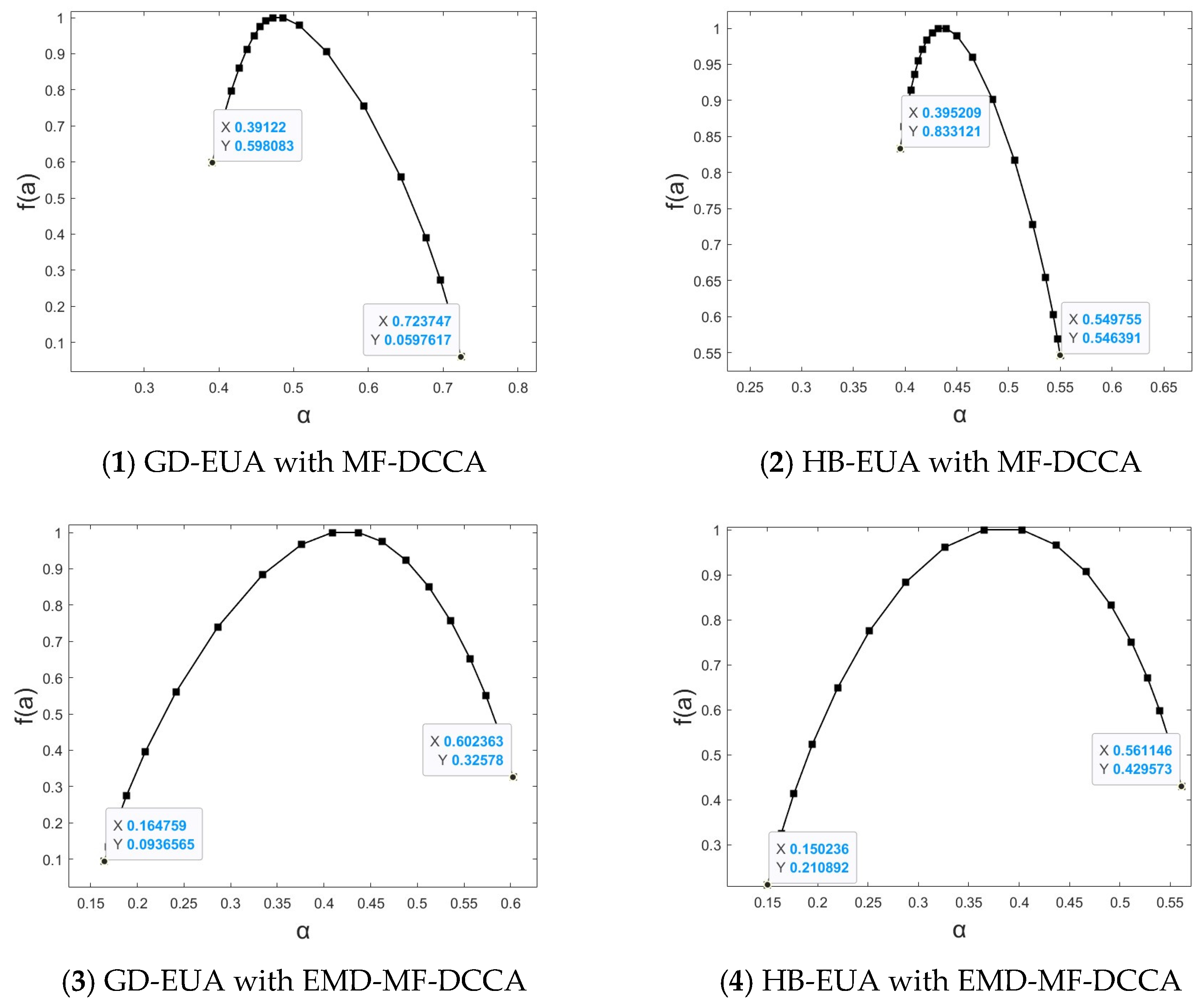
6. Multiple Fractal Source Analysis

Kantelhardt et al. [18] claim that the multifractality of financial time series is primarily caused by long-range correlations and the fat-tailed probability distribution of fluctuations. By comparing the multifractality intensity (Δh) and spectrum width (Δα) of the original series, the shuffled series, and the phase-randomized surrogate series, this study is able to determine the origins of multifractality. The long-range correlation of the original sequence can be destroyed while its distribution properties are retained through rearrangement. By randomly assigning a phase, the non-Gaussian nature of the original sequence can be weakened, and its long-range correlation can be preserved.

This approach allows us to identify which characteristics contribute most significantly to the observed multifractality.

Table 3. Multifractal intensity and spectral width.

	MF-DCCA				EMD-MF-DCCA
	GD-EUA		HB-EUA		GD-EUA		HB-EUA
	ΔH	Δα	ΔH	Δα	ΔH	Δα	ΔH	Δα
Original	0.338878019	0.362622	0.233833638	0.498286	0.280424732	0.422986	0.503464037	0.687014
Shuffled	0.224481172	0.366747	0.09249771	0.441052	0.258676593	0.39247	0.419479703	0.579661
Surrogate	0.198311338	0.332527	0.274066896	0.154546	0.27954758	0.437604	0.274956401	0.41091

and Figure 5, Figure 6 and Figure 7 present a detailed comparison of the Hurst exponent and multifractal spectra of the carbon emission allowance returns in the Chinese and the EU carbon emission markets. Then, this study finds that, compared to the original sequence, the Δh of the shuffled and surrogate sequences of GD-EUA is reduced, while the changes in Δα are very small. For HB-EUA, both Δh and Δα decrease noticeably, except that the Δh of the surrogate sequence derived from the MF-DCCA method increases slightly. These findings indicate that both the fat-tailed probability distributions and long-range correlations contribute to the multifractality of returns in the Chinese and EU carbon emission markets, with the effect being particularly pronounced for the cross-correlation between the Hubei and EU carbon emission markets.

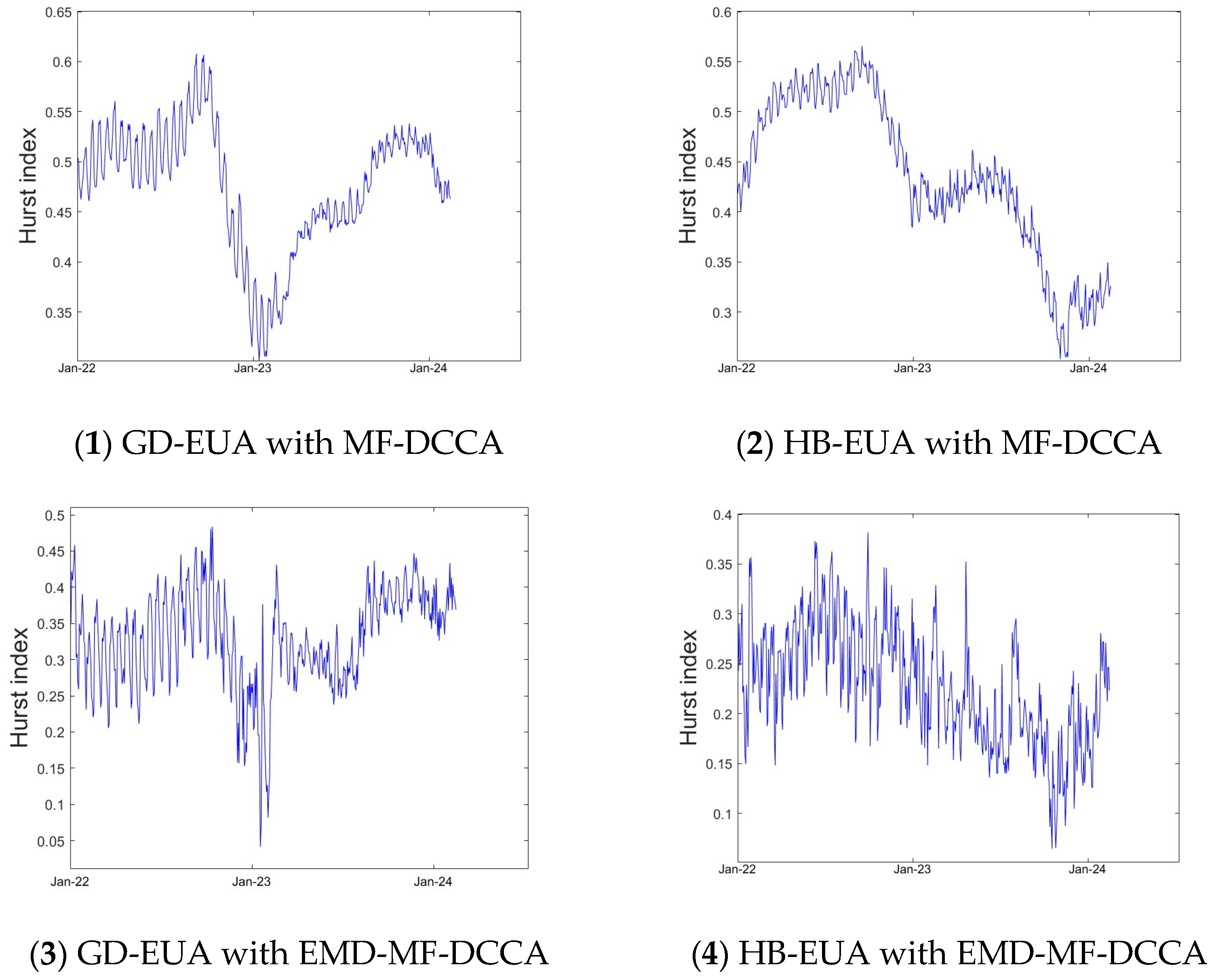
7. Sliding Window Analysis

The carbon emission allowance prices in China and the EU have a nonlinear relationship, according to the previous findings of this study. Therefore, a sliding window approach is employed in order to further investigate their interrelationship. This study selected a window length of 250 days with a q value of two to compute the cross-correlation index. The daily cross-correlation indices, calculated using the MF-DCCA and EMD-MF-DCCA models, are plotted in Figure 8, where the dynamic variations in the cross-correlations between HB-EUA and GD-EUA are depicted. According to the analysis, the Hurst exponent is typically less than 0.5 during the sample period, suggesting a primarily negative link between the carbon emission markets in China and Europe.

The Hurst exponent for carbon emission markets in China and the EU showed a steady decline from June 2022 to January 2023, indicating reduced long-term memory, lower predictability, and greater market efficiency. This trend is linked to national policies, particularly the Ministry of Ecology and Environment’s June 2022 plan for pollution reduction and carbon control, which strengthened the Chinese carbon market management, fostered market growth, and improved efficiency. However, between January and May 2023, the volatility of GD-EUA increased significantly, while the volatility of HB-EUA remained relatively stable. This discrepancy suggests that while national policies have improved overall market efficiency, regional carbon emission markets may react differently. Specifically, the carbon emission market exhibited higher efficiency under the policy influence, whereas the trading volume in the Guangdong carbon emission market decreased compared to previous periods.

From May to October 2023, there were notable differences between the Hurst indices of GD-EUA and HB-EUA. Specifically, the Hurst index for GD-EUA exhibited a relatively stable trend, whereas the Hurst index for HB-EUA showed a downward trend. This decline indicates an increase in price volatility within the Hubei’s carbon emission market, reflecting a strengthening of anti-persistence characteristics. The study attribute this phenomenon primarily to individual traders. In May 2023, the Hubei carbon emission rights market implemented a significant policy adjustment, reducing transaction fees for individual traders by 50%. The market participants’ reactions and expectations regarding this policy also influenced the market volatility. This policy change altered participants’ expectations for the Hubei carbon emission market, leading them to engage more actively in trading in the short term. The resulting increase in liquidity is typically associated with amplified price volatility, which directly contributed to the decrease in the Hurst index.

The Hubei carbon emission market is more efficient than the Guangdong carbon emission market, according to the aforementioned findings. Therefore, in developing the Chinese carbon emission market, policy directions and implementations should align more closely with those of the Hubei carbon emission market to promote further advancement of the national carbon emission market.

8. Conclusions and Recommendations

8.1. Conclusions

In this study, the relationship between the EU and the Chinese carbon emission markets is examined using the MF-DCCA and EMD-MF-DCCA methods. The study yields several key findings.

Firstly, using the MF-DCCA and EMD-MF-DCCA methods, it can be found that the Chinese carbon emission market and the EU carbon emission market exhibit a significant power-law interrelationship, which demonstrates significant multifractal characteristics. Specifically, the cross-correlation between the long-term trends of returns of the Guangdong and EU carbon emission markets exhibits stronger fractality, whereas the cross-correlation between the short-term fluctuations of the Hubei and EU carbon emission markets demonstrates stronger fractality.

Secondly, when investigating the underlying causes of multifractal characteristics, the findings of this study indicate that these features primarily stem from the fat-tailed distribution and long-memory property of the data. Compared with the Guangdong carbon emission market, these two factors have more of an influence on the multifractal degree between the Hubei and EU carbon markets. This conclusion underscores the importance of considering the data distribution characteristics in the analysis of financial time series while also revealing the deeper dynamic mechanisms behind market behavior.

Lastly, the Hurst index between the EU and the Chinese carbon emission markets is typically less than 0.5, according to the rolling window analysis. This result indicates a significant inverse and persistent relationship between these markets. Notably, although the efficiency of the Chinese carbon emission market is currently relatively low, there is evidence of gradual improvement. This suggests that the Chinese carbon emission market is advancing toward greater maturity and efficiency, with ongoing enhancements in market mechanisms and proactive policy measures. Additionally, the Hubei carbon emission market is found to be more efficient than the Guangdong carbon emission market.

8.2. Recommendations

It is clear from the aforementioned conclusions that, in comparison to the carbon emission market in the European Union, the Chinese carbon emission market needs further growth. This study offers the following recommendations for the Chinese carbon emission market:

First, the Ministry of Ecology and Environment’s departmental regulations now serve as the primary legal foundation for the Chinese carbon emission market. These laws have little legal force and make it challenging to ensure that the carbon emission market operates in a stable and effective manner over the long run. Therefore, it is essential to establish a comprehensive legal system to regulate the behavior of market participants, ensure fairness and transparency in transactions, and foster the healthy and stable development of the carbon emission market. Additionally, China must strengthen the regulatory capacity of its institutions, implement effective market supervision, and manage risks, with a particular focus on the short-term fluctuation risks in the Hubei carbon emission market. These measures are crucial for providing a stable operational environment for the carbon emission markets. Not only will they improve market efficiency, but they will also strengthen investor confidence, thereby attracting more capital into the market.

Second, the Hubei carbon emission market is shown to be more efficient than the Guangdong carbon emission market. This is primarily because it places more focus on the growth of individual traders, a feature that is also present in the EU carbon emission market. Thus, it is recommended that the Chinese carbon emission market increase opportunities for individual traders. To further invigorate the market and attract more individual traders, it is recommended that the Chinese carbon emission market further reduce the handling fees of carbon trading and implement tax incentives and other incentives. These measures would enhance individual traders’ activity, improve market liquidity, lower transaction costs, and boost market efficiency, thereby supporting the healthy development of the Chinese carbon emission market and achieving the carbon emission reduction objectives.

References

1. Sun, L.; Xiang, M.; Shen, Q. A comparative study on the volatility of EU and China’s carbon emission permits trading markets. Phys. A Stat. Mech. Appl. 2020, 560, 125037. [Google Scholar] [CrossRef]
2. Zhu, D.; Zhang, C.; Pan, D.; Hu, S. Multifractal cross-correlation analysis between carbon spot and futures markets considering asymmetric conduction effect. Fractals 2021, 29, 2150176. [Google Scholar] [CrossRef]
3. Meng, J.; Hu, S.; Mo, B. Dynamic tail dependence on China’s carbon market and EU carbon market. Data Sci. Financ. Econ. 2021, 1, 393–407. [Google Scholar] [CrossRef]
4. Wu, X.; Zhu, Z. Time-varying risk aversion and dynamic dependence between crude oil futures and European Union allowance futures markets. Front. Environ. Sci. 2023, 11, 1152761. [Google Scholar] [CrossRef]
5. Benz, E.; Trück, S. Modeling the price dynamics of CO2 emission allowances. Energy Econ. 2009, 31, 4–15. [Google Scholar] [CrossRef]
6. Yu, J.; Mallory, M.L. Carbon price interaction between allocated permits and generated offsets. Oper. Res. 2020, 20, 671–700. [Google Scholar] [CrossRef]
7. Zhu, B.; Han, D.; Wang, P.; Wu, Z.; Zhang, T.; Wei, Y.M. Forecasting carbon price using empirical mode decomposition and evolutionary least squares support vector regression. Appl. Energy 2019, 191, 521–530. [Google Scholar] [CrossRef]
8. Yu, L.; Li, C.; Wang, J.; Sun, H. A hybrid model for predicting the carbon price in Beijing: A pilot low-carbon city in China. Front. Phys. 2024, 12, 1427794. [Google Scholar] [CrossRef]
9. Qi, S.; Cheng, S.; Tan, X.; Feng, S.; Zhou, Q. Predicting China’s carbon price based on a multi-scale integrated model. Appl. Energy 2022, 324, 119784. [Google Scholar] [CrossRef]
10. Sun, W.; Huang, C. A carbon price prediction model based on secondary decomposition algorithm and optimized back propagation neural network. J. Clean. Prod. 2020, 243, 118671. [Google Scholar] [CrossRef]
11. Zhou, W. Multifractal detrended cross-correlation analysis for two nonstationary signals. Phys. Rev. E 2008, 77, 066211. [Google Scholar] [CrossRef] [PubMed]
12. Zou, S.; Zhang, T. Multifractal Detrended Cross-Correlation Analysis of Electricity and Carbon Markets in China. Math. Probl. Eng. 2019, 1, 13. [Google Scholar] [CrossRef]
13. An, Y.; Jiang, K.; Song, J. Does a Cross-Correlation of Economic Policy Uncertainty with China’s Carbon Market Really Exist? A Perspective on Fractal Market Hypothesis. Sustainability 2023, 15, 10818. [Google Scholar] [CrossRef]
14. Fan, X.; Lv, X.; Yin, J.; Tian, L.; Liang, J. Multifractality and market efficiency of carbon emission trading market: Analysis using the multifractal detrended fluctuation technique. Appl. Energy 2019, 251, 113333. [Google Scholar] [CrossRef]
15. Podobnik, B.; Stanley, H.E. Detrended cross-correlation analysis: A new method for analyzing two nonstationary time series. Phys. Rev. Lett. 2008, 100, 084102. [Google Scholar] [CrossRef] [PubMed]
16. Podobnik, B.; Grosse, I.; Horvatić, D.; Ilic, S.; Ivanov, P.C.; Stanley, H.E. Quantifying cross-correlations using local and global detrending approaches. Eur. Phys. J. B 2009, 71, 243–250. [Google Scholar] [CrossRef]
17. Shadkhoo, S.; Jafari, G.R. Multifractal detrended cross-correlation analysis of temporal and spatial seismic data. Eur. Phys. J. B 2009, 72, 679–683. [Google Scholar] [CrossRef]
18. Kantelhardt, J.; Zschiegner, S.; Bunde, E.K.; Havlin, S.; Bunde, A.; Stanley, H.E. Multifractal Detrended Fluctuation Analysis of Nonstationary Time Series. Phys. A Stat. Mech. Appl. 2002, 316, 87–114. [Google Scholar] [CrossRef]
Figure 1. Results of the cross-correlation statistical test. Note: The curve represents the value of the correlation measurement Q c c ( m ) , and the straight line is the critical value of the correlation measurement.
Fractalfract 09 00326 g001
Figure 2. Multifractal analysis of the cross-correlation of carbon emission markets in China and the EU. Note: The values of q corresponding to the fluctuation curve from bottom to top are q = −5, −4, …, 4, 5, respectively.
Fractalfract 09 00326 g002
Figure 3. Mutual correlation indices of HB-EUA and GD-EUA. Note: The orange line represents the value of Guangdong and EUA, and the blue line is the value of Hubei and EUA.
Fractalfract 09 00326 g003
Figure 4. Cross-correlations of HB-EUA and GD-EUA in τ(q) vs. q. Note: The orange line represents the value for Guangdong and EUA, while the blue line shows the value for Hubei and EUA.
Fractalfract 09 00326 g004
Figure 5. Multiple fractal spectra of the HB-EUA and GD-EUA cross-correlations.
Fractalfract 09 00326 g005
Figure 6. Multiple fractal spectra of HB-EUA and GD-EUA cross-correlations for shuffled sequences.
Fractalfract 09 00326 g006
Figure 7. Multiple fractal spectra of HB-EUA and GD-EUA cross-correlations for surrogate sequences.
Fractalfract 09 00326 g007
Figure 8. Dynamics of the Hurst index when q = 2.
Fractalfract 09 00326 g008