Article

A New L2 Type Difference Scheme for the Time-Fractional Diffusion Equation

Department of Mathematics, Shantou University, Shantou 515063, China
*
Author to whom correspondence should be addressed.
Fractal Fract. 2025, 9(5), 325; https://doi.org/10.3390/fractalfract9050325
Submission received: 18 March 2025 / Revised: 4 May 2025 / Accepted: 10 May 2025 / Published: 20 May 2025

Abstract

In this paper, a new L2 (NL2) scheme is proposed to approximate the Caputo temporal fractional derivative, leading to a time-stepping scheme for the time-fractional diffusion equation (TFDE). Subsequently, the space derivative of the resulting system is discretized using a specific finite difference method, yielding a fully discrete system. We then establish the H 1 -norm stability and convergence of the time-stepping scheme on uniform meshes for the TFDE. In particular, we prove that the proposed scheme has ( 3 α ) th-order accuracy, where α ( 0 < α < 1 ) is the order of the time-fractional derivative. Finally, numerical experiments for several test problems are carried out to validate the obtained theoretical results.

1. Introduction

In this paper, we consider numerical methods for the time-fractional diffusion equation with variable coefficients:
0 t α u ( x , t ) = x p ( x ) u x q ( x ) u ( x , t ) + f ( x , t ) , ( x , t ) ( 0 , l ) × ( 0 , T ] , u ( 0 , t ) = 0 , u ( l , t ) = 0 , 0 t T , u ( x , 0 ) = u 0 ( x ) , x [ 0 , l ] ,
where p ( x ) C 1 > 0 and q ( x ) 0 , f ( x , t ) is the source term, and 0 t α u ( x , t ) is the Caputo derivative of order α ( 0 < α < 1 ) with respect to t, i.e.,
0 t α u ( x , t ) = 1 Γ ( 1 α ) 0 t u ( x , η ) η ( t η ) α d η .
Here, Γ ( α ) = 0 t α 1 e t d t is the Γ function.
Fractional partial differential equations (FPDEs) have extensive applications in diverse fields, as illustrated in references [1,2,3,4,5,6,7,8]. Specifically, the time-fractional diffusion equation (TFDE) overcomes the limitations of traditional integer-order calculus. It offers a general mathematical framework for depicting complex systems exhibiting non-locality, long-range correlations, and memory effects. The time-fractional diffusion equation poses a significant challenge since it is an integro-differential equation, whose analytical solution is often difficult to derive. Consequently, numerical methods are necessary for its solution. Several approaches have been developed to solve the TFDE. For example, Ahmad et al. [8] introduced Monte Carlo-based physics-informed neural networks with the cuckoo search (PINN-CS) algorithm for addressing fractional partial differential equations. Sun and Wu [9] introduced and analyzed a finite difference scheme for the fractional diffusion wave equation. Lin and Xu [10] proposed a numerical scheme using a finite difference scheme in time and Legendre spectral methods in space. Zhang and Sun [11] presented an alternating direction implicit scheme. Sun et al. [12] devised finite difference schemes for a variable-order time fractional diffusion equation. Yan, Pal, and Ford [13] developed a ( 3 α ) th-order method by directly discretizing the fractional differential operator. Li and Liao [14] analyzed the well-known differential equations by applying the corresponding inverse operators.
Recently, research on numerical methods for Caputo fractional derivatives has increased significantly; see, e.g., [15,16,17,18,19,20,21,22,23]. Gao et al. developed a novel difference analog of the Caputo fractional derivative, known as the L1-2 formula [24]. Alikhanov used piecewise quadratic polynomial interpolation to derive the L2-1 σ formula for approximating the Caputo fractional derivative at specific points [25]. The schemes proposed in [17,20,23,24,25] have been proven to have 3 α order accuracy for α th-order Caputo fractional derivatives. Notably, Quan and Wu [23] established H 1 -norm stability and convergence for an L2 scheme on general nonuniform meshes when applied to the subdiffusion equation. We noticed that the discrete form of these schemes at the first step t 1 = τ or the last step differs from the unified form for the rest of the steps. As an example, in [20], the approximation of the first time step is obtained by using the L1-formula on the time layer [ 0 , τ ] with step size τ 1 = O ( τ 3 α 2 α ) . To address this issue and preserve the order of convergence, we propose a scheme using piecewise quadratic polynomial interpolation, which computes approximate values in pairs. We call it the new L2 (NL2) discretization. We showed that the NL2 scheme’s discretization matrix is a block lower triangular Toeplitz matrix with two-by-two blocks and proved its H 1 -norm stability and convergence. Numerical experiments show that the NL2 scheme has better accuracy than the L2 schemes proposed in [17,20].
The rest of this paper is organized as follows: In Section 2, we propose a novel piecewise quadratic polynomial interpolation method, referred to as the new L2 scheme (NL2 for short), to approximate the Caputo fractional derivative. Subsequently, we derive the key properties of the NL2 scheme, including its consistency and the features of the discretization matrix. Section 3 presents a difference scheme based on the NL2 scheme, deriving its H 1 -norm stability. In Section 4, we conduct numerical experiments to verify the theoretical findings of the proposed scheme. Finally, Section 5 offers concluding remarks.

2. A Novel L2 Scheme for the Caputo Derivative

Let α ( 0 , 1 ) and v ( t ) be a function in C 3 ( 0 , T ] . Consider approximating the Caputo fractional derivative of order α defined by (2).

2.1. A New L2 Scheme

Let M be a positive integer and τ = T / ( 2 M ) . Define a uniform grid
t k = k τ , k = 0 , 1 , , 2 M .
Denote v ( t i ) by v i and the quadratic interpolation polynomial of v ( t ) at the points ( t 2 i 2 , v 2 i 2 ) , ( t 2 i 1 , v 2 i 1 ) and ( t 2 i , v 2 i ) by Π 2 , i v ( t ) . We have
Π 2 , i v ( t ) = ( t t 2 i 1 ) ( t t 2 i ) 2 τ 2 v 2 i 2 ( t t 2 i 2 ) ( t t 2 i ) τ 2 v 2 i 1 + ( t t 2 i 2 ) ( t t 2 i 1 ) 2 τ 2 v 2 i .
Assume v ( · ) C 3 ( 0 , T ] , then we have
v ( t ) Π 2 , i v ( t ) = v ( ξ i ) 6 ( t t 2 i 2 ) ( t t 2 i 1 ) ( t t 2 i ) ,
where t , ξ i [ t 2 i 2 , t 2 i ] , and ξ i depends on t , 1 i M . We arrive at
( Π 2 , i v ( t ) ) = δ v 2 i 1 2 + δ 2 v 2 i 1 ( t t 2 i 1 2 ) , t [ t 2 i 2 , t 2 i ] ,
where
δ v 2 i 1 2 = v 2 i v 2 i 1 τ , δ 2 v 2 i 1 = δ v 2 i 1 2 δ v 2 i 3 2 τ = v 2 i 2 v 2 i 1 + v 2 i 2 τ 2 .
Now, we introduce the discretization of the Caputo derivative. It is easy to obtain
α v ( t ) t α t = t 2 k 1 = 1 Γ ( 1 α ) 0 t 2 k 1 v ( η ) η ( t 2 k 1 η ) α d η = 1 Γ ( 1 α ) i = 1 k 1 t 2 i 2 t 2 i v ( η ) η ( t 2 k 1 η ) α d η + t 2 k 2 t 2 k 1 v ( η ) η ( t 2 k 1 η ) α d η
and
α v ( t ) t α t = t 2 k = 1 Γ ( 1 α ) i = 1 k t 2 i 2 t 2 i v ( η ) η ( t 2 k η ) α d η
for k = 1 , 2 , , M .
From the above expression, we approximate v ( t ) by making use of Π 2 , i v ( t ) on the interval [ t 2 i 2 , t 2 i ] ( 1 i M ) . Firstly, we have
t 2 i 1 t 2 i ( t j η ) α d η = τ 1 α 1 α a j 2 i + 1 , j 2 i ,
where
a k = ( 1 α ) 0 1 ( k s ) α d s = k 1 α ( k 1 ) 1 α , k 1 .
Let
g ( r , s ) = ( r s ) α ( r + s ) α , r 1 2 , 0 s 1 2 ,
and let
b k = ( 1 α ) 0 1 2 g k 1 2 , s s d s = 1 2 α [ k 2 α ( k 1 ) 2 α ] 1 2 [ k 1 α + ( k 1 ) 1 α ] , k 1 .
Then, we have
t 2 i 1 t 2 i ( t j η ) α ( η t 2 i 1 2 ) d η = τ 2 α 1 α b j 2 i + 1 , j 2 i .
Based on the above discussion, we obtain
t 2 i 2 t 2 i ( t j η ) α ( Π 2 , i v ( η ) ) d η = t 2 i 2 t 2 i ( t j η ) α δ v 2 i 1 2 + δ 2 v 2 i 1 ( η t 2 i 1 2 ) d η = t 2 i 2 t 2 i 1 ( t j η ) α d η + t 2 i 1 t 2 i ( t j η ) α d η δ v 2 i 1 2 + t 2 i 2 t 2 i 1 ( t j η ) α ( η t 2 i 1 2 ) d η + t 2 i 1 t 2 i ( t j η ) α ( η t 2 i 1 2 ) d η δ 2 v 2 i 1 = τ 1 α 1 α [ ( a j 2 i + 1 + a j 2 i + 2 ) δ v 2 i 1 2 + τ ( b j 2 i + 1 + b j 2 i + 2 a j 2 i + 2 ) δ 2 v 2 i 1 ] = τ 1 α 1 α [ ( a j 2 i + 2 b j 2 i + 1 b j 2 i + 2 ) δ v 2 i 3 2 + ( a j 2 i + 1 + b j 2 i + 1 + b j 2 i + 2 ) δ v 2 i 1 2 ]
and
t 2 k 2 t 2 k 1 v ( η ) η ( t 2 k 1 η ) 1 α d η = τ 1 α 1 α [ ( a 1 b 1 ) δ v 2 k 3 2 + b 1 δ v 2 k 1 2 ] .
Finally, from (3), we obtain
α v ( t ) t α t = t 2 k 1 ( L α v ) ( t 2 k 1 ) : = τ 1 α Γ ( 2 α ) i = 1 k 1 ( a 2 k 2 i + 1 b 2 k 2 i b 2 k 2 i + 1 ) δ v 2 i 3 2 + ( a 2 k 2 i + b 2 k 2 i + b 2 k 2 i + 1 ) δ v 2 i 1 2 + τ 1 α Γ ( 2 α ) ( a 1 b 1 ) δ v 2 k 3 2 + b 1 δ v 2 k 1 2 = τ 1 α Γ ( 2 α ) i = 1 k 1 c 2 k 2 i + 1 δ v 2 i 3 2 + i = 1 k 1 d 2 k 2 i δ v 2 i 1 2 + ( a 1 b 1 ) δ v 2 k 3 2 + b 1 δ v 2 k 1 2 ,
where
c 1 = a 1 b 1 , c k = a k b k b k 1 , k 2
and
d 1 = b 1 , d k = a k 1 + b k 1 + b k , k 2 .
Similarly, from (4), we obtain
α v ( t ) t α t = t 2 k ( L α v ) ( t 2 k ) : = τ 1 α Γ ( 2 α ) i = 1 k ( c 2 k 2 i + 2 δ v 2 i 3 2 + d 2 k 2 i + 1 δ v 2 i 1 2 )
for k = 1 , 2 , , M .
Let
L α v = ( L α v ) ( t 1 ) , ( L α v ) ( t 2 ) , , ( L α v ) ( t 2 M ) T , v t = ( δ v 1 2 , δ v 3 2 , δ v 5 2 , , δ v 2 M 1 2 ) T ,
and B be a matrix defined by
B = c 1 d 1 0 0 0 0 0 0 c 2 d 2 0 0 0 0 0 0 c 3 d 3 c 1 d 1 0 0 0 0 c 4 d 4 c 2 d 2 0 0 0 0 c 5 d 5 c 3 d 3 c 1 d 1 0 0 c 6 d 6 c 4 d 4 c 2 d 2 0 0 c 2 M 1 d 2 M 1 c 2 M 3 d 2 M 3 c 2 M 5 d 2 M 5 c 1 d 1 c 2 M d 2 M c 2 M 2 d 2 M 2 c 2 M 4 d 2 M 4 c 2 d 2 .
Then, we obtain the matrix form of the NL2 scheme for the Caputo fractional derivative
L α v = μ B v t ,
where μ = τ 1 α Γ ( 2 α ) . It can be seen that B is a block lower triangular Toeplitz matrix with 2 × 2 blocks.

2.2. Basic Properties of Relevant Coefficients

In this subsection, we establish certain properties of the coefficients in the NL2 scheme, which are useful in analyzing the convergence and stability of the NL2 scheme.
We need the following results. Assuming 0 < x < 1 and α ( 0 , 1 ) , we have
( 1 x ) 2 α = 1 ( 2 α ) x + k = 2 g k ( 2 α ) x k ,
where g 2 ( 2 α ) = ( 2 α ) ( 1 α ) 2 and 0 < g k ( 2 α ) = α + k 3 k g k 1 ( 2 α ) < g k 1 ( 2 α ) for k 3 . Moreover,
( 1 x ) 1 α = 1 k = 1 g k ( 1 α ) x k ,
where g 1 ( 1 α ) = 1 α and 0 < g k ( 1 α ) = α + k 2 k g k 1 ( 1 α ) < g k 1 ( 1 α ) for k 2 . We obtain
g k ( 2 α ) = 2 α α + k 2 g k ( 1 α )
for k 2 .
Lemma 1. 
(Properties of a k , b k , c k and d k ). The following properties of the coefficients of the NL2 scheme in (7) and (8) hold:
(1) 1 = a 1 > a 2 > a 3 > > a k > 0 ;
(2) b 1 > b 2 > b 3 > > b k > 0 ;
(3) d 2 > d 3 > d 4 > > d k > 0 ;
(4) c 3 > c 4 > c 5 > > c k > 0 ;
(5) c 1 = 4 3 α 2 ( 2 α ) > 0 , c 2 = ( 2 3 α ) 2 1 α 2 ( 2 α ) ( 1 2 , 1 ) , d 1 = α 2 ( 2 α ) > 0 .
Proof. 
(1) By (5), the conclusion is easy to obtain from a k = ( 1 α ) 0 1 ( k 1 + s ) α d s for k 1 .
(2) From g ( r , s ) = ( r s ) α ( r + s ) α , we see that g ( r , s ) > 0 for s ( 0 , 1 2 ) , and it follows from (6) that b k > 0 for k 1 . Furthermore, we have
g r = α [ ( r s ) ( α + 1 ) ( r + s ) ( α + 1 ) ] < 0 , r 1 2 , 0 < s 1 2 .
Therefore, g ( r , s ) is a strictly monotonically decreasing function with respect to r. In particular, g k + 1 2 , s < g k 1 2 , s for k 1 , s ( 0 , 1 / 2 ] . By (6) again, we obtain b k + 1 < b k for k = 1 , 2 , .
(3) From (1) and (2), we obtain
d k = a k 1 + b k 1 + b k > 0
and
d k + 1 d k = a k a k 1 + b k + 1 b k 1 < 0
for k > 1 .
(4) For { c k } , k 3 , by using (9) and (10), we have
c k = 1 2 α [ k 2 α ( k 2 ) 2 α ] + 3 2 k 1 α + 1 2 ( k 2 ) 1 α = k 2 α 2 α + k 2 α 2 α ( 1 2 k ) 2 α + 3 2 k 1 α + k 1 α 2 ( 1 2 k ) 1 α > k 2 α 2 α + k 2 α 2 α 1 2 ( 2 α ) k + 2 ( 2 α ) ( 1 α ) k 2 + 3 k 1 α 2 + k 1 α 2 1 2 ( 1 α ) k ( 1 α ) α 2 j = 2 ( 2 k ) j = ( 1 α ) 1 α k 2 k α > 0 .
Now, we consider the monotonicity of { c k } , k 3 . We have
c k c k 1 = k 2 α 2 α + k 2 α 2 α ( 1 1 k ) 2 α + k 2 α 2 α ( 1 2 k ) 2 α k 2 α 2 α ( 1 3 k ) 2 α + 3 2 k 1 α 3 k 1 α 2 ( 1 1 k ) 1 α + k 1 α 2 ( 1 2 k ) 1 α k 1 α 2 ( 1 3 k ) 1 α
for k 4 . By using (9)–(11), we have
c k c k 1 = 2 g 2 ( 1 α ) k 1 + α 5 g 3 ( 1 α ) k 2 + α 8 g 4 ( 1 α ) k 3 + α 11 g 5 ( 1 α ) 3 k 4 + α + j = 6 g j ( 1 α ) k 1 α j + 1 ( 1 k ) j + 2 ( 2 k ) j 3 ( 3 k ) j + j = 6 g j ( 1 α ) k 1 α 2 3 ( 1 k ) j ( 2 k ) j + ( 3 k ) j < 2 g 2 ( 1 α ) k 1 + α + j = 6 g j ( 1 α ) k 1 α 2 3 ( 1 k ) j + ( 3 k ) j < α ( 1 α ) k 1 + α + g 6 ( 1 α ) k 1 α 2 j = 6 3 ( 1 k ) j + ( 3 k ) j < α ( 1 α ) k 1 + α + ( 1 α ) α k 1 α 12 3 k 5 ( k 1 ) + 3 6 k 5 ( k 3 ) = 1 4 k 3 ( k 1 ) + 3 5 4 k 3 ( k 3 ) 1 α ( 1 α ) k 1 + α < 123 2 k 3 1 α ( 1 α ) k 1 + α < 0 .
(5) Obviously, c 1 > 0 , d 1 > 0 for 0 < α < 1 , and
c 2 = ( 2 3 α ) 2 1 α 2 ( 2 α ) = 2 3 α 2 α ( 2 α ) .
Let g ( α ) = 2 3 α 2 α ( 2 α ) , 0 α 1 , then
g ( α ) = [ 4 + ( 3 α 2 8 α + 4 ) ln 2 ] 2 α ( 2 α ) 2 < 0 , 0 α 1 .
Hence, the function g ( α ) is a monotonically decreasing function with respect to α , and g ( α ) [ 1 2 , 1 ] . Consequently c 2 ( 1 2 , 1 ) for α ( 0 , 1 ) . □

2.3. Consistency of the NL2 Scheme

In this subsection, we prove the consistency of the NL2 scheme for the Caputo derivative, and it can achieve ( 3 α ) th-order accuracy.
Theorem 1. 
Let α ( 0 , 1 ) , k = 2 M , and v ( t ) C 3 [ 0 , T ] , then
| 0 t α v ( t k ) ( L α v ) ( t k ) | max 0 t T | v ( t ) | 6 Γ ( 2 α ) 1 α + 2 1 α α τ 3 α .
Proof. 
For k = 2 M , we have
0 t α v ( t 2 M ) ( L α v ) ( t 2 M ) = 1 Γ ( 1 α ) i = 1 M t 2 i 2 t 2 i ( t 2 M η ) α [ v ( η ) Π 2 , i v ( η ) ] d η = 1 Γ ( 1 α ) i = 1 M t 2 i 2 t 2 i ( t 2 M η ) α d [ v ( η ) Π 2 , i v ( η ) ] = α 6 Γ ( 1 α ) i = 1 M t 2 i 2 t 2 i v ( ξ i ) ( η t 2 i 2 ) ( η t 2 i 1 ) ( η t 2 i ) ( t 2 M η ) α 1 d η ,
where ξ i [ t 2 i 2 , t 2 i ] . It follows that
| 0 t α v ( t 2 M ) ( L α v ) ( t 2 M ) | α max 0 t T | v ( t ) | 6 Γ ( 1 α ) i = 1 M t 2 i 2 t 2 i | ( η t 2 i 2 ) ( η t 2 i 1 ) ( η t 2 i ) ( t 2 M η ) α 1 | d η .
It is easy to obtain
| ( η t 2 i 2 ) ( η t 2 i 1 ) ( η t 2 i ) | 2 3 τ 3 9 , η [ t 2 i 2 , t 2 i ] .
Therefore,
i = 1 M 1 t 2 i 2 t 2 i | ( η t 2 i 2 ) ( η t 2 i 1 ) ( η t 2 i ) ( t 2 M η ) α 1 | d η i = 1 M 1 2 3 τ 3 9 t 2 i 2 t 2 i ( t 2 M η ) α 1 d η = 2 3 τ 3 9 α ( 2 τ ) α t 2 M α τ 3 α α .
As for the last term of (12), we have
t 2 M 2 t 2 M | ( η t 2 M 2 ) ( η t 2 M 1 ) ( η t 2 M ) ( t 2 M η ) α 1 | d η = t 2 M 2 t 2 M | 2 τ ( t 2 M η ) τ ( t 2 M η ) ( t 2 M η ) α | d η = 0 2 τ ( 2 τ s ) | τ s | s α d s 2 2 α τ 3 α 1 α .
Combining (12), (13), and (14), we have
0 t α v ( t 2 M ) ( L α v ) ( t 2 M ) max 0 t T | v ( t ) | 6 Γ ( 2 α ) 1 α + 2 2 α α τ 3 α .

3. A Difference Scheme for the TFDE Based on the NL2 Scheme

In this section, we introduce the NL2 scheme for the time-fractional diffusion equation with variable coefficients Equation (1).
Let h = ( x R x L ) / N and τ = T / ( 2 M ) be the size of spatial grid and the length of time step, respectively, where N and M are positive integers. Define the following spatial and temporal grids:
x n = n h , n = 0 , 1 , , N ; t k = k τ , k = 0 , 1 , , 2 M .
In the following, we use the notations
u n k = u ( x n , t k ) , p n = p ( x n ) , q n = q ( x n ) , f n k = f ( x n , t k ) .
Applying the new L2 scheme to discretize the temporal derivative, the TFDE (1) is written as
( L α u ) ( x , t k ) = x ( p u x ) k q u k + f k , x ( 0 , l ) , u 0 k = 0 , u N k = 0 , 0 t k T , u ( x , t 0 ) = u 0 , x ( 0 , l ) ,
where p = p ( x ) , q = q ( x ) , u k = u ( x , t k ) and f k = f ( x , t k ) for k = 1 , 2 , , 2 M .
Lemma 2 
([25]). Let p ( x ) C 3 [ 0 , l ] and u ( x ) C 4 [ 0 , l ] , then the following equality holds true:
x p ( x ) u ( x ) x | x = x i = p ( x i + 1 / 2 ) u ( x i + 1 ) ( p ( x i + 1 / 2 ) + p ( x i 1 / 2 ) ) u ( x i ) + p ( x i 1 / 2 ) u ( x i 1 ) h 2 + O ( h 2 ) .
We use the above finite difference method in the spatial direction; then, we construct an NL2 scheme for Equation (15) with an accuracy of order O ( h 2 + τ 3 α ) .

3.1. The Positive Definiteness of B + B T

In this subsection, we study the positive definiteness of the symmetric part of matrix B, equivalently, the positive definiteness of B + B T .
Lemma 3 
([21]). Given an arbitrary symmetric matrix S R n × n with positive elements. If S satisfies the following properties:
(P1) 1 j < i n , [ S ] i 1 , j [ S ] i , j ;
(P2) 1 < j i n , [ S ] i , j 1 < [ S ] i , j ;
(P3) 1 < j < i n , [ S ] i 1 , j 1 [ S ] i , j 1 [ S ] i 1 , j [ S ] i , j ;
  • then S is positive definite.
Theorem 2. 
The matrix B + B T is positive definite, and the bilinear form defined by
B 2 M ( u , u ) : = k = 0 2 M 1 ( L α u ) ( t k + 1 ) , δ u k + 1 2
is positive definite.
Proof. 
Let
β 1 = 1 2 ( c 3 + d 3 d 5 ) , β 2 = c 3 + d 4 d 5 , γ 2 = 1 2 ( d 3 + d 4 d 5 ) .
We split B as B = B 1 + B 2 , where
B 1 = β 1 0 0 0 0 0 β 2 γ 2 0 0 0 0 c 3 d 3 β 1 0 0 0 c 4 d 4 β 2 γ 2 0 0 0 c 2 M 1 d 2 M 1 c 2 M 3 d 2 M 3 β 1 0 c 2 M d 2 M c 2 M 2 d 2 M 2 β 2 γ 2
and
B 2 = I M c 1 β 1 d 1 c 2 β 2 d 2 γ 2 .
Here, A B denotes the Kronecker tensor product of A and B: let A = [ a i j ] p × q , then A B = [ a i j B ] p × q . It can be easily checked that
2 β 1 β 2 = d 3 d 4 , β 2 c 3 = d 4 d 5 , 2 γ 2 d 3 = β 2 c 3 ,
and
2 β 1 > β 2 > c 3 , 2 γ 2 > d 3 .
The positive definiteness of B + B T can be ensured if G and S are both positive definite, where G = B 2 + B 2 T and S = B 1 + B 1 T .
We first consider the symmetric matrix G = B 2 + B 2 T :
G = I M 2 ( c 1 β 1 ) c 2 β 2 + d 1 c 2 β 2 + d 1 2 ( d 2 γ 2 ) .
Notice that
2 ( c 1 β 1 ) = 2 c 1 c 3 d 3 + d 5 ,
2 ( d 2 γ 2 ) = 2 d 2 d 3 d 4 + d 5 ,
c 2 β 2 + d 1 = c 2 c 3 + d 1 d 4 + d 5 .
For k > 1 ,
a k 1 2 a k + a k + 1 = ( k + 1 ) 1 α 3 k 1 α + 3 ( k 1 ) 1 α ( k 2 ) 1 α = α ( 1 α ) ( 1 + α ) 0 1 0 1 0 1 ( k 2 + s + s 1 + s 2 ) α 2 d s 2 d s 1 d s > 0 .
From (16) and the property (3) of Lemma 1, we have
c 2 β 2 + d 1 = ( a 2 2 a 3 + a 4 ) + b 5 > 0 .
Combining with a 1 2 b 1 = 2 2 α 2 α > 0 , we have
2 ( c 1 β 1 ) | c 2 β 2 + d 1 | = ( a 1 2 a 2 + a 3 ) + ( a 1 2 b 1 ) + b 4 > 0 .
Similarly, by using (16) and the properties of a k , b k in Lemma 1, we obtain
2 ( d 2 γ 2 ) | c 2 β 2 + d 1 | = ( a 1 2 a 2 + a 3 ) + ( a 1 + b 2 ) + 2 ( b 1 b 3 ) > 0 .
Therefore, G is diagonally dominant with positive diagonal entries, and it follows that G is positive definite.
Secondly, we prove the positive definiteness of the symmetric matrix S = B 1 + B 1 T by using Lemma 3.
(i) According to Lemma 1, it is easily seen that S satisfies (P1) of Lemma 3:
1 j < i 2 M , [ S ] i 1 , j [ S ] i , j .
(ii) To prove that S satisfies (P2) of Lemma 3, we need to prove
c k + 2 < d k + 2 < c k < d k , k 3 ; d 3 < 2 β 1 , d 4 < β 2 < 2 γ 2 .
For k 3 , we have
c k d k = a k a k 1 2 ( b k + b k 1 ) < 0 .
From (9)–(11), we obtain
d k + 2 c k = k 2 α 2 α ( 1 + 2 k ) 2 α ( 1 2 k ) 2 α 3 k 1 α k 1 α 2 ( 1 + 2 k ) 1 α + ( 1 2 k ) 1 α = k 1 α j = 1 g 2 j ( 1 α ) ( 2 k ) 2 j ( 1 4 2 j + 1 )
Since g 2 j ( 1 α ) ( 1 4 2 j + 1 ) < g 4 ( 1 α ) for j 3 , we have
d k + 2 c k < k 1 α 4 g 2 ( 1 α ) 3 k 2 + 16 g 4 ( 1 α ) 5 k 4 + g 4 ( 1 α ) j = 3 ( 2 k ) 2 j = ( 1 α ) α k 1 + α 2 3 + 2 ( α + 1 ) ( α + 2 ) 15 k 2 + 8 ( α + 1 ) ( α + 2 ) 3 K 2 ( k 2 4 ) < ( 1 α ) α k 1 + α 4 5 k 2 + 16 k 2 ( k 2 4 ) 2 3 < 0 .
Moreover, by (18) and (19), we obtain
2 β 1 d 3 = c 3 d 5 > 0 , 2 γ 2 β 2 = d 3 c 3 > 0 , β 2 d 4 = c 3 d 5 > 0 .
Therefore, S satisfies (P2) of Lemma 3:
1 < j i 2 M , [ S ] i , j 1 < [ S ] i , j .
(iii) To prove that S satisfies (P3) of Lemma 3, we need to prove
d k + 2 d k + 3 < c k c k + 1 < d k d k + 1 , k 3 .
For k 3 , it holds
( c k c k + 1 ) ( d k d k + 1 ) = 2 2 α [ ( k + 1 ) 2 α k 2 α ( k 1 ) 2 α + ( k 2 ) 2 α ] 2 ( k + 1 ) 1 α + 2 k 1 α 2 k 2 1 α + 2 ( k 2 ) 1 α = 2 ( 1 α ) 0 1 0 2 ( k 2 + s + s 1 ) α d s 1 ( k + s ) α ( k 2 + s ) α d s .
Notice that for fixed s [ 0 , 1 ] and k 3 , g ( s 1 ) = ( k 2 + s + s 1 ) α is a convex function for s 1 0 , we have
g ( s 1 ) ( 1 s 1 2 ) g ( 0 ) + s 1 2 g ( 2 ) , s 1 [ 0 , 2 ] .
Hence,
0 2 [ g ( s 1 ) ( 1 s 1 2 ) g ( 0 ) s 1 2 g ( 2 ) ] d s 1 = 0 2 ( k 2 + s + s 1 ) α d s 1 ( k + s ) α ( k 2 + s ) α 0 .
It follows that
c k c k + 1 < d k d k + 1 .
In the following, we prove that c k 1 c k > d k + 1 d k + 2 for k 4 . By using (9)–(11), we have
( c k 1 c k ) ( d k + 1 d k + 2 ) = 1 2 α [ ( k + 2 ) 2 α ( k + 1 ) 2 α ( k 2 ) 2 α + ( k 3 ) 2 α ] 1 2 ( k + 2 ) 1 α + 1 2 ( k + 1 ) 1 α 3 k 1 α + 3 ( k 1 ) 1 α 1 2 ( k 2 ) 1 α + 1 2 ( k 3 ) 1 α = k 1 α j = 1 g j ( 1 α ) h ( j ) ( 1 k ) j ,
where
h ( j ) = ( 2 ) j + 1 ( 1 ) j + 1 2 j + 1 + 3 j + 1 j + 1 + ( 2 ) j ( 1 ) j 6 + 2 j 3 j 2 = ( 5 j ) 3 j 5 j 7 2 ( j + 1 ) , j odd , ( 5 j ) 3 j + ( j 3 ) 2 j + 1 7 j 5 2 ( j + 1 ) , j even .
We have
h ( 1 ) = h ( 2 ) = 0 , h ( 3 ) = 4 , h ( 4 ) = 8 , h ( 5 ) = 8 3 , h ( 6 ) = 28 .
We now prove that
h ( j ) > 3 j 3 j , j 7 .
It is easy to verify that for j 7 ,
5 j + 7 3 j 3 > 1 , 135 27 j 1 2 j ( j + 1 ) > 1 .
Therefore, when j is odd and j 7 , we have
h ( j ) = 135 27 j 5 j + 7 3 j 3 2 j ( j + 1 ) 3 j 3 j > 135 27 j 1 2 j ( j + 1 ) 3 j 3 j > 3 j 3 j .
It is obvious that for j 7 , ( j 3 ) 2 j + 1 7 j 5 > 5 j 7 . Therefore, when j is even and j 7 , we have
h ( j ) > 135 27 j 5 j + 7 3 j 3 2 j ( j + 1 ) 3 j 3 j > 3 j 3 j .
Therefore, (24) is correct.
Since 0 < α < 1 , we have α + i 1 < i . Therefore, for j 7 ,
g j ( 1 α ) = ( 1 α ) α ( α + 1 ) . . . ( α + j 2 ) 1 × 2 × 3 × . . . × j < ( 1 α ) α ( α + 1 ) 2 j ,
and it follows that
g j ( 1 α ) h ( j ) 1 k j > ( 1 α ) α ( α + 1 ) 2 k 3 3 k j 3 .
Hence, by (22), (23), and (25), we obtain
( c k 1 c k ) ( d k + 1 d k + 2 ) > k 1 α 4 g 3 ( 1 α ) k 3 + 8 g 4 ( 1 α ) k 4 8 g 5 ( 1 α ) 3 k 5 28 g 6 ( 1 α ) k 6 ( 1 α ) α ( 1 + α ) 2 k 3 j = 4 ( 3 k ) j = ( 1 α ) α ( 1 + α ) k 2 + α 2 3 + α + 2 3 k ( α + 2 ) ( α + 3 ) 45 k 2 7 ( α + 2 ) ( α + 3 ) ( α + 4 ) 180 k 3 81 2 k 3 ( k 3 ) > ( 1 α ) α ( 1 + α ) k 2 + α 2 3 + 2 3 k 4 15 k 2 7 3 k 3 81 2 k 3 ( k 3 ) > 0 .
It follows from (21) and (26) that
1 < j < i 2 M , [ S ] i 1 , j 1 [ S ] i , j 1 [ S ] i 1 , j [ S ] i , j .
Finally, we obtain that S is positive definite from (17), (20), and (27).
Based on the above discussions, we see that B + B T is positive definite. According to (7) and (8), we can rewrite B 2 M ( u , u ) in the following matrix form
B 2 M ( u , u ) = k = 0 2 M 1 ( L α u ) ( t k + 1 ) , δ u k + 1 2 = τ 1 α Γ ( 2 α ) 0 l u t T B u t d x .
It is obvious that B 2 M ( u , u ) is positive definite. □

3.2. H 1 -Stability and Convergence

Based on the consistency and H 1 -stability of the NL2 scheme, we can derive the convergence results of the method. In the following discussion, we prove the H 1 -norm stability of the scheme by using the positive definiteness of the bilinear form B .
Define u k = u ( x , t k ) x . · L 2 ( 0 , l ) represents the continuous L 2 norm of x on its domain. In the following, we present the proof of H 1 -stability.
Theorem 3. 
Assume that f ( x , t ) L ( L 2 ( 0 , l ) ; [ 0 , T ] ) B V ( L 2 ( 0 , l ) ; [ 0 , T ] ) is a bounded variation function in time and u 0 H 1 ( 0 , l ) , then the numerical solution u k ( k = 1 , 2 , , 2 M ) of the NL2 scheme (15) satisfies the following H 1 -stability
u k L 2 ( 0 , l ) C ,
where
C = 2 C 0 + 8 l C f C 1
with C 0 = p ( x ) C 1 u 0 L 2 ( 0 , l ) 2 + q ( x ) C 1 u 0 L 2 ( 0 , l ) 2 , C 1 = min x [ 0 , l ] p ( x ) > 0 , and C f is a constant that depends on f ( x , t ) .
Proof. 
By multiplying (15) with δ u k 1 2 : = u k u k 1 τ for k = 1 , 2 , , 2 m , integrating over ( 0 , l ) , and summing up the derived equations over 2 m terms, we obtain
k = 1 2 m ( L α u ) ( t k ) , δ u k 1 2 = k = 1 2 m x ( p u x ) k , δ u k 1 2 k = 1 2 m q u k , δ u k 1 2 + k = 1 2 m f k , δ u k 1 2 = 1 2 τ p u 2 m L 2 ( 0 , l ) 2 + 1 2 τ p u 0 L 2 ( 0 , l ) 2 τ 2 k = 1 2 m p ( δ u k 1 2 ) L 2 ( 0 , l ) 2 1 2 τ q u 2 m L 2 ( 0 , l ) 2 + 1 2 τ q u 0 L 2 ( 0 , l ) 2 τ 2 k = 1 2 m q δ u k 1 2 L 2 ( 0 , l ) 2 + 1 τ f 2 m , u 2 m 1 τ f 1 , u 0 k = 1 2 m 1 δ f k + 1 2 , u k ,
where p = p ( x ) , q = q ( x ) , and δ f k + 1 2 = f k + 1 f k τ . Applying the Cauchy–Schwarz inequality gives
1 τ f 2 m , u 2 m 1 τ f 1 , u 0 k = 1 2 m 1 δ f k + 1 2 , u k 1 τ ( 2 f L ( L 2 ( 0 , l ) ; [ 0 , T ] ) + f B V ( L 2 ( 0 , l ) ; [ 0 , T ] ) ) max 0 k 2 m u k L 2 ( 0 , l ) 2 l C f τ max 0 k 2 m u k L 2 ( 0 , l ) ,
where C f = 2 f L ( L 2 ( 0 , l ) ; [ 0 , T ] ) + f B V ( L 2 ( 0 , l ) ; [ 0 , T ] ) with
f L ( L 2 ( 0 , l ) ; [ 0 , T ] ) = ess sup t [ 0 , T ] f ( · , t ) L 2 ( 0 , l )
and
f B V ( [ 0 , T ] ; L 2 ( 0 , l ) ) : = sup i = 1 n f ( · , t i ) f ( · , t i 1 ) L 2 ( 0 , l ) ,
where the supremum is taken over all finite partitions 0 = t 0 < t 1 < < t n = T of [ 0 , T ] .
Combining (28) with (29) and using the positive definiteness of the bilinear form B (cf. Theorem 2), we obtain
p u 2 m L 2 ( 0 , l ) 2 + τ 2 k = 1 2 m p ( δ u k 1 2 ) L 2 ( 0 , l ) 2 + q u 2 m L 2 ( 0 , l ) 2 + τ 2 k = 1 2 m q δ u k 1 2 L 2 ( 0 , l ) 2 p u 0 L 2 ( 0 , l ) 2 + q u 0 L 2 ( 0 , l ) 2 + 4 l C f max 0 k 2 m u k L 2 ( 0 , l ) .
It follows that
C 1 u 2 m L 2 ( 0 , l ) 2 p u 2 m L 2 ( 0 , l ) 2 p u 0 L 2 ( 0 , l ) 2 + q u 0 L 2 ( 0 , l ) 2 + 4 l C f max 0 k 2 m u k L 2 ( 0 , l ) .
By making use of the triangle inequality of the norm:
u 2 m 1 L 2 ( 0 , l ) u 2 m L 2 ( 0 , l ) + τ ( δ u 2 m 1 2 ) L 2 ( 0 , l ) ,
we have
u 2 m 1 L 2 ( 0 , l ) 2 2 u 2 m L 2 ( 0 , l ) 2 + 2 τ 2 ( δ u 2 m 1 2 ) L 2 ( 0 , l ) 2 .
From (30) and (32), we obtain
C 1 u 2 m 1 L 2 ( 0 , l ) 2 2 p u 0 L 2 ( 0 , l ) 2 + 2 q u 0 L 2 ( 0 , l ) 2 + 8 l C f max 0 k 2 m u k L 2 ( 0 , l ) .
Combining (31) and (33), we obtain
max { u 2 m L 2 ( 0 , l ) 2 , u 2 m 1 L 2 ( 0 , l ) 2 } 2 C 0 + 8 l C f C 1 max 0 k 2 m u k L 2 ( 0 , l ) ,
where C 0 = p C 1 u 0 L 2 ( 0 , l ) 2 + q C 1 u 0 L 2 ( 0 , l ) 2 . Obviously, u 0 satisfies inequality (34). Therefore,
max 0 k 2 M u k L 2 ( 0 , l ) 2 2 C 0 + 8 l C f C 1 max 0 k 2 M u k L 2 ( 0 , l ) ,
which indicates
max 0 k 2 M u k L 2 ( 0 , l ) 4 l C f C 1 + ( 4 l C f C 1 ) 2 + 2 C 0 2 C 0 + 8 l C f C 1 .
The proof is completed. □
According to the consistency and H 1 -norm stability properties of the NL2 scheme, we can obtain the convergence result of the proposed method. Let u 0 = 0 and u N = 0 , and define the discrete inner product
( u , v ) = h i = 1 N 1 u i v i , u , v R N 1
and the discrete L 2 -norm
u L 2 = ( u , u ) .
Let the error in the numerical solution at t = t k be defined by e k L 2 , and let the maximal error of all time steps be defined by max k = 1 , , 2 M e k L 2 . The following theorem shows that the NL2 scheme has accuracy of order 3 α in time and of order 2 in space.
Theorem 4. 
Let u i k be the exact solution of problem (1), and U i k be the solution of the NL2 scheme (Equation (15)). Then,
u k U k L 2 C 2 ( τ 3 α + h 2 ) , 1 k 2 M ,
where C 2 is a positive constant.

4. Numerical Results

In this section, we conduct numerical experiments to validate the theoretical findings discussed in previous sections. In Examples 1 and 2, we demonstrate the accuracy of the NL2 scheme for homogeneous and inhomogeneous boundary conditions, respectively. Then, in Example 3, we compare the numerical results of the NL2 scheme with the L2 schemes proposed in [17,20].
Example 1. 
Consider problem (1) with p ( x ) = e x , q ( x ) = 1 , l = 1 , T = 1 , and the exact solution u ( x , t ) = x ( 1 x ) 2 t 3 .
Table 1 shows the numerical results for different τ ’s when τ 3 α h 2 , equivalently, h τ ( 3 α ) / 2 . It can be seen that the order of the accuracy is about 3 α , which is consistent with the conclusion of Theorem 1. Table 2 shows numerical results for different τ with h = 1 / 20 , 000 . We can see that the order of the accuracy is higher than 3 α . Moreover, compared to Table 1, we see that for the same τ and α , Table 2 gives more accurate results, which implies that a smaller spatial grid can generate more accurate results. Therefore, we provide results for different τ ’s with h τ ( 3 α ) / 2 / 100 in Table 3. Again, we observe that the order of the accuracy is higher than 3 α .
Table 1, Table 2 and Table 3 show that for the NL2 scheme, the accuracy order at the final time step may be significantly higher than 3 α . The following Table 4 shows the maximum L 2 -norm errors over all time steps for different τ values with h = 1 / 20 , 000 . It can be seen from Table 4 that the accuracy order of the NL2 scheme is slightly higher than 3 α .
In the following Example 2, we investigate numerically the accuracy of the NL2 scheme for TFDE with an inhomogeneous boundary condition.
Example 2. 
Consider problem (1) with p ( x ) = e x , q ( x ) = 0 and l = 1 , T = 1 , and the exact solution is set to
u ( x , t ) = ( 1 x ) 4 ( e 3 x t 3 + α + x 4 ) .
As clearly illustrated in Table 5, Table 6 and Table 7, the NL2 scheme is effective to the TFDE with inhomogeneous boundary conditions as well. Moreover, the accuracy order is also about ( 3 α ) .
In the following Example 3, we compare the numerical results of the NL2 scheme with the L2 schemes from [17,20], denoted as L2(1) and L2(2), respectively. Notice that both coefficients p and q are time-dependent.
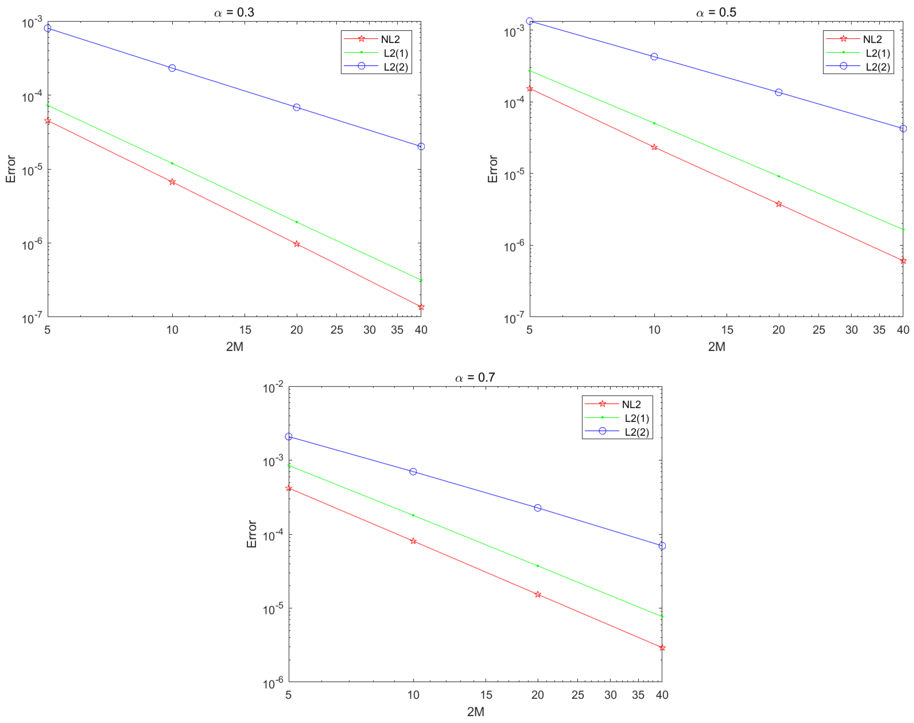
Example 3. 
Consider problem (1) with p ( x , t ) = 2 cos ( x t ) , q ( x , t ) = 1 sin ( x t ) , l = 1 , and T = 1 . The source term f and the initial condition u 0 are selected such that the exact solution of the problem is u ( x , t ) = sin ( π x ) ( t 3 + α + t 2 + 1 ) .
The error of the numerical solutions and the CPU time (seconds) of the three schemes for Example 3 are summarized in Table 8 and Table 9, indicating that the NL2 scheme, the L2(1) scheme, and the L2(2) scheme are stable and convergent. Moreover, the L2(2) scheme often requires the minimal CPU time while the corresponding numerical solution has the largest error. Considering both accuracy and CPU time comprehensively, the NL2 scheme performs the best among the three schemes.
Notably, Table 10 shows that the maximum L 2 -norm error of the numerical solution of the L2(2) scheme is significantly larger than those of other schemes; see also Figure 1. It is interesting that if we modify the first step of the L2(2) scheme, that is, replace it by that of the NL2 scheme (we call it the L2(2)* scheme), then the accuracy of the modified scheme L2(2)* is significantly higher than that of the L2(2) scheme in terms of the maximum L 2 -norm; see Figure 1 and Figure 2. Therefore, the accuracy of the numerical solution at the first time step has a substantial impact on the accuracy of the numerical solution at subsequent time steps. It can also be observed that the numerical solutions obtained by the NL2 scheme are better than those obtained by the L2(1) scheme, the L2(2) scheme, and the L 2 ( 2 ) * scheme.

5. Concluding Remarks

This paper proposes a new L2 (NL2) scheme for time fractional diffusion equations by combining the new L2 scheme with the finite difference method. By analyzing the positive definiteness of the symmetric part of the coefficient matrix B, we prove that the proposed NL2 scheme possesses H 1 -norm stability and achieves the temporal ( 3 α ) th-order accuracy. Numerical experiments are presented to illustrate the accuracy and efficiency of the proposed method. The proposed scheme can be applied to a nonhomogeneous Dirichlet boundary condition directly by updating the right-hand sides of the fully discrete linear systems. On the other hand, although the NL2 scheme can be applied to other types of boundary conditions, e.g., the Neumann boundary condition, the convergence and stability properties need more research. In future work, we will consider applications of the proposed NL2 scheme to other types of boundary conditions and to non-uniform meshes.

Author Contributions

Conceptualization, C.-Y.H. and F.-R.L.; methodology, C.-Y.H. and F.-R.L.; writing—original draft preparation, C.-Y.H.; writing—review and editing, F.-R.L.; visualization, F.-R.L.; supervision, F.-R.L. All authors have read and agreed to the published version of the manuscript.

Funding

This research was supported by the National Natural Science Foundation of China (11771265) and the Guangdong Basic and Applied Basic Research Foundation, Guangdong Province of China (2023A1515030199).

Data Availability Statement

Data sharing is not applicable to this article as no datasets were generated or analyzed during the current study.

Conflicts of Interest

The authors declare no conflicts of interest.

References

  1. Chukbar, K.V. Stochastic transport and fractional derivatives. Zh. Eksp. Toer. Fiz. 1995, 108, 1875–1884. [Google Scholar]
  2. Podlubny, I. Fractional Differential Equations; Academic Press: New York, NY, USA, 1999. [Google Scholar]
  3. Raberto, M.; Scalas, E.; Mainardi, F. Waiting-times and returns in high-frequency financial data: An empirical study. Phys. A Stat. Mech. Appl. 2022, 314, 749–755. [Google Scholar] [CrossRef]
  4. Agrawal, O.P. A general formulation and solution scheme for fractional optimal control problems, Nonlinear Dynam. Zh. Eksp. Toer. Fiz. 2004, 38, 191–206. [Google Scholar]
  5. Benson, D.A.; Wheatcraft, S.W.; Meerschaert, M.M. Application of a fractional advection-dispersion equation. Water Resour. Res. 2006, 36, 1403–1412. [Google Scholar] [CrossRef]
  6. Meerschaert, M.M.; Tadjeran, C. Finite difference approximations for fractional advection-dispersion flow equations. J. Comput. Appl. Math. 2004, 172, 65–77. [Google Scholar] [CrossRef]
  7. Oldham, K.B. Fractional differential equations in electrochemistry. Adv. Eng. Softw. 2010, 41, 9–12. [Google Scholar] [CrossRef]
  8. Ahmad, T.; Sulaiman, M.; Bassir, D.; Alshammari, F.S.; Laouini, G. Enhanced numerical solutions for fractional PDEs using Monte Carlo PINNs coupled with cuckoo search optimization. Fractal Fract. 2025, 9, 225. [Google Scholar] [CrossRef]
  9. Sun, Z.; Wu, X. A fully discrete difference scheme for a diffusion-wave system. Appl. Numer. Math. 2006, 56, 193–209. [Google Scholar] [CrossRef]
  10. Lin, Y.; Xu, C. Finite difference/spectral approximations for the time-fractional diffusion equation. J. Comput. Phys. 2007, 225, 1533–1552. [Google Scholar] [CrossRef]
  11. Zhang, Y.; Sun, Z. Alternating direction implicit schemes for the two-dimensional fractional sub-diffusion equation. J. Comput. Phys. 2011, 230, 8713–8728. [Google Scholar] [CrossRef]
  12. Sun, H.; Chen, W.; Li, C.; Chen, Y. Finite difference schemes for variable-order time fractional diffusion equation. Internat. J. Bifur. Chaos. 2012, 22, 1250085. [Google Scholar] [CrossRef]
  13. Yan, Y.; Pal, K.; Ford, N.J. Higher order numerical methods for solving fractional differential equations. BIT Numer. Math. 2014, 54, 555–584. [Google Scholar] [CrossRef]
  14. Li, C.K.; Liao, W.Y. Applications of inverse operators to a fractional partial integro-differential equation and several well-known differential equations. Fractal Fract. 2025, 9, 200. [Google Scholar] [CrossRef]
  15. Jiang, S.D.; Zhang, J.W.; Zhang, Q.; Zhang, Z.M. Fast evaluation of the Caputo fractional derivative and its applications to fractional diffusion equations. Commun. Comput. Phys. 2017, 21, 650–678. [Google Scholar] [CrossRef]
  16. Yan, Y.G.; Sun, Z.Z.; Zhang, J.W. Fast evaluation of the Caputo fractional derivative and its applications to fractional diffusion equations: A second-order scheme. Commun. Comput. Phys. 2017, 22, 1028–1048. [Google Scholar] [CrossRef]
  17. Wang, Y.M.; Ren, L. A high-order L2-compact difference method for Caputo-type time-fractional sub-diffusion equations with variable coefficients. Appl. Math. Comput. 2019, 342, 71–93. [Google Scholar] [CrossRef]
  18. Mokhtari, R.; Mostajeran, F. A high order formula to approximate the Caputo fractional derivative. Com. Appl. Math. Comput. 2020, 2, 1–29. [Google Scholar] [CrossRef]
  19. Shen, J.Y.; Li, C.P.; Sun, Z.Z. An H2N2 interpolation for Caputo derivative with order in (1,2) and its application to time-fractional wave equations in more than one space dimension. J. Sci. Comput. 2020, 83, 38. [Google Scholar] [CrossRef]
  20. Alikhanov, A.A.; Huang, C.M. A high-order L2 type difference scheme for the time-fractional diffusion equation. Appl. Math. Comput. 2021, 411, 126545. [Google Scholar] [CrossRef]
  21. Quan, C.Y.; Tang, T.; Yang, J. How to define dissipation-preserving energy for time-fractional phase-field equations. CSIAM Trans. Appl. Math. 2020, 1, 478–490. [Google Scholar] [CrossRef]
  22. Fang, Z.W.; Zhang, J.L.; Sun, H.W. A fast finite volume method for spatial fractional diffusion equations on nonuniform meshes. Comput. Math. Appl. 2022, 1, 478–490. [Google Scholar] [CrossRef]
  23. Quan, C.Y.; Wu, X. H1-norm stability and convergence of an L2-type method on nonuniform meshes for subdiffusion equation. SIAM J. Numer. Anal. 2023, 5, 2106–2132. [Google Scholar] [CrossRef]
  24. Gao, G.H.; Sun, Z.Z.; Zhang, H.W. A new fractional numerical differentiation formula to approximate the Caputo fractional derivative and its applications. J. Comput. Phys. 2014, 259, 33–50. [Google Scholar] [CrossRef]
  25. Alikhanov, A.A. A new difference scheme for the time fractional diffusion equation. J. Comput. Phys. 2015, 280, 424–438. [Google Scholar] [CrossRef]
Figure 1. Maximum L 2 -norm Errors of the NL2 scheme, the L2(1) scheme, and the L2(2) scheme for Example 3.
Fractalfract 09 00325 g001
Figure 2. Maximum L 2 -norm Errors of the NL2 scheme, the L2(1) scheme, and the L 2 ( 2 ) * scheme for Example 3.
Fractalfract 09 00325 g002
Table 1. The error and the temporal convergence order of the NL2 scheme in L 2 norm for different values of α ’s with h τ ( 3 α ) / 2 at t = 1 for Example 1.
τ h α = 0.1 Rateh α = 0.5 Rateh α = 0.9 Rate
1 10 1 29 7.2124 × 10⁻⁵ 1 18 1.8698 × 10⁻⁴ 1 12 4.0492 × 10⁻⁴
1 20 1 78 9.9707 × 10−62.8547 1 43 3.2631 × 10−52.5185 1 24 9.7403 × 10−52.0556
1 40 1 211 1.3624 × 10−62.8716 1 101 5.8759 × 10−62.4734 1 49 2.2654 × 10−52.1042
1 80 1 575 1.8344 × 10−72.8927 1 240 1.0341 × 10−62.5065 1 100 5.3227 × 10−62.0895
1 160 1 1571 2.4575 × 10−82.9000 1 570 1.8214 × 10−72.5052 1 207 1.2244 × 10−62.1201
Table 2. The error and the temporal convergence order of the NL2 scheme in L 2 norm for different values of α ’s with h = 1 / 20 , 000 at t = 1 for Example 1.
τ α = 0.3 Rate α = 0.5 Rate α = 0.7 Rate
1 / 10 2.8823 × 10−67.9598 × 10−61.6006 × 10⁻⁵
1 / 20 4.2708 × 10−72.75461.2356 × 10−62.68762.2845 × 10−62.8086
1 / 40 6.2740 × 10−82.76701.8322 × 10−72.75352.6335 × 10−73.1168
1 / 80 8.8311 × 10−92.82872.5857 × 10−82.82501.6577 × 10−83.9898
Table 3. The error in L 2 norm and the temporal convergence order of the NL2 scheme for different values of α ’s with h τ ( 3 α ) / 2 / 100 at t = 1 for Example 1.
τ α = 0.3 Rate α = 0.5 Rate α = 0.7 Rate
1 / 10 2.8934 × 10−67.9769 × 10−61.6033 × 10⁻⁵
1 / 20 4.2905 × 10−72.75361.2383 × 10−62.68752.2902 × 10−62.8075
1 / 40 6.2889 × 10−82.77031.8386 × 10−72.75172.6406 × 10−73.1165
1 / 80 8.5470 × 10−92.87932.5477 × 10−82.85131.6834 × 10−83.9714
Table 4. The maximum L 2 -norm errors over all time steps and the temporal convergence order of the NL2 scheme for different α ’s with h = 1 / 20000 for Example 1.
τ α = 0.3 Rate α = 0.5 Rate α = 0.7 Rate
1 / 10 2.8823 × 10−67.9598 × 10−61.7616 × 10⁻⁵
1 / 20 4.2708 × 10−72.75461.2358 × 10−62.68733.3407 × 10−62.3987
1 / 40 6.2740 × 10−82.76702.0368 × 10−72.60116.0243 × 10−72.4713
1 / 80 9.1147 × 10−92.78313.3265 × 10−82.61421.0547 × 10−72.5139
Table 5. The error in L 2 norm and the temporal convergence order of the NL2 scheme for different values of α ’s with h τ ( 3 α ) / 2 at t = 1 for Example 2.
τ h α = 0.1 Rateh α = 0.5 Rateh α = 0.9 Rate
1 10 1 29 1.1025 × 10⁻³ 1 18 2.7464 × 10⁻³ 1 12 5.7111 × 10⁻³
1 20 1 78 1.5262 × 10−42.8528 1 43 4.8277 × 10−42.5081 1 24 1.4267 × 10−32.0011
1 40 1 211 2.0860 × 10−52.8711 1 101 8.7485 × 10−52.4642 1 49 3.4056 × 10−42.0667
1 80 1 575 2.8090 × 10−62.8926 1 240 1.5483 × 10−52.4984 1 100 8.1394 × 10−52.0649
1 160 1 1571 3.7630 × 10−72.9001 1 570 2.7425 × 10−62.4971 1 207 1.8931 × 10−52.1042
Table 6. The error in the L 2 norm and the temporal convergence order of the NL2 scheme for different values of α ’s with h = 1 / 20 , 000 at t = 1 for Example 2.
τ α = 0.3 Rate α = 0.5 Rate α = 0.7 Rate
1 / 10 4.3775 × 10−61.6118 × 10−54.3291 × 10⁻⁵
1 / 20 6.6164 × 10−72.72602.5993 × 10−62.63256.8838 × 10−62.6528
1 / 40 9.9946 × 10−82.72684.0264 × 10−72.69069.9279 × 10−72.7936
1 / 80 1.6392 × 10−82.60816.1559 × 10−82.70941.3598 × 10−72.8681
Table 7. The maximum L 2 -norm errors over all time steps and the temporal convergence order of the NL2 scheme for different α ’s with h = 1 / 20 , 000 for Example 2.
τ α = 0.3 Rate α = 0.5 Rate α = 0.7 Rate
1 / 10 4.3775 × 10−61.6118 × 10−54.3291 × 10⁻⁵
1 / 20 6.6164 × 10−72.72602.5993 × 10−62.63257.6302 × 10−62.5043
1 / 40 9.9946 × 10−82.72684.0264 × 10−72.69061.4661 × 10−62.3797
1 / 80 1.6392 × 10−82.60816.1559 × 10−82.70942.7864 × 10−72.3955
Table 8. Comparison of errors and CPU times of NL2 scheme, L2(1) scheme, and scheme L2(2) with different α ’s for h τ ( 3 α ) / 2 / 10 at t = 1 for Example 3.
NL2L2(1)L2(2)
α τ Error CPU Error CPU Error CPU
0.3 1 / 10 6.9936 × 10−50.049.7721 × 10−50.057.1219 × 10−50.03
1 / 20 1.0504 × 10−50.051.5792 × 10−50.061.0540 × 10−50.05
1 / 40 1.5595 × 10−60.272.5157 × 10−60.331.5625 × 10−60.26
1 / 80 2.2928 × 10−72.333.9698 × 10−73.982.3239 × 10−73.05
1 / 160 3.4675 × 10−828.746.1642 × 10−839.533.5997 × 10−838.84
0.5 1 / 10 1.9262 × 10−40.033.1207 × 10−40.032.6041 × 10−40.02
1 / 20 3.0226 × 10−50.045.7474 × 10−50.044.5928 × 10−50.04
1 / 40 4.5264 × 10−60.191.0411 × 10−50.248.0600 × 10−60.16
1 / 80 6.4677 × 10−71.431.8689 × 10−62.391.4136 × 10−61.49
1 / 160 8.8360 × 10−813.443.3283 × 10−726.492.4905 × 10−718.01
0.7 1 / 10 4.1540 × 10−40.029.1721 × 10−40.028.4960 × 10−40.02
1 / 20 5.7824 × 10−50.031.9353 × 10−40.041.7628 × 10−40.03
1 / 40 6.3461 × 10−60.124.0095 × 10−50.143.6114 × 10−50.09
1 / 80 3.5028 × 10−70.818.2304 × 10−60.797.3586 × 10−60.78
1 / 160 8.3050 × 10−86.291.6812 × 10−66.521.4960 × 10−68.93
Table 9. Comparison of errors and CPU times of the NL2 scheme, the L2(1) scheme, and the scheme L2(2) with different α ’s for h = 1 / 20 , 000 at t = 1 for Example 3.
NL2L2(1)L2(2)
α τ Error CPU Error CPU Error CPU
0.3 1 / 10 4.5219 × 10−59.317.3020 × 10−511.354.6505 × 10−56.79
1 / 20 6.6985 × 10−614.191.1988 × 10−516.266.7341 × 10−614.45
1 / 40 9.7189 × 10−733.191.9264 × 10−631.849.7346 × 10−730.39
1 / 80 1.3681 × 10−763.463.1677 × 10−766.011.3761 × 10−778.20
0.5 1 / 10 1.5383 × 10−46.812.7330 × 10−49.362.2165 × 10−46.67
1 / 20 2.3350 × 10−514.205.0605 × 10−517.383.9059 × 10−512.86
1 / 40 3.3090 × 10−635.889.1956 × 10−634.616.8450 × 10−635.24
1 / 80 4.4393 × 10−767.471.6661 × 10−680.281.2121 × 10−671.37
0.7 1 / 10 3.5503 × 10−47.458.5687 × 10−49.797.8928 × 10−46.46
1 / 20 4.5470 × 10−514.701.8119 × 10−419.661.6396 × 10−413.26
1 / 40 3.8266 × 10−644.723.7582 × 10−549.593.3610 × 10−526.25
1 / 80 1.8281 × 10−783.567.7254 × 10−689.106.8438 × 10−657.68
Table 10. Comparison of the maximum L 2 -norm errors over all time steps and the temporal convergence order of the NL2, L2(1), and L2(2) schemes for different α ’s with h = 1 / 20 , 000 for Example 3.
NL2L2(1)L2(2)
α τ Error Rate Error Rate Error Rate
0.3 1 / 10 4.5219 × 10−57.2782 × 10−58.0126 × 10⁻⁴
1 / 20 6.6985 × 10−62.75501.1948 × 10−52.60692.3188 × 10−41.7889
1 / 40 9.7189 × 10−72.78501.9197 × 10−62.63776.8228 × 10−51.7649
1 / 80 1.3681 × 10−72.82863.1558 × 10−72.60482.0150 × 10−51.7596
0.5 1 / 10 1.5383 × 10−42.7177 × 10−41.3361 × 10⁻³
1 / 20 2.3350 × 10−52.71985.0317 × 10−52.43324.2579 × 10−41.6498
1 / 40 3.7704 × 10−62.63069.1553 × 10−62.46041.3549 × 10−41.6520
1 / 80 6.0767 × 10−72.63341.6565 × 10−62.46444.2353 × 10−51.6776
0.7 1 / 10 4.2006 × 10−48.4973 × 10−42.0872 × 10⁻³
1 / 20 8.0713 × 10−52.37971.7966 × 10−42.24177.0047 × 10−41.5752
1 / 40 1.5332 × 10−52.39633.7263 × 10−52.26952.2659 × 10−41.6283
1 / 80 2.9245 × 10−62.39037.6597 × 10−62.28246.9574 × 10−51.7034
Disclaimer/Publisher’s Note: The statements, opinions and data contained in all publications are solely those of the individual author(s) and contributor(s) and not of MDPI and/or the editor(s). MDPI and/or the editor(s) disclaim responsibility for any injury to people or property resulting from any ideas, methods, instructions or products referred to in the content.

