Modification to an Auxiliary Function Method for Solving Space-Fractional Stochastic Regularized Long-Wave Equation

Abstract

This study aims to explore the effect of spatial-fractional derivatives and the multiplicative standard Wiener process on the solutions of the stochastic fractional regularized long-wave equation (SFRLWE) and contribute to its analysis. We introduce a new systematic method that combines the auxiliary function method with the complete discriminant polynomial system. This method proves to be effective in discovering precise solutions for stochastic fractional partial differential equations (SFPDEs), including special cases. Applying this method to the SFRLWE yields new exact solutions, offering fresh insights. We investigated how noise affects stochastic solutions and discovered that more intense noise can result in flatter surfaces. We note that multiplicative noise can stabilize the solution, and we show how fractional derivatives influence the dynamics of noise. We found that the noise strength and fractional derivative affect the width, amplitude, and smoothness of the obtained solutions. Additionally, we conclude that multiplicative noise impacts and stabilizes the behavior of SFRLWE solutions.

1. Introduction

Nonlinear partial differential equations (NLPDEs) play a vital role in numerous scientific and engineering disciplines, modeling complex dynamical phenomena such as diffusion, heat transfer, biological systems, fluid dynamics, renewable energy, and communication systems. Modern research emphasizes both their mathematical foundations and their significant applications in fields like physics [1,2,3,4,5]. NLPDEs have been generalized into different classes. The first class is fractional partial differential equations (FPDEs), a set of differential equations that include derivatives of fractional (non-integer) order with respect to the space variables, time, or both. Such derivatives are frequently employed as a modeling tool to improve accuracy in applications governed by differential equations. There are several definitions of fractional derivatives, including conformable derivatives and Caputo–Fabrizio derivatives. For more types of fractional derivatives, see e.g., ref. [6]. Each definition has its own characteristics and is suited to different applications. Some traditional properties of integer-order derivatives—such as the quotient rule, chain rule, and product rule—are not satisfied with fractional derivatives. Different strategies and methods have been developed to handle FPDEs, as given in [7,8,9,10,11,12]. The second class is stochastic partial differential equations (SPDEs). They are differential equations that incorporate random force terms and coefficients, and can be viewed as an extension to NLPDEs by inserting stochastic terms as perturbations. SPDEs are widely used in numerous fields of science [13,14,15]. The third category is the SFPDEs, which join random terms or coefficients with non-integer-order derivatives, thus combining the features of both SPDEs and FPDEs. Several well-known equations have been extended as SFPDEs and analyzed using a diversity of procedures [16,17].

The present work focuses on studying the SFRLWE in the form [17]

$${\mathcal{U}}_t+{\mathbb{T}}_x^p\mathcal{U}-{\displaystyle \frac{{\theta }_1}{2}}\mathcal{U}{\mathbb{T}}_x^p\mathcal{U}-{\theta }_2{\mathbb{T}}_x^{2p}{\mathcal{U}}_t=r(\mathcal{U}-{\theta }_2{\mathbb{T}}_x^{2p}\mathcal{U}){\mathbb{H}}_t,$$

(1)

where ${\mathbb{T}}_x^p\mathcal{U}$ is Jumarie’s modified Riemann–Liouville fractional (JMRLF) derivative of order p, $\mathbb{H}\left(t\right)$ is the standard Wiener process which is commonly referred to as Brownian motion [18], ${\mathbb{H}}_t={\displaystyle \frac{\partial \mathbb{H}}{\partial t}}$, and r is the noise strength. Here, $\mathcal{U}$ is wave function amplitude, t denotes the time, and x refers to the space variable. The parameters ${\theta }_2,{\theta }_1$ are free constants that regulate the dispersive and nonlinear influences, respectively. Equation (1) extends several partial differential equations. In particular, when $p=1,r=0$, Equation (1) takes the classical form

$${\mathcal{U}}_t+{\mathcal{U}}_x-{\displaystyle \frac{{\theta }_1}{2}}\mathcal{U}{\mathcal{U}}_x-{\theta }_2{\mathcal{U}}_{xxt}=0.$$

(2)

Equation (2) refines the long-wave equation by introducing a regularization term to model wave dispersion and enhance the wave propagation modeling accuracy. If ${\theta }_2=1$ and ${\theta }_1=0$, then Equation (2) reduces to a linear wave equation characterizing the waves with small amplitudes. When ${\theta }_2=1$ and ${\theta }_1>0$, it exhibits nonlinear behavior, implying that the amplitude of the wave can vary as it propagates. If ${\theta }_2>1$, it demonstrates dispersive behavior, allowing the wave to change its shape during propagation as a result of the variation in wave velocity with frequency. To the best of our knowledge, Equation (1) was first introduced in [17], where bifurcation theory was used to construct some solutions. The deterministic version of Equation (1), i.e., when $r=0$, has been investigated by several researchers who applied various approaches to find exact solutions. For example, Islam et al. [19], Aminikhah et al. [20], Abdel-Salam and Yousif [21], Korkmaz et al. [22], Jhangeer et al. [23], Güner and Eser [24], Maarouf et al. [25], Naeem et al. [26], etc.

Obtaining solutions to SFPDEs numerically or analytically is not an easy task and requires the use of complicated methods. This motivated us to introduce a systematic process that combines the auxiliary function method with the complete discriminate polynomial system. This method is applicable to a wide class of partial deferential equations and their extensions to FPDEs and SPDEs. To demonstrate the use of the method, we apply it to Equation (1) to drive new solutions. We also discuss and provide a graphical illustration of the influences of fractional derivative and noise intensity.

This paper is structured as follows: Section 2 introduces concepts related to JMRLF derivatives and the standard Wiener process. Section 3 presents the proposed method, which extends the auxiliary function method by incorporating the use of the complete discriminant polynomial system. In Section 4, the effectiveness of the proposed method is shown by deriving new solutions to the SFRLWE. Section 5 provides graphical representations of some obtained solutions and analyzes the individual effects of the fractional derivative and noise strength on these solutions. Finally, Section 6 summarizes the main findings.

2. Preliminaries

To make the paper self-contained, we start by providing an overview of the Wiener process and the JMRLF derivative of order $\nu$.

Fractional derivatives are widely studied due to their versatility in modeling complicated phenomena. Operators like Caputo, Caputo–Fabrizio, and Riemann–Liouville derivatives [6] enable precise representation of memory effects and non-locality, with applications spanning physics, finance, biology, and materials science. Their unique capacity to describe fractional-dimension systems makes them essential tools for analyzing diverse physical phenomena.

Definition 1 

([27]). Let $W:\mathbb{R}\to \mathbb{R}$ be a function, and $\nu \in \mathbb{R}$. The JMRLF derivative of W of order ν is given by

$${\mathbb{T}}_{\tau }^{\nu }\left(W\right)\left(\tau \right)=\left\{\begin{array}{cc}{\displaystyle \frac{1}{\mathsf{\Gamma }(-\nu )}}{\displaystyle \frac{d}{d\tau }}{\int }_0^{\tau }{(\tau -s)}^{-\nu -1}[W\left(s\right)-W\left(0\right)]ds,\hfill & \nu <0\hfill \\ \\ {\displaystyle \frac{1}{\mathsf{\Gamma }(1-\nu )}}{\displaystyle \frac{d}{d\tau }}{\int }_0^{\tau }{(\tau -s)}^{-\nu }[W\left(s\right)-W\left(0\right)]ds,\hfill & 0<\nu <1\hfill \\ \\ {\left(W^{\left(n\right)}\left(\tau \right)\right)}^{(\nu -n)},\hfill & n\le \nu <n+1,n\ge 1,\hfill \end{array}\right.$$

(3)

where $\mathsf{\Gamma }(·)$ is the Euler Gamma function given by

$$\mathsf{\Gamma }\left(z\right)={\int }_0^{\infty }{t}^{z-1}{e}^t\mathrm{d}t,$$

and z is complex number with $\mathrm{Re}z>0$ [6].

The JMRLF derivative has the following properties, which will be used in the subsequent analysis.

$$\begin{array}{cc}\hfill \left(a\right)& {\mathbb{T}}_{\tau }^{\nu }\left({\tau }^s\right)={\displaystyle \frac{\mathsf{\Gamma }(1+s)}{\mathsf{\Gamma }(1+s-\nu )}}{t}^{s-\nu }\hfill \\ \\ \hfill \left(b\right)& {\mathbb{T}}_{\tau }^{\nu }W\left(V\left(\tau \right)\right)={\displaystyle \frac{\mathrm{d}W\left(V\right(\tau \left)\right)}{\mathrm{d}V}}{\mathbb{T}}_{\tau }^{\nu }V\left(\tau \right),whereV:\mathbb{R}\to \mathbb{R}.\hfill \end{array}$$

The standard Wiener process, also known as Brownian motion, is one of the most fundamental stochastic processes in probability theory and stochastic analysis. It was originally introduced to model the random motion of particles suspended in a fluid (Brownian motion) [28], but has become a key tool for modeling randomness across various fields, including biology, physics, engineering, and finance [18,29]. In the context of SPDEs, the Wiener process provides a rigorous mathematical representation of white noise, capturing external randomness in time-dependent systems.

Definition 2 

([30]). A stochastic process ${\left\{\mathbb{H}\left(t\right)\right\}}_{t\ge 0}$ is considered a standard Wiener process if

1. 

$\mathbb{H}\left(0\right)=0$;

2. 

$\mathbb{H}\left(t\right)$ is a continuous function for $t\ge 0$;

3. 

For $t_3<t_2<t_1,$$\mathbb{H}\left(t_1\right)-\mathbb{H}\left(t_2\right)$ and $\mathbb{H}\left(t_2\right)-\mathbb{H}\left(t_3\right)$ are independent;

4. 

For $t_2<t_1$, $\mathbb{H}\left(t_1\right)-\mathbb{H}\left(t_2\right)$ is normally distributed with a mean of zero and a variance of $t_1-t_2$.

Lemma 1 

([30]). Let ${\left\{\mathbb{H}\right\}}_{t\ge 0}$ be a standard Wiener process, then $\mathbb{E}\left(e^{r\mathbb{H}\left(t\right)}\right)=e^{r^{2}t/2}$, where $\mathbb{E}(·)$ is the expectation operator.

3. Methodology

This section introduces a modification of the auxiliary function method through the use of the complete discriminant polynomial systems. We consider a certain class of SFPDEs of the form

$${\mathcal{U}}_t+\sum _{j=1}^l\left(A_j{\mathbb{T}}_x^{jp}\mathcal{U}+B_j{\mathbb{T}}_x^{jp}{\mathcal{U}}_t\right)=r\left(\mathcal{U}+\sum _{j=1}^q{C}_j{\mathbb{T}}_x^{jp}\mathcal{U}\right){\mathbb{H}}_t,$$

(4)

where ${\mathbb{T}}^{jp}$ denotes the JMRLF derivative of order $jp$, r represents the noise strength, $\mathbb{H}\left(t\right)$ is a standard Wiener process, $A_j,B_j,C_j$ are functions in $\mathcal{U}$, and $l,q$ are positive integers. Following [31,32], the solution of Equation (4) is assumed to be in the form of

$$\mathcal{U}(x,t)=M\left(\xi \right)e^{r\mathbb{H}\left(t\right)-{\displaystyle \frac{r^2}{2}}t},\xi ={\displaystyle \frac{k{x}^p}{\Gamma (p+1)}}+\omega t,$$

(5)

where $k,\omega$ are arbitrary constants and $M\left(\xi \right)$ is a real valued function. Substituting the expression (5) into Equation (4) and taking into account Lemma 1, we obtain a reduced equation in the form

$$\mathcal{O}(M,M^{\prime },M^{″},\dots )=0,$$

(6)

where ′ represents the derivative with respect to $\xi$. We will assume that Equation (6) has the solution

$$M\left(\xi \right)=\sum _{i=0}^{\eta }{b}_{i}g{\left(\xi \right)}^i,$$

(7)

where $b_i$ for $i=0,1,\dots ,\eta$ are constants to be computed. Here $\eta \in \mathbb{N}$ is found by equating the highest-order derivative term and the highest power of the nonlinear term in the reduced Equation (6). The function $g\left(\xi \right)$ is a solution of the first-order differential equation

$$g^{\prime }=\sqrt{{\mathcal{F}}_3\left(g\right)},$$

(8)

where

$${\mathcal{F}}_3\left(g\right)=\mu (g^3+a_{1}g+a_0),$$

(9)

and $\mu$, $a_i,i=1,2$ are arbitrary real constants. Notice, the term $g^2$ does not occur in the polynomial ${\mathcal{F}}_3$ since it can usually be removed by a simple transformation. Hence, the problem of finding a solution of the reduced Equation (6), or equivalently, the main Equation (4), reduces to finding all the possible solutions to Equation (8). The variable separation in Equation (8) provides

$$\mathrm{d}\xi ={\displaystyle \frac{\mathrm{d}g}{\sqrt{\mu (g^3+a_{1}g+a_0)}}}.$$

(10)

To integrate (10), we need to determine the types of the roots of the polynomial ${\mathcal{F}}_3\left(g\right)$. We will use the complete discriminate polynomial system for the polynomial ${\mathcal{F}}_3\left(g\right)$ [33]. Taking

$$\Delta =-\left({\displaystyle \frac{a_0^2}{4}}+{\displaystyle \frac{a_1^3}{27}}\right),$$

(11)

we will have the following four possible cases:

Case A. 

If $\Delta =0$ and $a_1<0$, the polynomial ${\mathcal{F}}_3$ has three real roots, one of which is a double root denoted by $g_1>0$, and the other is a simple root whose value is $-2g_1$. Thus, we obtain that ${\mathcal{F}}_3=\mu {(g-g_1)}^2(g+2g_1)$. We consider two possible cases based on whether $\mu$ is a positive or a negative real number.

(a) If $\mu >0$, real solutions exist for g in $(-2g_1,g_1)\cup (g_1,\infty )$. For $g\in (-2g_1,g_1)$, if we assume $g\left(0\right)=-2g_1$, then integrating (10) yields

$$g\left(\xi \right)=-2g_1+g_1{\tanh }^2\left({\displaystyle \frac{\sqrt{\mu g_1}}{2}}\xi \right).$$

(12)

while $g\in (g_1,\infty )$ if we assume $g\left(0\right)=\infty$, the integration of (10) gives the solution

$$g\left(\xi \right)=3g_1{\coth }^2\left({\displaystyle \frac{\sqrt{3\mu g_1}}{2}}\xi \right)-2g_1.$$

(13)

(b) When $\mu <0$, the real solution exists for $g\in (-\infty ,-2g_1)$. Assuming $g\left(0\right)=-2g_1$, integrating both sides of (10) gives

$$g\left(\xi \right)=3g_1{\tan }^2\left({\displaystyle \frac{\sqrt{-3\mu g_1}}{2}}\xi \right)-2g_1.$$

(14)

Case B. 

If $\Delta =0$ and $a_1=0$, then the polynomial (9) has a triple root at the origin, and the function ${\mathcal{F}}_3\left(g\right)$ takes the form ${\mathcal{F}}_3=\mu g^3$. When $\mu >0$, we assume that $g\left(0\right)=\infty$. The integration of Equation (10) yields

$$g\left(\xi \right)={\displaystyle \frac{4}{\mu \xi }}.$$

(15)

Similarly, if $\mu <0$, and if we assume $g\left(0\right)=-\infty$ and integrate both sides of Equation (10), we arrive at the same solution (15).

Case C. 

If $\Delta >0$ and $a_1<0$, then the polynomial in (9) has three real roots, $g_2$, $g_3$, and $-(g_2+g_3)$, and it is assumed that $0<g_2<g_3$. Thus, ${\mathcal{F}}_3$ can be expressed as ${\mathcal{F}}_3=\mu (g-g_2)(g-g_3)(g+g_2+g_3)$. We analyze the following two cases:

(a) When $\mu$ is positive, real solutions exist if $g\in (-g_2-g_3,g_2)\cup (g_3,\infty )$. For $g\in (-g_2-g_3,g_2)$, and assuming $g\left(0\right)=-g_2-g_3$, the integration of Equation (10) yields

$$g\left(\xi \right)=g_3-g_2+(2g_2+g_3){\mathrm{sn}}^2\left({\displaystyle \frac{\sqrt{\mu (g_2+2g_3)}}{2}}\xi ,k_1\right),$$

(16)

where $k_1=\sqrt{{\displaystyle \frac{2g_2+g_3}{g_2+2g_3}}}$ and $\mathrm{sn}(u,k)$ indicates the Jacobi elliptic function [34].

For $g\in (g_3,\infty )$ and assuming $g\left(0\right)=g_3$, the integration of Equation (10) yields

$$g\left(\xi \right)=g_2+(g_2-g_3){\mathrm{nc}}^2\left({\displaystyle \frac{\sqrt{\mu (g_2+2g_3)}}{2}}\xi ,k_1\right),$$

(17)

where $\mathrm{nc}(u,k)=1/\mathrm{cn}(u,k)$ represents the Jacobi elliptic function [34].

(b) When $\mu$ is negative, real solutions exist if $g\in (g_2,g_3)\cup (-\infty ,-g_2-g_3)$. For $g\in (g_2,g_3)$ and assuming $g\left(0\right)=f_3$, the integration of (10) gives

$$g\left(\xi \right)=g_3-(g_3-g_2){\mathrm{sn}}^2\left({\displaystyle \frac{\sqrt{-\mu (g_2+2g_3)}}{2}}\xi ,k_2\right),$$

(18)

where $k_2=\sqrt{{\displaystyle \frac{g_3-g_2}{g_2+2g_3}}}$. For $g\in (-\infty ,-g_2-g_3)$ and assuming $g\left(0\right)=-\infty$, the integration of (10) yields

$$g\left(\xi \right)=g_3-(g_2+2g_2){\mathrm{ns}}^2\left({\displaystyle \frac{\sqrt{-\mu (g_2+2g_3)}}{2}}\xi ,k_2\right),$$

(19)

where $\mathrm{ns}(u,k)=1/\mathrm{sn}(u,k)$ represents the Jacobi elliptic function [34].

Case D. 

If $\Delta <0$, then the polynomial (9) has one real root $-2g_4$, and two complex conjugate roots, $r=g_4+\mathrm{i}{g}_5$ and $r^{*}=g_4-\mathrm{i}{g}_5$. Thus, ${\mathcal{F}}_3$ can be written as ${\mathcal{F}}_3\left(g\right)=\mu (g+2g_4)(g-r)(g-r^{*})$. We consider the following possible cases:

(a) When $\mu \in {\mathbb{R}}^{+}$, the real solution exists if $g\in (-2g_4,\infty )$. Assuming $g\left(0\right)=-g_4$, the integration of (10) yields

$$g\left(\xi \right)=-A-2g_4+{\displaystyle \frac{2A}{1+\mathrm{cn}(\sqrt{\mu A}\xi ,k_3)}},$$

(20)

where

$$k_3=\sqrt{{\displaystyle \frac{1}{2}}+{\displaystyle \frac{3g_4}{2A}}},A^2=9g_4^2+g_5^2.$$

(21)

(b) When $\mu \in {\mathbb{R}}^{-}$, the real solution exists if $g\in (-\infty ,-2g_4)$. Let $g\left(0\right)=-2g_4$, and the integration of (10) yields

$$g\left(\xi \right)=A-2g_4-{\displaystyle \frac{2A}{1+\mathrm{cn}(\sqrt{-\mu A}\xi ,k_3)}}.$$

(22)

Now, we summarize our proposed method in the following algorithm.

Algorithm

To clarify the applicability of the proposed method, we present its applications through the following Algorithm 1. To obtain all possible solutions for the SPDEs of the form (4), we proceed with the following steps:

Algorithm 1 Procedure for solving the SPDE (4).

1: Input: Stochastic fractional partial differential equation (SFPDE) of the form (4) 2: Output: Exact or approximate analytical solutions 3: Insert the assumed solution form given by (5) into the SPDE (4). 4: Use Lemma 1 to simplify and derive the reduced deterministic Equation (6). 5: Assume a solution for the reduced Equation (6) in the form provided by (7), along with the auxiliary function in (8). 6: Determine the positive integer $\eta \in \mathbb{N}$ by equating the highest-order derivative term with the highest-order nonlinear term in (6). 7: Substitute the assumed solution (7) into (6), using the auxiliary relation (16), to obtain a polynomial in terms of g. 8: Equate all coefficients of powers of g to zero, resulting in a nonlinear algebraic system involving physical and solution parameters. 9: Solve the resulting system using the classified cases in Table 1 for $\mu >0$ and Table 2 for $\mu <0$ to find the corresponding solutions. 10: Return the solution of the reduced Equation (6) and hence the original SFPDE (4).

Table 1. Possible solutions to the reduced Equation (6) when $\mu >0$, and where $k_1=\sqrt{{\displaystyle \frac{2g_2+g_3}{g_2+2g_3}}}$, $k_3=\sqrt{{\displaystyle \frac{1}{2}}+{\displaystyle \frac{3g_4}{2A}}}$, and $A^2=9g_4^2+g_5^2$, and $g_i$, $i=1,2,3$ are the roots to the polynomial (9).

Case	$\mathbf{\Delta }$	${\mathit{a}}_1$	Interval of g for Real Solution	Solution $\mathit{g}\left(\mathit{\xi }\right)$
1.	0	−	$(-2g_1,g_1)$	$-2g_1+g_1{\tanh }^2\left({\displaystyle \frac{\sqrt{\mu g_1}}{2}}\xi \right).$
			$(g_1,\infty )$	$3g_1{\coth }^2\left({\displaystyle \frac{\sqrt{3\mu g_1}}{2}}\xi \right)-2g_1.$
2.	0	0	$(0,\infty )$	${\displaystyle \frac{4}{\mu \xi }}.$
3.	+	−	$(-g_2-g_3,g_2)$	$g_3-g_2+(2g_2+g_3){\mathrm{sn}}^2\left({\displaystyle \frac{\sqrt{\mu (g_2+2g_3)}}{2}}\xi ,k_1\right).$
			$(g_3,\infty )$	$g_2+(g_2-g_3){\mathrm{nc}}^2\left({\displaystyle \frac{\sqrt{\mu (g_2+2g_3)}}{2}}\xi ,k_1\right).$
4.	−	arbitrary	$(-2g_4,\infty )$	$-A-2g_4+{\displaystyle \frac{2A}{1+\mathrm{cn}(\sqrt{\mu A}\xi ,k_3)}}$

Table 1. Possible solutions to the reduced Equation (6) when $\mu >0$, and where $k_1=\sqrt{{\displaystyle \frac{2g_2+g_3}{g_2+2g_3}}}$, $k_3=\sqrt{{\displaystyle \frac{1}{2}}+{\displaystyle \frac{3g_4}{2A}}}$, and $A^2=9g_4^2+g_5^2$, and $g_i$, $i=1,2,3$ are the roots to the polynomial (9).

Case	$\mathbf{\Delta }$	${\mathit{a}}_1$	Interval of g for Real Solution	Solution $\mathit{g}\left(\mathit{\xi }\right)$
1.	0	−	$(-2g_1,g_1)$	$-2g_1+g_1{\tanh }^2\left({\displaystyle \frac{\sqrt{\mu g_1}}{2}}\xi \right).$
			$(g_1,\infty )$	$3g_1{\coth }^2\left({\displaystyle \frac{\sqrt{3\mu g_1}}{2}}\xi \right)-2g_1.$
2.	0	0	$(0,\infty )$	${\displaystyle \frac{4}{\mu \xi }}.$
3.	+	−	$(-g_2-g_3,g_2)$	$g_3-g_2+(2g_2+g_3){\mathrm{sn}}^2\left({\displaystyle \frac{\sqrt{\mu (g_2+2g_3)}}{2}}\xi ,k_1\right).$
			$(g_3,\infty )$	$g_2+(g_2-g_3){\mathrm{nc}}^2\left({\displaystyle \frac{\sqrt{\mu (g_2+2g_3)}}{2}}\xi ,k_1\right).$
4.	−	arbitrary	$(-2g_4,\infty )$	$-A-2g_4+{\displaystyle \frac{2A}{1+\mathrm{cn}(\sqrt{\mu A}\xi ,k_3)}}$

Table 2. Possible solutions to the reduced Equation (6) when $\mu <0$, where $k_2=\sqrt{{\displaystyle \frac{g_3-g_2}{g_2+2g_3}}}$, $k_3=\sqrt{{\displaystyle \frac{1}{2}}+{\displaystyle \frac{3g_4}{2A}}}$, and $A^2=9g_4^2+g_5^2$, and $g_i$, $i=1,2,3$ are the roots to the polynomial (9).

Case	$\mathbf{\Delta }$	${\mathit{a}}_1$	Interval of g for Real Solution	Solution $\mathit{g}\left(\mathit{\xi }\right)$
1.	0	−	$(-\infty ,-2g_1)$	$3g_1{\tan }^2\left({\displaystyle \frac{\sqrt{-3\mu g_1}}{2}}\xi \right)-2g_1.$
2.	0	0	$(-\infty ,0)$	${\displaystyle \frac{4}{\mu \xi }}.$
3.	+	−	$(g_2,g_3)$	$g_3-(g_3-g_2){\mathrm{sn}}^2\left({\displaystyle \frac{\sqrt{-\mu (g_2+2g_3)}}{2}}\xi ,k_2\right).$
			$(-\infty ,-g_2-g_3)$	$g_3-(g_2+2g_3){\mathrm{ns}}^2\left({\displaystyle \frac{\sqrt{-\mu (g_2+2g_3)}}{2}}\xi ,k_2\right).$
4.	−	arbitrary	$(-\infty ,-2g_4)$	$A-2g_4-{\displaystyle \frac{2A}{1+\mathrm{cn}(\sqrt{-\mu A}\xi ,k_3)}}.$

Table 2. Possible solutions to the reduced Equation (6) when $\mu <0$, where $k_2=\sqrt{{\displaystyle \frac{g_3-g_2}{g_2+2g_3}}}$, $k_3=\sqrt{{\displaystyle \frac{1}{2}}+{\displaystyle \frac{3g_4}{2A}}}$, and $A^2=9g_4^2+g_5^2$, and $g_i$, $i=1,2,3$ are the roots to the polynomial (9).

Case	$\mathbf{\Delta }$	${\mathit{a}}_1$	Interval of g for Real Solution	Solution $\mathit{g}\left(\mathit{\xi }\right)$
1.	0	−	$(-\infty ,-2g_1)$	$3g_1{\tan }^2\left({\displaystyle \frac{\sqrt{-3\mu g_1}}{2}}\xi \right)-2g_1.$
2.	0	0	$(-\infty ,0)$	${\displaystyle \frac{4}{\mu \xi }}.$
3.	+	−	$(g_2,g_3)$	$g_3-(g_3-g_2){\mathrm{sn}}^2\left({\displaystyle \frac{\sqrt{-\mu (g_2+2g_3)}}{2}}\xi ,k_2\right).$
			$(-\infty ,-g_2-g_3)$	$g_3-(g_2+2g_3){\mathrm{ns}}^2\left({\displaystyle \frac{\sqrt{-\mu (g_2+2g_3)}}{2}}\xi ,k_2\right).$
4.	−	arbitrary	$(-\infty ,-2g_4)$	$A-2g_4-{\displaystyle \frac{2A}{1+\mathrm{cn}(\sqrt{-\mu A}\xi ,k_3)}}.$

This proposed method has the following attractive features:

(i) 

It results in real solutions for the given SFPDEs which are formulated by integrating the differential form (10) over certain intervals of real wave propagation.

(ii) 

It gives the bounded solutions, which can be obtained by integrating the differential form (10) over bounded intervals.

(iii) 

It enables us to construct all possible solutions. This results in the existence of different intervals of real solutions, all subject to the same conditions on the physical parameters. That is, we can derive different solutions from both mathematical and physical perspectives using the same constraints on the physical parameters. Thus, when $\Delta =0$ and $a_1<0$ (i.e., the first case in Table 1), there are two intervals of real solutions, and both lead to completely different solutions. The first solution is bounded and physically meaningful, while the second is unbounded and has no physical interpretation. Thus, the use of intervals of real solutions is significant and cannot be ignored.

4. Application

In this section, we illustrate the utilization of the proposed method and construct new solutions to the SFRLWE (1) by applying the algorithm. It is worth mentioning that the obtained solutions should be compared with those presented in [17], which utilizes bifurcation theory to construct exact solutions to the SFRLWE (1), in order to highlight their novelty. First, we demonstrate how Equation (1) can be derived from Equation (4). By setting $l=q=2$ in (4), we obtain

$${\mathcal{U}}_t+A_1{\mathbb{T}}_x^p\mathcal{U}+B_1{\mathbb{T}}_x^p{\mathcal{U}}_t+A_2{\mathbb{T}}_x^{2p}\mathcal{U}+B_2{\mathbb{T}}_x^{2p}{\mathcal{U}}_t=r\left(\mathcal{U}+C_1{\mathbb{T}}_x^p\mathcal{U}+C_2{\mathcal{T}}_x^{2p}\mathcal{U}\right){\mathbb{H}}_t.$$

(23)

The Equations (1) and (23) are identical when $A_1=1-{\displaystyle \frac{{\theta }_1}{2}}\mathcal{U},B_2=C_2=-{\theta }_2$, and $A_2=B_1=C_1=0$.

Second, we will apply Algorithm 1. Equation (1) is assumed to have a solution in the form (5). After some computations, we obtain

$$\begin{array}{cc}\hfill {\mathcal{U}}_t& =e^{r\mathbb{H}-{\displaystyle \frac{r^2}{2}}t}\left[\omega M^{\prime }+M\left(r{\mathbb{H}}_t+{\displaystyle \frac{r^2}{2}}-{\displaystyle \frac{r^2}{2}}\right)\right],\hfill \end{array}$$

(24a)

$$\begin{array}{cc}\hfill {\mathbb{T}}_x^p\mathcal{U}& =k{M}^{\prime }{e}^{r\mathbb{H}-{\displaystyle \frac{r^2}{2}}t},{\mathbb{T}}_x^{2p}\mathcal{U}=k^2{M}^{\prime \prime }{e}^{r\mathbb{H}-{\displaystyle \frac{r^2}{2}}t},\hfill \end{array}$$

(24b)

$$\begin{array}{cc}\hfill {\mathbb{T}}_x^{2p}{\mathcal{U}}_t& =k^2{e}^{r\mathbb{H}-{\displaystyle \frac{r^2}{2}}t}\left[\omega M^{\prime \prime \prime }+r{M}^{\prime \prime }{\mathbb{H}}_t\right],\hfill \end{array}$$

(24c)

where $+{\displaystyle \frac{r^2}{2}}M$ in (24a) is Itô correction term. Inserting the expression (24) into Equation (1), we obtain

$${\theta }_{2}k\omega M^{\prime \prime \prime }-(\omega +k)M^{\prime }+{\displaystyle \frac{k{\theta }_1}{2}}M{M}^{\prime }{e}^{r\mathbb{H}}{e}^{-{\displaystyle \frac{r^{2}t}{2}}}=0.$$

(25)

Taking the expectation to both sides of Equation (25), we get

$${\theta }_{2}k\omega M^{\prime \prime \prime }-(\omega +k)M^{\prime }+{\displaystyle \frac{k{\theta }_1}{2}}M{M}^{\prime }\mathbb{E}\left(e^{r\mathbb{H}}\right)e^{-{\displaystyle \frac{r^{2}t}{2}}}=0.$$

(26)

Based on Lemma 1, Equation (26) yields

$${\theta }_{2}k\omega M^{\prime \prime \prime }-(\omega +k)M^{\prime }+{\displaystyle \frac{k{\theta }_1}{2}}M{M}^{\prime }=0.$$

(27)

Integrating both sides with respect to $\xi$ and setting the integration constant to be zero, we get the following reduced equation

$$M^{\prime \prime }+3{\gamma }_1{M}^2-2{\gamma }_{2}M=0,$$

(28)

where ${\gamma }_1$ and ${\gamma }_2$ are new constants introduced for simplicity, replacing the original parameters, and are defined as follows:

$${\gamma }_1={\displaystyle \frac{{\theta }_1}{12{\theta }_2\omega }},{\gamma }_2={\displaystyle \frac{k+\omega }{2{\theta }_2\omega k}}.$$

(29)

In the next step, we assume that the reduced Equation (28) has a solution in the form

$$M\left(\xi \right)=\sum _{i=0}^{\eta }{b}_{i}g{\left(\xi \right)}^i,$$

(30)

where $g\left(\xi \right)$ satisfies (8). In third step, we compute $\eta$ by equating the highest order derivative term $M^{\prime \prime }$ and the highest power of the non-linear term $M^2$. After some calculations, we find

$$O\left(M^{\prime \prime }\right)=\eta +1,O\left(M^2\right)=2\eta .$$

(31)

Thus, we have $\eta =1$ and thus, the solution (30) has the form

$$M\left(\xi \right)=b_0+b_{1}g\left(\xi \right).$$

(32)

Using both Equations (5) and (32), the solution to Equation (1) takes the form

$$\mathcal{U}(x,t)=\left[b_0+b_{1}g\left(\xi \right)\right]e^{r\mathbb{H}\left(t\right)-{\displaystyle \frac{r^2}{2}}t}.$$

(33)

It is evident that when $b_0=0$ and $b_1=1$, the solution (33) reduces to the form presented in [17]. Therefore, the solution given by (33) represents a new and more general result.

Substituting the solution (32) in the reduced Equation (28) and using the Equation (8), we obtain a polynomial in g. By setting the coefficients of all powers of g to zero, we derive the following algebraic system:

$$\left\{\begin{array}{c}3b_1^2{\gamma }_1+{\displaystyle \frac{3}{2}}{b}_1\mu =0,\\ 3{\gamma }_1{b}_0^2-2b_0{\gamma }_2+{\displaystyle \frac{1}{2}}{a}_1{b}_1\mu =0,\\ 2b_1(3{\gamma }_1{b}_0-{\gamma }_2)=0.\end{array}\right.$$

(34)

The only obtained solution to the algebraic system (34) is

$$b_0={\displaystyle \frac{{\gamma }_2}{3{\gamma }_1}},a_1=-{\displaystyle \frac{{\gamma }_2^2}{3{\gamma }_1^2{b}_1^2}},\mu =-2b_1{\gamma }_1.$$

(35)

Substituting the values (35) into the discriminate (11), we get

$$\Delta =-{\displaystyle \frac{a_0^2}{4}}+{\displaystyle \frac{{\gamma }_2^6}{729{\gamma }_1^6{b}_1^6}}.$$

(36)

It is clear that $a_1$ is always negative, and consequently, the relevant cases are Case 1 and Case 3 in both Table 1 and Table 2. We investigate these cases individually.

Case I: 

This case is characterized by $\Delta =0$ which holds when $b_1=\pm {\displaystyle \frac{|{\gamma }_2|}{3|{\gamma }_1|}}\sqrt[3]{{\displaystyle \frac{2}{|a_0|}}}$. Thus, the solution (32) becomes

$$M\left(\xi \right)=b_0\pm {\displaystyle \frac{|{\gamma }_2|}{3|{\gamma }_1|}}\sqrt[3]{{\displaystyle \frac{2}{|a_0|}}}g\left(\xi \right).$$

(37)

Depending on sign of $\mu$, some solutions can be found.

(a) If $\mu >0$, which holds when $b_1\alpha <0$, the relevant case is Case 1 in Table 1. For $g\in (-2g_1,g_1)$, the solution to the reduced Equation (28) is as follows:

$$M\left(\xi \right)=b_0\pm {\displaystyle \frac{|{\gamma }_2|}{3|{\gamma }_1|}}\sqrt[3]{{\displaystyle \frac{2}{|a_0|}}}\left(-2g_1+g_1{\tanh }^2\left({\displaystyle \frac{\sqrt{\mu g_1}}{2}}\xi \right)\right).$$

(38)

Consequently, the obtained solution is new and has the form

$$\mathcal{U}(x,t)=\left[b_0\pm {\displaystyle \frac{|{\gamma }_2|}{3|{\gamma }_1|}}\sqrt[3]{{\displaystyle \frac{2}{|a_0|}}}\left(-2g_1+g_1{\tanh }^2({\displaystyle \frac{\sqrt{\mu g_1}}{2}}({\displaystyle \frac{k{x}^p}{\mathsf{\Gamma }(p+1)}}+\omega t)\right)\right]e^{r\mathbb{H}\left(t\right)-{\displaystyle \frac{r^2}{2}}t}.$$

(39)

If $g\in (g_1,\infty )$, the reduced Equation (28) has the solution

$$g\left(\xi \right)=b0\pm {\displaystyle \frac{|{\gamma }_2|}{3|{\gamma }_1|}}\sqrt[3]{{\displaystyle \frac{2}{|a_0|}}}\left(3g_1{\coth }^2\left({\displaystyle \frac{\sqrt{3\mu g_1}}{2}}\xi \right)-2g_1\right).$$

(40)

Thus, a new solution is obtained in the form

$$\mathcal{U}(x,t)=\left[b_0\pm {\displaystyle \frac{|{\gamma }_2|}{3|{\gamma }_1|}}\sqrt[3]{{\displaystyle \frac{2}{|a_0|}}}\left(3g_1{\coth }^2\left({\displaystyle \frac{\sqrt{3\mu g_1}}{2}}({\displaystyle \frac{k{x}^p}{\mathsf{\Gamma }(p+1)}}+\omega t)\right)-2g_1\right)\right]e^{r\mathbb{H}\left(t\right)-{\displaystyle \frac{r^2}{2}}t}.$$

(41)

(b) Suppose $\mu <0$, which holds when $b_1{\gamma }_1>0$ and it is Case 1 in Table 2. If $g\in (-\infty ,-2g_1)$, then the reduced Equation (28) has a solution of the form

$$g\left(\xi \right)=b_0\pm {\displaystyle \frac{|{\gamma }_2|}{3|{\gamma }_1|}}\sqrt[3]{{\displaystyle \frac{2}{|a_0|}}}\left(3g_1{\coth }^2\left({\displaystyle \frac{\sqrt{3\mu g_1}}{2}}\xi \right)-2g_1\right).$$

(42)

Hence, Equation (1) has a solution in the form

$$\mathcal{U}(x,t)=\left[b_0\pm {\displaystyle \frac{|{\gamma }_2|}{3|{\gamma }_1|}}\sqrt[3]{{\displaystyle \frac{2}{|a_0|}}}\left(3g_1{\coth }^2\left({\displaystyle \frac{\sqrt{3\mu g_1}}{2}}({\displaystyle \frac{k{x}^p}{\mathsf{\Gamma }(p+1)}}+\omega t)\right)-2g_1\right)\right]e^{r\mathbb{H}\left(t\right)-{\displaystyle \frac{r^2}{2}}t}.$$

(43)

Case II: 

Assume $\Delta >0$, which holds if $|b_1|<{\displaystyle \frac{|{\gamma }_2|}{3|{\gamma }_1|}}\sqrt[3]{{\displaystyle \frac{2}{|a_0|}}}$. The solutions are classified based on the sign of $\mu$ as follows:

(a) If $\mu >0$, which satisfies when $b_1{\gamma }_1<0$ and it is Case 3 in Table 1. If $g\in (-g_2-g_3,g_2)$, the solution of the reduced Equation (28) has the form

$$g\left(\xi \right)=b_0+b_1\left\{g_3-g_2+(2g_2+g_3){\mathrm{sn}}^2\left({\displaystyle \frac{\sqrt{\mu (g_2+2g_3)}}{2}}\xi ,k_1\right)\right\}.$$

(44)

Hence, the obtained solution to Equation (1) is new and has the form

$$\begin{array}{cc}\hfill \mathcal{U}(x,t)& =\left[b_0+b_1\left\{g_3-g_2+(2g_2+g_3){\mathrm{sn}}^2\left({\displaystyle \frac{\sqrt{\mu (g_2+2g_3)}}{2}}({\displaystyle \frac{k{x}^p}{\mathsf{\Gamma }(p+1)}}+\omega t),k_1\right)\right\}\right]\hfill \\ \hfill & \times e^{r\mathbb{H}\left(t\right)-{\displaystyle \frac{r^2}{2}}t}.\hfill \end{array}$$

(45)

If $g\in (g_3,\infty )$, the solution of the reduced Equation (28) becomes

$$g\left(\xi \right)=b_0+b_1\left\{g_2+(g_2-g_3){\mathrm{nc}}^2\left({\displaystyle \frac{\sqrt{\mu (g_2+2g_3)}}{2}}\xi ,k_1\right)\right\}.$$

(46)

As a result, the solution to Equation (1) is expressed in the form

$$\begin{array}{cc}\hfill \mathcal{U}(x,t)& =\left[b_0+b_1\left\{g_2+(g_2-g_3){\mathrm{nc}}^2\left({\displaystyle \frac{\sqrt{\mu (g_2+2g_3)}}{2}}({\displaystyle \frac{k{x}^p}{\mathsf{\Gamma }(p+1)}}+\omega t),k_1\right)\right\}\right]\hfill \\ \hfill & \times e^{r\mathbb{H}\left(t\right)-{\displaystyle \frac{r^2}{2}}t}.\hfill \end{array}$$

(47)

The solution (47) is novel solution to Equation (1).

(b) If $\mu <0$, which verifies when $b_1{\gamma }_1<0$, corresponding to Case 3 in Table 2. If $g\in (g_2,g_3)$, then the solution to the reduced equation is

$$g\left(\xi \right)=b_0+b_1\left\{g_3-(g_3-g_2){\mathrm{sn}}^2\left({\displaystyle \frac{\sqrt{-\mu (g_2+2g_3)}}{2}}\xi ,k_2\right)\right\}.$$

(48)

Therefore, the solution to Equation (1) has the form

$$\begin{array}{cc}\hfill \mathcal{U}(x,t)& =\left[b0+b_1\left\{g_3-(g_3-g_2){\mathrm{sn}}^2\left({\displaystyle \frac{\sqrt{-\mu (g_2+2g_3)}}{2}}({\displaystyle \frac{k{x}^p}{\mathsf{\Gamma }(p+1)}}+\omega t),k_2\right)\right\}\right]\hfill \\ \hfill & \times e^{r\mathbb{H}\left(t\right)-{\displaystyle \frac{r^2}{2}}t}.\hfill \end{array}$$

(49)

The solution (49) represents a new solution to Equation (1). If $g\in (-\infty ,-g_2-g_3)$, then the reduced Equation (28) has a solution of the form

$$g\left(\xi \right)=b0+b_1\left\{g_3-(g_2+2g_2){\mathrm{ns}}^2\left({\displaystyle \frac{\sqrt{-\mu (g_2+2g_3)}}{2}}\xi ,k_2\right)\right\}.$$

(50)

Hence, the solution to Equation (1) becomes

$$\begin{array}{cc}\hfill \mathcal{U}(x,t)& =\left[b0+b_1\left\{g_3-(g_2+2g_2){\mathrm{ns}}^2\left({\displaystyle \frac{\sqrt{-\mu (g_2+2g_3)}}{2}}({\displaystyle \frac{k{x}^p}{\mathsf{\Gamma }(p+1)}}+\omega t),k_2\right)\right\}\right]\hfill \\ \hfill & \times e^{r\mathbb{H}\left(t\right)-{\displaystyle \frac{r^2}{2}}t}.\hfill \end{array}$$

(51)

5. Graphical Representation

This section gives graphical representations of some obtained solutions and explores the individual effects of spatial-fractional derivatives and noise strength. We implement numerical simulations in MATLAB [35] to validate some selected solutions and investigate the influence of noise strength and fractional derivative.

Assume that ${\theta }_1=0.1,{\theta }_2=0.4$. With these values, Equation (1) becomes

$${\mathcal{U}}_t+{\mathbb{T}}_x^p\mathcal{U}-0.05\mathcal{U}{\mathbb{T}}_x^p\mathcal{U}-0.4{\mathbb{T}}_x^{2p}{\mathcal{U}}_t=r(\mathcal{U}-0.4{\mathbb{T}}_x^{2p}\mathcal{U}){\mathbb{H}}_t.$$

(52)

Assuming $\omega =2$ and $k=10$ and substituting these values into (29), yields ${\gamma }_1=0.01041666667$ and ${\gamma }_2=0.075$, and substituting Equation (35) gives

$$b_0=2.399999999,a_1=-{\displaystyle \frac{17.27999999}{b_1^2}},\mu =0.02083333334b_1.$$

(53)

Finally, Equation (36) gives

$$\Delta :=-{\displaystyle \frac{a_0^2}{4}}+{\displaystyle \frac{191.1029757}{b_1^6}}.$$

(54)

Note that the constant $a_1$ is always negative, and thus the cases in Table 1 and Table 2 that are corresponding to the solutions depend on $b_1$. We will construct solutions of Equation (52) based on a suitable choice of $a_0$ and $b_1$, as follows:

(a) 

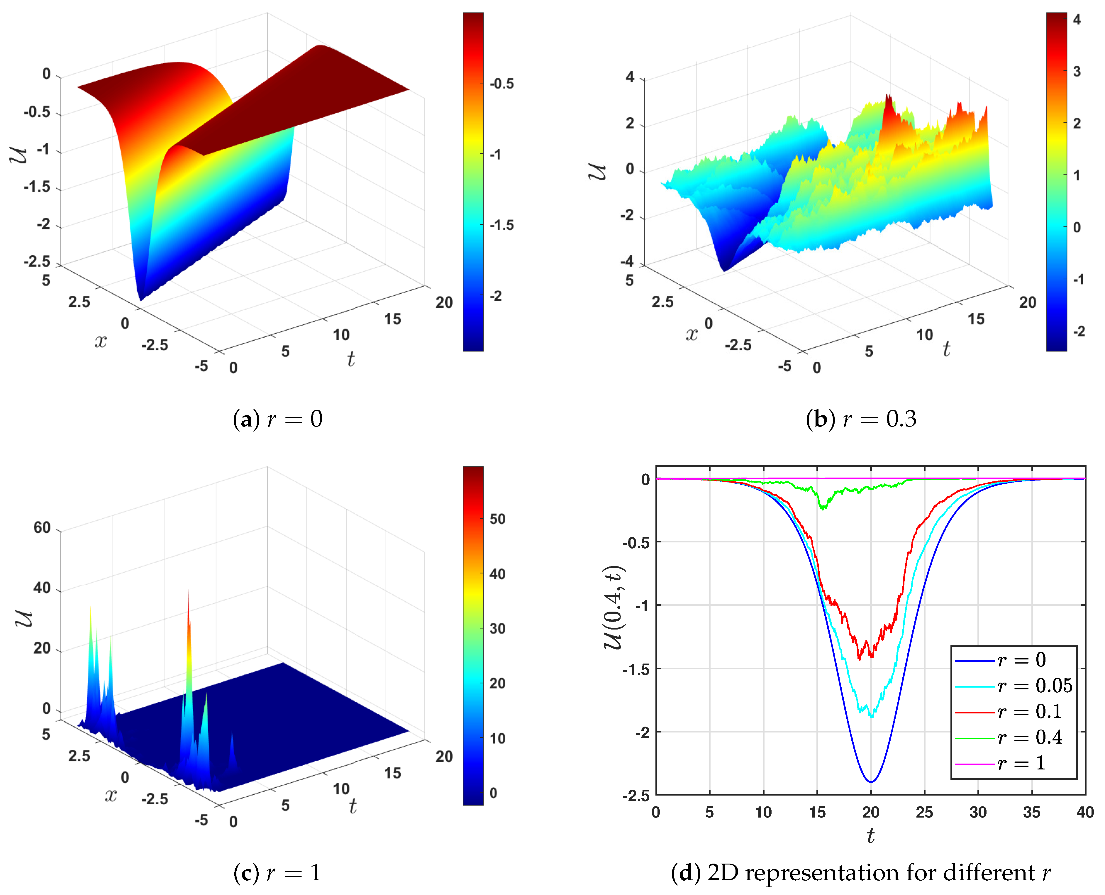
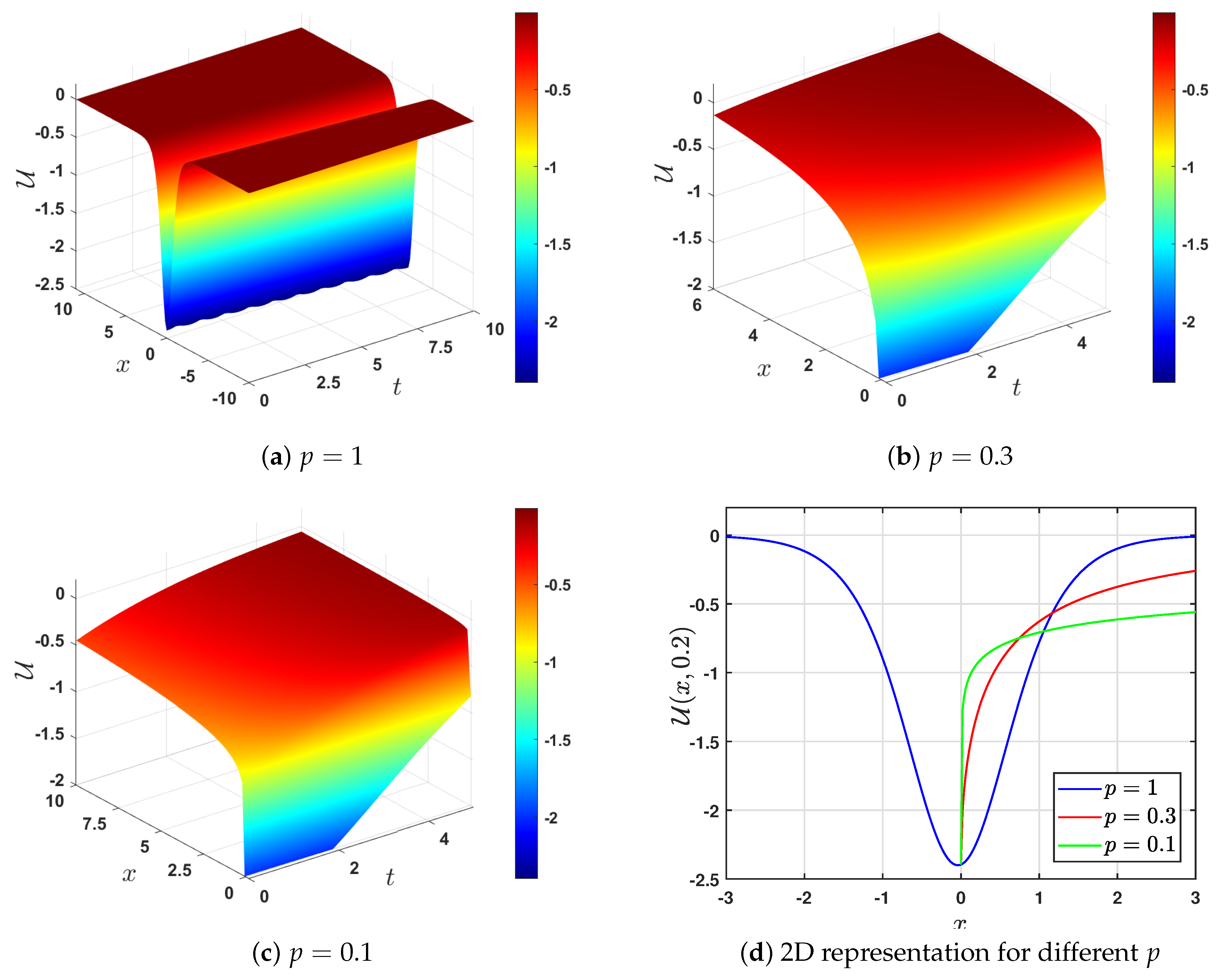
By choosing $a_0=1$ and $b_1=-3.387729703$, we find $\Delta =0$. The roots of the polynomial (9) are $g_1=0.7937005259$ (a double root) and $-2g_1=-1.587401052$ (a simple root), with $\mu =0.06299605250>0$. Therefore, the possible solutions to Equation (52) are (39) and (41), correspondingly. These solutions depend on the intervals of g.

Thus, we have

i. For $g\in (-2g_1,g_1)=(-1.587401052,0.7937005259)$, Equation (52) has a solution of the form

$$\mathcal{U}(x,t)=-2.4{\mathrm{sech}}^2\left({\displaystyle \frac{1.118033988x^p}{\mathsf{\Gamma }\left(p+1\right)}}+0.2236067977t\right)e^{r\mathbb{H}\left(t\right)-{\displaystyle \frac{r^2}{2}}t}.$$

(55)

ii. When $g\in (g_1,\infty )=(0.7937005259,\infty )$, Equation (52) has a solution of the form

$$\begin{array}{cc}\hfill \mathcal{U}(x,t)& =\left[2.381101578{coth}^2\left({\displaystyle \frac{1.936491673x^p}{\mathsf{\Gamma }\left(p+1\right)}}+0.3872983346t\right)-1.587401052\right]\hfill \\ \hfill & \times e^{\rho \mathbb{H}\left(t\right)-{\displaystyle \frac{{\rho }^2}{2}}t}.\hfill \end{array}$$

(56)

Figure 1 illustrates the solution (55) of Equation (52) with integer-order derivatives for different values of the noise strength r. Figure 1a shows that the solution is solitary and smooth in the deterministic case ($r=0$). As the noise strength increases, the surface of the solution loses its smoothness, as shown in Figure 1b. For larger values of noise, the solution becomes flat (planar), as depicted in Figure 1c. Figure 1d shows the 2D representation of the solution (55) with $p=1$ for various values of r. We observe that the amplitude and width of the solution decrease as the noise r increases until the solution ultimately flattens into a line for the highest values of r as shown in pink.

Figure 2 illustrates the effect of the fractional derivative of order p on the solution (55) of Equation (52) in the deterministic case $r=0$. In Figure 2a, the solution (52) is shown to be solitary. As the fractional derivative of order p decreases from one, the solution loses its symmetry. Figure 2d shows the 2D representation of the solution (55) for various values of p. We observe that as p decreases from one, the solution loses its symmetry, its width decreases, and its height remains nearly constant. Furthermore, as p approaches zero, the solution becomes flat.

Figure 2 displays the effect of the fractional derivative of order p on the solution (55) of the Equation (52) in the deterministic case, i.e., when $r=0$. In Figure 2a, it is shown that the solution (52) is solitary and symmetric. As the fractional derivative order p decreases from one, the solution loses its symmetry as shown in Figure 2b,c, its width decreases, and its height remains nearly constant. In Figure 2b, we depict the surface associated with the solution (52). It shows that the surface is symmetric when $p=1$ and becomes asymmetric for $p\in (0,1)$.

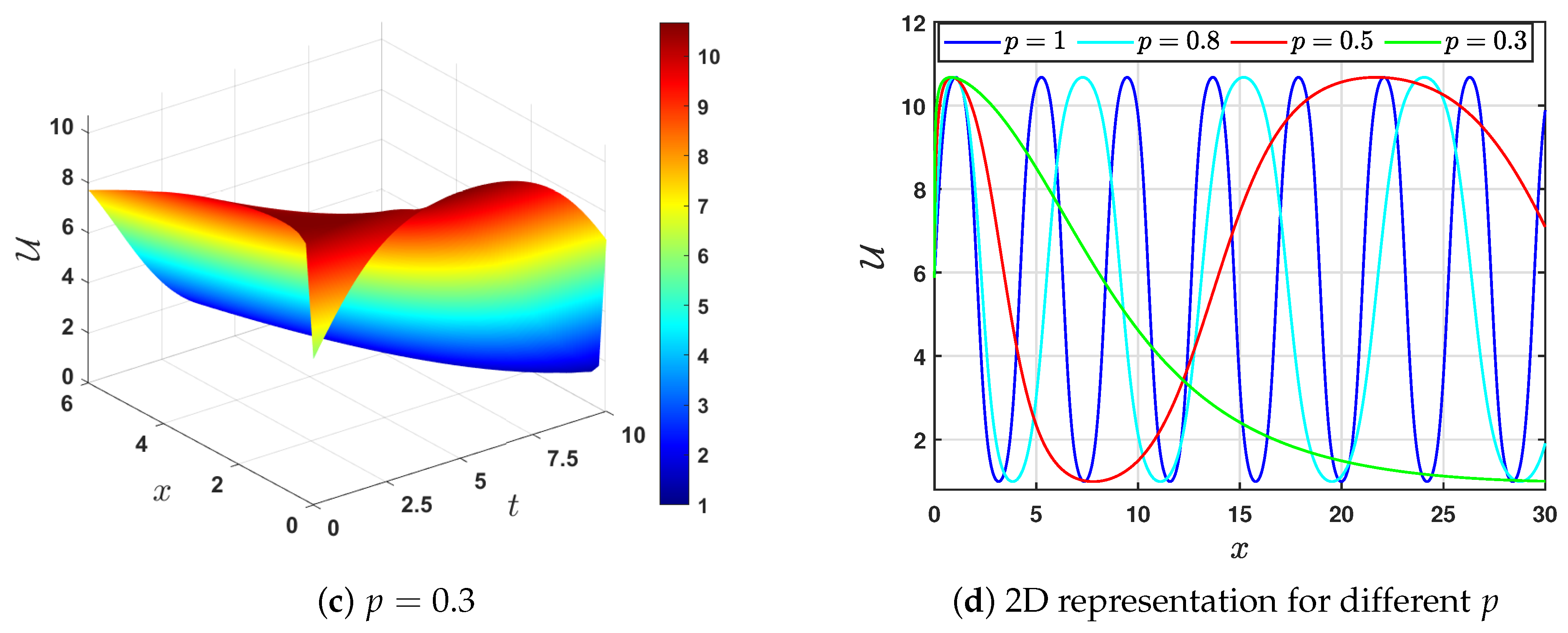
(b) 

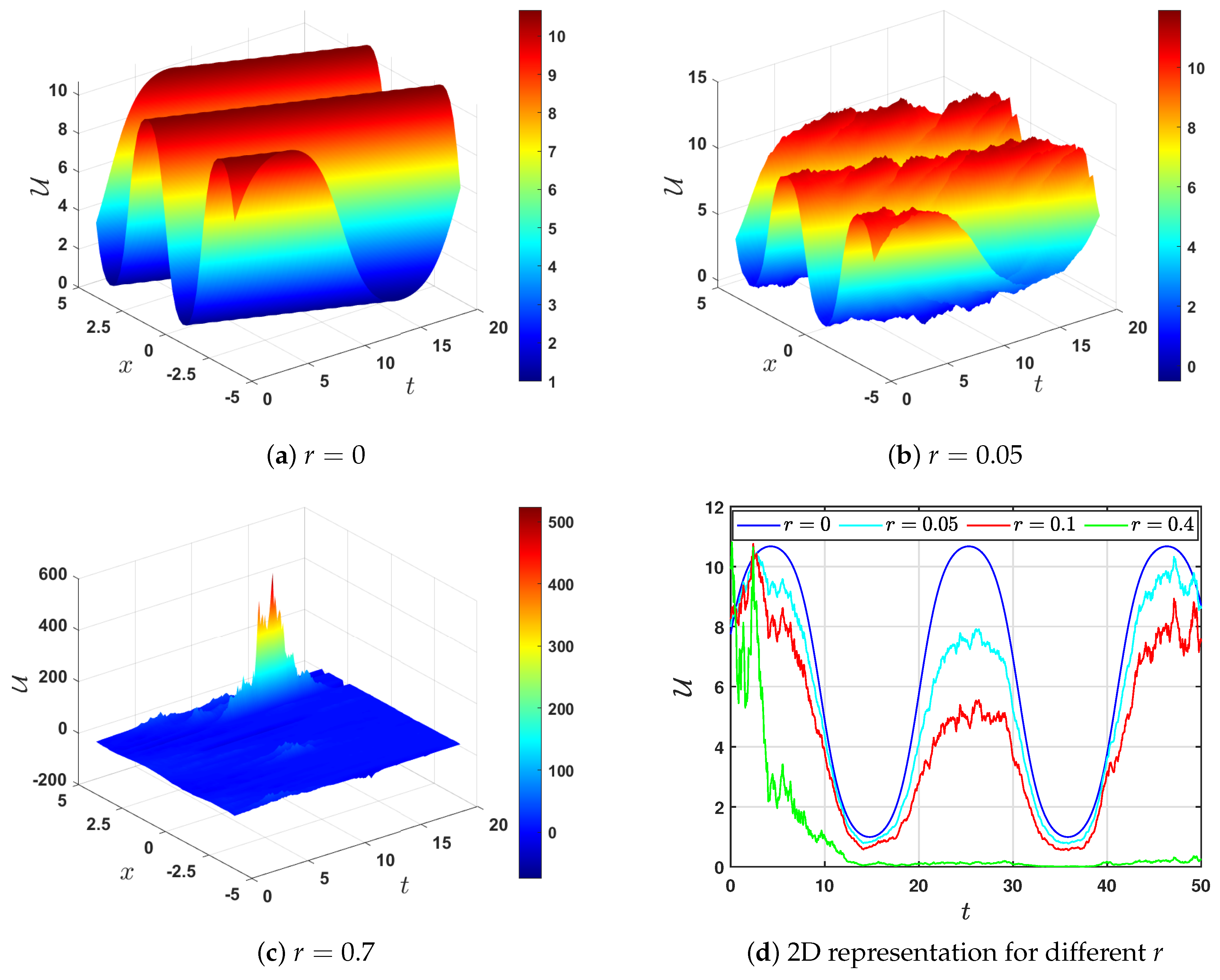
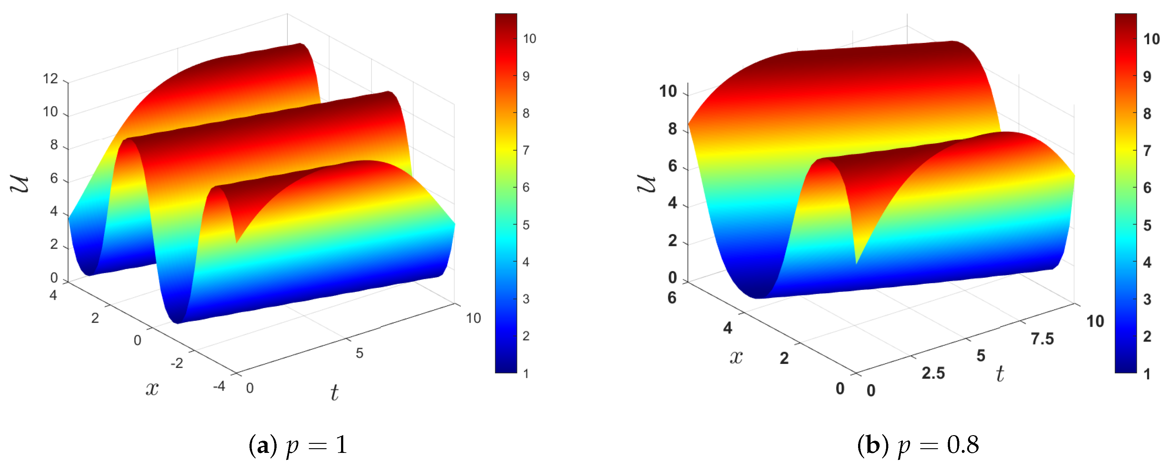
Selecting $a_0=1$ and choosing $b_1\in (-3.023810519,0)\cup (0,3.023810519)$, we find that $\Delta >0$. Hence, the derived solutions of (52) can be constructed by using Case 3 in both Table 1 and Table 2, depending on the sign of $\mu$, which in turn depends on the sign of $b_1$. Therefore, we select two values of $b_1$ and consider them separately as follows.

If we choose $b_1=2$, we find that $\mu >0$, and consequently, we use Case 3 in Table 1. The roots of the polynomial (9) are $g_2=0.2344651543$, $g_3=1.951286112$, and $-g_2-g_3=-2.185751266$. Depending on the intervals of g, we have

i. If $g\in (-g_2-g_3,g_2)=(-2.185751266,1.951286112)$, then Equation (52) has the solution

$$\begin{array}{cc}\hfill \mathcal{U}(x,t)& =\left[5.833641915+4.840432842{\mathrm{sn}}^2\left({\displaystyle \frac{2.075912796x^p}{\mathsf{\Gamma }\left(p+1\right)}}+0.4151825592t,0.7648607575\right)\right]\hfill \\ \hfill & \times e^{\rho \mathbb{H}\left(t\right)-{\displaystyle \frac{{\rho }^2}{2}}t}.\hfill \end{array}$$

(57)

ii. If $g\in (g_3,\infty )=(1.951286112,\infty )$, then Equation (52) has a solution in the form

$$\begin{array}{cc}\hfill \mathcal{U}(x,t)& =\left[0.2344651543-{\displaystyle \frac{1.716820958}{{\mathrm{cn}}^2\left(\frac{2.075912796x^p}{\mathsf{\Gamma }\left(p+1\right)}+0.4151825592t,0.7648607575\right)}}\right]\hfill \\ \hfill & e^{\rho \mathbb{H}\left(t\right)-{\displaystyle \frac{{\rho }^2}{2}}t}.\hfill \end{array}$$

(58)

If we select $b_1=-2$, then $\mu$ is negative and we utilize Table 2 to construct the solutions. Based on the intervals of real wave propagation, we have

i. If $g\in (g_2,g_3)=(0.2344651543,1.951286112)$, then Equation (52) has a solution in the form

$$\begin{array}{cc}\hfill \mathcal{U}(x,t)& =\left[-1.502572225+3.433641916{\mathrm{sn}}^2\left({\displaystyle \frac{2.075912796x^p}{\mathsf{\Gamma }\left(p+1\right)}}+0.4151825592t,0.6441956395\right)\right]\hfill \\ \hfill & \times e^{\rho \mathbb{H}\left(t\right)-{\displaystyle \frac{{\rho }^2}{2}}t}.\hfill \end{array}$$

(59)

ii. If $g\in (-\infty ,-g_2-g_3)=(-\infty ,-2.185751266)$, then Equation (52) has a solution in the form

$$\begin{array}{cc}\hfill \mathcal{U}(x,t)& =\left[-1.502572225+{\displaystyle \frac{8.274074756}{{\mathrm{sn}}^2\left(0.2075912796\left(\frac{10x^p}{\mathsf{\Gamma }\left(p+1\right)}+2t\right),0.6441956395\right)}}\right]\hfill \\ \hfill & \times e^{\rho \mathbb{H}\left(t\right)-{\displaystyle \frac{{\rho }^2}{2}}t}.\hfill \end{array}$$

(60)

In the following, we graphically illustrate the solution (57) and clarify how it is affected by the fractional derivative and noise strength individually.

Figure 3 shows the solution (57) of (52) with integer-order derivatives for different values of the noise strength r. In Figure 3a we show that the solution remains periodic in the deterministic case ($r=0$). However, as the noise increases, the solution becomes rough as shown in Figure 3b. However, as the noise strength increases, the surface represented by the solution becomes rough, as seen in Figure 3b. For larger values of r, the surface flattens after a brief transient phase, as depicted in Figure 3c. In Figure 3d we show a 2D representation of the solution (57) for various values of r. Notably, both the width and amplitude of the solution decrease as the noise strength increases. Furthermore, for sufficiently large r, the amplitude diminishes, and the periodic behavior fades, eventually leading to a flat (planar) solution, as highlighted in green in Figure 3d.

In Figure 4, the impact of the fractional derivative of order p on the solution (57) is shown in deterministic case $(r=0)$. Figure 4a shows that the solution is periodic when $p=1$. However, as p decreases from one, the amplitude of the solution remains nearly unchanged, while its width increases rapidly, as shown in Figure 4b. For smaller values of p, the width of the solution expands even more rapidly, as depicted in Figure 4c, leading to a loss of periodicity. Finally, Figure 4d confirms that while the amplitude remains approximately unchanged, the width of the solution continues to grow significantly as the order of the fractional derivative decreases from one.

6. Conclusions

This parer has two primary objectives. First, we introduce a new systematic approach for solving a broad class of NLPDEs and their extensions—including FPDEs, SPDEs, and SFPDEs. A natural strategy for developing such a method is to refine or extend existing techniques. Here, we propose a novel hybrid method combining the auxiliary function approach with the complete discriminant polynomial system. This combination successfully generates new exact solutions for the SFRLWE, addressing limitations of traditional methods, which often struggle with the nonlinearity, nonlocality, and randomness inherent in SFPDEs. By systematically reducing nonlinear SFPDEs to algebraic forms via auxiliary functions and discriminant analysis, our framework provides a tractable pathway to exact solutions in complex settings (see, e.g., ref. [36,37]). The proposed method has some advantages, as follows:

(i) 

It provides only real solutions for the given SFPDEs and its special cases because these solutions are obtained by integrating the differential form (10) over certain intervals of real wave propagation.

(ii) 

It enables the construction of all possible solutions. This results in the existence of different intervals of real solutions, all subject to the same conditions on the physical parameters. In other words, with the same constraints on the physical parameters, we can derive different solutions. Thus, in the first case in Table 1, when $\Delta =0$ and $a_1<0$, there are two intervals of real solutions, and both lead to completely different solutions from both mathematical and physical viewpoints. The first solution is bounded and physically meaningful, while the second is unbounded, and has no physical interpretation. Therefore, the use of intervals of real solutions is significant and cannot be ignored.

(iii) 

It isolates the bounded solutions, which can be obtained by integrating the differential form (10) over bounded intervals only.

We propose an algorithm to demonstrate the applicability of our method. This method is then used to derive new solutions for the SFRLWE. In comparison to [17], the solutions obtained for the SFRLWE (1) are entirely new. Furthermore, these solutions also represent novel solutions for a special case of Equation (1), as discussed in previous works [19,20,25]. These solutions are graphically illustrated using 2D and 3D representations. Additionally, we analyze separately the impact of the fractional derivative and noise strength on some of these solutions. We observed that changing the order of the spatial-fractional derivative significantly affects the shape of the solution profiles. Lower fractional derivatives result in more dispersed and flattened waveforms, while higher orders preserve sharper wave features, as shown in Figure 4. This behavior arises because fractional spatial derivatives introduce nonlocality, meaning the solution’s evolution at any given point depends on a broader spatial region. As the order decreases, the degree of nonlocality increases, leading to more diffusion-like or dispersive effects. This not only impacts wave speed but also influences the amplitude and overall structure of the solutions. For more details, see, for example, refs. [6,38]. Furthermore, we found that the impact of multiplicative noise varies with its intensity. High-intensity noise tends to dominate the system’s dynamics, causing profile flattening, which means energy dissipation or dispersal, due to excessive stochastic forcing. In contrast, moderate-intensity noise can suppress instabilities by counteracting deterministic nonlinearities, as illustrated in Figure 1. This finding is consistent with previous studies, such as [39,40].

References

- Ilhan, O.A.; Manafian, J. Periodic type and periodic cross-kink wave solutions to the (2+ 1)-dimensional breaking soliton equation arising in fluid dynamics. Mod. Phys. Lett. B 2019, 33, 1950277. [Google Scholar] [CrossRef]
- Ilhan, O.A.; Manafian, J.; Lakestani, M.; Singh, G. Some novel optical solutions to the perturbed nonlinear Schrödinger model arising in nano-fibers mechanical systems. Mod. Phys. Lett. B 2022, 36, 2150551. [Google Scholar] [CrossRef]
- Albalawi, S.M.; Elmandouh, A.A.; Sobhy, M. Integrability and dynamic behavior of a piezoelectro-magnetic circular rod. Mathematics 2024, 12, 236. [Google Scholar] [CrossRef]
- Aljuaidan, A.; Elbrolosy, M.; Elmandouh, A. Nonlinear Wave Propagation for a Strain Wave Equation of a Flexible Rod with Finite Deformation. Symmetry 2023, 15, 650. [Google Scholar] [CrossRef]
- Elmandouh, A. Bifurcation, quasi-periodic, chaotic pattern, and soliton solutions for a time-fractional dynamical system of ion sound and Langmuir waves. Math. Methods Appl. Sci. 2025, 48, 3825–3841. [Google Scholar] [CrossRef]
- Kilbas, A.A.; Srivastava, H.M.; Trujillo, J.J. Theory and Applications of Fractional Differential Equations; North-Holland Mathematical Studies; Elsevier Science Inc.: Amsterdam, The Netherlands, 2006; Volume 204. [Google Scholar]
- Ali, A.I.; Kalim, M.; Khan, A. Solution of fractional partial differential equations using fractional power series method. Int. J. Differ. Equ. 2021, 2021, 6385799. [Google Scholar] [CrossRef]
- Bayrak, M.A.; Demir, A.; Ozbilge, E. A novel approach for the solution of fractional diffusion problems with conformable derivative. Numer. Methods Partial. Differ. Equ. 2023, 39, 1870–1887. [Google Scholar] [CrossRef]
- Bayrak, M.A.; Demir, A.; Ozbilge, E. On the numerical solution of conformable fractional diffusion problem with small delay. Numer. Methods Partial. Differ. Equ. 2022, 38, 177–189. [Google Scholar] [CrossRef]
- Thabet, H.; Kendre, S. Analytical solutions for conformable space-time fractional partial differential equations via fractional differential transform. Chaos Solitons Fractals 2018, 109, 238–245. [Google Scholar] [CrossRef]
- Thabet, H.; Kendre, S.; Peters, J. Advances in solving conformable nonlinear partial differential equations and new exact wave solutions for Oskolkov-type equations. Math. Methods Appl. Sci. 2022, 45, 2658–2673. [Google Scholar] [CrossRef]
- Siddique, I.; Mehdi, K.B.; Jaradat, M.M.; Zafar, A.; Elbrolosy, M.E.; Elmandouh, A.A.; Sallah, M. Bifurcation of some new traveling wave solutions for the time–space M-fractional MEW equation via three altered methods. Results Phys. 2022, 41, 105896. [Google Scholar] [CrossRef]
- Edwards, S.F.; Wilkinson, D. The surface statistics of a granular aggregate. Proc. R. Soc. Lond. Math. Phys. Sci. 1982, 381, 17–31. [Google Scholar]
- Liu, W.; Röckner, M. Stochastic Partial Differential Equations: An Introduction; Springer: Berlin/Heidelberg, Germany, 2015. [Google Scholar]
- Li, Z.; Liu, C. Chaotic pattern and traveling wave solution of the perturbed stochastic nonlinear Schrödinger equation with generalized anti-cubic law nonlinearity and spatio-temporal dispersion. Results Phys. 2024, 56, 107305. [Google Scholar] [CrossRef]
- Elmandouh, A.; Al Nuwairan, M.; El-Dessoky, M. Nonlinear Dynamical Analysis and New Solutions of the Space-Fractional Stochastic Davey—Stewartson Equations for Nonlinear Water Waves. Mathematics 2025, 13, 692. [Google Scholar] [CrossRef]
- Almutairi, B.; Al Nuwairan, M.; Aldhafeeri, A. Exploring the Exact Solution of the Space-Fractional Stochastic Regularized Long Wave Equation: A Bifurcation Approach. Fractal Fract. 2024, 8, 298. [Google Scholar] [CrossRef]
- Oksendal, B. Stochastic Differential Equations: An Introduction with Applications; Springer Science & Business Media: Berlin/Heidelberg, Germany, 2013. [Google Scholar]
- Islam, S.R.; Khan, K.; Akbar, M.A. Exact solutions of unsteady Korteweg-de Vries and time regularized long wave equations. SpringerPlus 2015, 4, 124. [Google Scholar] [CrossRef]
- Aminikhah, H.; Refahi Sheikhani, A.; Rezazadeh, H. Sub-equation method for the fractional regularized long-wave equations with conformable fractional derivatives. Sci. Iran. 2016, 23, 1048–1054. [Google Scholar] [CrossRef]
- Abdel-Salam, E.A.B.; Yousif, E.A. Solution of Nonlinear Space-Time Fractional Differential Equations Using the Fractional Riccati Expansion Method. Math. Probl. Eng. 2013, 2013, 846283. [Google Scholar] [CrossRef]
- Korkmaz, A.; Hepson, O.E.; Hosseini, K.; Rezazadeh, H.; Eslami, M. Sine-Gordon expansion method for exact solutions to conformable time fractional equations in RLW-class. J. King Saud-Univ.-Sci. 2020, 32, 567–574. [Google Scholar] [CrossRef]
- Jhangeer, A.; Muddassar, M.; Kousar, M.; Infal, B. Multistability and dynamics of fractional regularized long wave equation with conformable fractional derivatives. Ain Shams Eng. J. 2021, 12, 2153–2169. [Google Scholar] [CrossRef]
- Güner, Ö.; Eser, D. Exact solutions of the space time fractional symmetric regularized long wave equation using different methods. Adv. Math. Phys. 2014, 2014, 456804. [Google Scholar] [CrossRef]
- Maarouf, N.; Maadan, H.; Hilal, K. Lie symmetry analysis and explicit solutions for the time-fractional regularized long-wave equation. Int. J. Differ. Equ. 2021, 2021, 6614231. [Google Scholar] [CrossRef]
- Naeem, M.; Yasmin, H.; Shah, R.; Shah, N.A.; Nonlaopon, K. Investigation of fractional nonlinear regularized long-wave models via novel techniques. Symmetry 2023, 15, 220. [Google Scholar] [CrossRef]
- Jumarie, G. Modified Riemann-Liouville derivative and fractional Taylor series of nondifferentiable functions further results. Comput. Math. Appl. 2006, 51, 1367–1376. [Google Scholar] [CrossRef]
- Einstein, A. Über die von der molekularkinetischen Theorie der Wärme geforderte Bewegung von in ruhenden Flüssigkeiten suspendierten Teilchen. Ann. Phys. 1905, 322, 549–560. [Google Scholar] [CrossRef]
- Black, F.; Scholes, M. The pricing of options and corporate liabilities. J. Political Econ. 1973, 81, 637–654. [Google Scholar] [CrossRef]
- Platen, E.; Bruti-Liberati, N. Numerical Solution of Stochastic Differential Equations with Jumps in Finance; Springer Science & Business Media: Berlin/Heidelberg, Germany, 2010; Volume 64. [Google Scholar]
- Mohammed, W.W.; Ali, E.E.; Ahmed, A.I.; Ennaceur, M. Abundant Elliptic, Trigonometric, and Hyperbolic Stochastic Solutions for the Stochastic Wu–Zhang System in Quantum Mechanics. Mathematics 2025, 13, 714. [Google Scholar] [CrossRef]
- Zayed, E.M.; Ahmed, M.S.; Arnous, A.H.; Yıldırım, Y. Novel soliton solutions of the (3+ 1)-dimensional stochastic nonlinear Schrödinger equation in birefringent fibers. Chaos Solitons Fractals 2025, 194, 116152. [Google Scholar] [CrossRef]
- Yang, L.; Hou, X.; Zeng, Z. A complete discrimination system for polynomials. Sci. China Ser. E 1996, 39, 628–646. [Google Scholar]
- Byrd, P.F.; Friedman, M.D. Handbook of Elliptic Integrals for Engineers and Scientists; Springer: Berlin/Heidelberg, Germany; New York, NY, USA, 1971; p. xvi+358. [Google Scholar]
- Higham, D.J. An algorithmic introduction to numerical simulation of stochastic differential equations. SIAM Rev. 2001, 43, 525–546. [Google Scholar] [CrossRef]
- Zayed, E.M.; Al-Nowehy, A.G. New extended auxiliary equation method for finding many new Jacobi elliptic function solutions of three nonlinear Schrödinger equations. Waves Random Complex Media 2017, 27, 420–439. [Google Scholar] [CrossRef]
- Wang, M.; Li, X.; Zhang, J. The (G′/G)-expansion method and travelling wave solutions of nonlinear evolution equations in mathematical physics. Phys. Lett. A 2008, 372, 417–423. [Google Scholar] [CrossRef]
- Herrmann, R. Fractional Calculus: An Introduction for Physicists, 2nd ed.; World Scientific: Singapore, 2014. [Google Scholar]
- Van den Broeck, C. Stochastic Processes in Physics and Chemistry, 3rd ed.; Elsevier: Amsterdam, The Netherlands, 2001. [Google Scholar]
- Horsthemke, W.; Lefever, R. Noise-Induced Transitions: Theory and Applications in Physics, Chemistry, and Biology; Springer Series in Synergetics; Springer: Berlin/Heidelberg, Germany, 1984; Volume 15, p. xvi+322. [Google Scholar] [CrossRef]
Disclaimer/Publisher’s Note: The statements, opinions and data contained in all publications are solely those of the individual author(s) and contributor(s) and not of MDPI and/or the editor(s). MDPI and/or the editor(s) disclaim responsibility for any injury to people or property resulting from any ideas, methods, instructions or products referred to in the content. |
© 2025 by the authors. Licensee MDPI, Basel, Switzerland. This article is an open access article distributed under the terms and conditions of the Creative Commons Attribution (CC BY) license (https://creativecommons.org/licenses/by/4.0/).
Share and Cite
Al Nuwairan, M.; Elmandouh, A. Modification to an Auxiliary Function Method for Solving Space-Fractional Stochastic Regularized Long-Wave Equation. Fractal Fract. 2025, 9, 298. https://doi.org/10.3390/fractalfract9050298
Al Nuwairan M, Elmandouh A. Modification to an Auxiliary Function Method for Solving Space-Fractional Stochastic Regularized Long-Wave Equation. Fractal and Fractional. 2025; 9(5):298. https://doi.org/10.3390/fractalfract9050298
Chicago/Turabian StyleAl Nuwairan, Muneerah, and Adel Elmandouh. 2025. "Modification to an Auxiliary Function Method for Solving Space-Fractional Stochastic Regularized Long-Wave Equation" Fractal and Fractional 9, no. 5: 298. https://doi.org/10.3390/fractalfract9050298
APA StyleAl Nuwairan, M., & Elmandouh, A. (2025). Modification to an Auxiliary Function Method for Solving Space-Fractional Stochastic Regularized Long-Wave Equation. Fractal and Fractional, 9(5), 298. https://doi.org/10.3390/fractalfract9050298