Nonlinear Dynamic Characteristics of Single-Point Suspension Isolation System of Maglev Vehicle Based on Fractional-Order Nonlinear Nishimura Model

Abstract

Base excitation sources significantly impact vehicle-body vibrations in maglev systems, with the dynamic performance of the suspension system playing a crucial role in mitigating these effects. The second-series suspension system of a maglev vehicle typically employs an air spring, which has a great impact on the stability of maglev vehicle operation. Considering that the suspension system has certain dynamic characteristics under the foundation excitation, the present study proposes the fractional-order nonlinear Nishimura model to describe the memory-restoring force characteristics of the air spring. The fractional-order derivative term is made equivalent to a term in the form of trigonometric function, the steady-state response of the system is solved by the harmonic balance method, and the results are compared with a variety of other methods. The influence of the foundation excitation source on the dynamic behavior of the vibration isolation system is discussed significantly. The variation law of the jump phenomenon and the diversity of periodic motion of the multi-value amplitude curve are summarized. The numerical simulation also revealed the presence of multi-periodic motion in the system when variations occurred in the gap of the suspension system. Combined with the cell mapping algorithm, the distribution law of different attractors on the attraction domain of periodic motion is discussed, and the rule of the transition of periodic motion stability with different fundamental excitation amplitudes is summarized with the Lyapunov exponent.

1. Introduction

With the rapid development of modern transportation technology, maglev vehicles, with their remarkable advantages such as high speed, high efficiency, low noise, and low maintenance costs, have become a highly promising development direction in the field of future rail transit. Maglev vehicles achieve non-contact suspension and guidance between the train and the track through electromagnetic force, eliminating the mechanical friction of traditional wheel-rail vehicles, thereby significantly increasing the operating speed and ride comfort [1,2,3]. However, during operation, maglev vehicles are inevitably affected by various external excitations and internal vibration sources, such as track irregularities and the vehicle’s own vibrations. These vibrations can seriously affect the vehicle operational stability, safety, and passenger comfort [4,5]. Therefore, designing an efficient and reliable vertical vibration isolation system is of vital importance for enhancing the performance of maglev vehicles.

The vertical vibration isolation system, as a key component of maglev vehicles, mainly functions to isolate and attenuate the vertical vibrations generated during vehicle operation, ensuring the smooth running of the vehicle. The traditional design of vibration isolation systems is usually based on integer-order dynamic models. However, actual vibration isolation systems often exhibit complex nonlinear characteristics, and integer-order models are difficult to accurately describe their dynamic behaviors. In recent years, the development of fractional calculus theory has provided new ideas and methods for solving such complex dynamic problems [6,7,8]. Fractional-order calculus can more accurately describe the memory effects and hereditary characteristics of a system. Moreover, it offers a more comprehensive understanding of the system’s dynamic behavior and complexity [9,10,11,12,13,14]. Zhao et al. [15] conducted an in-depth investigation into the nonlinear dynamic characteristics and stability of a viscoelastic overhung rotor system, taking into account memory-effect damping and stochastic uncertain factors. Cao et al. [16] explored the nonlinear dynamic features of a rotor system with fractional damping when subjected to rub-impact conditions, emphasizing the substantial impact of the fractional-order on the complex dynamical responses of the system. Based on the fractional-order magnetorheological fluid model, Hou et al. [17] studied the dynamic behavior and vibration control of a magnetorheological fluid suction device. Establishing an accurate dynamic model of the vibration isolation system is conducive to revealing the intrinsic dynamic laws of the vibration isolation system, providing a theoretical basis for the system’s optimal design and control, and has significant practical significance for improving the operational performance and reliability of maglev vehicles.

At present, the secondary suspension system of maglev vehicles mainly adopts the air spring vibration isolation system. The structure of the air spring contains rubber materials, which not only have viscoelasticity but also exhibit super-elasticity under large deformations. A notable benefit of fractional-order models is their ability to deliver a performance similar to that of multiple continuous-time models but with a reduced number of parameters. This characteristic notably diminishes the intricacy associated with constructing and computing models. Furthermore, fractional-order models exhibit exceptional abilities in representing and describing the viscoelastic properties of diverse materials and systems. This characteristic has been drawing growing interest in contemporary scientific studies and engineering practices [18,19,20]. Chang et al. [21] examined the dynamic response of the fractional vibration isolation system by contrasting it with the actual experimental curve, thereby further validating the practicality and effectiveness of the fractional model. When deformations are small, viscoelastic vibrations can be approximated as a linear elastic system. However, when deformations exceed this range, nonlinear characteristics become apparent. Moreover, the super-elasticity of the vibration isolation system demonstrates pronounced nonlinear behavior, which can lead to substantial resonance, thereby impacting the stability and comfort of vehicle operations. When magnetic levitation vehicles operate at speeds exceeding the critical speed while traversing multi-span guideway bridges, vertical resonance may be induced. Additionally, magnetic levitation trains exhibit vehicle–bridge coupling vibration characteristics. These vibration characteristics are influenced not only by the vehicle speed but also by the electromagnetic force generated for levitation [22,23]. Their research shows that when the maglev vehicle travels at a speed corresponding to the resonant speed, resonance occurs in the coupling system, and the resonant speed is related to the natural frequencies of the vehicle body and the suspension system.

Although these studies identified the resonance characteristics of vehicles at specific speeds, they did not delve deeply into the complex nonlinear dynamic behavior of the vehicle vibration isolation system. A wide range of nonlinear dynamic systems demonstrates significant complexity in their behavior, marked by the concurrent existence of multiple solutions, bifurcation patterns, and chaotic dynamics [24]. Qu et al. [25] crafted a sophisticated fractional-order nonlinear Nishimura dynamic model to vividly depict the intricate constitutive relationship of air springs. Furthermore, they delved into the complex nonlinear dynamic responses and meticulously explored the fascinating transition patterns of periodic motions within the vibration isolation system, unraveling the hidden mysteries of its behavior. At present, most of the existing literature focuses on the nonlinear dynamic behavior of vibration isolation systems under external force excitation but neglects the influence of track foundation excitation on the vibration characteristics of vibration isolation systems. Moreover, relatively little attention has been paid to the complex nonlinear dynamic behavior generated by the foundation excitation source of vertical vibration isolation systems.

To deeply explore the influence of fundamental excitation on the complex nonlinear dynamic behavior of the vertical vibration isolation system of maglev vehicle and further improve the vibration characteristics of the viscoelastic vibration isolation system, this paper constructs a fractional-order nonlinear Nishimura model to describe the constitutive relationship of the air spring and analyzes the nonlinear dynamic behavior of the fractional-order vibration isolation system. The resonance characteristics of the excitation amplitude and response amplitude of the vibration isolation system under the base excitation were discussed in detail. Further, the bifurcation characteristics of the vibration isolation system under the base excitation source were studied. The transition rules of the diversity of periodic motion of the excitation source amplitude and frequency were summarized. In addition, the global nonlinear dynamic behavior of the system was comprehensively explored through numerical simulation, and the attraction domain of the coexistence of multiple states and its transition rules were analyzed.

The structure of this paper is outlined as follows. Section 2 provides an in-depth exploration of the engineering application background of the single-point suspension isolation system of maglev vehicles. Section 3 details the analytical solution of the fractional-order nonlinear Nishimura model and the methods for discriminating the stability of dynamic responses. Section 4 presents the findings, comprising an examination of amplitude-frequency properties and the tuning of parameters associated with the primary resonance response. Additionally, it explores the contrast in transformation mechanisms between periodic motions and chaotic behavior when influenced by different single excitation. Section 5 provides a summary of the key findings of the paper, focusing on the nonlinear dynamic characteristics of the single-point suspension isolation system of maglev vehicles.

2. Fundamental Excitation Source in the Suspension System

The vibration problem of maglev vehicle has been widely concerned by the rail transit industry. In order to effectively solve the vibration problem of the maglev system, on the one hand, the active control of the suspension system is optimized, and on the other hand, the vibration isolation performance of the maglev vehicle system is improved. The suspension system mainly includes the main body of the maglev vehicle, the two-series suspension system, the box girder, the suspension electromagnet, the slider, and the linear motor stator, etc., as shown in Figure 1.

The levitation system is not only responsible for transferring the levitation and guidance forces to the vehicle body but also serves as the foundation for ensuring the stable operation of the maglev vehicle on the designated track. At present, the suspension system is mainly divided into the electromagnetic suspension system (EMS) and the electric suspension system (EDS). Among them, the normal permeability magnetic suspension system makes use of the normal conductivity electromagnet installed on the bogies on both sides of the vehicle and the magnet laid on the line guide rail, and the suction generated by the magnetic field makes the vehicle body suspended.

The second-series suspension system of maglev vehicles usually uses an air spring, which has a great impact on the stability of maglev vehicle operation. The main part of the air spring includes a rubber air bag, additional air chamber, throttle valve, height control valve, pressure differential valve, and emergency rubber pile; each component will affect the dynamic performance of the air spring and then affect the dynamic performance of the maglev vehicle. This paper mainly discusses the influence of secondary suspension on the stationarity maglev vehicle.

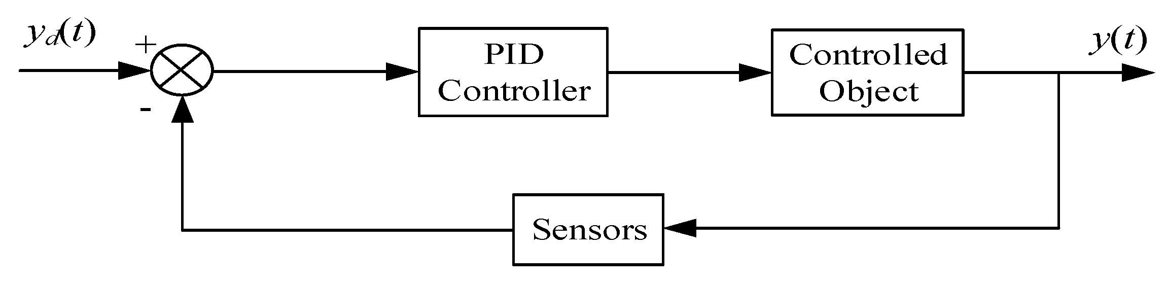
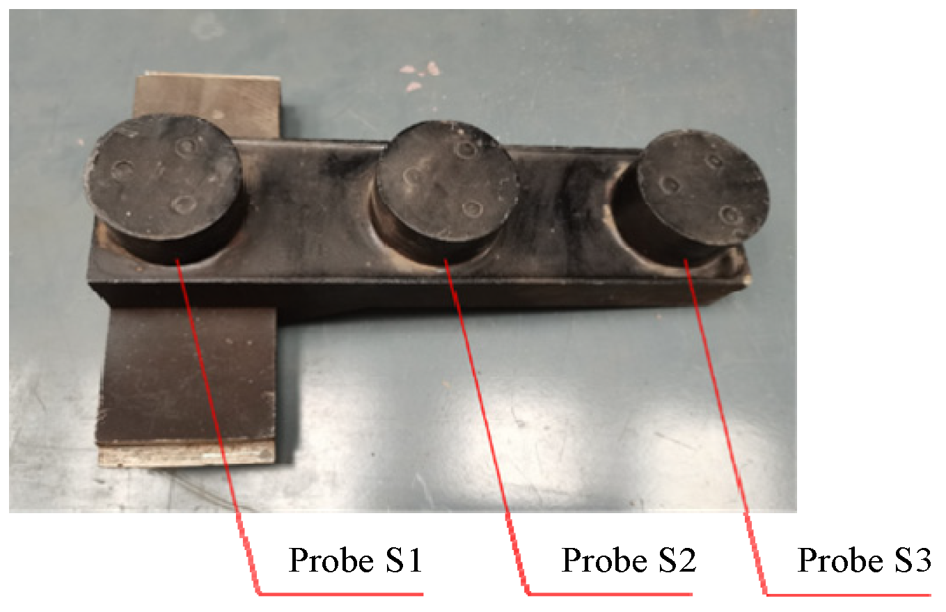
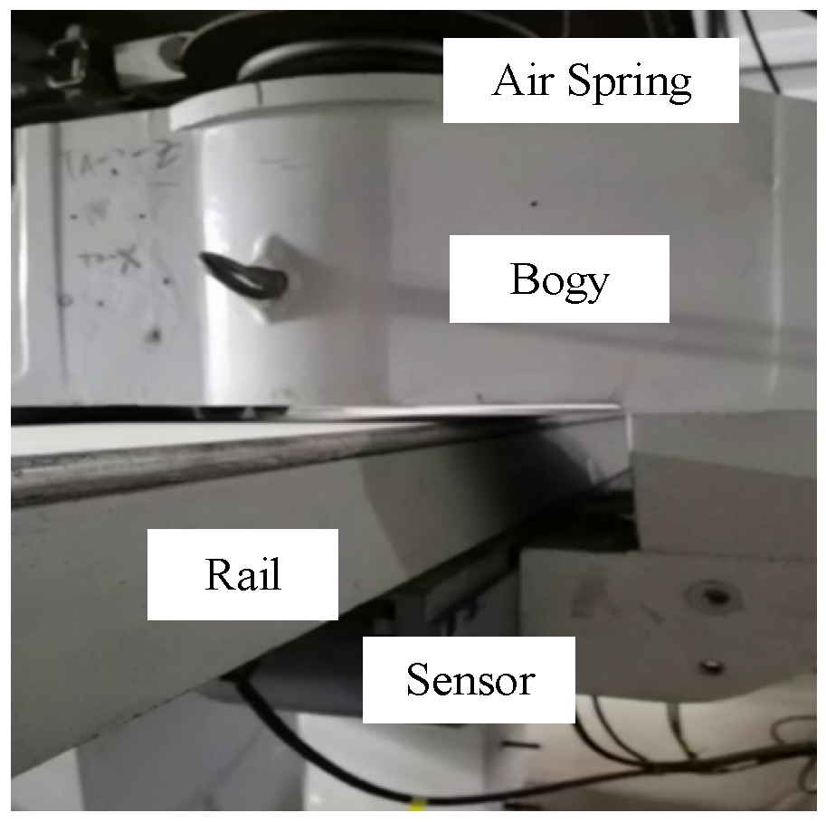
2.1. Control Strategy and Gap Sensor Design for Suspension System

The control strategy of the suspension system mainly adopts feedback control. In order to ensure the reliability of the suspension and the stationarity of the vehicle operation, the current in the electromagnet must be precisely controlled so that the suspension system has a good electromagnetic force to control the suspension gap. PID controller is used to control the suspension system by the air gap sensor which measures the gap, as shown in Figure 2.

The control deviation is formed according to the given value $y_d\left(t\right)$ and the actual output value $y\left(t\right)$.

$$error\left(t\right)=y_{\mathrm{d}}\left(t\right)-y\left(t\right)$$

(1)

The PID control rule is

$$u\left(t\right)=k_{\mathrm{p}}\left[error\left(t\right)+{\displaystyle \frac{1}{T_1}}{\displaystyle {\int }_0^{t}error\left(t\right)\mathrm{d}}t+{\displaystyle \frac{T_{\mathrm{D}}\mathrm{d}error\left(t\right)}{\mathrm{d}t}}\right]$$

(2)

The form of PID control transfer function is

$$G\left(s\right)={\displaystyle \frac{U\left(s\right)}{E\left(s\right)}}=k_{\mathrm{p}}\left(1+{\displaystyle \frac{1}{T_{1}s}}+T_{D}s\right)$$

(3)

where k_p is the proportional coefficient, T₁ is the integral time constant, and T_D is the differential time constant. The proportional link serves to represent the deviation signal error(t) of the control system in a proportional manner. The integrated sensor of the suspension system has the function of suspension gap detection and suspension acceleration detection at the same time. For suspension gap detection, the sensor has three probes, namely, probes S1, S2, and S3, as shown in Figure 3.

The three probes work independently and do not affect each other, the gap measurement range is 5–25 mm, the output is 0–20 mA, and the sensitivity is 1 mA/mm.

2.2. Clearance Variation Characteristics of Suspension System

In the magnetic suspension bogie with data collected in this experiment, an integrated sensor is installed at each end of each suspension module, which mainly monitors the distance between the suspension electromagnet and the track. The experimental platform is shown in Figure 4.

After multiple data acquisitions and comparative analyses, PID control parameters of the levitation controller are selected to make the fluctuation of floating as small as possible. On this basis, the suspension gap data are collected experimentally, and after the data is processed by Kalman filter, the suspension gap fluctuation characteristics of the single-section bogie of the maglev vehicle can be obtained, as shown in Figure 5.

From Figure 5, the suspension system has good suspension characteristics when floating statically. The frequency and amplitude of the fluctuation of the suspension gap are related to the PID parameters. Different controller parameters will affect the frequency and amplitude of the suspension gap. Due to the negative feedback control, the suspended electromagnet exhibits periodic vertical vibration characteristics. Since the electromagnet is rigidly connected to the bogie, the bogie of the suspended vehicle also demonstrates periodic vertical vibration characteristics, leading to both simple harmonic excitation and additional vibration characteristics in the bogie system. However, at present, there are still many unresolved issues regarding how precisely this vibration characteristic affects the dynamic performance of the suspended vehicles, as well as the vibration transmission laws under complex working conditions. A comprehensive investigation into these vibration characteristics is of critical importance for optimizing the dynamic performance of suspended vehicles, improving operational stability and ride comfort, and ensuring the safe and reliable operation of high-speed maglev transportation systems.

3. Dynamic Model and Steady-State Response Solution of Fractional-Order Vibration Isolation System

3.1. Equation of the Dynamics for the Vibration Isolation System

To study the dynamic performance of the secondary suspension, the core lies in its influence on the dynamic performance of the maglev vehicle system, so it is necessary to combine the equivalent mechanical model of the air spring with the dynamics of the vehicle system. Based on the aforementioned experimental data, external excitation factors such as aerodynamic forces and track irregularities are neglected. Given that the suspension system exhibits certain dynamic characteristics under foundation excitation, the fractional-order nonlinear Nishimura model is employed to describe the memory-restoring force characteristics of the air spring and the hyperelasticity of viscoelastic materials. The mechanical model of the suspension system is shown in Figure 6.

Figure 6 shows the mechanical model of the suspension system, where M is the mass of the suspension system; Y_B is periodic basic excitation; excitation amplitude is based on Y_S; X_A is the displacement of the vehicle body; X_B is the displacement of the nodes of the air spring mechanical model; $\Omega$ is the base excitation frequency; $K_1$ and $K_2$ are the stiffness coefficients of linear elastic restoring force; $C$ is the viscous damping coefficient; $F_K$ is the cubic nonlinear elastic restoring force, whose expression is $F_K=K_3\left(X_A-Y_B\right)+K_4{\left(X_A-Y_B\right)}^3$; $D$ is a fractional differential term; and $K$ is the coefficient of the fractional-order term. The dynamic differential equation of suspension system is as follows:

$$\left\{\begin{array}{c}M{\ddot{X}}_A+K_1\left(X_A-X_B\right)+K_3\left(X_A-Y_B\right)+K_4{\left(X_A-Y_B\right)}^3+K{D}_T^p[X_A\left(T\right)-Y_B\left(T\right)]=0\\ K_1\left(X_A-X_B\right)=K_2\left(X_B-Y_B\right)+C\left({\dot{X}}_B-{\dot{Y}}_B\right)\end{array}\right.$$

(4)

The system parameters are replaced by the following variables:

$$\left\{\begin{array}{l}{X}_1=X_A-Y_B\\ X_2=X_B-Y_B\end{array}\right.$$

(5)

The dynamic differential equation of the suspension system after parameter transformation is as follows:

$$\left\{\begin{array}{c}M{\ddot{X}}_1+K_1\left(X_1-X_2\right)+K_3{X}_1+K_4{X}_1^3+K{D}_T^P\left[X_1\left(T\right)\right]=-M{\ddot{Y}}_B\\ K_1\left(X_1-X_2\right)=C{\dot{X}}_2+K_2{X}_2\end{array}\right.$$

(6)

The reference parameter of the basic excitation amplitude $\overline{y}$ is introduced into Y_S, and the system parameters are replaced by the following variables:

$$\begin{array}{l}{\mathrm{\Omega }}_0=\sqrt{{\displaystyle \frac{K_1}{M}}},t={\mathrm{\Omega }}_{0}T,\omega ={\displaystyle \frac{\Omega }{{\mathrm{\Omega }}_0}},f_s={\displaystyle \frac{Y_K}{K_1}},X_i=f_s{x}_i,\overline{y}={\displaystyle \frac{Y_S}{f_s}}\\ {\mu }_{k2}={\displaystyle \frac{K_2}{K_1}},{\mu }_{k3}={\displaystyle \frac{K_3}{K_1}},\lambda ={\displaystyle \frac{K}{K_1}},\epsilon ={\displaystyle \frac{K_4}{K_1}}{f_s}^2,2\xi ={\displaystyle \frac{C}{\sqrt{K_{1}M}}}\end{array}$$

The dimensionless differential equation of the suspension system is as follows:

$$\left\{\begin{array}{c}{\ddot{x}}_1+(1+{\mu }_{k3})x_1-x_2+\epsilon {x_1}^3+\lambda D_t^p[x_1(t)]={\omega }^2\overline{y}\cos \left(\omega t\right)\\ x_1-x_2=2\xi {\dot{x}}_2+{\mu }_{k2}{x}_2\end{array}\right.$$

(7)

3.2. Fractional Calculus and Approximation Schemes

Let the first-order harmonic response of mass blocks and nodes be

$$x_1=A_1\cos \left(\omega t\right)+B_1\sin \left(\omega t\right)=A_{11}\sin \left(\omega t+{\theta }_1\right)$$

(8)

$$x_2=a_1\cos \left(\omega t\right)+b_1\sin \left(\omega t\right)=a_{11}\sin \left(\omega t+{\phi }_1\right)$$

(9)

The definition of Caputo is stated as follows:

$$D_t^p[x(t)]={\displaystyle \frac{1}{\mathrm{\Gamma }\left(1-p\right)}}{\displaystyle {\int }_0^t\frac{x^{\prime }(u)}{{(t-u)}^p}}\mathrm{d}u$$

(10)

$$\Gamma (y+1)=y\Gamma (y)$$

(11)

where $\Gamma \left(n\right)$ denotes the Gamma function that satisfies Equation (11).

When the fractional-order p is between 0 and 1, let $x\left(u\right)=A_{11}\sin (\omega t+{\theta }_1)$,

$$D_t^p\left[x_{11}\right(t\left)\right]={\displaystyle \frac{A_{11}\omega }{\Gamma (1-p)}}{\int }_0^t{\displaystyle \frac{\cos (\omega u+{\theta }_1)}{(t-u{)}^p}}\mathrm{d}u$$

(12)

Next, introduce $s=t-u$, then $\mathrm{d}s=-\mathrm{d}u$.

$$D_t^p[x_{11}(t)]={\displaystyle \frac{A_{11}\omega \cos (\omega t+{\theta }_1)}{\Gamma (1-p)}}{\displaystyle {\int }_0^t\frac{\cos (\omega s)}{s^p}}\mathrm{d}s+{\displaystyle \frac{A_{11}\omega \sin (\omega t+{\theta }_1)}{\Gamma (1-p)}}{\displaystyle {\int }_0^t\frac{\sin (\omega s)}{s^p}}\mathrm{d}s$$

(13)

Introduce the formula in Refs. [26,27]:

$${\displaystyle {\int }_0^t\frac{\cos (\omega s)}{s^p}}\mathrm{d}s={\omega }^{p-1}\left\{\Gamma (1-p)\sin \left({\displaystyle \frac{p\pi }{2}}\right)+{\displaystyle \frac{\sin (\omega t)}{{(\omega t)}^p}}+O\left[{(\omega t)}^{-p-1}\right]\right\}={\omega }^{p-1}\Gamma (1-p)\sin \left({\displaystyle \frac{p\pi }{2}}\right)$$

(14)

$${\displaystyle {\int }_0^t\frac{\sin (\omega s)}{s^p}}\mathrm{d}s={\omega }^{p-1}\left\{\Gamma (1-p)\cos \left({\displaystyle \frac{p\pi }{2}}\right)+{\displaystyle \frac{\cos (\omega t)}{{(\omega t)}^p}}+O\left[{(\omega t)}^{-p-1}\right]\right\}={\omega }^{p-1}\Gamma (1-p)\cos \left({\displaystyle \frac{p\pi }{2}}\right)$$

(15)

By substituting Equations (14) and (15) into Equation (13), the simplification can be obtained:

$$D_t^p[x_{11}(t)]=A_{11}\left[\omega \cos (\omega t+{\theta }_1){\omega }^{p-1}\sin \left({\displaystyle \frac{p\pi }{2}}\right)+\sin (\omega t+{\theta }_1){\omega }^p\cos \left({\displaystyle \frac{p\pi }{2}}\right)\right]$$

(16)

According to Equation (16), another expression of the fractional differential term defined by Caputo can be obtained.

$$D_t^p\left[x_{11}(t)\right]={\left(\omega \right)}^{p-1}\sin \left({\displaystyle \frac{p\pi }{2}}\right){\dot{x}}_{11}\left(t\right)+{\left(\omega \right)}^p\cos \left({\displaystyle \frac{p\pi }{2}}\right)x_{11}\left(t\right)$$

(17)

It can be seen that the fractional differential term is related to the displacement and velocity of the motion state of the system at the current time and changes with time in the numerical iteration process. In each iteration of the time step, the displacement and velocity are updated not only based on the external excitation at the current moment but also on the dynamics of the system itself, and the fractional-order operator changes as these quantities are updated. This is similar to the mechanism by which the original fractional-order operator affects the current state by continuously accumulating historical information through integration while dealing with continuous time. In the discrete numerical iterative environment, the accumulation of historical information is reflected through the updating of displacement and velocity and the corresponding changes of fractional-order operators. Therefore, the original memory effect of fractional-order operators is not lost.

Based on Equation (17), this approach successfully incorporates both the viscoelastic properties of materials and their behavior dependent on frequency. Shen et al. [26] showed that a first-order trigonometric function can adequately model fractional-order derivatives in various practical engineering scenarios. In these situations, it is reasonable to simplify the fractional-order derivative by omitting higher-order terms.

By substituting Equation (17) into Equation (7), the simplification can be obtained:

$$\left\{\begin{array}{c}{\ddot{x}}_1+(1+{\mu }_{k3})x_1-x_2+\epsilon {x_1}^3+\alpha {\dot{x}}_{11}\left(t\right)+\beta x_{11}\left(t\right)={\omega }^2\overline{y}\cos \left(\omega t\right)\\ x_1-x_2=2\xi {\dot{x}}_2+{\mu }_{k2}{x}_2\end{array}\right.$$

(18)

where $\alpha =\lambda {\omega }^{p-1}\sin \left({\displaystyle \frac{p\pi }{2}}\right)$ and $\beta =\lambda {\omega }^p\cos \left({\displaystyle \frac{p\pi }{2}}\right)$.

3.3. Solution of the Steady-State Response

Equations (8) and (9) are substituted into Equation (18) to carry out the first-order harmonic balance process, and after harmonic balance of sine and cosine terms, it can be obtained:

$$\left\{\begin{array}{l}{\psi }_1{a}_{11}^3+{\psi }_2{a}_{11}={\omega }^2\overline{y}\sin \left({\phi }_1\right)\\ {\psi }_3{a}_{11}^3+{\psi }_4{a}_{11}={\omega }^2\overline{y}\cos \left({\phi }_1\right)\end{array}\right.$$

(19)

where Formula (19) satisfies the following formula:

$$\left\{\begin{array}{l}{\psi }_1=\left(3{\xi }^2\epsilon {\mu }_{k2}+3{\xi }^2\epsilon \right){\omega }^2+{\displaystyle \frac{3{\mu }_{k2}^3\epsilon }{4}}+{\displaystyle \frac{9{\mu }_{k2}^2\epsilon }{4}}+{\displaystyle \frac{9{\mu }_{k2}\epsilon }{4}}+{\displaystyle \frac{3\epsilon }{4}}\\ {\psi }_2=\left(-2\alpha \xi -{\mu }_{k2}-1\right){\omega }^2+\beta {\mu }_{k2}+{\mu }_{k2}{\mu }_{k3}+{\mu }_{k2}+{\mu }_{k3}+\beta \\ {\psi }_3=6{\xi }^3\epsilon {\omega }^3+\left({\displaystyle \frac{3}{2}}{\mu }_{k2}^2\xi \epsilon +3{\mu }_{k2}\xi \epsilon +{\displaystyle \frac{3}{2}}\epsilon \xi \right)\omega \\ {\psi }_4=-2\xi {\omega }^3+\left(\alpha {\mu }_{k2}+2\xi \beta +2\xi {\mu }_{k3}+\alpha +2\xi \right)\omega \end{array}\right.$$

(20)

The steady-state response solution of node amplitude and phase can be obtained:

$${\left({\omega }^2\overline{y}\right)}^2={\left({\psi }_1{a}_{11}^3+{\psi }_2{a}_{11}\right)}^2+{\left({\psi }_3{a}_{11}^3+{\psi }_4{a}_{11}\right)}^2$$

(21)

$${\phi }_1=\arctan \left({\displaystyle \frac{{\psi }_1{a}_{11}^3+{\psi }_2{a}_{11}}{{\psi }_3{a}_{11}^3+{\psi }_4{a}_{11}}}\right)$$

(22)

Through the collected suspension data of the maglev vehicle it can be seen that although there is a small fluctuation in the suspension process, the amplitude of the fluctuation is very small, which is because the more appropriate control parameters are selected. If the control parameters are changed, the suspension fluctuation will also change, and the improper selection of control parameters will even increase the suspension gap. This section simulates the dynamic performance of the suspension system through numerical simulation. Equation (18) is the non-dimensional differential equation of motion of the system, and its state parameters can be obtained by transforming as follows:

$$\left\{\begin{array}{c}{y}_1=x_1\\ y_2={\dot{x}}_1\\ y_3=x_2\end{array}\right.$$

(23)

By substituting Equation (23) into Equation (18) and then reducing the order of the differential equation of the motion of the system, the equation of the motion state of the system can be obtained as follows:

$$\left\{\begin{array}{l}{\dot{y}}_1=y_2\\ {\dot{y}}_2={\omega }^2\overline{y}\cos \left(\omega t\right)-\left(1+{\mu }_{k3}\right)y_1+y_3-\epsilon {y_1}^3-\lambda D_t^p\left[y_1\left(t\right)\right]\\ {\dot{y}}_3={\displaystyle \frac{y_1-\left(1+{\mu }_{k2}\right)y_3}{2\xi }}\end{array}\right.$$

(24)

where $y_1,y_2,y_3$ represents displacement of mass block, velocity of mass block, and displacement of node of vibration isolation system, respectively.

3.4. Motion State and Stability Identification

To gain a comprehensive understanding of periodic motions, it is essential to delve into specific characteristics in detail. When examining the variations and local fluctuations of periodic motions in the low-frequency domain, this study introduces a technique referred to as the Poincaré mapping. This method helps analyze the behavior of these motions by capturing their evolution at discrete intervals. The Poincaré mapping section ${\sigma }_{\tau }=\{(x,\dot{x})\in R^2\times S,\theta \mathrm{mod}2\pi =0\}$ serves to identify if periodic motions exist within the system. Employing the Lyapunov exponential spectrum serves as an effective method for determining if the dynamic system exhibits periodic or chaotic characteristics [28,29]. By applying Poincaré mapping, a continuous dynamic system is transformed into a discrete dynamic system, while an appropriate computational approach is also presented.

$${\lambda }_i={\displaystyle \frac{1}{K}}{\displaystyle \sum _{k=1}^K\ln ‖z_i^{\left(k\right)}‖}$$

(25)

where K denotes the number of iterations, $z_i^{\left(k\right)}$ represents the vector, which has been subjected to Gram–Schmidt orthogonalization and norm normalization after every iteration, and $‖z_i^{\left(k\right)}‖\left(i=1,2,3\right)$ is the norm of $z_i^{\left(k\right)}$. The Lyapunov exponent acts as a key instrument for evaluating if the system exhibits stable periodic patterns or chaotic properties. It is essential in distinguishing between these two unique dynamic conditions, thereby facilitating a deeper insight into the stability attributes of the system.

Furthermore, the cell mapping method functions as a reliable tool for analyzing nonlinear dynamical systems. This approach divides the state space of the system into multiple distinct areas. By studying the transitions of the system’s state between these areas, the dynamic properties of the system can be precisely described. This method improves our understanding of state transitions in complex nonlinear systems, offering more profound insights into the evolution from one state to another [30,31,32]. In this research, we utilize the cell mapping method to distinguish between stable and unstable solutions by analyzing the frequency of transitions between cells and the distribution patterns within individual cells.

4. Results and Discussion

4.1. The Characteristics of the Amplitude of Main Resonance Excitation and Response

Based on the suspension data collected by the experiment, the influence of the frequency of the suspension wave and the change of the amplitude of the suspension wave on the dynamic behavior of the suspension system is considered. Select the following dimensionless parameters: $\lambda =0.01$, $\epsilon =0.6$, $\omega =0.5$, $\xi =0.05$, $p=0.5$, ${\mu }_{k2}=0.01$, ${\mu }_{k3}=0.01$.

To verify the accuracy of the harmonic balance method (HB) in solving the problem, the steady-state solution of the dynamic response was solved by combining the fourth-order Runge–Kutta numerical integration algorithm (RK4). The results show that the analytical approximate solution obtained is close to the numerical solution, as shown in Figure 7.

As shown in Figure 7, it is evident that there is a strong correlation between the numerical results obtained from the approximated equations and those from the exact equations. The multi-amplitude characteristics of the system at low frequency are shown in Figure 8.

As can be seen from Figure 8a, when the external excitation frequency remains unchanged while the amplitude $\overline{y}$ changes, the multi-valued amplitude curve of the system will show the coexistence of polymorphic solutions with the increase in the excitation amplitude $\overline{y}$, the multi-valued amplitude curve will show the jump phenomenon, and the excitation amplitude $\overline{y}$ corresponding to the jump phenomenon is consistent with the excitation amplitude $\overline{y}$ of the saddle-node bifurcation (SNB) mutation in the bifurcation diagram. The amplitude curve jumps upward, and the bifurcation diagram also changes upward.

As can be seen from Figure 8b, the multi-valued amplitude curve of the system shows a downward jump phenomenon with the decrease in the excitation amplitude $\overline{y}$, and the excitation amplitude $\overline{y}$ corresponding to the downward jump phenomenon is consistent with the excitation amplitude $\overline{y}$ of the downward abrupt change of the saddle-node bifurcation (SNB) in the bifurcation diagram.

As shown in Figure 8c, as $\epsilon$ increases, the amplitude corresponding to the SNB bifurcation jump point of the amplitude curve gradually decreases, and the corresponding excitation amplitude $\overline{y}$ also gradually decreases. When the excitation amplitude exceeds the coexistence range of multiple solutions at the same excitation amplitude $\overline{y}$, the amplitude of the amplitude curve corresponding to the larger $\epsilon$ is smaller, indicating that the larger $\epsilon$ significantly suppresses the amplitude of the response.

As shown in Figure 8d, with the increase in $\lambda$, the range where multiple steady-state solutions coexist in the amplitude curve gradually decreases. Under the same excitation amplitude $\overline{y}$, the amplitude curve corresponding to the larger $\lambda$ on the left side of the coexistence of multiple solutions is greater, while the amplitude of the amplitude curve corresponding to the larger $\lambda$ on the right side of the coexistence of multiple solutions is smaller.

As shown in Figure 8e, with the increase in $p$, the amplitude corresponding to the SNB bifurcation jump point of the amplitude curve gradually increases, and the range of coexistence of multiple stable states gradually shifts to the right. Under the same excitation amplitude $\overline{y}$, the amplitude of the amplitude curve corresponding to the larger $p$ on the left side of the coexistence of multiple states is smaller, while the amplitude of the amplitude curve corresponding to the larger $p$ on the right side of the coexistence of multiple states is larger.

As shown in Figure 8f, with the increase in ${\mu }_{k2}$, the amplitude corresponding to the SNB bifurcation jump point of the amplitude curve gradually decreases, and the range of the excitation amplitude $\overline{y}$ where multiple steady-state solutions coexist gradually decreases and shifts to the left. Under the same excitation amplitude $\overline{y}$, the amplitude of the amplitude curve corresponding to the larger ${\mu }_{k2}$ on the left side of the coexistence of multiple solutions is larger, while the amplitude of the amplitude curve corresponding to the larger ${\mu }_{k2}$ on the right side of the coexistence of multiple solutions is smaller.

As illustrated in Figure 8g, as ${\mu }_{k3}$ increases, the amplitude at the SNB bifurcation jump point of the amplitude curve progressively diminishes, and the range of excitation amplitude $\overline{y}$ for which multiple steady-state solutions coexist gradually narrows and shifts to the left. For a given excitation amplitude $\overline{y}$, the amplitude curve exhibits a higher amplitude on the left side of the coexistence region when ${\mu }_{k3}$ is larger, while it shows a lower amplitude on the right side of the coexistence region for larger ${\mu }_{k3}$.

As shown in Figure 8h, with the increase in $\omega$, the amplitude corresponding to the SNB bifurcation jump point of the amplitude curve increases, and the range of the excitation amplitude $\overline{y}$ where multiple steady-state solutions coexist gradually expands and shifts to the right. Under the same excitation amplitude $\overline{y}$, the amplitude of the amplitude curve corresponding to the larger $\omega$ on the left side of the coexistence of multiple solutions is smaller, while the amplitude of the amplitude curve corresponding to the larger $\omega$ on the right side of the coexistence of multiple solutions is larger.

As shown in Figure 8i, with the increase in $\xi$, the corresponding $\overline{y}$ at the SNB bifurcation jump point of the amplitude curve increases, and the coexistence range of multi-stable solutions decreases and shifts to the right. Under the same excitation amplitude $\overline{y}$, the amplitude of the amplitude curve corresponding to the larger $\xi$ on the left side of the coexistence of multi-stable solutions is larger, while the amplitude of the amplitude curve corresponding to the larger $\xi$ on the right side of the coexistence of multi-stable solutions is smaller.

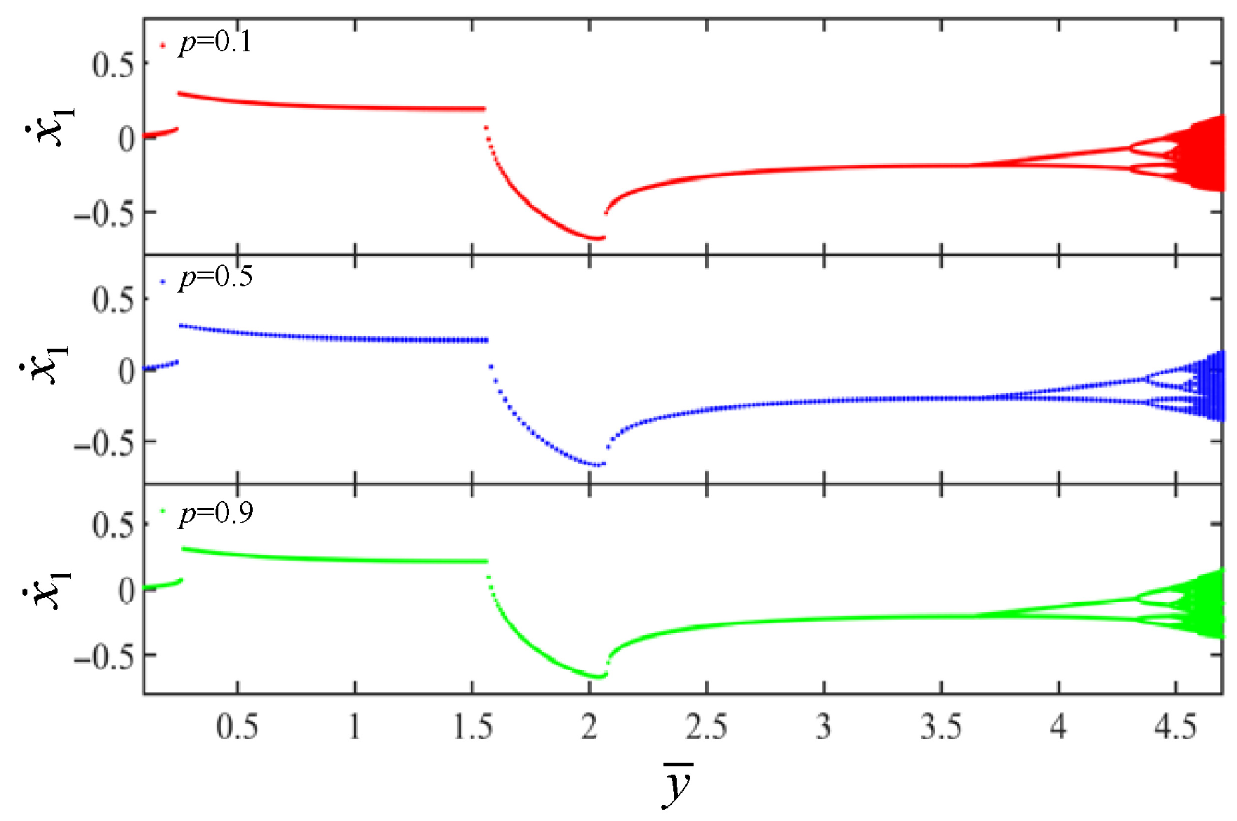
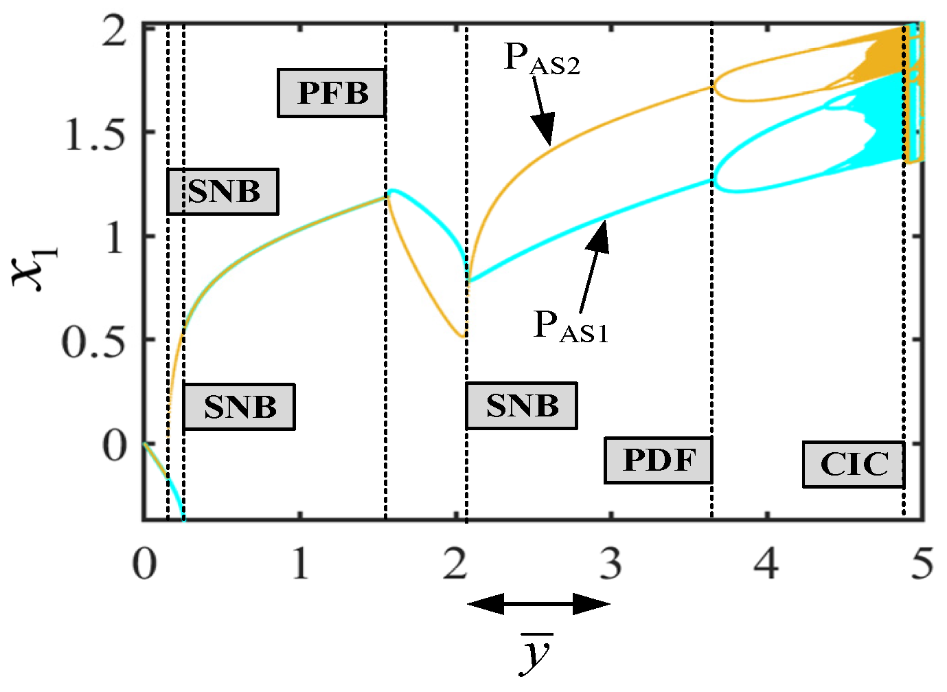
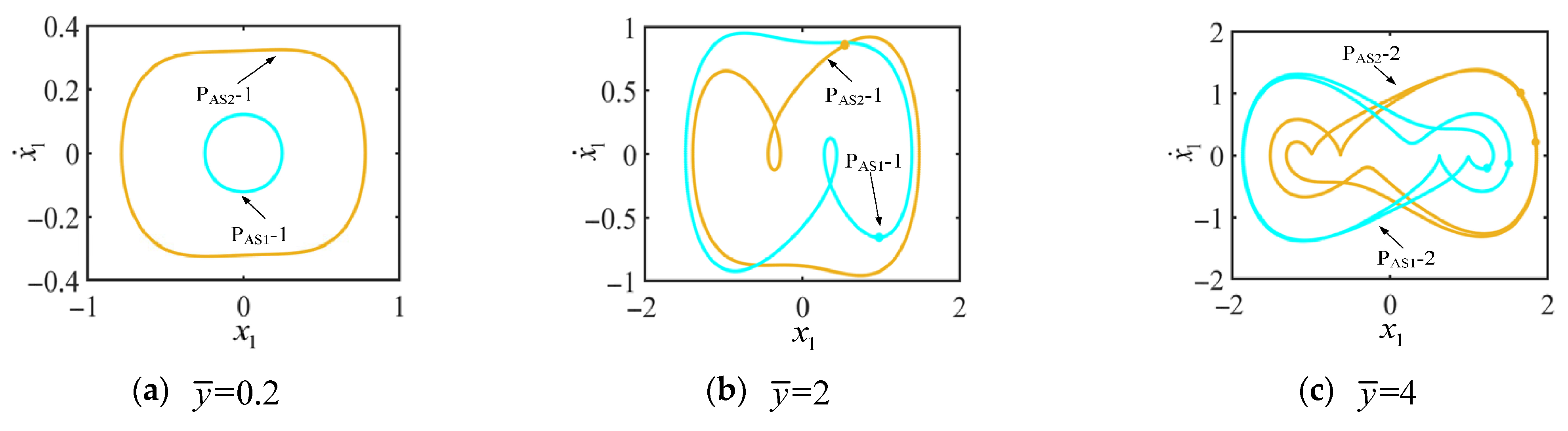
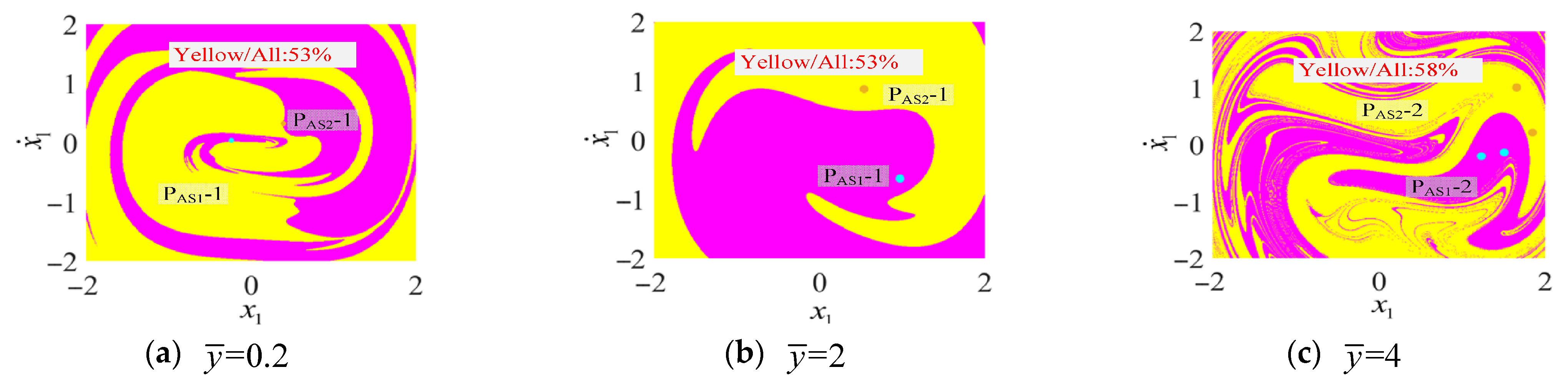
4.2. The Impact of Suspension Gap Amplitude on the Diversity of Periodic Motion Characteristics

Due to the presence of fractional-order differential terms in the model, the influence laws of different fractional-order exponents p on the dynamical transition process of the system are analyzed below.

The system parameter are selected as $\lambda =0.01$, $\epsilon =0.6$, $\omega =0.5$, $\xi =0.05$, ${\mu }_{k2}=0.01$, and ${\mu }_{k3}=0.01$. The values of parameter p are selected as 0.1, 0.5, and 0.9. The influences of different fractional-order p values on the dynamic response are shown in Figure 9.

As shown in Figure 9, with the increase in the basic excitation $\overline{y}$, the system undergoes a series of bifurcations from the periodic motion with period 1 and eventually enters chaos. Different fractional-order p values do not change the essential laws of the transition process of the periodic motion. To take into account the viscoelasticity of the model simultaneously, the fractional-order p is selected as 0.5 below. The bifurcation and motion transition rule of the system in the low-frequency region were shown in Figure 9.

As can be seen from Figure 10, with the change of excitation amplitude, there are various bifurcation types in the system, including period-doubled bifurcation (PDB), inverse period-doubled bifurcation (IPDB), pitchfork bifurcation (PFB), inverse pitchfork bifurcation (IPFB), saddle-node bifurcation (SNB), Catastrophic Bifurcation (CIC), and Boundary Crisis (BC).

In the transition process of the system from periodic motion to chaos induced by the above types of bifurcation, SNB occurs many times. The two SNBs in the low-amplitude region are consistent with the jump amplitude of the multi-value amplitude curve. The first SNB is consistent with the downward jump amplitude of the multi-value amplitude curve, and the second SNB is consistent with the upward jump amplitude of the multi-valued amplitude curve.

Different from the first two SNBs, the system generates a pair of anti-symmetric moving tracks P_AS1 and P_AS2 under the induction of the PFB. The third SNB makes the relative positions of the displacements of Poincaré attractors on the anti-symmetric moving tracks swap. The system jumps up and down at the same amplitude at the same time. The trajectory of moving phase under different excitation amplitudes is shown in Figure 11.

As can be seen from Figure 11, the system has different dynamic behaviors in the amplitude range of multi-stable coexistence. When the system excitation amplitude $\overline{y}$ is 0.2, two moving tracks P_AS1 and P_AS2 appear in the system, in which the track P_AS1 has the dynamic behavior of the upper branch of the multi-amplitude curve and the track P_AS2 has the dynamic behavior of the lower branch of the multi-amplitude curve, as shown in Figure 11a. Under the induction of the PFB, a pair of anti-symmetric motions appear in the system, as shown in Figure 11b. With the change in the excitation amplitude $\overline{y}$, under the induction of PDB, two anti-symmetric moving tracks enter period-two motion, as shown in Figure 11c.

In order to further study the distribution of different attractors and their attractor domains in the region of polymorphic coexistence, the initial state domain ${\Omega }_a=\left\{\left.\left(x_1,{\dot{x}}_1\right)\right|-3<x_1<3,-5<{\dot{x}}_1<5\right\}$ was selected and divided into $1000\times 1000$ state cells. The motion states and attractor domains of the system under different excitation amplitudes $\overline{y}$ were shown in Figure 12.

As can be seen from Figure 12a, when the fundamental excitation amplitude $\overline{y}$ is 0.2, the system is in the range of coexistence of polymorphic solutions, and there are two attractive domains in the system, among which the ratio of P_AS1-1 attractive domain to the full initial state domain is 53%. It can be seen from Figure 12b that when the excitation amplitude $\overline{y}=2$, a pair of anti-symmetric motions will appear in the system induced by the PFB, accompanied by two attractive domains, of which the ratio of P_AS2-1 attractive domain to the total initial state domain is 53%. It can be seen from Figure 12c that when the excitation amplitude $\overline{y}=4$, the system is between periodic motion and chaos, and the two pairs of anti-symmetric motions are in periodic binary motion at the same time, in which the ratio of the P_AS2-2 attractive domain to the full initial state domain is 58%. It can be seen that under the induction of the PFB, the attraction domain of the anti-symmetric motion trajectory also changes. Although both of them are in T-1 motion, the ratio of the attraction domain of the anti-symmetric motion to the total initial state domain on both sides of the PFB changes.

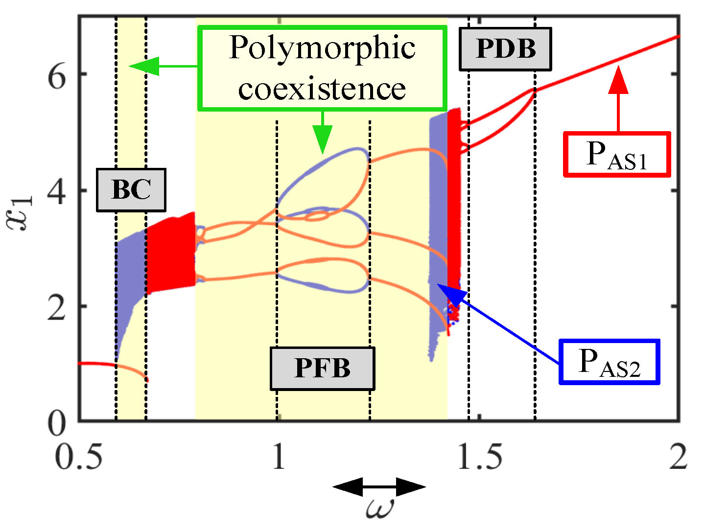
4.3. The Impact of Varying Frequencies on the Diversity of Periodic Motion Characteristics

The subsequent analysis examines the impact of varying excitation frequencies on the diversity of periodic motion and the associated transition mechanisms. The system parameters are selected as $\lambda =0.01$, $\epsilon =0.6$, $\overline{y}=10$, $\xi =0.05$, $p=0.5$, ${\mu }_{k2}=0.01$, and ${\mu }_{k3}=0.01$. When subjected to harmonic excitation, the system sequentially demonstrates a range of bifurcation types, including PFB, PDB, and BC throughout the evolution of periodic motion. The reverse phenomena of certain bifurcations are referred to as inverse IPFB and IPDB. Furthermore, during the multi-initial-value forward and backward frequency scanning process, the system exhibits the coexistence of multiple states, as illustrated in Figure 13.

As the excitation frequency rises, the system initially exhibits P_AS1-1 motion. Following BC influence, it shifts from P_AS1-1 to a state of P_AS1-chaos. With further increases in ω, intermittent phase doubling bifurcations drive the system into P_AS1-3 motion. The coexistence of multiple states ceases under IPFB, transitioning the system from P_AS1-3 to T-3 motion. As ω continues to rise, PFB induces a reversal, shifting the system back from T-3 to P_AS1-3. motion. Subsequently, PDB prompts the system to evolve from P_AS1-3 to P_AS1-6 motion. Under IPDB influence, the system reverts from P_AS1-6 to P_AS1-3 motion. BC then triggers another shift, driving the system from P_AS1-3 into P_AS1-chaos. A series of IPDBs subsequently guide the system through T-2 motion, eventually stabilizing at T-1 motion. In terms of dynamical characteristics, during periodic motions, the maximum Lyapunov exponent remains below 0. In contrast, when the system transitions into P_AS1-chaos, this exponent exceeds 0. At bifurcation points induced by various mechanisms, the maximum Lyapunov exponent approaches or equals 0. Detailed insights into these transitions and their associated Lyapunov exponent are shown in Figure 14a.

As the excitation frequency reduces, the system initially exhibits T-1 motion. Following a sequence of PDB influences, it evolves into a P_AS2-chaos motion state, characterized by the maximum Lyapunov exponent exceeding 0. Under BC influence, the system transfers to the T-3 motion state, where the maximum Lyapunov exponent is below 0. With further reduction in $\omega$ and under PFB influence, the system transitions to the P_AS2-3 motion state. Subsequently, driven by PDB effects, it moves into the P_AS2-6 motion state. As $\omega$ continues to decline, IPDB influence induces the system to re-enter the P_AS2-3 motion state. After that, under IPFB influence, the system transitions back to the T-3 motion state, maintaining a maximum Lyapunov exponent less than 0. Further decrease in w, combined with PFB influence, causes the T-3 motion state to transition to the P_AS2-3 motion state. A subsequent series of PDB influences then drives the system into the P_AS2-chaos motion state, marked by a maximum Lyapunov exponent greater than 0. Finally, under BC influence, the system returns to the T-1 motion state, with the maximum Lyapunov exponent remaining below 0. The detailed transition process and corresponding maximum Lyapunov exponents are illustrated in Figure 14b.

In the process of forward and reverse frequency sweeping, the system demonstrates the coexistence of multiple solutions due to the influence of PFB, with the phase trajectory exhibiting a pair of antisymmetric motions. At $\omega =0.6$, the system displays a coexistence of P_AS1-1 motion and P_AS2-chaos. At $\omega =0.8$, it shows a coexistence of P_AS1-3 motion and P_AS2-3. At $\omega =1$, the system continues to exhibit a coexistence of P_AS1-3 motion and P_AS2-3. At $\omega =1.1$, it presents a coexistence of P_AS1-6 motion and P_AS2-6. At $\omega =1.18$, the system once again exhibits a coexistence of P_AS1-3 motion and P_AS2-3. At $\omega =1.4$, the system still shows a coexistence of P_AS1-3 motion and P_AS2-chaos. The maximum Lyapunov exponent associated with P_AS1-3 motion is less than 0, whereas that linked to P_AS2-chaos is greater than 0. The variety of periodic motions, the transition processes between periodic motions and chaos within the system, as well as the distribution of attractors in the phase trajectory and Poincaré section, are illustrated in Figure 15.

5. Conclusions

In this paper, the equivalent mechanical model of the suspension system is established considering the super-elasticity and memory-restoring force characteristics of the secondary suspension air spring, and the dynamic differential equation of the suspension system under the foundation excitation is obtained. The first-order harmonic balance method is used to obtain the variation law of the amplitude of suspension system and the amplitude of foundation excitation, and the variation law of the jump phenomenon and the diversity of periodic motion of the multi-value amplitude curve are summarized. The numerical simulation also found that when the gap of the suspension system changed, the coexistence of multi-periodic motion existed in the system. Combined with the cell mapping algorithm, the distribution law of different attractors on the attraction domain of periodic motion was discussed, and the rule of the transition of periodic motion with different fundamental excitation amplitude was summarized. The dynamic stability of the suspension system was analyzed with the Lyapunov exponent, and the following conclusions were obtained:

(1) When the frequency of the base excitation is fixed but the amplitude of the base excitation changes, the multi-valued amplitude curve of the system has the phenomenon of multi-state solution coexistence. When the amplitude of the foundation excitation is small, the system will also have a jump phenomenon, and the direction of the jump phenomenon is different with the change of the foundation excitation amplitude. The jump direction of the SNB is consistent with the jump direction of the multi-value amplitude curve.

(2) The coexistence of multi-valued amplitude solutions exists in the system when the fundamental excitation amplitude is small. With the increase in the fundamental excitation amplitude, the coexistence of multi-valued amplitude solutions no longer occurs in the multi-valued amplitude curve, but the periodic motion of the system is diverse. Under the induction of PFB, the system has two motion trajectories and presents antisymmetric phase trajectories. When the system enters chaos, the chaotic attractors combine with each other under the induction of CIC, and the phase trajectory changes from anti-symmetric motion to symmetric motion.

(3) In the process of the system transitioning from periodic motion to chaos, there are various types of bifurcation forms, and a pair of anti-symmetric motions are generated under the induction of fork bifurcation. In the multi-valued bifurcation diagram, the displacement of Poincaré attractors on the P_AS1 moving track is above the displacement of Poincaré attractors on the P_AS2 moving track. However, under the induction of the SNB, the relative position of the Poincaré attractors’ displacement changes, and the displacement of the Poincaré attractors’ displacement of the P_AS1 moving orbit is under the displacement of the Poincaré attractors’ displacement of the P_AS2 moving orbit.

(4) The variations in parameters significantly modify the curves that represent the relationships between excitation amplitude and response amplitude. This highlights the critical roles of each parameter in determining the amplitude characteristics of the system, providing essential insights into its underlying dynamic behaviors.

The dynamic behavior of the suspension system can be predicted under different gaps according to the changing laws of the dynamic behavior, which can avoid the dynamic performance instability of the system dynamic response in different excitation amplitude ranges. The research content of this paper not only provides a theoretical reference for predicting the dynamic performance of maglev systems under different clearance conditions but also, specifically tailored to the context of maglev vehicle air springs, offers a dynamic model that can serve as a theoretical basis for all damping systems exhibiting strong nonlinearity and frequency dependence.

References

1. Li, Q.; Li, S.; Li, F.; Xu, D.; He, Z. Analysis and Experiment of Vibration Isolation Performance of a Magnetic Levitation Vibration Isolator with Rectangular Permanent Magnets. J. Vib. Eng. Technol. 2020, 8, 751–760. [Google Scholar] [CrossRef]
2. Chen, X.; Sun, J.; Li, M.; Jiao, W.; Jiang, Y.; Hu, J. Compact Multiphysics Coupling Modeling and Analysis of Self-Excited Vibration in Maglev Trains. Appl. Math. Model. 2025, 141, 115915. [Google Scholar] [CrossRef]
3. Wang, S.M.; Ni, Y.Q.; Sun, Y.G.; Lu, Y.; Duan, Y.F. Modelling Dynamic Interaction of Maglev Train–Controller–Rail–Bridge System by Vector Mechanics. J. Sound Vib. 2022, 533, 117023. [Google Scholar] [CrossRef]
4. Tian, X.; Xiang, H.; Li, Y. Modeling and Analyzing of High-Speed Maglev Train-Bridge Systems Considering Centrifugal Force Induced by Bridge Vertical Deformation. Structures 2025, 73, 108240. [Google Scholar] [CrossRef]
5. Liang, S.; Zhai, M.; Long, Z. Parameter Impact Analysis and Vibration Control for High Speed Maglev Train-Track Coupling System with Experimental Verification. IEEE Trans. Veh. Technol 2025, 1–16. [Google Scholar] [CrossRef]
6. Yu, Y.; Zhou, W.; Zhang, Z.; Bi, Q. Analysis on the Motion of Nonlinear Vibration with Fractional Order and Time Variable Mass. Appl. Math. Lett. 2022, 124, 107621. [Google Scholar] [CrossRef]
7. Wang, J.; Zhang, R.; Liu, J. Vibrational Resonance Analysis in a Fractional Order Toda Oscillator Model with Asymmetric Potential. Int. J. Non-Linear Mech. 2023, 148, 104258. [Google Scholar] [CrossRef]
8. Zhao, K.; Ning, L. Vibrational Resonance in a Fractional Order System with Asymmetric Bistable Potential and Time Delay Feedback. Chin. J. Phys. 2022, 77, 1796–1809. [Google Scholar] [CrossRef]
9. Li, H.; Li, J.; Hong, G.; Dong, J.; Ning, Y. Fractional-Order Model and Experimental Verification of Granules-Beam Coupled Vibration. Mech. Syst. Signal Process. 2023, 200, 110536. [Google Scholar] [CrossRef]
10. Chen, Y.; Tai, Y.; Xu, J.; Xu, X.; Chen, N. Vibration Analysis of a 1-DOF System Coupled with a Nonlinear Energy Sink with a Fractional Order Inerter. Sensors 2022, 22, 6408. [Google Scholar] [CrossRef]
11. Wang, M.; Zhao, J.; Wang, R.; Qin, C.; Liu, P. Dynamical Characterisation of Fractional-Order Duffing-Holmes Systems Containing Nonlinear Damping Under Constant Simple Harmonic Excitation. Chaos Solitons Fractals 2025, 190, 115745. [Google Scholar] [CrossRef]
12. Ren, Y.; Li, L.; Wang, W.; Wang, L.; Pang, W. Magnetically Suspended Control Sensitive Gyroscope Rotor High-Precision Deflection Decoupling Method Using Quantum Neural Network and Fractional-Order Terminal Sliding Mode Control. Fractal Fract. 2024, 8, 120. [Google Scholar] [CrossRef]
13. Ivanov, D. Identification of Fractional Models of an Induction Motor with Errors in Variables. Fractal Fract. 2023, 7, 485. [Google Scholar] [CrossRef]
14. Han, Y.X.; Zhang, J.X.; Wang, Y.L. Dynamic Behavior of a Two-Mass Nonlinear Fractional-Order Vibration System. Front. Phys. 2024, 12, 1452138. [Google Scholar] [CrossRef]
15. Zhao, H.; Wang, F.; Zhang, Y.; Zheng, Z.; Ma, J.; Fu, C. Fractional-Order Modeling and Stochastic Dynamics Analysis of a Nonlinear Rubbing Overhung Rotor System. Fractal Fract. 2024, 8, 643. [Google Scholar] [CrossRef]
16. Cao, J.; Ma, C.; Jiang, Z.; Liu, S. Nonlinear Dynamic Analysis of Fractional Order Rub-Impact Rotor System. Commun. Nonlinear Sci. Numer. Simul. 2011, 16, 1443–1463. [Google Scholar] [CrossRef]
17. Hou, J.; Niu, J.; Shen, Y.; Yang, S.; Zhang, W. Dynamic Analysis and Vibration Control of Two-Degree-of-Freedom Boring Bar with Fractional-Order Model of Magnetorheological Fluid. J. Vib. Control 2022, 28, 3001–3018. [Google Scholar] [CrossRef]
18. Boulaaras, S.; Sriramulu, S.; Arunachalam, S.; Allahem, A.; Alharbi, A.; Radwan, T. Chaos and Stability Analysis of the Nonlinear Fractional-Order Autonomous System. Alex. Eng. J. 2025, 118, 278–291. [Google Scholar] [CrossRef]
19. Niu, J.; Wang, L.; Shen, Y.; Zhang, W. Vibration Control of Primary and Subharmonic Simultaneous Resonance of Nonlinear System with Fractional-Order Bingham Model. Int. J. Non-Linear Mech. 2022, 141, 103947. [Google Scholar] [CrossRef]
20. Yang, F.; Wang, P.; Wei, K.; Wang, F. Investigation on Nonlinear and Fractional Derivative Zener Model of Coupled Vehicle-Track System. Veh. Syst. Dyn. 2020, 58, 864–889. [Google Scholar] [CrossRef]
21. Chang, Y.; Zhu, Y.; Li, Y.; Wang, M. Dynamical Analysis of a Fractional-Order Nonlinear Two-Degree-of-Freedom Vehicle System by Incremental Harmonic Balance Method. J. Low Freq. Noise Vib. Act. Control. 2024, 43, 706–728. [Google Scholar] [CrossRef]
22. Dai, J.; Lim, J.G.Y.; Ang, K.K. Dynamic Response Analysis of High-Speed Maglev-Guideway System. J. Vib. Eng. Technol. 2023, 11, 2647–2658. [Google Scholar] [CrossRef]
23. Sun, Y.; He, Z.; Xu, J.; Sun, W.; Lin, G. Dynamic Analysis and Vibration Control for a Maglev Vehicle-Guideway Coupling System with Experimental Verification. Mech. Syst. Signal Process. 2023, 188, 109954. [Google Scholar] [CrossRef]
24. Wang, S.; Zhang, Y.; Guo, W.; Pi, T.; Li, X. Vibration Analysis of Nonlinear Damping Systems by the Discrete Incremental Harmonic Balance Method. Nonlinear Dyn. 2023, 111, 2009–2028. [Google Scholar] [CrossRef]
25. Qu, M.; Yang, Q.; Wu, S.; Ding, W.; Li, J.; Li, G. Analysis of Super-Harmonic Resonance and Periodic Motion Transition of Fractional Nonlinear Vibration Isolation System. J. Low Freq. Noise Vib. Act. Control. 2023, 42, 771–788. [Google Scholar] [CrossRef]
26. Shen, Y.J.; Wen, S.F.; Li, X.H.; Yang, S.P.; Xing, H.J. Dynamical Analysis of Fractional-Order Nonlinear Oscillator by Incremental Harmonic Balance Method. Nonlinear Dyn. 2016, 85, 1457–1467. [Google Scholar] [CrossRef]
27. Kong, F.; Han, R.; Zhang, Y. Approximate Stochastic Response of Hysteretic System with Fractional Element and Subjected to Combined Stochastic and Periodic Excitation. Nonlinear Dyn. 2022, 107, 375–390. [Google Scholar] [CrossRef]
28. Li, G.; Sun, J.; Ding, W. Dynamics of a Vibro-Impact System by the Global Analysis Method in Parameter-State Space. Nonlinear Dyn. 2019, 97, 541–557. [Google Scholar] [CrossRef]
29. Qu, M.; Wang, L.; Jin, Q.; Zhou, D.; Li, J. Nonlinear Dynamics of Nishimura Model-Based Fractional-Order Vibration Isolation System Under the Synergistic Effect of Aerodynamic Lift and Harmonic Excitation. Nonlinear Dyn. 2025, 113, 12693–12717. [Google Scholar] [CrossRef]
30. Gyebrószki, G.; Csernák, G. Clustered Simple Cell Mapping: An Extension to the Simple Cell Mapping Method. Commun. Nonlinear Sci. Numer. Simul. 2017, 42, 607–622. [Google Scholar] [CrossRef]
31. Zhang, Z.; Dai, L. The Application of the Cell Mapping Method in the Characteristic Diagnosis of Nonlinear Dynamical Systems. Nonlinear Dyn. 2023, 111, 18095–18112. [Google Scholar] [CrossRef]
32. Chandrashekar, A.; Belardinelli, P.; Staufer, U.; Alijani, F. Robustness of Attractors in Tapping Mode Atomic Force Microscopy. Nonlinear Dyn. 2019, 97, 1137–1158. [Google Scholar] [CrossRef]
Figure 1. Schematic diagram of the overall structure of the single-point levitation system.
Fractalfract 09 00294 g001
Figure 2. Flow chart of PID control of suspension system.
Fractalfract 09 00294 g002
Figure 3. Physical diagram of the gap sensor.
Fractalfract 09 00294 g003
Figure 4. Local structure diagram of a low-speed magnetic levitation bogie.
Fractalfract 09 00294 g004
Figure 5. Time-dependent vibration behavior of the suspension gap.
Fractalfract 09 00294 g005
Figure 6. Vertical mechanical model of single-point suspension isolation system.
Fractalfract 09 00294 g006
Figure 7. The excitation amplitude and response amplitude obtained by different methods.
Fractalfract 09 00294 g007
Figure 8. The characteristics of excitation amplitude and response amplitude.
Fractalfract 09 00294 g008
Figure 9. Bifurcation maps with different parameter p.
Fractalfract 09 00294 g009
Figure 10. Multiple amplitude bifurcation maps and their transfer patterns.
Fractalfract 09 00294 g010
Figure 11. The coexistence of multi-periodic motions and antisymmetric motion domains.
Fractalfract 09 00294 g011
Figure 12. Schematic diagram of multi-cycle coexisting attractive domain.
Fractalfract 09 00294 g012
Figure 13. Bifurcation maps and their transfer patterns.
Fractalfract 09 00294 g013
Figure 14. Diversity and migration patterns of periodic motions.
Fractalfract 09 00294 g014
Figure 15. The coexistence of multi-periodic motions and antisymmetric motion domains.
Fractalfract 09 00294 g015
Disclaimer/Publisher’s Note: The statements, opinions and data contained in all publications are solely those of the individual author(s) and contributor(s) and not of MDPI and/or the editor(s). MDPI and/or the editor(s) disclaim responsibility for any injury to people or property resulting from any ideas, methods, instructions or products referred to in the content.