The Existence and Stability of Integral Fractional Differential Equations

Abstract

The main goal of this research is to study integro-fractional differential equations and simulate their dynamic behavior using ABC-fractional derivatives. We investigate the Hyers–Ulam stability of the proposed system and further expand the prerequisites for the existence and uniqueness of the solutions. The Schauder fixed-point theorem and the Banach contraction principle are employed to obtain the results. Finally, we present an example to demonstrate the practical application of our theoretical conclusions.

1. Introduction

In recent decades, fractional calculus has become a crucial concept in many areas of mathematics. Fractional-order differential equations have been increasingly utilized by researchers to gain valuable insights into various fields, including electrodynamics, fluid mechanics, rheology, dispersion, porous media, and control theory (see [1,2,3] for more information). Researchers have investigated the use of derivatives and integrals of arbitrary fractional order. Models with fractional orders are more accurate and appropriate than those with integer orders, as they offer a better description of memory and genetic processes. Fractional calculus has garnered significant interest in recent decades due to its wide range of applications across various scientific fields. It has been applied in numerous domains, including electrical circuits, biology, polymers, heat conduction, communications, nonlinear seismic oscillations, capacitor theory, image processing, groundwater studies, blood flow phenomena, biophysics, and viscoelasticity [4,5,6].

To more effectively model a broad spectrum of practical problems in science and engineering, researchers have increasingly focused on advancing fractional calculus by exploring novel fractional derivatives—both with singular and non-singular kernels—as discussed in [7,8]. From this perspective, new fractional operators have emerged as valuable tools for many researchers and experts owing to their contribution to physical phenomena and their applicability to practical problems, as shown in [9,10,11]. Some applications of the operator used can be found in [12,13,14]. The corresponding set of partial fractional differential equations can be solved to determine the underlying symmetries. Notably, prior to 2015, all known definitions of fractional derivatives involved singular kernels. As a result, simulating physical phenomena with these singularities was challenging. Caputo and Fabrizio [15] introduced a novel class of fractional derivatives featuring an exponential kernel, commonly referred to as the Caputo-Fabrizio fractional derivative. The Caputo-Fabrizio fractional derivative faces numerous challenges related to the localization of its kernel. In [16], Atangana and Baleanu introduced novel types of fractional derivatives using Mittag–Leffler kernels. The Atangana–Baleanu method offers an exceptional representation of memory and includes features for mean-square displacement, utilizing the generalized Mittag-Leffler function as its kernel [17,18]. In [19], Abdeljawad developed the integral operators corresponding to the AB-fractional derivative and extended them to higher arbitrary orders. Some researchers, such as [20,21], have examined the properties of solutions for certain fractional differential equations using generalized fractional derivatives in relation to another function g.

On the other hand, fractional calculus techniques allow for a more precise study of various situations. For this reason, many well-known scientists and researchers are currently very concerned with fractional differential equations. These equations have received increasing interest over the past several years. Many researchers have also examined fractional model solutions for stability analysis [3]. Recent research on fractional differential equations of various orders has focused on the existence and stability of solutions. As highlighted in [22,23,24,25,26,27,28], we now review several significant and recent publications on the existence and uniqueness results for different types of fractional differential equations. Hyers-Ulam (H-U) stability, introduced by Ulam in 1940 [29,30], can be used to measure the difference between approximate and exact solutions. Building on this approach, many researchers have conducted further studies on the stability of the solutions to fractional equations, as shown in [8,31,32].

In 2018, Jarad et al. [33] examined the existence of the following equation:

$$\left\{\begin{array}{c}{}^{ABC}D_{a^{+}}^{{\varsigma }^{\star }}\nu (\wp )=\mathfrak{f}(\wp ,\nu (\wp )),0<{\varsigma }^{\star }<1,\wp \in \mathfrak{I}=[a,b]\hfill \\ \nu \left(a\right)={\nu }_0.\hfill \end{array}\right.$$

(1)

where ${}^{ABC}D_{a^{+}}^{{\varsigma }^{\star }}$ is the Atangana-Baleanu-Caputo fractional derivative.

In 2023, Saha et al. [24] studied the existence and uniqueness of the solutions to the following fractional differential equations:

$$\left\{\begin{array}{c}{}^{ABC}D_{0^{+}}^{{\varsigma }^{\star }}\nu (\wp )=\mathfrak{f}(\wp ,\nu (\wp )),1<{\varsigma }^{\star }<2,\wp \in \mathfrak{I}=[0,b]\hfill \\ \nu \left(0\right)={\nu }_0,{}^{ABC}D_{0^{+}}^{{\varsigma }^{\star }-1}\nu \left(b\right)={\nu }_1.\hfill \end{array}\right.$$

(2)

where ${}^{ABC}D_{0^{+}}^{{\varsigma }^{\star }}$ and ${}^{ABC}D_{0^{+}}^{{\varsigma }^{\star }-1}$ represent the Atangana-Baleanu-Caputo fractional derivatives of Equation (2).

To the best of our knowledge, there is a lack of research or studies addressing the behavior of integral fractional differential equations:

$$\left\{\begin{array}{c}{}^{ABC}D_{a^{+}}^{{\varsigma }^{\star }}\nu (\wp )=\mathfrak{f}(\wp ,\nu (\wp ),{}^{ABC}D_{a^{+}}^{{\vartheta }^{\star }}\nu (\wp ),\left({}^{ABC}D_{a^{+}}^{{\varrho }^{\star }}\left({}^{ABC}D_{a^{+}}^{{\kappa }^{\star }}\nu (\wp )\right)\right))+{\int }_a^{\wp }\mathfrak{X}(\wp ,\nu (\wp ))d\wp ,\hfill \\ \nu \left(a\right)={\sum }_{i=1}^m{c}_i\nu \left({\wp }_i\right),{\wp }_i\in (a,T),\wp \in \mathfrak{I}=[a,T].\hfill \end{array}\right.$$

(3)

Here, ${}^{ABC}D_{a^{+}}^{{\varsigma }^{\star }}$ represents the Atangana-Baleanu-Caputo fractional with $0\le {\varsigma }^{\star },{\vartheta }^{\star },{\varrho }^{\star },{\kappa }^{\star }\le 1$. Let $\mathfrak{f}:[a,T]\times {\mathbb{R}}^3\to \mathbb{R}$ be a continuous function, subject to the condition, and let ${\sum }_{i=1}^m{c}_i$, where $c_i\ne 1$. Also, the mappings are defined as: $\mathfrak{X}:[a,T]\times \mathbb{R}\to \mathbb{R}$.

The structure of this paper is as follows: Section 2 provides an overview of the fundamental concepts and facts necessary for the subsequent sections. In Section 3, we present the existence and uniqueness results for the solution to problem (3). Section 4 is devoted to the Hyers–Ulam (H-U) stability and generalized Hyers–Ulam stability of problem (3). Finally, Section 5 presents an example that demonstrates the application of the obtained results.

2. Preliminaries

The definitions and findings in this section are provided later.

Let $\mathbf{C}=C(\mathfrak{I},\mathbb{R})$ be the Banach space of all continuous functions. The norm is defined as follows [34]:

$$\parallel \nu \parallel =\underset{\wp \in \mathfrak{I}}{sup}\left|\nu (\wp )\right|.$$

(4)

Let $\mathfrak{U}=\{\nu :\nu (\wp ),{}^{ABC}D_{a^{+}}^{{\vartheta }^{\star }}\nu (\wp ),\left({}^{ABC}D_{a^{+}}^{{\varrho }^{\star }}\left({}^{ABC}D_{a^{+}}^{{\kappa }^{\star }}\nu (\wp )\right)\right)\in \mathbf{C}\}$. The norm of the Banach space $\mathfrak{U}$ is defined as follows:

$$\begin{array}{cc}\hfill {\left|\right|\nu \left|\right|}_{\mathfrak{U}}& =\left|\right|\nu (\wp )\left|\right|+\left|\right|{}^{ABC}D_{a^{+}}^{{\vartheta }^{\star }}\nu (\wp )\left|\right|+\left|\right|({}^{ABC}D_{a^{+}}^{{\varrho }^{\star }}({}^{ABC}D_{a^{+}}^{{\kappa }^{\star }}\nu (\wp )))\left|\right|\hfill \\ \hfill & =\underset{\wp \in \mathfrak{I}}{sup}\left|\nu (\wp )\right|+\underset{\wp \in \mathfrak{I}}{sup}|{}^{ABC}D_{a^{+}}^{{\vartheta }^{\star }}\nu (\wp )|+\underset{\wp \in \mathfrak{I}}{sup}\left|\left({}^{ABC}D_{a^{+}}^{{\varrho }^{\star }}\left({}^{ABC}D_{a^{+}}^{{\kappa }^{\star }}\nu (\wp )\right)\right)\right|.\hfill \end{array}$$

Definition 1

([3]). The Riemann-Liouville fractional integral of order ${\varsigma }^{\star }$, for ${\varsigma }^{\star }>0$, is defined as follows:

$$\begin{array}{c}\hfill I_{a^{+}}^{{\varsigma }^{\star }}\nu (\wp )={\displaystyle \frac{1}{\mathsf{\Gamma }\left({\varsigma }^{\star }\right)}}{\int }_0^{\wp }{(\wp -\mathfrak{s})}^{{\varsigma }^{\star }-1}\nu \left(\mathfrak{s}\right)d\mathfrak{s},\end{array}$$

(5)

where $\mathsf{\Gamma }(.)$ is the gamma function defined by

$$\begin{array}{c}\hfill \mathsf{\Gamma }\left({\varsigma }^{\star }\right)=\underset{0}{\overset{\infty }{\int }}{e}^{-\nu }{\nu }^{{\varsigma }^{\star }-1}d\nu ,Re\left\{{\varsigma }^{\star }\right\}>0.\end{array}$$

Definition 2

([16]). Let $0\le \mathfrak{a}<\mathfrak{b}$, $\nu \in C^1[\mathfrak{a},\mathfrak{b}]$, and ${\nu }^{\prime }\in L^1[\mathfrak{a},\mathfrak{b}]$. The Riemann-Liouville-Atangana-Baleanu fractional derivative of order ${\varsigma }^{\star }$ and the Atangana-Baleanu-Caputo fractional derivative are defined as follows:

$${}^{ABC}D_{a^{+}}^{{\varsigma }^{\star }}\nu (\wp )={\displaystyle \frac{\mathbf{B}\left({\varsigma }^{\star }\right)}{1-{\varsigma }^{\star }}}{\int }_0^{\wp }{\nu }^{\prime }\left(\mathfrak{s}\right)E_{{\varsigma }^{\star }}\left(-{\varsigma }^{\star }{\displaystyle \frac{{(\wp -\mathfrak{s})}^{{\varsigma }^{\star }}}{(1-{\varsigma }^{\star })}}\right)d\mathfrak{s},$$

(6)

and

$${}^{ABC}D_{a^{+}}^{{\varsigma }^{\star }}\nu (\wp )={\displaystyle \frac{\mathbf{B}\left({\varsigma }^{\star }\right)}{\left(1-{\varsigma }^{\star }\right)}}{\displaystyle \frac{d}{d\wp }}\left[{\int }_0^{\wp }\nu \left(\mathfrak{s}\right)E_{{\varsigma }^{\star }}\left(-{\varsigma }^{\star }\left({\displaystyle \frac{{(\wp -\mathfrak{s})}^{{\varsigma }^{\star }}}{(1-{\varsigma }^{\star })}}\right)\right)d\mathfrak{s}\right],$$

(7)

respectively, where the Mittag-Leffler function, denoted by $E_{{\varsigma }^{\star }}$, is defined as

$$E_{{\varsigma }^{\star }}\left(\nu \right)=\sum _{k=0}^{\infty }{\displaystyle \frac{{\nu }^k}{\mathsf{\Gamma }(k{\varsigma }^{\star }+1)}},$$

and the normalizing positive function $\mathbf{B}\left({\varsigma }^{\star }\right)$ satisfies $\mathbf{B}\left(0\right)=\mathbf{B}\left(1\right)=1$.

Definition 3

([16]). Consider $\nu \in C^1[\mathfrak{a},\mathfrak{b}]$, where $0\le \mathfrak{a}<\mathfrak{b}$ and $0<{\varsigma }^{\star }\le 1$. The AB-fractional integral is then defined as

$${}^{AB}I_{a^{+}}^{{\varsigma }^{\star }}\nu (\wp )={\displaystyle \frac{(1-{\varsigma }^{\star })}{\mathbf{B}\left({\varsigma }^{\star }\right)}}\nu (\wp )+{\displaystyle \frac{{\varsigma }^{\star }}{\mathbf{B}\left({\varsigma }^{\star }\right)}}{I}_{a^{+}}^{{\varsigma }^{\star }}\nu (\wp ),$$

where $I^{{\varsigma }^{\star }}$ is defined in (Definition 1).

Lemma 1

([33]). For $0\le {\varsigma }^{\star }\le 1$, $\nu \left(a\right)=0$, where $\nu \in \mathbf{C}$. The problem

$$\left\{\begin{array}{c}{}^{ABC}D_{a^{+}}^{{\varsigma }^{\star }}\nu (\wp )=\sigma (\wp ),\hfill \\ \nu \left(a\right)={\nu }_a,\hfill \end{array}\right.$$

has a solution given by

$$\begin{array}{c}\hfill \nu (\wp )={\nu }_a+{\displaystyle \frac{1-{\varsigma }^{\star }}{\mathbf{B}\left({\varsigma }^{\star }\right)}}\sigma (\wp )+{\displaystyle \frac{{\varsigma }^{\star }}{\mathbf{B}\left({\varsigma }^{\star }\right)\mathsf{\Gamma }\left({\varsigma }^{\star }\right)}}{\int }_a^{\wp }{(\wp -\mathfrak{s})}^{{\varsigma }^{\star }-1}\sigma \left(\mathfrak{s}\right)d\mathfrak{s}.\end{array}$$

Theorem 1

([35]). Let $\mathfrak{B}$ be a non-empty closed subset of a Banach space $\mathfrak{U}$, and let $\mathfrak{M}:\mathfrak{B}\to \mathfrak{B}$ be a contraction. Then, $\mathfrak{M}$ has a unique fixed point.

Theorem 2

([36]). Let $\mathfrak{B}$ be a non-empty, closed, convex subset of a Banach space $\mathfrak{U}$. If $\mathfrak{M}:\mathfrak{B}\to \mathfrak{B}$ is a compact operator, then $\mathfrak{M}$ has at least one fixed point.

3. Main Results

We investigate the existence and uniqueness of the solution to the problem, as given below:

$$\left\{\begin{array}{c}{}^{ABC}D_{a^{+}}^{{\varsigma }^{\star }}\nu (\wp )=\mathfrak{f}(\wp ,\nu (\wp ),{}^{ABC}D_{a^{+}}^{{\vartheta }^{\star }}\nu (\wp ),\left({}^{ABC}D_{a^{+}}^{{\varrho }^{\star }}\left({}^{ABC}D_{a^{+}}^{{\kappa }^{\star }}\nu (\wp )\right)\right))+{\int }_a^{\wp }\mathfrak{X}(\wp ,\nu (\wp ))d\wp ,\hfill \\ \nu \left(a\right)={\sum }_{i=1}^m{c}_i\nu \left({\wp }_i\right),{\wp }_i\in (a,T),\wp \in \mathfrak{I}=[a,T].\hfill \end{array}\right.$$

Lemma 2.

For $\mathfrak{f}:\mathfrak{I}\times {\mathbb{R}}^3\to \mathbb{R}$ and ${\sum }_{k=1}^m{c}_i\ne 1$, the solution of the fractional integral equation

$$\left\{\begin{array}{c}{}^{ABC}D_{a^{+}}^{{\varsigma }^{\star }}\nu (\wp )=\sigma (\wp )\hfill \\ \nu \left(a\right)={\sum }_{i=1}^m{c}_i\nu \left({\wp }_i\right),{\wp }_i\in (a,T),\wp \in \mathfrak{I}=[a,T],\hfill \end{array}\right.$$

(8)

has a solution that is given by

$$\begin{array}{cc}\hfill \nu (\wp )& ={\displaystyle \frac{1}{1-{\sum }_{i=1}^m{c}_i}}\left({\displaystyle \frac{1-{\varsigma }^{\star }}{\mathbf{B}\left({\varsigma }^{\star }\right)}}\sum _{i=1}^m{c}_i\sigma (\wp )+{\displaystyle \frac{{\varsigma }^{\star }}{\mathbf{B}\left({\varsigma }^{\star }\right)}}\sum _{i=1}^m{c}_i{I}_{a^{+}}^{\varrho }\sigma (\wp )\right)\hfill \\ \hfill & +{\displaystyle \frac{1-{\varsigma }^{\star }}{\mathbf{B}\left({\varsigma }^{\star }\right)}}\sigma (\wp )+{\displaystyle \frac{{\varsigma }^{\star }}{\mathbf{B}\left({\varsigma }^{\star }\right)}}{I}_{a^{+}}^{{\varsigma }^{\star }}\sigma (\wp ).\hfill \end{array}$$

(9)

Proof. 

Assume that ν satisfies Equation (8). From Lemma 1, we obtain

$$\begin{array}{c}\hfill \nu (\wp )=\nu \left(a\right)+{\displaystyle \frac{1-{\varsigma }^{\star }}{\mathbf{B}\left({\varsigma }^{\star }\right)}}\sigma (\wp )+{\displaystyle \frac{{\varsigma }^{\star }}{\mathbf{B}\left({\varsigma }^{\star }\right)\mathsf{\Gamma }\left({\varsigma }^{\star }\right)}}{\int }_a^{\wp }{(\wp -\mathfrak{s})}^{{\varsigma }^{\star }-1}\sigma \left(\mathfrak{s}\right)d\mathfrak{s}.\end{array}$$

(10)

Now, if we multiply both sides of Equation (10) by $c_i$ and substitute $\wp ={\wp }_i$, we obtain

$$\begin{array}{c}\hfill c_i\nu \left({\wp }_i\right)=c_i\nu \left(a\right)+{\displaystyle \frac{1-{\varsigma }^{\star }}{\mathbf{B}\left({\varsigma }^{\star }\right)}}{c}_i\sigma \left({\wp }_i\right)+{\displaystyle \frac{{\varsigma }^{\star }{c}_i}{\mathbf{B}\left({\varsigma }^{\star }\right)}}{\int }_a^{\wp }{({\wp }_i-\mathfrak{s})}^{{\varsigma }^{\star }-1}\sigma \left(\mathfrak{s}\right)d\mathfrak{s}.\end{array}$$

(11)

Given the nonlocal condition, we derive

$$\begin{array}{c}\hfill \nu \left(a\right)=\sum _{i=1}^m{c}_i\nu \left({\wp }_i\right)=\sum _{i=1}^m{c}_i\nu \left(a\right)+{\displaystyle \frac{1-{\varsigma }^{\star }}{\mathbf{B}\left({\varsigma }^{\star }\right)}}\sum _{i=1}^m{c}_i\sigma \left({\wp }_i\right)+{\displaystyle \frac{{\varsigma }^{\star }}{\mathbf{B}\left({\varsigma }^{\star }\right)}}\sum _{i=1}^m{c}_i{I}_{a^{+}}^{{\varsigma }^{\star }}\sigma \left({\wp }_i\right).\end{array}$$

(12)

which implies

$$\begin{array}{c}\hfill \nu \left(a\right)={\displaystyle \frac{1}{1-{\sum }_{i=1}^m{c}_i}}\left({\displaystyle \frac{1-{\varsigma }^{\star }}{\mathbf{B}\left({\varsigma }^{\star }\right)}}\sum _{i=1}^m{c}_i\sigma \left({\wp }_i\right)+{\displaystyle \frac{{\varsigma }^{\star }}{\mathbf{B}\left({\varsigma }^{\star }\right)}}\sum _{i=1}^m{c}_i{I}_{a^{+}}^{{\varsigma }^{\star }}\sigma \left(t_k\right)\right).\end{array}$$

(13)

By matching Equations (10) and (13), we obtain

$$\begin{array}{cc}\hfill \nu (\wp )& ={\displaystyle \frac{1}{1-{\sum }_{i=1}^m{c}_i}}\left({\displaystyle \frac{1-{\varsigma }^{\star }}{\mathbf{B}\left({\varsigma }^{\star }\right)}}\sum _{i=1}^m{c}_i\sigma (\wp )+{\displaystyle \frac{{\varsigma }^{\star }}{\mathbf{B}\left({\varsigma }^{\star }\right)}}\sum _{i=1}^m{c}_i{I}_{a^{+}}^{\varrho }\sigma (\wp )\right)\hfill \\ \hfill & +{\displaystyle \frac{1-{\varsigma }^{\star }}{\mathbf{B}\left({\varsigma }^{\star }\right)}}\sigma (\wp )+{\displaystyle \frac{{\varsigma }^{\star }}{\mathbf{B}\left({\varsigma }^{\star }\right)}}{I}_{a^{+}}^{{\varsigma }^{\star }}\sigma (\wp ).\hfill \end{array}$$

 □

We show that a solution to Equation (3) exists if the operator $\mathfrak{M}$ has a fixed point. The operator $\mathfrak{M}:\mathfrak{U}\to \mathfrak{U}$ is defined as follows:

$$\begin{array}{cc}\hfill & \mathfrak{M}\nu (\wp )={\displaystyle \frac{1}{1-{\sum }_{i=1}^m{c}_i}}\left({\displaystyle \frac{1-{\varsigma }^{\star }}{\mathbf{B}\left({\varsigma }^{\star }\right)}}\sum _{i=1}^m{c}_i\mathfrak{f}(\wp ,\nu (\wp ),{}^{ABC}D_{a^{+}}^{{\vartheta }^{\star }}\nu (\wp ),\left({}^{ABC}D_{a^{+}}^{{\varrho }^{\star }}\left({}^{ABC}D_{a^{+}}^{{\kappa }^{\star }}\nu (\wp )\right)\right))\right.\hfill \\ \hfill & +{\int }_a^{\wp }\mathfrak{X}({\wp }_i,\nu (\wp ))d\wp )+{\displaystyle \frac{{\varsigma }^{\star }}{\mathbf{B}\left({\varsigma }^{\star }\right)}}\sum _{i=1}^m{c}_i{I}_{a^{+}}^{\varrho }\left(\mathfrak{f}(\wp ,\nu (\wp ),{}^{ABC}D_{a^{+}}^{{\vartheta }^{\star }}\nu (\wp ),\left({}^{ABC}D_{a^{+}}^{{\varrho }^{\star }}\left({}^{ABC}D_{a^{+}}^{{\kappa }^{\star }}\nu (\wp )\right)\right))\right.\hfill \\ \hfill & +{\int }_a^{\wp }\mathfrak{X}({\wp }_i,\nu (\wp ))d\wp )+{\displaystyle \frac{1-{\varsigma }^{\star }}{\mathbf{B}\left({\varsigma }^{\star }\right)}}\mathfrak{f}(\wp ,\nu (\wp ),{}^{ABC}D_{a^{+}}^{{\vartheta }^{\star }}\nu (\wp ),\left({}^{ABC}D_{a^{+}}^{{\varrho }^{\star }}\left({}^{ABC}D_{a^{+}}^{{\kappa }^{\star }}\nu (\wp )\right)\right))\hfill \\ \hfill & +{\int }_a^{\wp }\mathfrak{X}(\wp ,\nu (\wp ))d\wp )+{\displaystyle \frac{{\varsigma }^{\star }}{\mathbf{B}\left({\varsigma }^{\star }\right)}}{I}_{a^{+}}^{{\varsigma }^{\star }}\left(\mathfrak{f}(\wp ,\nu (\wp ),{}^{ABC}D_{a^{+}}^{{\vartheta }^{\star }}\nu (\wp ),\left({}^{ABC}D_{a^{+}}^{{\varrho }^{\star }}\left({}^{ABC}D_{a^{+}}^{{\kappa }^{\star }}\nu (\wp )\right)\right))\right.\hfill \\ \hfill & +{\int }_a^{\wp }\mathfrak{X}(\wp ,\nu (\wp ))d\wp ).\hfill \end{array}$$

(14)

We propose the following assumptions.

• $\left({\mathfrak{Q}}_1\right):$ Let $\mathfrak{f}$ and $\mathfrak{X}$ be continuous functions.
• $\left({\mathfrak{Q}}_2\right):$$\mathfrak{f}:\mathfrak{I}\times {\mathbb{R}}^3\to \mathbb{R}$ is continuous, and there exist constants $\mathbf{K}$ and $\mathfrak{L}$, with $\mathbf{K},\mathfrak{L}>0$.

• $|\mathfrak{f}(\wp ,{\nu }_1,{\nu }_2,{\nu }_3)-\mathfrak{f}(\wp ,{\upsilon }_1,{\upsilon }_2,{\upsilon }_3)|\le \mathbf{K}\left(|{\nu }_1-{\upsilon }_1|+|{\nu }_2-{\upsilon }_2|+|{\nu }_3-{\upsilon }_3|\right),$
• $|\mathfrak{X}(\wp ,\nu )-\mathfrak{X}(\wp ,\upsilon )|\le \mathfrak{L}\left(|\nu -\upsilon |\right)$,

where $\wp \in \mathfrak{I}$ and ${\nu }_i,{\upsilon }_i\in \mathbb{R}$.

For simplicity,

$$\begin{array}{cc}\hfill \Delta =& {\displaystyle \frac{1}{1-{\sum }_{i=1}^m{c}_i}}\left({\displaystyle \frac{1-{\varsigma }^{\star }}{\mathbf{B}\left({\varsigma }^{\star }\right)}}\sum _{i=1}^m{c}_i\left(\mathbf{K}+\mathfrak{L}(\wp -a)\right)+{\displaystyle \frac{{\varsigma }^{\star }}{\mathbf{B}\left({\varsigma }^{\star }\right)}}\sum _{i=1}^m{c}_i{\displaystyle \frac{{(\wp -a)}^{{\varsigma }^{\star }}}{\mathsf{\Gamma }({\varsigma }^{\star }+1)}}\left(\mathbf{K}+\mathfrak{L}(\wp -a)\right)\right)\hfill \\ \hfill & +{\displaystyle \frac{1-{\varsigma }^{\star }}{\mathbf{B}\left({\varsigma }^{\star }\right)}}\left(\mathbf{K}+\mathfrak{L}(\wp -a)\right)+{\displaystyle \frac{{\varsigma }^{\star }}{\mathbf{B}\left({\varsigma }^{\star }\right)}}{\displaystyle \frac{{(\wp -a)}^{{\varsigma }^{\star }}}{\mathsf{\Gamma }({\varsigma }^{\star }+1)}}\left(\mathbf{K}+\mathfrak{L}(\wp -a)\right).\hfill \end{array}$$

Theorem 3.

If conditions $\left({\mathfrak{Q}}_1\right)$–$\left({\mathfrak{Q}}_2\right)$ are satisfied and $\Delta <1$, then Equation (3) has a unique solution.

Proof. 

Let us define the operator $\mathfrak{M}$ as given in Equation (14). Define the set ${\mathfrak{B}}_{ϵ}={\{\nu \in \mathfrak{U}:|\left|\nu \right||}_{\mathfrak{U}}\le ϵ\}$. We demonstrate that $\mathfrak{M}$ exhibits contraction. Given any $\nu ,\upsilon \in {\mathfrak{B}}_{ϵ}$, for every $\wp \in \mathfrak{I}$, we obtain

$$\begin{array}{cc}\hfill & \left|\mathfrak{M}\right(\nu \left)\right(\wp )-\mathfrak{M}(\upsilon \left)\right(\wp \left)\right|\hfill \\ \hfill & \le {\displaystyle \frac{1}{1-{\sum }_{i=1}^m{c}_i}}[{\displaystyle \frac{1-{\varsigma }^{\star }}{\mathbf{B}\left({\varsigma }^{\star }\right)}}\sum _{i=1}^m{c}_i\left(\right|\mathfrak{f}(\wp ,\nu (\wp ),{}^{ABC}D_{a^{+}}^{{\vartheta }^{\star }}\nu (\wp ),\left({}^{ABC}D_{a^{+}}^{{\varrho }^{\star }}\left({}^{ABC}D_{a^{+}}^{{\kappa }^{\star }}\nu (\wp )\right)\right))\hfill \\ \hfill & -\mathfrak{f}(\wp ,\upsilon (\wp ),{}^{ABC}D_{a^{+}}^{{\vartheta }^{\star }}\upsilon (\wp ),\left({}^{ABC}D_{a^{+}}^{{\varrho }^{\star }}\left({}^{ABC}D_{a^{+}}^{{\kappa }^{\star }}\upsilon (\wp )\right)\right))\left|\right)+{\int }_a^{\wp }|\mathfrak{X}({\wp }_i,\nu (\wp ))-\mathfrak{X}({\wp }_i,\upsilon (\wp ))d\wp |]\hfill \\ \hfill & +{\displaystyle \frac{{\varsigma }^{\star }}{\mathbf{B}\left({\varsigma }^{\star }\right)}}\sum _{i=1}^m{c}_i{I}_{a^{+}}^{\varrho }\left[\right(|\mathfrak{f}(\wp ,\nu (\wp ),{}^{ABC}D_{a^{+}}^{{\vartheta }^{\star }}\nu (\wp ),\left({}^{ABC}D_{a^{+}}^{{\varrho }^{\star }}\left({}^{ABC}D_{a^{+}}^{{\kappa }^{\star }}\nu (\wp )\right)\right))\hfill \\ \hfill & -\mathfrak{f}(\wp ,\upsilon (\wp ),{}^{ABC}D_{a^{+}}^{{\vartheta }^{\star }}\upsilon (\wp ),\left({}^{ABC}D_{a^{+}}^{{\varrho }^{\star }}\left({}^{ABC}D_{a^{+}}^{{\kappa }^{\star }}\upsilon (\wp )\right)\right))\left|\right)+{\int }_a^{\wp }|\mathfrak{X}({\wp }_i,\nu (\wp ))-\mathfrak{X}({\wp }_i,\upsilon (\wp ))d\wp |]\hfill \\ \hfill & +{\displaystyle \frac{1-{\varsigma }^{\star }}{\mathbf{B}\left({\varsigma }^{\star }\right)}}\left[\right(|\mathfrak{f}(\wp ,\nu (\wp ),{}^{ABC}D_{a^{+}}^{{\vartheta }^{\star }}\nu (\wp ),\left({}^{ABC}D_{a^{+}}^{{\varrho }^{\star }}\left({}^{ABC}D_{a^{+}}^{{\kappa }^{\star }}\nu (\wp )\right)\right))\hfill \\ \hfill & -\mathfrak{f}(\wp ,\upsilon (\wp ),{}^{ABC}D_{a^{+}}^{{\vartheta }^{\star }}\upsilon (\wp ),\left({}^{ABC}D_{a^{+}}^{{\varrho }^{\star }}\left({}^{ABC}D_{a^{+}}^{{\kappa }^{\star }}\upsilon (\wp )\right)\right))\left|\right)+{\int }_a^{\wp }|\mathfrak{X}(\wp ,\nu (\wp ))-\mathfrak{X}(\wp ,\upsilon (\wp ))d\wp |]\hfill \\ \hfill & +{\displaystyle \frac{{\varsigma }^{\star }}{\mathbf{B}\left({\varsigma }^{\star }\right)}}{I}_{a^{+}}^{\varrho }[\mathfrak{f}(\wp ,\nu (\wp ),{}^{ABC}D_{a^{+}}^{{\vartheta }^{\star }}\nu (\wp ),\left({}^{ABC}D_{a^{+}}^{{\varrho }^{\star }}\left({}^{ABC}D_{a^{+}}^{{\kappa }^{\star }}\nu (\wp )\right)\right))\hfill \\ \hfill & -\mathfrak{f}(\wp ,\upsilon (\wp ),{}^{ABC}D_{a^{+}}^{{\vartheta }^{\star }}\upsilon (\wp ),\left({}^{ABC}D_{a^{+}}^{{\varrho }^{\star }}\left({}^{ABC}D_{a^{+}}^{{\kappa }^{\star }}\upsilon (\wp )\right)\right))]+{\int }_a^{\wp }\mathfrak{X}(\wp ,\nu (\wp ))-\mathfrak{X}(\wp ,\upsilon (\wp ))d\wp ]\hfill \\ \hfill & \le {\displaystyle \frac{1}{1-{\sum }_{i=1}^m{c}_i}}({\displaystyle \frac{1-{\varsigma }^{\star }}{\mathbf{B}\left({\varsigma }^{\star }\right)}}\sum _{i=1}^m{c}_i\mathbf{K}\left|\right|\nu -\upsilon \left|\right|+\mathfrak{L}{({\wp }_i-a)}^{\varrho }\left|\right|\nu -\upsilon \left|\right|+{\displaystyle \frac{{\varsigma }^{\star }}{\mathbf{B}\left({\varsigma }^{\star }\right)}}\sum _{i=1}^m{c}_i\mathbf{K}\left|\right|\nu -\upsilon \left|\right|\hfill \\ \hfill & {\displaystyle \frac{{(\wp -a)}^{{\varsigma }^{\star }}}{\mathsf{\Gamma }({\varsigma }^{\star }+1)}}+\mathfrak{L}({\wp }_i-a)\left|\right|\nu -\upsilon \left|\right|)+{\displaystyle \frac{1-{\varsigma }^{\star }}{\mathbf{B}\left({\varsigma }^{\star }\right)}}\mathbf{K}\left|\right|\nu -\upsilon \left|\right|+\mathfrak{L}(\wp -a)\left|\right|\nu -\upsilon \left|\right|\hfill \\ \hfill & +{\displaystyle \frac{{\varsigma }^{\star }}{\mathbf{B}\left({\varsigma }^{\star }\right)}}\mathbf{K}\left|\right|\nu -\upsilon \left|\right|{\displaystyle \frac{{(\wp -a)}^{{\varsigma }^{\star }}}{\mathsf{\Gamma }({\varsigma }^{\star }+1)}}+\mathfrak{L}(\wp -a)\left|\right|\nu -\upsilon \left|\right|\hfill \\ \hfill & \le {\displaystyle \frac{1}{1-{\sum }_{i=1}^m{c}_i}}\left({\displaystyle \frac{1-{\varsigma }^{\star }}{\mathbf{B}\left({\varsigma }^{\star }\right)}}\sum _{i=1}^m{c}_i\left(\mathbf{K}+\mathfrak{L}({\wp }_i-a)\right)+{\displaystyle \frac{\varrho }{\mathbf{B}\left({\varsigma }^{\star }\right)}}\sum _{i=1}^m{c}_i{\displaystyle \frac{{(\wp -a)}^{{\varsigma }^{\star }}}{\mathsf{\Gamma }({\varsigma }^{\star }+1)}}\left(\mathbf{K}+\mathfrak{L}({\wp }_i-a)\right)\right)\hfill \\ \hfill & +{\displaystyle \frac{1-{\varsigma }^{\star }}{\mathbf{B}\left({\varsigma }^{\star }\right)}}\left(\mathbf{K}+\mathfrak{L}(\wp -a)\right)+{\displaystyle \frac{{\varsigma }^{\star }}{\mathbf{B}\left({\varsigma }^{\star }\right)}}{\displaystyle \frac{{(\wp -a)}^{{\varsigma }^{\star }}}{\mathsf{\Gamma }({\varsigma }^{\star }+1)}}\left(\mathbf{K}+\mathfrak{L}(\wp -a)\right)\left|\right|\nu -\upsilon \left|\right|\hfill \\ \hfill & =\Delta \left|\right|\nu -\upsilon \left|\right|.\hfill \end{array}$$

Therefore, we have

$$\begin{array}{c}\hfill \left|\right|\mathfrak{M}\left(\nu \right)(\wp )-\mathfrak{M}\left(\upsilon \right)(\wp )\left|\right|\le \Delta \left|\right|\nu -\upsilon \left|\right|.\end{array}$$

Consequently, $\mathfrak{M}$ is a contraction since $\Delta <1$. Thus, according to Theorem 1, Equation (3) has a unique solution, which concludes the proof. □

Furthermore, we use the following assumptions.

• $\left({\mathfrak{Q}}_3\right)$: there exist non-decreasing functions $\varphi ,\phi \in C(\mathfrak{I},\mathbb{R})$ such that

• $|\mathfrak{f}(\wp ,\nu (\wp ),{}^{ABC}D_{a^{+}}^{{\vartheta }^{\star }}\nu (\wp ),\left({}^{ABC}D_{a^{+}}^{{\varrho }^{\star }}\left({}^{ABC}D_{a^{+}}^{{\kappa }^{\star }}\nu (\wp )\right)\right)){|\le \varphi (\wp )\parallel \nu \parallel }_{\mathfrak{U}},$ where ${\varphi }^{*}={sup}_{\wp \in \mathfrak{I}}\left|\varphi (\wp )\right|$.
• $\left|\mathfrak{X}(\wp ,\nu (\wp ))\right|\le {\phi (\wp )\parallel \nu \parallel }_{\mathfrak{U}}$, where ${\phi }^{*}={sup}_{\wp \in \mathfrak{I}}\left|\phi (\wp )\right|$.
  For simplicity,

  $$\begin{array}{cc}\hfill & \Omega ={\displaystyle \frac{1}{1-{\sum }_{i=1}^m{c}_i}}\left({\displaystyle \frac{1-{\varsigma }^{\star }}{\mathbf{B}\left({\varsigma }^{\star }\right)}}\sum _{i=1}^m{c}_i\left({\varphi }^{*}+{\phi }^{*}(\wp -a)\right)+{\displaystyle \frac{{\varsigma }^{\star }}{\mathbf{B}\left({\varsigma }^{\star }\right)}}\sum _{i=1}^m{c}_i{\displaystyle \frac{{(\wp -a)}^{{\varsigma }^{\star }}}{\mathsf{\Gamma }({\varsigma }^{\star }+1)}}\left({\varphi }^{*}+{\phi }^{*}(\wp -a)\right)\right)\hfill \\ \hfill & +{\displaystyle \frac{1-{\varsigma }^{\star }}{\mathbf{B}\left({\varsigma }^{\star }\right)}}\left({\varphi }^{*}+{\phi }^{*}(\wp -a)\right)+{\displaystyle \frac{{\varsigma }^{\star }}{\mathbf{B}\left({\varsigma }^{\star }\right)}}{\displaystyle \frac{{(\wp -a)}^{{\varsigma }^{\star }}}{\mathsf{\Gamma }({\varsigma }^{\star }+1)}}\left({\varphi }^{*}+{\phi }^{*}(\wp -a)\right).\hfill \end{array}$$

Theorem 4.

Assuming that conditions $\left({\mathfrak{Q}}_1\right)$–$\left({\mathfrak{Q}}_3\right)$ are met, if $\Omega <1$, then Equation (3) has at least one solution.

Proof. 

The operator $\mathfrak{M}$ is defined by Equation (14). Define the set $\mathfrak{B}ϵ=\{\nu \in \mathfrak{U}:|\left|\nu \right|{|}_{\mathfrak{U}}\le ϵ\}$. It is evident that the subset ${\mathfrak{B}}_{ϵ}$ is bounded, closed, and convex. We provide a proof in three steps to show that $\mathfrak{M}$ satisfies the conditions stated in Theorem 2.

• Step 1: First, we demonstrate that $\mathfrak{M}{\mathfrak{B}}_{ϵ}\subset {\mathfrak{B}}_{ϵ}$. Consider $\nu \in {\mathfrak{B}}_{ϵ}$. For each $\wp \in \mathfrak{I}$, we have

  $$\begin{array}{c}\hfill \begin{array}{cc}\hfill & \left|\mathfrak{M}\nu (\wp )\right|\le {\displaystyle \frac{1}{1-{\sum }_{i=1}^m{c}_i}}[{\displaystyle \frac{1-{\varsigma }^{\star }}{\mathbf{B}\left({\varsigma }^{\star }\right)}}\sum _{i=1}^m{c}_i\left(\left|\mathfrak{f}\right(\wp ,\nu (\wp ),{}^{ABC}D_{a^{+}}^{{\vartheta }^{\star }}\nu (\wp ),\left({}^{ABC}D_{a^{+}}^{{\varrho }^{\star }}\left({}^{ABC}D_{a^{+}}^{{\kappa }^{\star }}\nu (\wp )\right)\right)\left)\right|\right)\hfill \\ \hfill & +{\int }_a^{\wp }\left|\mathfrak{X}({\wp }_i,\nu (\wp ))\right|d\wp ]+{\displaystyle \frac{{\varsigma }^{\star }}{\mathbf{B}\left({\varsigma }^{\star }\right)}}\sum _{i=1}^m{c}_i{I}_{a^{+}}^{\varrho }[\left(\left|\mathfrak{f}\right(\wp ,\nu (\wp ),{}^{ABC}D_{a^{+}}^{{\vartheta }^{\star }}\nu (\wp ),\left({}^{ABC}D_{a^{+}}^{{\varrho }^{\star }}\left({}^{ABC}D_{a^{+}}^{{\kappa }^{\star }}\nu (\wp )\right)\right)\left)\right|\right)\hfill \\ \hfill & +{\int }_a^{\wp }\left|\mathfrak{X}({\wp }_i,\nu (\wp ))\right|d\wp ]+{\displaystyle \frac{1-{\varsigma }^{\star }}{\mathbf{B}\left({\varsigma }^{\star }\right)}}[\left(\left|\mathfrak{f}\right(\wp ,\nu (\wp ),{}^{ABC}D_{a^{+}}^{{\vartheta }^{\star }}\nu (\wp ),\left({}^{ABC}D_{a^{+}}^{{\varrho }^{\star }}\left({}^{ABC}D_{a^{+}}^{{\kappa }^{\star }}\nu (\wp )\right)\right)\left)\right|\right)\hfill \\ \hfill & +{\int }_a^{\wp }\left|\mathfrak{X}(\wp ,\nu (\wp ))\right|d\wp ]+{\displaystyle \frac{{\varsigma }^{\star }}{\mathbf{B}\left({\varsigma }^{\star }\right)}}{I}_{a^{+}}^{{\varsigma }^{\star }}[\left(\left|\mathfrak{f}\right(\wp ,\nu (\wp ),{}^{ABC}D_{a^{+}}^{{\vartheta }^{\star }}\nu (\wp ),\left({}^{ABC}D_{a^{+}}^{{\varrho }^{\star }}\left({}^{ABC}D_{a^{+}}^{{\kappa }^{\star }}\nu (\wp )\right)\right)\left)\right|\right)\hfill \\ & +{\int }_a^{\wp }\left|\mathfrak{X}(\wp ,\nu (\wp ))\right|d\wp ]\hfill \\ \hfill & \le ({\displaystyle \frac{1}{1-{\sum }_{i=1}^m{c}_i}}\left({\displaystyle \frac{1-{\varsigma }^{\star }}{\mathbf{B}\left({\varsigma }^{\star }\right)}}\sum _{i=1}^m{c}_i\left({\varphi }^{*}+{\phi }^{*}(\wp -a)\right)+{\displaystyle \frac{{\varsigma }^{\star }}{\mathbf{B}\left({\varsigma }^{\star }\right)}}\sum _{i=1}^m{c}_i{\displaystyle \frac{{(\wp -a)}^{{\varsigma }^{\star }}}{\mathsf{\Gamma }({\varsigma }^{\star }+1)}}\left({\varphi }^{*}+{\phi }^{*}(\wp -a)\right)\right)\hfill \\ \hfill & +{\displaystyle \frac{1-{\varsigma }^{\star }}{\mathbf{B}\left({\varsigma }^{\star }\right)}}\left({\varphi }^{*}+{\phi }^{*}(\wp -a)\right)+{\displaystyle \frac{{\varsigma }^{\star }}{\mathbf{B}\left({\varsigma }^{\star }\right)}}{\displaystyle \frac{{(\wp -a)}^{\varrho }}{\mathsf{\Gamma }({\varsigma }^{\star }+1)}}\left({\varphi }^{*}+{\phi }^{*}(\wp -a)\right){\left)\right|\left|\nu \right||}_{\mathfrak{U}}\hfill \\ \hfill & =\Omega ϵ\le ϵ.\hfill \end{array}\end{array}$$

Thus we obtain $\left|\right|\mathfrak{M}\nu \left|\right|\le ϵ$, which implies that $\mathfrak{M}{\mathfrak{B}}_{ϵ}\subset {\mathfrak{B}}_{ϵ}$.

• Step 2: We prove the continuity of $\mathfrak{M}$. In the set $\mathfrak{U}$, let us consider the sequence ${\nu }_n$ converging to ν. Consequently, for any $\wp \in \mathfrak{I}$,

  $$\begin{array}{cc}\hfill & |\mathfrak{M}\left({\nu }_n\right)(\wp )-\mathfrak{M}\left(\nu \right)(\wp )|\le {\displaystyle \frac{1}{1-{\sum }_{i=1}^m{c}_i}}\left[{\displaystyle \frac{1-{\varsigma }^{\star }}{\mathbf{B}\left({\varsigma }^{\star }\right)}}\sum _{i=1}^m{c}_i\right(|\mathfrak{f}(\wp ,{\nu }_n(\wp ),{}^{ABC}D_{a^{+}}^{{\vartheta }^{\star }}{\nu }_n(\wp ),({}^{ABC}D_{a^{+}}^{{\varrho }^{\star }}\hfill \\ & \left({}^{ABC}D_{a^{+}}^{{\kappa }^{\star }}{\nu }_n(\wp )\right)\left)\right)-\mathfrak{f}(\wp ,\nu (\wp ),{}^{ABC}D_{a^{+}}^{{\vartheta }^{\star }}\nu (\wp ),\left({}^{ABC}D_{a^{+}}^{{\varrho }^{\star }}\left({}^{ABC}D_{a^{+}}^{{\kappa }^{\star }}\nu (\wp )\right)\right))\left|\right)+{\int }_a^{\wp }|\mathfrak{X}({\wp }_i,{\nu }_n(\wp ))\hfill \\ & -\mathfrak{X}({\wp }_i,\nu (\wp ))|d\wp ]+{\displaystyle \frac{{\varsigma }^{\star }}{\mathbf{B}\left({\varsigma }^{\star }\right)}}\sum _{i=1}^m{c}_i{I}_{a^{+}}^{\varrho }\left[\right(|\mathfrak{f}(\wp ,{\nu }_n(\wp ),{}^{ABC}D_{a^{+}}^{{\vartheta }^{\star }}{\nu }_n(\wp ),\left({}^{ABC}D_{a^{+}}^{{\varrho }^{\star }}\left({}^{ABC}D_{a^{+}}^{{\kappa }^{\star }}{\nu }_n(\wp )\right)\right))\hfill \\ \hfill & -\mathfrak{f}(\wp ,\nu (\wp ),{}^{ABC}D_{a^{+}}^{{\vartheta }^{\star }}\nu (\wp ),\left({}^{ABC}D_{a^{+}}^{{\varrho }^{\star }}\left({}^{ABC}D_{a^{+}}^{{\kappa }^{\star }}\nu (\wp )\right)\right))\left|\right)+{\int }_a^{\wp }|\mathfrak{X}({\wp }_i,{\nu }_n(\wp ))-\mathfrak{X}({\wp }_i,\nu (\wp ))|d\wp ]\hfill \\ \hfill & +{\displaystyle \frac{1-{\varsigma }^{\star }}{\mathbf{B}\left({\varsigma }^{\star }\right)}}\left[\right(|\mathfrak{f}(\wp ,{\nu }_n(\wp ),{}^{ABC}D_{a^{+}}^{{\vartheta }^{\star }}{\nu }_n(\wp ),\left({}^{ABC}D_{a^{+}}^{{\varrho }^{\star }}\left({}^{ABC}D_{a^{+}}^{{\kappa }^{\star }}{\nu }_n(\wp )\right)\right))\hfill \\ \hfill & -\mathfrak{f}(\wp ,\nu (\wp ),{}^{ABC}D_{a^{+}}^{{\vartheta }^{\star }}\nu (\wp ),\left({}^{ABC}D_{a^{+}}^{{\varrho }^{\star }}\left({}^{ABC}D_{a^{+}}^{{\kappa }^{\star }}\nu (\wp )\right)\right))\left|\right)+{\int }_a^{\wp }|\mathfrak{X}(\wp ,{\nu }_n(\wp ))-\mathfrak{X}(\wp ,\nu (\wp ))|d\wp ]\hfill \\ \hfill & +{\displaystyle \frac{{\varsigma }^{\star }}{\mathbf{B}\left({\varsigma }^{\star }\right)}}{\int }_a^p\left[\right(|\mathfrak{f}(\wp ,{\nu }_n(\wp ),{}^{ABC}D_{a^{+}}^{{\vartheta }^{\star }}{\nu }_n(\wp ),\left({}^{ABC}D_{a^{+}}^{{\varrho }^{\star }}\left({}^{ABC}D_{a^{+}}^{{\kappa }^{\star }}{\nu }_n(\wp )\right)\right))\hfill \\ \hfill & -\mathfrak{f}(\wp ,\nu (\wp ),{}^{ABC}D_{a^{+}}^{{\vartheta }^{\star }}\nu (\wp ),\left({}^{ABC}D_{a^{+}}^{{\varrho }^{\star }}\left({}^{ABC}D_{a^{+}}^{{\kappa }^{\star }}\nu (\wp )\right)\right))\left|\right)+{\int }_a^{\wp }|\mathfrak{X}(\wp ,\nu (\wp ))-\mathfrak{X}(\wp ,\nu (\wp ))|d\wp ]\hfill \end{array}$$

  $$\begin{array}{cc}\hfill & \le {\displaystyle \frac{1}{1-{\sum }_{i=1}^m{c}_i}}\left({\displaystyle \frac{1-{\varsigma }^{\star }}{\mathbf{B}\left({\varsigma }^{\star }\right)}}\sum _{i=1}^m{c}_i\left(\mathbf{K}+\mathfrak{L}({\wp }_i-a)\right)+{\displaystyle \frac{{\varsigma }^{\star }}{\mathbf{B}\left({\varsigma }^{\star }\right)}}\sum _{i=1}^m{c}_i{\displaystyle \frac{{(\wp -a)}^{{\varsigma }^{\star }}}{\mathsf{\Gamma }({\varsigma }^{\star }+1)}}\left(\mathbf{K}+\mathfrak{L}({\wp }_i-a)\right)\right)\hfill \\ \hfill & +{\displaystyle \frac{1-{\varsigma }^{\star }}{\mathbf{B}\left({\varsigma }^{\star }\right)}}\left(\mathbf{K}+\mathfrak{L}(\wp -a)\right)+{\displaystyle \frac{{\varsigma }^{\star }}{\mathbf{B}\left({\varsigma }^{\star }\right)}}{\displaystyle \frac{{(\wp -a)}^{{\varsigma }^{\star }}}{\mathsf{\Gamma }({\varsigma }^{\star }+1)}}\left(\mathbf{K}+\mathfrak{L}(\wp -a)\right)\parallel {\nu }_n-\nu \parallel .\hfill \end{array}$$

Thus according to the Lebesgue dominated convergence theorem, the norm of $\left|\right|\mathfrak{M}{\nu }_n(\wp )-\mathfrak{M}\upsilon (\wp )\left|\right|\to 0$. Hence, $\mathfrak{M}$ is continuous.

• Step 3: It is evident from this that the operator $\mathfrak{M}$ is uniformly bounded. Now, we present the equicontinuity of $\mathfrak{M}$. For this, we suppose ${\wp }_1,{\wp }_2\in \mathfrak{I}$ such that ${\wp }_2<{\wp }_1$. We have

  $$\begin{array}{cc}\hfill & |\mathfrak{M}\left(\nu \right)\left({\wp }_2\right)-\mathfrak{M}\left(\upsilon \right)\left({\wp }_1\right)|\le {\displaystyle \frac{1}{{\sum }_{i=1}^m{c}_i}}\left[{\displaystyle \frac{1-{\varsigma }^{\star }}{\mathbf{B}\left({\varsigma }^{\star }\right)}}\sum _{i=1}^m{c}_i\right(|\mathfrak{f}({\wp }_2,\nu \left({\wp }_2\right),{}^{ABC}D_{a^{+}}^{{\vartheta }^{\star }}\nu \left({\wp }_2\right),({}^{ABC}D_{a^{+}}^{{\varrho }^{\star }}\hfill \\ \hfill & \left({}^{ABC}D_{a^{+}}^{{\kappa }^{\star }}\nu \left({\wp }_2\right)\right)\left)\right)-\mathfrak{f}({\wp }_1,\nu \left({\wp }_1\right),{}^{ABC}D_{a^{+}}^{{\vartheta }^{\star }}\nu \left({\wp }_1\right),\left({}^{ABC}D_{a^{+}}^{{\varrho }^{\star }}\left({}^{ABC}D_{a^{+}}^{{\kappa }^{\star }}\nu \left({\wp }_1\right)\right)\right))\left|\right)+{\int }_a^{\wp }|\mathfrak{X}({\wp }_2,\nu (\wp ))\hfill \\ \hfill & -\mathfrak{X}({\wp }_1,\nu (\wp ))|d\wp ]+{\displaystyle \frac{{\varsigma }^{\star }}{\mathbf{B}\left({\varsigma }^{\star }\right)}}\sum _{i=1}^m{c}_i{I}_{a^{+}}^{\varrho }\left[\right(|\mathfrak{f}({\wp }_2,\nu \left({\wp }_2\right),{}^{ABC}D_{a^{+}}^{{\vartheta }^{\star }}\nu \left({\wp }_2\right),\left({}^{ABC}D_{a^{+}}^{{\varrho }^{\star }}\left({}^{ABC}D_{a^{+}}^{{\kappa }^{\star }}\nu \left({\wp }_2\right)\right)\right))\hfill \\ \hfill & -\mathfrak{f}(\wp ,\nu \left({\wp }_1\right),{}^{ABC}D_{a^{+}}^{{\vartheta }^{\star }}\nu \left({\wp }_1\right),\left({}^{ABC}D_{a^{+}}^{{\varrho }^{\star }}\left({}^{ABC}D_{a^{+}}^{{\kappa }^{\star }}\nu \left({\wp }_1\right)\right)\right))\left|\right)+{\int }_a^{\wp }|\mathfrak{X}({\wp }_2,\nu (\wp ))-\mathfrak{X}({\wp }_1,\nu (\wp ))|d\wp ]\hfill \\ \hfill & +{\displaystyle \frac{1-{\varsigma }^{\star }}{\mathbf{B}\left({\varsigma }^{\star }\right)}}\left[\right(|\mathfrak{f}({\wp }_2,\nu \left({\wp }_2\right),{}^{ABC}D_{a^{+}}^{{\vartheta }^{\star }}\nu \left({\wp }_2\right),\left({}^{ABC}D_{a^{+}}^{{\varrho }^{\star }}\left({}^{ABC}D_{a^{+}}^{{\kappa }^{\star }}\nu \left({\wp }_2\right)\right)\right))\hfill \\ \hfill & -\mathfrak{f}({\wp }_1,\nu \left({\wp }_1\right),{}^{ABC}D_{a^{+}}^{{\vartheta }^{\star }}\nu \left({\wp }_1\right),\left({}^{ABC}D_{a^{+}}^{{\varrho }^{\star }}\left({}^{ABC}D_{a^{+}}^{{\kappa }^{\star }}\nu \left({\wp }_1\right)\right)\right))\left|\right)+{\int }_a^{\wp }|\mathfrak{X}({\wp }_2,\nu (\wp ))-\mathfrak{X}(\wp ,\upsilon (\wp ))|d\wp ]\hfill \\ \hfill & +{\displaystyle \frac{{\varsigma }^{\star }}{\mathbf{B}\left({\varsigma }^{\star }\right)}}{I}_{a^{+}}^{{\varsigma }^{\star }}\left[\right(|\mathfrak{f}({\wp }_2,\nu \left({\wp }_2\right),{}^{ABC}D_{a^{+}}^{{\vartheta }^{\star }}\nu \left({\wp }_2\right),\left({}^{ABC}D_{a^{+}}^{{\varrho }^{\star }}\left({}^{ABC}D_{a^{+}}^{{\kappa }^{\star }}\nu \left({\wp }_2\right)\right)\right))\hfill \\ & -\mathfrak{f}({\wp }_1,\nu \left({\wp }_1\right),{}^{ABC}D_{a^{+}}^{{\vartheta }^{\star }}\nu \left({\wp }_1\right),\left({}^{ABC}D_{a^{+}}^{{\varrho }^{\star }}\left({}^{ABC}D_{a^{+}}^{{\kappa }^{\star }}\nu \left({\wp }_1\right)\right)\right))\left|\right)+{\int }_a^{\wp }|\mathfrak{X}({\wp }_2,\nu (\wp ))-\mathfrak{X}({\wp }_1,\nu (\wp ))|d\wp ]\hfill \end{array}$$

Since $\mathfrak{f}$ and $\mathfrak{X}$ is continuous, $\parallel \mathfrak{M}\nu \left({\wp }_2\right)-\mathfrak{M}\nu \left({\wp }_1\right)\parallel \to 0as{\wp }_2\to {\wp }_1$. Therefore, $\mathfrak{M}$ is equicontinuous and, as a result, relatively compact. From Arzelà–Ascoli theorem, the operator $\mathfrak{M}$ is relatively compact on ${\mathfrak{B}}_{ϵ}$. Therefore, applying Theorem 2 confirms that Equation (3) has at least one solution, thus concluding the proof. □

4. Stability

The purpose of this section is to analyze the stability of Equation (3).

Let $\epsilon >0$. We now examine the following inequality:

$$|{}^{ABC}D_{a^{+}}^{{\varsigma }^{\star }}\nu (\wp )-\mathfrak{f}(\wp ,\nu (\wp ),{}^{ABC}D_{a^{+}}^{{\vartheta }^{\star }}\nu (\wp ),\left({}^{ABC}D_{a^{+}}^{{\varrho }^{\star }}\left({}^{ABC}D_{a^{+}}^{{\kappa }^{\star }}\nu (\wp )\right)\right))-{\int }_a^{\wp }\mathfrak{X}(\wp ,\nu (\wp ))d\wp |\le ϵ.$$

(15)

Definition 4.

For each $ϵ>0$ and any solution $\upsilon \in \mathbf{C}$ to inequality (15), there exists a corresponding solution $\nu \in \mathbf{C}$ to Equation (3). Under these conditions, problem (3) demonstrates Hyers-Ulam stability, if $\mathfrak{v}>0$ such that

$$\begin{array}{c}\hfill \left|\upsilon \right(\wp )-\nu (\wp \left)\right|\le ϵ\mathfrak{v},\wp \in \mathfrak{I}.\end{array}$$

Definition 5.

If there exists a function $\psi \in C({\mathbb{R}}^{+},{\mathbb{R}}^{+})$ with $\psi \left(0\right)=0$, then Problem (3) is said to exhibit generalized Hyers-Ulam stability. In particular, for any solution $\upsilon \in \mathbf{C}$ to inequality (15) and, for every $ϵ>0$, the following holds true, there exists a solution $\nu \in \mathbf{C}$ to Problem (3).

$$\begin{array}{c}\hfill \left|\upsilon \right(\wp )-\nu (\wp \left)\right|\le \psi \left(ϵ\right),\wp \in \mathfrak{I}.\end{array}$$

Remark 1.

A function represented as υ in set $\mathbf{C}$ fulfills inequality (8) if there is a function ν in set $\mathbf{C}$ such that

• $\left|\mathbf{F}\right(\wp \left)\right|\le ϵ,\wp \in [a,b].$
• ${}^{ABC}D_{a^{+}}^{{\varsigma }^{\star }}\nu (\wp )=\mathfrak{f}(\wp ,\nu (\wp ),{}^{ABC}D_{a^{+}}^{{\vartheta }^{\star }}\nu (\wp ),\left({}^{ABC}D_{a^{+}}^{{\varrho }^{\star }}\left({}^{ABC}D_{a^{+}}^{{\kappa }^{\star }}\nu (\wp )\right)\right))+{\int }_a^{\wp }\mathfrak{X}(\wp ,\nu (\wp ))d\wp +\mathbf{F}(\wp ).$

Theorem 5.

If conditions $\left({\mathfrak{Q}}_1\right)$–$\left({\mathfrak{Q}}_2\right)$ hold, Equation (3) demonstrates Hyers-Ulam stability and is consequently generalized Hyers-Ulam-stable.

Proof. 

Suppose $ϵ>0$. Assume that $\upsilon \in \mathbf{C}$ is a solution satisfying inequality (15). Let $\nu \in \mathbf{C}$ denote its unique solution. For each $\wp \in [a,b]$, by applying Remark 1, we have

$$\begin{array}{cc}\hfill & |\upsilon (\wp )-\nu (\wp )|\le {\displaystyle \frac{1}{1-{\sum }_{i=1}^m{c}_i}}\left[{\displaystyle \frac{1-{\varsigma }^{\star }}{\mathbf{B}\left({\varsigma }^{\star }\right)}}\sum _{i=1}^m{c}_i\right(|\mathfrak{f}(\wp ,\upsilon (\wp ),{}^{ABC}D_{a^{+}}^{{\vartheta }^{\star }}\upsilon (\wp ),\left({}^{ABC}D_{a^{+}}^{{\varrho }^{\star }}\left({}^{ABC}D_{a^{+}}^{{\kappa }^{\star }}\upsilon (\wp )\right)\right))\hfill \\ \hfill & -\mathfrak{f}(\wp ,\nu (\wp ),{}^{ABC}D_{a^{+}}^{{\vartheta }^{\star }}\nu (\wp ),\left({}^{ABC}D_{a^{+}}^{{\varrho }^{\star }}\left({}^{ABC}D_{a^{+}}^{{\kappa }^{\star }}\nu (\wp )\right)\right))\left|\right)+{\int }_a^{\wp }|\mathfrak{X}({\wp }_i,\upsilon (\wp ))-\mathfrak{X}({\wp }_i,\nu (\wp ))|d\wp ]\hfill \\ \hfill & +{\displaystyle \frac{{\varsigma }^{\star }}{\mathbf{B}\left({\varsigma }^{\star }\right)}}\sum _{i=1}^m{c}_i{I}_{a^{+}}^{\varrho }\left[\right(|\mathfrak{f}(\wp ,\upsilon (\wp ),{}^{ABC}D_{a^{+}}^{{\vartheta }^{\star }}\upsilon (\wp ),\left({}^{ABC}D_{a^{+}}^{{\varrho }^{\star }}\left({}^{ABC}D_{a^{+}}^{{\kappa }^{\star }}\upsilon (\wp )\right)\right))\hfill \\ \hfill & -\mathfrak{f}(\wp ,\nu (\wp ),{}^{ABC}D_{a^{+}}^{{\vartheta }^{\star }}\nu (\wp ),\left({}^{ABC}D_{a^{+}}^{{\varrho }^{\star }}\left({}^{ABC}D_{a^{+}}^{{\kappa }^{\star }}\nu (\wp )\right)\right))\left|\right)+{\int }_a^{\wp }|\mathfrak{X}({\wp }_i,\upsilon (\wp ))-\mathfrak{X}({\wp }_i,\nu (\wp ))|d\wp ]\hfill \\ \hfill & +{\displaystyle \frac{1-{\varsigma }^{\star }}{\mathbf{B}\left({\varsigma }^{\star }\right)}}\left[\right(|\mathfrak{f}(\wp ,\upsilon (\wp ),{}^{ABC}D_{a^{+}}^{{\vartheta }^{\star }}\upsilon (\wp ),\left({}^{ABC}D_{a^{+}}^{{\varrho }^{\star }}\left({}^{ABC}D_{a^{+}}^{{\kappa }^{\star }}\upsilon (\wp )\right)\right))\hfill \\ \hfill & -\mathfrak{f}(\wp ,\nu (\wp ),{}^{ABC}D_{a^{+}}^{{\vartheta }^{\star }}\nu (\wp ),\left({}^{ABC}D_{a^{+}}^{{\varrho }^{\star }}\left({}^{ABC}D_{a^{+}}^{{\kappa }^{\star }}\nu (\wp )\right)\right))\left|\right)+{\int }_a^{\wp }|\mathfrak{X}(\wp ,\upsilon (\wp ))-\mathfrak{X}(\wp ,\nu (\wp ))|d\wp ]\hfill \\ \hfill & +{\displaystyle \frac{{\varsigma }^{\star }}{\mathbf{B}\left({\varsigma }^{\star }\right)}}{I}_{a^{+}}^{{\varsigma }^{\star }}\left[\right(|\mathfrak{f}(\wp ,\upsilon (\wp ),{}^{ABC}D_{a^{+}}^{{\vartheta }^{\star }}\upsilon (\wp ),\left({}^{ABC}D_{a^{+}}^{{\varrho }^{\star }}\left({}^{ABC}D_{a^{+}}^{{\kappa }^{\star }}\upsilon (\wp )\right)\right))\hfill \\ \hfill & -\mathfrak{f}(\wp ,\nu (\wp ),{}^{ABC}D_{a^{+}}^{{\vartheta }^{\star }}\nu (\wp ),\left({}^{ABC}D_{a^{+}}^{{\varrho }^{\star }}\left({}^{ABC}D_{a^{+}}^{{\kappa }^{\star }}\nu (\wp )\right)\right))\left|\right)\hfill \\ \hfill & +{\int }_a^{\wp }|\mathfrak{X}(\wp ,\upsilon (\wp ))-\mathfrak{X}(\wp ,\nu (\wp ))|d\wp ]+{\displaystyle \frac{{\varsigma }^{\star }}{\mathbf{B}\left({\varsigma }^{\star }\right)}}{I}_{a^{+}}^{{\varsigma }^{\star }}\left|\mathbf{F}(\wp )\right|\hfill \\ \hfill & \le {\displaystyle \frac{1}{1-{\sum }_{i=1}^m{c}_i}}\left({\displaystyle \frac{1-{\varsigma }^{\star }}{\mathbf{B}\left({\varsigma }^{\star }\right)}}\sum _{i=1}^m{c}_i\left(\mathbf{K}+\mathfrak{L}({\wp }_i-a)\right)+{\displaystyle \frac{{\varsigma }^{\star }}{\mathbf{B}\left({\varsigma }^{\star }\right)}}\sum _{i=1}^m{c}_i{\displaystyle \frac{{(\wp -a)}^{{\varsigma }^{\star }}}{\mathsf{\Gamma }({\varsigma }^{\star }+1)}}\left(\mathbf{K}+\mathfrak{L}({\wp }_i-a)\right)\right)\hfill \\ \hfill & +{\displaystyle \frac{1-{\varsigma }^{\star }}{\mathbf{B}\left({\varsigma }^{\star }\right)}}\left(\mathbf{K}+\mathfrak{L}(\wp -a)\right)+{\displaystyle \frac{{\varsigma }^{\star }}{\mathbf{B}\left({\varsigma }^{\star }\right)}}{\displaystyle \frac{{(\wp -a)}^{{\varsigma }^{\star }}}{\mathsf{\Gamma }({\varsigma }^{\star }+1)}}\left(\mathbf{K}+\mathfrak{L}(\wp -a)\right)\left|\right|\upsilon -\nu \left|\right|+{\displaystyle \frac{{\varsigma }^{\star }ϵ{(\wp -a)}^{{\varsigma }^{\star }}}{\mathbf{B}\left({\varsigma }^{\star }\right)\mathsf{\Gamma }({\varsigma }^{\star }+1)}}.\hfill \end{array}$$

Therefore, we have

$$\begin{array}{cc}\hfill & \left|\right|\upsilon (\wp )-\nu (\wp )\left|\right|\le \hfill \\ \hfill & ({\displaystyle \frac{1}{1-{\sum }_{i=1}^m{c}_i}}\left({\displaystyle \frac{1-{\varsigma }^{\star }}{\mathbf{B}\left({\varsigma }^{\star }\right)}}\sum _{i=1}^m{c}_i\left(\mathbf{K}+\mathfrak{L}({\wp }_i-a)\right)+{\displaystyle \frac{{\varsigma }^{\star }}{\mathbf{B}\left({\varsigma }^{\star }\right)}}\sum _{i=1}^m{c}_i{\displaystyle \frac{{(\wp -a)}^{{\varsigma }^{\star }}}{\mathsf{\Gamma }({\varsigma }^{\star }+1)}}\left(\mathbf{K}+\mathfrak{L}({\wp }_i-a)\right)\right)\hfill \\ \hfill & +{\displaystyle \frac{1-{\varsigma }^{\star }}{\mathbf{B}\left({\varsigma }^{\star }\right)}}\left(\mathbf{K}+\mathfrak{L}(\wp -a)\right)+{\displaystyle \frac{{\varsigma }^{\star }}{\mathbf{B}\left({\varsigma }^{\star }\right)}}{\displaystyle \frac{{(\wp -a)}^{{\varsigma }^{\star }}}{\mathsf{\Gamma }({\varsigma }^{\star }+1)}}\left(\mathbf{K}+\mathfrak{L}(\wp -a)\right)+{\displaystyle \frac{{\varsigma }^{\star }{(\wp -a)}^{{\varsigma }^{\star }}}{\mathbf{B}\left({\varsigma }^{\star }\right)\mathsf{\Gamma }({\varsigma }^{\star }+1)}})ϵ.\hfill \end{array}$$

We set

$$\begin{array}{cc}\hfill \mathfrak{v}& =({\displaystyle \frac{1}{1-{\sum }_{i=1}^m{c}_i}}\left({\displaystyle \frac{1-{\varsigma }^{\star }}{\mathbf{B}\left({\varsigma }^{\star }\right)}}\sum _{i=1}^m{c}_i\left(\mathbf{K}+\mathfrak{L}({\wp }_i-a)\right)+{\displaystyle \frac{{\varsigma }^{\star }}{\mathbf{B}\left({\varsigma }^{\star }\right)}}\sum _{i=1}^m{c}_i{\displaystyle \frac{{(\wp -a)}^{{\varsigma }^{\star }}}{\mathsf{\Gamma }({\varsigma }^{\star }+1)}}\left(\mathbf{K}+\mathfrak{L}({\wp }_i-a)\right)\right)\hfill \\ \hfill & +{\displaystyle \frac{1-{\varsigma }^{\star }}{\mathbf{B}\left({\varsigma }^{\star }\right)}}\left(\mathbf{K}+\mathfrak{L}(\wp -a)\right)+{\displaystyle \frac{{\varsigma }^{\star }}{\mathbf{B}\left({\varsigma }^{\star }\right)}}{\displaystyle \frac{{(\wp -a)}^{{\varsigma }^{\star }}}{\mathsf{\Gamma }({\varsigma }^{\star }+1)}}\left(\mathbf{K}+\mathfrak{L}(\wp -a)\right)+{\displaystyle \frac{{\varsigma }^{\star }{(\wp -a)}^{{\varsigma }^{\star }}}{\mathbf{B}\left({\varsigma }^{\star }\right)\mathsf{\Gamma }({\varsigma }^{\star }+1)}}),\hfill \end{array}$$

then the condition for Hyers–Ulam stability holds. In general, when considering

$$\begin{array}{cc}\hfill \psi \left(ϵ\right)& =\hfill \\ \hfill & ({\displaystyle \frac{1}{1-{\sum }_{i=1}^m{c}_i}}\left({\displaystyle \frac{1-{\varsigma }^{\star }}{\mathbf{B}\left({\varsigma }^{\star }\right)}}\sum _{i=1}^m{c}_i\left(\mathbf{K}+\mathfrak{L}({\wp }_i-a)\right)+{\displaystyle \frac{{\varsigma }^{\star }}{\mathbf{B}\left({\varsigma }^{\star }\right)}}\sum _{i=1}^m{c}_i{\displaystyle \frac{{(\wp -a)}^{{\varsigma }^{\star }}}{\mathsf{\Gamma }({\varsigma }^{\star }+1)}}\left(\mathbf{K}+\mathfrak{L}({\wp }_i-a)\right)\right)\hfill \\ \hfill & +{\displaystyle \frac{1-{\varsigma }^{\star }}{\mathbf{B}\left({\varsigma }^{\star }\right)}}\left(\mathbf{K}+\mathfrak{L}(\wp -a)\right)+{\displaystyle \frac{{\varsigma }^{\star }}{\mathbf{B}\left({\varsigma }^{\star }\right)}}{\displaystyle \frac{{(\wp -a)}^{{\varsigma }^{\star }}}{\mathsf{\Gamma }({\varsigma }^{\star }+1)}}\left(\mathbf{K}+\mathfrak{L}(\wp -a)\right)+{\displaystyle \frac{{\varsigma }^{\star }{(\wp -a)}^{{\varsigma }^{\star }}}{\mathbf{B}\left({\varsigma }^{\star }\right)\mathsf{\Gamma }({\varsigma }^{\star }+1)}})ϵ,\hfill \end{array}$$

with $\psi \left(0\right)=0$, it can be observed that the criterion for generalized Hyers-Ulam stability is also met. This confirms the conclusion of the proof. □

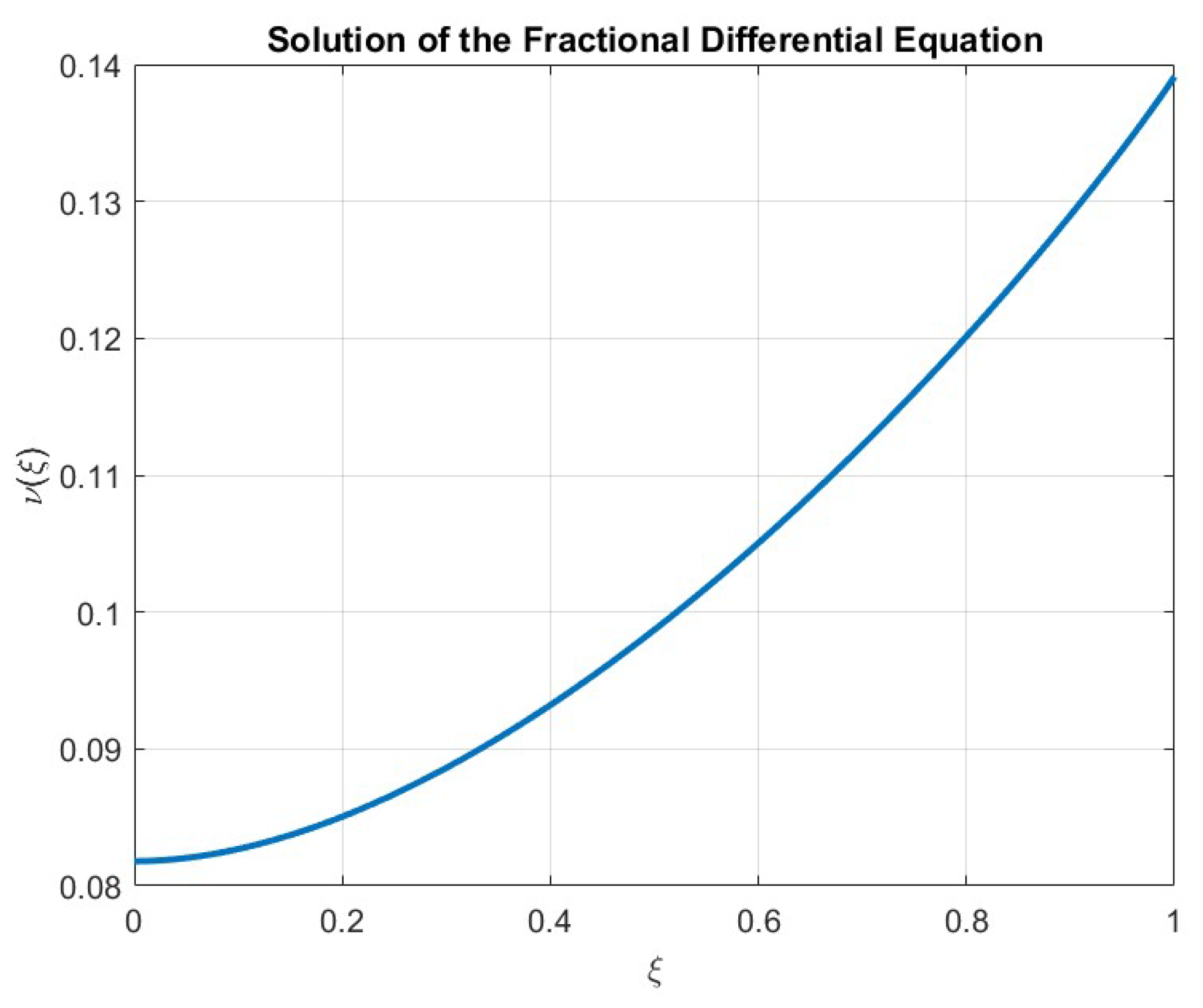
5. Example

Let us discuss the problem outlined below:

$$\begin{array}{c}\hfill \left\{\begin{array}{c}{}^{ABC}D_{0^{+}}^{{\displaystyle \frac{1}{2}}}\nu (\wp )={\displaystyle \frac{{sin}^{-1}(\wp )}{1+\frac{1}{10}|\nu (\wp \left)\right|+\frac{1}{10}|{}^{ABC}D_{0^{+}}^{{\displaystyle \frac{1}{2}}}\nu (\wp )|+\frac{1}{10}\left|\right({}^{ABC}D_{0^{+}}^{{\displaystyle \frac{1}{2}}}({}^{ABC}D_{0^{+}}^{{\displaystyle \frac{1}{2}}}\nu (\wp ))|}}+{\int }_0^1\mathfrak{X}(\wp ,\nu (\wp ))d\wp ,,\hfill \\ \nu \left(0\right)={\displaystyle \frac{1}{4}}\nu \left({\displaystyle \frac{1}{3}}\right),\wp \in [0,1].\hfill \end{array}\right.\end{array}$$

(16)

Clearly $\mathfrak{f}$, $\mathfrak{X}$ is continuous.

$$\begin{array}{cc}\hfill \mathfrak{f}(\wp ,{\nu }_1,{\nu }_2,{\nu }_3)& ={\displaystyle \frac{{sin}^{-1}(\wp )}{1+\frac{1}{10}\left|\nu \right(\wp \left)\right|+\frac{1}{10}|{}^{ABC}D_{0^{+}}^{{\displaystyle \frac{1}{2}}}\nu (\wp )|+\frac{1}{10}\left|\right({}^{ABC}D_{0^{+}}^{{\displaystyle \frac{1}{2}}}({}^{ABC}D_{0^{+}}^{{\displaystyle \frac{1}{2}}}\nu (\wp ))|}}.\hfill \\ \hfill \mathfrak{X}(\wp ,\nu (\wp \left)\right)& ={\displaystyle \frac{1}{100}}{\wp }^2\nu (\wp ).\hfill \end{array}$$

where

$$\begin{array}{c}\hfill \mathfrak{I}=[0,1]{\varsigma }^{\star }={\displaystyle \frac{1}{2}},c_1={\displaystyle \frac{1}{4}},{\wp }_1={\displaystyle \frac{1}{3}}(m=1).\end{array}$$

Now

$$\begin{array}{cc}\hfill & |\mathfrak{f}(\wp ,{\nu }_1,{\nu }_2,{\nu }_3)-\mathfrak{f}(\wp ,{\upsilon }_1,{\upsilon }_2,{\upsilon }_3)|=\hfill \\ \hfill & |{\displaystyle \frac{{sin}^{-1}(\wp )}{1+\frac{1}{10}\left|\nu \right(\wp \left)\right|+\frac{1}{10}|{}^{ABC}D_{0^{+}}^{{\displaystyle \frac{1}{2}}}\nu (\wp )|+\frac{1}{10}\left|\right({}^{ABC}D_{0^{+}}^{{\displaystyle \frac{1}{2}}}({}^{ABC}D_{0^{+}}^{{\displaystyle \frac{1}{2}}}\nu (\wp ))|}}\hfill \\ \hfill & -{\displaystyle \frac{{sin}^{-1}(\wp )}{1+\frac{1}{10}\left|\upsilon \right(t\left)\right|+\frac{1}{10}|{}^{ABC}D_{0^{+}}^{{\displaystyle \frac{1}{2}}}\upsilon (\wp )|+\frac{1}{10}\left|\right({}^{ABC}D_{0^{+}}^{{\displaystyle \frac{1}{2}}}({}^{ABC}D_{0^{+}}^{{\displaystyle \frac{1}{2}}}\upsilon (\wp ))|}}|\hfill \\ \hfill & \le {\displaystyle \frac{\pi }{20}}\left(|{\nu }_1-{\upsilon }_1|+|{\nu }_2-{\upsilon }_2|+|{\nu }_3-{\upsilon }_3|\right),\hfill \end{array}$$

and

$$\begin{array}{c}\hfill |\mathfrak{X}(\wp ,{\nu }_1(\wp ))-\mathfrak{X}(\wp ,{\upsilon }_1(\wp ))|\le {\displaystyle \frac{1}{100}}\left|\right|{\nu }_1-{\upsilon }_1\left|\right|.\end{array}$$

where $\mathbf{K}={\displaystyle \frac{\pi }{20}}$ and $\mathfrak{L}={\displaystyle \frac{1}{100}}$; the assumption ${\mathfrak{O}}_1-{\mathfrak{O}}_2$ is satisfied. Since all the conditions of Theorem 3 are satisfied and $\Delta =0.1766<1$, problem (16) has a unique solution.

Additionally, we have ${\varphi }^{*}={\displaystyle \frac{\pi }{2}}$, ${\phi }^{*}={\displaystyle \frac{1}{100}}$

$$\begin{array}{c}\hfill \Omega =0.714.<1\end{array}$$

The criteria of Theorem 4 are all satisfied; therefore, problem (16) has at least one solution. Finally, since all the requirements of Theorem 5 are satisfied, problem (16) is stable with respect to both Hyers–Ulam and generalized Hyers-Ulam stability. See Figure 1 for more details.

6. Conclusions

In this research, we investigated the existence, uniqueness, and stability of solutions to Problem (3). By employing fixed-point theorems, we explored the corresponding theoretical insights. To the best of our knowledge, this methodology has not been previously applied to such problems. Our goal was to enhance the literature by offering a thorough exploration of diverse dynamic processes and their practical applications within fractal environments. Other fractional derivatives, such as the modified Atangana–Baleanu fractional derivative in the Caputo sense (mABC), could be incorporated into the fractional boundary value problem in future studies.

References

- Podlubny, I. Fractional Differential Equations: An Introduction to Fractional Derivatives, Fractional Differential Equations, to Methods of Their Solution and Some of Their Applications; Elsevier: Amsterdam, The Netherlands, 1998. [Google Scholar]
- Samko, S.G. Fractional Integrals and Derivatives. Theory and Applications; CRC Press: Boca Raton, FL, USA, 1993. [Google Scholar]
- Kilbas, A.A.; Srivastava, H.M.; Trujillo, J.J. Theory and Applications of Fractional Differential Equations; Elsevier: Amsterdam, The Netherlands, 2006; Volume 204. [Google Scholar]
- Hilfer, R. (Ed.) Applications of Fractional Calculus in Physics; World Scientific: Singapore, 2000. [Google Scholar]
- Sun, H.; Zhang, Y.; Baleanu, D.; Chen, W.; Chen, Y. A new collection of real world applications of fractional calculus in science and engineering. Commun. Nonlinear Sci. Numer. Simul. 2018, 64, 213–231. [Google Scholar] [CrossRef]
- Magin, R.L. Fractional calculus models of complex dynamics in biological tissues. Comput. Math. Appl. 2010, 59, 1586–1593. [Google Scholar] [CrossRef]
- Sadek, L.; Lazar, T.A. On Hilfer cotangent fractional derivative and a particular class of fractional problems. AIMS Math. 2023, 8, 28334–28352. [Google Scholar] [CrossRef]
- Sadek, L. Controllability, observability, and stability of ϕ-conformable fractional linear dynamical systems. Asian J. Control 2024, 26, 2476–2494. [Google Scholar] [CrossRef]
- Sadek, L. A cotangent fractional derivative with the application. Fractal Fract. 2023, 7, 444. [Google Scholar] [CrossRef]
- Sadek, L.; Baleanu, D.; Abdo, M.S.; Shatanawi, W. Introducing novel Θ-fractional operators: Advances in fractional calculus. J. King Saud Univ.-Sci. 2024, 36, 103352. [Google Scholar] [CrossRef]
- Sadek, L.; Akgül, A. New properties for conformable fractional derivative and applications. Progr. Fract. Differ. Appl. 2024, 10, 335–344. [Google Scholar]
- Ghanbari, B.; Atangana, A. A new application of fractional Atangana-Baleanu derivatives: Designing ABC-fractional masks in image processing. Phys. A Stat. Mech. Its Appl. 2020, 542, 123516. [Google Scholar] [CrossRef]
- Bas, E.; Ozarslan, R. Real world applications of fractional models by Atangana-Baleanu fractional derivative. Chaos Solitons Fractals 2018, 116, 121–125. [Google Scholar] [CrossRef]
- Baleanu, D.; Sajjadi, S.S.; Jajarmi, A.; Defterli, Ö. On a nonlinear dynamical system with both chaotic and nonchaotic behaviors: A new fractional analysis and control. Adv. Differ. Equa. 2021, 2021, 234. [Google Scholar] [CrossRef]
- Caputo, M.; Fabrizio, M. A new definition of fractional derivative without singular kernel. Prog. Fract. Differ. Appl. 2015, 1, 73–85. [Google Scholar]
- Atangana, A.; Baleanu, D. New fractional derivatives with nonlocal and non-singular kernel: Theory and application to heat transfer model. arXiv 2016, arXiv:1602.03408. [Google Scholar] [CrossRef]
- Atangana, A. Non validity of index law in fractional calculus: A fractional differential operator with Markovian and non-Markovian properties. Phys. A Stat. Mech. Its Appl. 2018, 505, 688–706. [Google Scholar] [CrossRef]
- Atangana, A.; Gómez-Aguilar, J.F. Fractional derivatives with no-index law property: Application to chaos and statistics. Chaos Solitons Fractals 2018, 114, 516–535. [Google Scholar] [CrossRef]
- Abdeljawad, T. A Lyapunov type inequality for fractional operators with nonsingular Mittag-Leffler kernel. J. Inequalities Appl. 2017, 2017, 130. [Google Scholar] [CrossRef]
- Almalahi, M.A.; Ghanim, F.; Botmart, T.; Bazighifan, O.; Askar, S. Qualitative analysis of Langevin integro-fractional differential equation under Mittag-Leffler functions power law. Fractal Fract. 2021, 5, 266. [Google Scholar] [CrossRef]
- Almalahi, M.A.; Bazighifan, O.; Panchal, S.K.; Askar, S.S.; Oros, G.I. Analytical study of two nonlinear coupled hybrid systems involving generalized Hilfer fractional operators. Fractal Fract. 2021, 5, 178. [Google Scholar] [CrossRef]
- Sadek, L.; Akgül, A.; Bataineh, A.S.; Hashim, I. A cotangent fractional Gronwall inequality with applications. AIMS Math. 2024, 9, 7819–7833. [Google Scholar] [CrossRef]
- Bachir, F.S.; Said, A.; Benbachir, M.; Benchohra, M. Hilfer-Hadamard fractional differential equations: Existence and attractivity. Adv. Theory Nonlinear Anal. Its Appl. 2021, 5, 49–57. [Google Scholar]
- Saha, K.K.; Sukavanam, N.; Pan, S. Existence and uniqueness of solutions to fractional differential equations with fractional boundary conditions. Alex. Eng. J. 2023, 72, 147–155. [Google Scholar] [CrossRef]
- Khan, A.U.; Khan, R.U.; Ali, G.; Aljawi, S. The study of nonlinear fractional boundary value problems involving the p-Laplacian operator. Phys. Scr. 2024, 99, 085221. [Google Scholar] [CrossRef]
- Dimitrov, N.D.; Jonnalagadda, J.M. Existence, Uniqueness, and Stability of Solutions for Nabla Fractional Difference Equations. Fractal Fract. 2024, 8, 591. [Google Scholar] [CrossRef]
- González-Camus, J. Existence and uniqueness of discrete weighted pseudo S-asymptotically ω-periodic solution to abstract semilinear superdiffusive difference equation. Fract. Calc. Appl. Anal. 2025, 28, 430–452. [Google Scholar] [CrossRef]
- Gogoi, B.; Singkai, W.; Gogoi, S. 13 Existence and Uniqueness of Solution of Nonlinear Fractional Dynamic Equation Involving Initial Condition on Time Scales. In Summability, Fixed Point Theory and Generalized Integrals with Applications; Imprint Chapman and Hall/CRC: Boca Raton, FL, USA, 2025. [Google Scholar]
- Ulam, S.M. A Collection of the Mathematical Problems; Interscience Publisheres: New York, NY, USA, 1960. [Google Scholar]
- Hyers, D.H. On the stability of the linear functional equation. Proc. Natl. Acad. Sci. USA 1941, 27, 222–224. [Google Scholar] [CrossRef]
- Almalahi, M.A.; Abdo, M.S.; Panchal, S.K. Existence and Ulam-Hyers stability results of a coupled system of -Hilfer sequential fractional differential equations. Results Appl. Math. 2021, 10, 100142. [Google Scholar] [CrossRef]
- Ali, G.; Khan, R.U.; Kamran; Aloqaily, A.; Mlaiki, N. On qualitative analysis of a fractional hybrid Langevin differential equation with novel boundary conditions. Bound. Value Probl. 2024, 2024, 62. [Google Scholar] [CrossRef]
- Jarad, F.; Abdeljawad, T.; Hammouch, Z. On a class of ordinary differential equations in the frame of Atangana-Baleanu fractional derivative. Chaos Solitons Fractals 2018, 117, 16–20. [Google Scholar] [CrossRef]
- Kreyszig, E. Introductory Functional Analysis with Applications; Wiley: New York, NY, USA, 1978; Volume 1. [Google Scholar]
- Agarwal, R.P.; Meehan, M.; O’regan, D. Fixed Point Theory and Applications; Cambridge University Press: Cambridge, UK, 2001; Volume 141. [Google Scholar]
- Schauder, J. Der fixpunktsatz in funktionalraümen. Stud. Math. 1930, 2, 171–180. [Google Scholar] [CrossRef]
Disclaimer/Publisher’s Note: The statements, opinions and data contained in all publications are solely those of the individual author(s) and contributor(s) and not of MDPI and/or the editor(s). MDPI and/or the editor(s) disclaim responsibility for any injury to people or property resulting from any ideas, methods, instructions or products referred to in the content. |
© 2025 by the authors. Licensee MDPI, Basel, Switzerland. This article is an open access article distributed under the terms and conditions of the Creative Commons Attribution (CC BY) license (https://creativecommons.org/licenses/by/4.0/).
Share and Cite
Khan, R.U.; Popa, I.-L. The Existence and Stability of Integral Fractional Differential Equations. Fractal Fract. 2025, 9, 295. https://doi.org/10.3390/fractalfract9050295
Khan RU, Popa I-L. The Existence and Stability of Integral Fractional Differential Equations. Fractal and Fractional. 2025; 9(5):295. https://doi.org/10.3390/fractalfract9050295
Chicago/Turabian StyleKhan, Rahman Ullah, and Ioan-Lucian Popa. 2025. "The Existence and Stability of Integral Fractional Differential Equations" Fractal and Fractional 9, no. 5: 295. https://doi.org/10.3390/fractalfract9050295
APA StyleKhan, R. U., & Popa, I.-L. (2025). The Existence and Stability of Integral Fractional Differential Equations. Fractal and Fractional, 9(5), 295. https://doi.org/10.3390/fractalfract9050295