Qualitative Analysis and Traveling Wave Solutions of a (3 + 1)- Dimensional Generalized Nonlinear Konopelchenko-Dubrovsky-Kaup-Kupershmidt System

Abstract

This article investigates the qualitative analysis and traveling wave solutions of a (3 + 1)-dimensional generalized nonlinear Konopelchenko-Dubrovsky-Kaup-Kupershmidt system. This equation is commonly used to simulate nonlinear wave problems in the fields of fluid mechanics, plasma physics, and nonlinear optics, as well as to transform nonlinear partial differential equations into nonlinear ordinary differential equations through wave transformations. Based on the analysis of planar dynamical systems, a nonlinear ordinary differential equation is transformed into a two-dimensional dynamical system, and the qualitative behavior of the two-dimensional dynamical system and its periodic disturbance system is studied. A two-dimensional phase portrait, three-dimensional phase portrait, sensitivity analysis diagrams, Poincaré section diagrams, and Lyapunov exponent diagrams are provided to illustrate the dynamic behavior of two-dimensional dynamical systems with disturbances. The traveling wave solution of a Konopelchenko-Dubrovsky-Kaup-Kupershmidt system is studied based on the complete discriminant system method, and its three-dimensional, two-dimensional graphs and contour plots are plotted. These works can provide a deeper understanding of the dynamic behavior of Konopelchenko-Dubrovsky-Kaup-Kupershmidt systems and the propagation process of waves.

1. Introduction

In the coming year, nonlinear partial differential equations (NLPDEs) [1,2,3] can be used to simulate mathematical models from the fields of physics, chemistry, biology, engineering technology, and finance [4,5]. For example, a biological mathematical model with an NLPDE can describe the growth model of tumors. NLPDEs are commonly used in the financial field to better describe the mathematical models for pricing financial derivatives such as options and warrants. The application of NLPDEs in physics is more extensive and can be applied in every branch of physics [6,7,8,9], such as in fluid mechanics, quantum mechanics, plasma physics, etc. [10,11]. Many NLPDEs have also been used to simulate nonlinear phenomena [12,13,14] in fields such as physics, chemistry, biology, engineering and finance. The most classic equation is the Schrödinger equation [15], Drinfel’d-Sokolov-Wilson equation [16], coupled Konopelchenko-Dubrovsky model [17], Lakshmanan-Porsezian-Daniel equation [18], Chen-Lee-Liu equation [19], thin-film ferroelectric material equation [20], Ginzburg-Landau equation [21], etc. Due to the complexity and inconsistency of nonlinear problems, the study of NLPDEs is very difficult. In recent years, research on traveling wave solutions and the qualitative analysis of NLPDEs has become one of the current hotspots. Specifically, the study of Konopelchenko-Dubrovsky-Kaup-Kupershmidt (KDKK) systems [22] is a very important model.

In this paper, we consider a (3 + 1)-dimensional generalized nonlinear KDKK system with a conformable derivative as follows [23]:

$$\left\{\begin{array}{c}{r}_3{\displaystyle \frac{{\partial }^{5}u}{\partial x^5}}+r_1{\displaystyle \frac{{\partial }^{3}u}{\partial x^3}}+r_7(u{\displaystyle \frac{{\partial }^{3}u}{\partial x^3}}+{\displaystyle \frac{\partial u}{\partial x}}{\displaystyle \frac{{\partial }^{2}u}{\partial x^2}})+r_5{\displaystyle \frac{{\partial }^{3}u}{\partial x^2\partial y}}+D_t^{\alpha }u+r_8{u}^2{\displaystyle \frac{\partial u}{\partial x}}+r_6(v{\displaystyle \frac{\partial u}{\partial x}}+u{\displaystyle \frac{\partial u}{\partial y}})+r_{2}u{\displaystyle \frac{\partial u}{\partial x}}\hfill \\ +r_9{\displaystyle \frac{\partial u}{\partial z}}+r_4{\displaystyle \frac{\partial v}{\partial y}}=0,0<\alpha \le 1,\hfill \\ {\displaystyle \frac{\partial v}{\partial x}}-{\displaystyle \frac{\partial u}{\partial y}}=0,\hfill \end{array}\right.$$

(1)

where the unknown function $u=u(x,y,z,t)$ and $v=v(x,y,z,t)$ in the above equation describe the wave field in physics. For example, the wave field u is used in plasma physics, fluid mechanics, and nonlinear optics to describe the velocity of fluids, the density of plasmas, and the strength of electromagnetic fields, respectively. Here, $(x,y,z,t)$ represents three-dimensional space, and t represents the time variable. The letter $r_i$ ($i=1,2,3,\dots ,9$) represents the real parameter. $r_1$ represents the coefficient of the third-order spatial dispersion term in the x-direction. $r_2$ is the nonlinear self-interaction coefficient of the x-direction wavefield. $r_3$ is the fifth-order spatial dispersion coefficient along the x-direction. $r_4$ represents the spatial derivative coefficient of the field in the y-direction. $r_5$ is the coefficient of the third-order mixed spatial dispersion term in the x- and y-directions. $r_6$ is the coefficient that couples the wavefield u to another field v. $r_7$ represents the interaction between wave amplitudes and their spatial derivative coefficients. $r_8$ represents the coefficient of the nonlinear self-interaction term of the wavefield. $r_9$ represents the coefficient of the wave propagation term in the z-direction.

This equation is a high-dimensional extension of the well-known Kaup-Kupershmidt equation. These parameters represent different physical characteristics in different physical systems. The interaction and physical properties between the derivative and nonlinear terms in Equation (1) can be referred to in ref. [23]. When $\alpha =1$, Equation (1) becomes a KDKK system. $D_t^{\alpha }(·)$ represents the $\alpha$-order conformable derivative with respect to time t. Its definition and properties are as follows:

Definition 1 

([24]). Let $f:[0,\infty )\to \mathbf{R}$. Then, the conformable derivative of f of order α is defined as

$$D_t^{\alpha }f\left(t\right)=\underset{\epsilon \to 0}{lim}{\displaystyle \frac{f(t+\epsilon t^{1-\alpha })-f\left(t\right)}{\epsilon }},\forall t\in (0,+\infty ),\alpha \in (0,1],$$

(2)

where the function f is α-conformable differentiable at a point t if the limit in Equation (2) exists. The property of the conformal derivative is

• $D_t^{\alpha }\left(t^{\beta }\right)=\beta t^{\beta -\alpha }$, $\forall \beta \in \mathbf{R}=(-\infty .+\infty )$.
• $D_t^{\alpha }(af\left(t\right)+bf\left(t\right))=a{D}_t^{\alpha }f\left(t\right)+b{D}_t^{\alpha }g\left(t\right)$, $\forall a,b\in \mathbf{R}$.
• $D_t^{\alpha }(f\circ g)\left(t\right)=t^{1-\alpha }g{\left(t\right)}^{\alpha -1}{g}^{\prime }\left(t\right)D_t^{\alpha }{\left(f\left(t\right)\right)|}_{t=g\left(t\right)}$.

This research work provides systematic progress. In Section 2, the second-order ordinary differential equation of Equation (1) is obtained through a traveling wave transformation and rank homogeneous balance method. In Section 3, the qualitative analysis of two-dimensional dynamical systems and their disturbance systems are studied, and phase portraita, sensitivity analysis, Poincaré section diagrams, and Lyapunov exponent diagrams are drawn by using mathematical software. In Section 4, the traveling wave solutions of Equation (1) are constructed using the complete discriminant system method. In Section 5, numerical simulation diagrams of traveling wave solutions are provided. In Section 6, this study is compared with the existing literature. A simple conclusion is presented in Section 7.

2. Mathematical Derivation

In this section, we provide a wave transformation for Equation (1):

$$v=V\left(\varsigma \right),u=U\left(\varsigma \right),\varsigma =x+y+z+\lambda {\displaystyle \frac{t^{\alpha }}{\alpha }},$$

(3)

where $\lambda$ is an arbitrary constant.

Substituting Equation (3) into Equation (1), integrating $\varsigma$ once and setting the integration constant to zero yields

$$\left\{\begin{array}{c}{U}^{\prime }[\lambda +r_7{U}^{″}+U(r_{8}U+r_2+2r_{6}V)+r_9]+r_4{V}^{\prime }+r_3{U}^{\left(5\right)}+U^{‴}(r_{7}U+r_1+r_5)=0,\hfill \\ U=V.\hfill \end{array}\right.$$

(4)

By substituting the second equation of Equation (4) into the first equation of Equation (4) and integrating it once, we can obtain

$$(\lambda +r_4+r_9)U+r_3{U}^{\left(4\right)}+{\displaystyle \frac{1}{3}}{r}_8{U}^3+r_{7}U{U}^{″}+(r_1+r_5)U^{″}+({\displaystyle \frac{1}{2}}{r}_2+r_6)U^2=r_{10},$$

(5)

where $r_{10}$ is an integral constant.

According to the polynomial probing equation method for the rank homogeneous equation, the above equation for the above equation is taken as [25]

$$U^{″}=a_2{U}^2+a_{1}U+a_0,$$

(6)

where $a_2$, $a_1$, and $a_0$ are real parameters and can be given in future calculations.

Integrating both sides of Equation (6) simultaneously once again yields

$${\left(U^{\prime }\right)}^2={\displaystyle \frac{2}{3}}{a}_2{U}^3+a_1{U}^2+2a_{0}U+c,$$

(7)

where c is an integral constant.

From Equations (6) and (7), a higher-order derivative term $U^{\left(4\right)}$ can be calculated as follows:

$$U^{\left(4\right)}={\displaystyle \frac{10}{3}}{a}_2^2{U}^3+5a_1{a}_2{U}^2+(a_1^2+6a_0{a}_2)U+2c{a}_2+a_0{a}_1.$$

(8)

Substituting Equations (6)–(8) into Equation (5) yields

$$\begin{array}{cc}\hfill & a_2={\displaystyle \frac{-3r_3\pm \sqrt{9r_7^2-10r_3{r}_8}}{20r_3}},a_1=-{\displaystyle \frac{(r_1+r_5)a_2}{(1+5a_2)r_3}},a_0=-{\displaystyle \frac{\lambda +r_4+r_9+(r_1+r_5)a_1+r_3{a}_1^2}{r_7+6r_3{a}_2}},\hfill \\ \hfill & r_{10}=r_3(2c{a}_2+a_0{a}_1).\hfill \end{array}$$

(9)

3. Qualitative Analysis

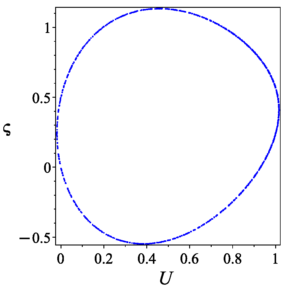
For Equation (6), we can obtain its two-dimensional dynamical system when ${\displaystyle \frac{dU}{d\varsigma }}=z$ as follows:

$$\left\{\begin{array}{c}{\displaystyle \frac{dU}{d\varsigma }}=z,\hfill \\ {\displaystyle \frac{dz}{d\varsigma }}=a_2{U}^2+a_{1}U+a_0,\hfill \end{array}\right.$$

(10)

with the Hamiltonian system

$$H(U,z)={\displaystyle \frac{1}{2}}{z}^2-{\displaystyle \frac{1}{3}}{a}_2{U}^3-{\displaystyle \frac{1}{2}}{a}_1{U}^2-a_{0}U=\hslash ,$$

(11)

where ℏ is an integral constant.

Next, let us assume that $f\left(U\right)=a_2{U}^2+a_{1}U+a_0$ and $f^{\prime }\left(U\right)=2a_{2}U+a_1$. Further, assume that $U_i$ ($i=1,2,3$) are the real roots of $f\left(U_i\right)=0$. Obviously, $(U_i,0)$ ($i=1,2,3$) are the coordinates of the equilibrium point of Equation (10). Assume that the Jacobian determinant of Equation (10) is

$$|\mathbf{J}(U_i,0)|=\left|\begin{array}{cc}0& 1\\ 2a_2{U}_i+a_1& 0\end{array}\right|=-(2a_2{U}_i+a_1)=-f^{\prime }\left(U_i\right).$$

(12)

• When ${▵}_1>0$, $f\left(U\right)=0$ has two different roots recorded as $U_1={\displaystyle \frac{-a_1+\sqrt{{\Delta }_1}}{2a_2}}$ and $U_2={\displaystyle \frac{-a_1-\sqrt{{\Delta }_1}}{2a_2}}$, $(U_1,0)$ is a saddle point and $(U_2,0)$ is center point (see Figure 1a,b), where ${▵}_1=a_1^2-4a_0{a}_2$.
• When ${▵}_1=0$, $f\left(U\right)=0$ has only one root recorded as $U_3=-{\displaystyle \frac{a_1}{2a_2}}$, and $(U_3,0)$ is a degenerate saddle point (see Figure 1c,d).

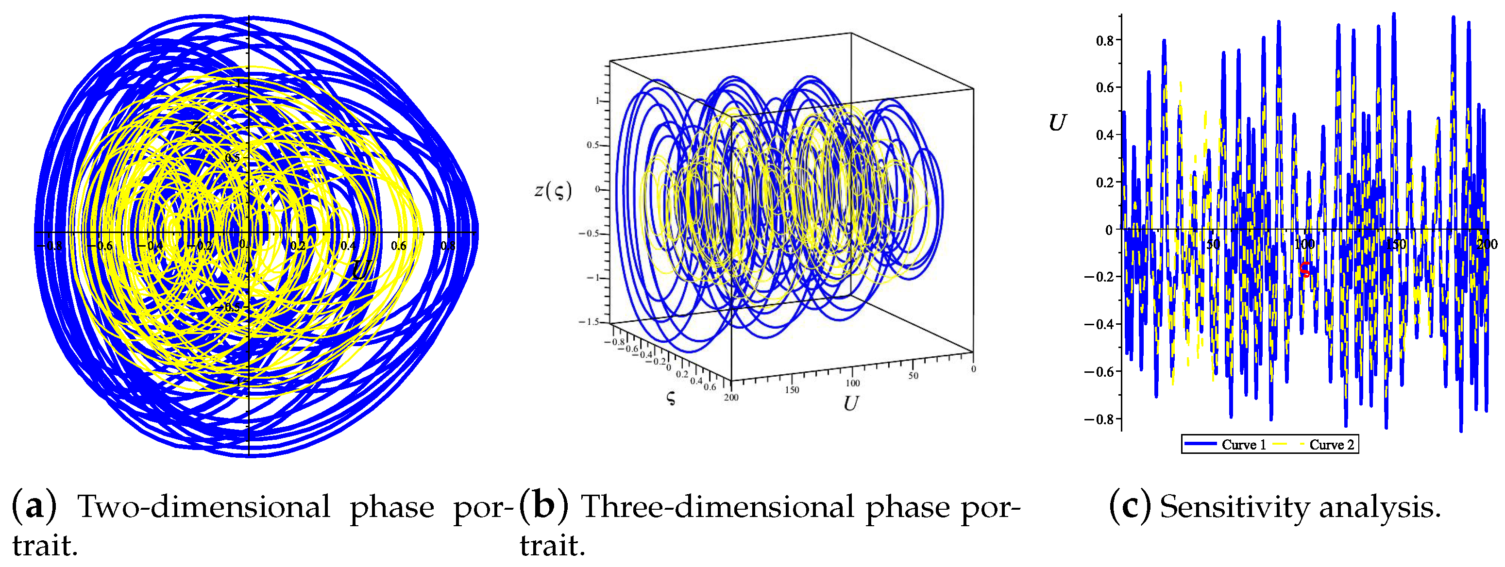
Figure 1. Phase portraits of Equation (10).

Figure 1. Phase portraits of Equation (10).

Here, we study the dynamic behavior of a perturbed system with one cycle added to Equation (10) as follows:

$$\left\{\begin{array}{c}{\displaystyle \frac{dU}{d\varsigma }}=z,\hfill \\ {\displaystyle \frac{dz}{d\varsigma }}=a_2{U}^2+a_{1}U+a_0+[A_{1}cos\left(k_1\varsigma \right)+A_{2}sin\left(k_2\varsigma \right)],\hfill \end{array}\right.$$

(13)

where $A_1$, $A_2$, $k_1$ and $k_2$ are real parameters representing amplitude and frequency, respectively.

Using mathematical software, we plot a two-dimensional phase portrait, three-dimensional phase portrait, sensitivity analysis diagram, Poincaré section diagram and Lyapunov exponent diagram of Equation (13) with different parameters, as shown in Figure 2, Figure 3 and Figure 4.

• When $a_2=2$, $a_1=-5$, $a_0=-1$, $A_1=0.38$, $k_1=0.6$, $A_2=1.5$, and $k_2=0.8$, we plot a two-dimensional phase portrait, three-dimensional phase portrait, and sensitivity analysis diagram, as shown in Figure 2. In Figure 2, the blue and yellow curves represent the phase diagram and sensitivity of the system (13) under different initial conditions, respectively. Obviously, under the parameters of the characteristics, the system exhibits chaotic behavior, and for different initial values, the system (13) is not the same.
• When $a_2=2$, $a_1=-5$, $a_0=-1$, $A_1=0.38$, $k_1=1$, $A_2=1.5$, $k_2=1$, we plot the Poincaré section diagram of Equation (13), as shown in Figure 3.
• When $a_2=2$, $a_1=-5$, $a_0=-1$, $A_1=0.38$, $k_1=0.6$, and $A_2=0$ (or $a_2=2$, $a_1=-5$, $a_0=-1$, $A_1=0$, $A_2=1.5$, and $k_2=0.8$), we plot the Lyapunov exponent diagram of Equation (13), as shown in Figure 4a (or Figure 4b). When the maximum Lyapunov exponent is greater than zero (or less than zero), the system (13) generates chaos (or stability).

4. Traveling Wave Solutions of Equation (1)

This section constructs the traveling wave solution of Equation (1) based on the complete discriminant system method of polynomials proposed by Liu (see [25]). In recent years, many studies [26] have constructed traveling wave solutions for NLPDEs using the complete discriminant system method. Here, let us recall that in the second section, we have already calculated Equation (7). Firstly, we make the following assumptions for Equation (7): $\Phi ={\left({\displaystyle \frac{2}{3}}{a}_2\right)}^{{\displaystyle \frac{1}{3}}}U$, ${\chi }_2=a_1{\left({\displaystyle \frac{2}{3}}{a}_2\right)}^{-{\displaystyle \frac{2}{3}}}$, ${\chi }_1=2a_0{\left({\displaystyle \frac{2}{3}}{a}_2\right)}^{-{\displaystyle \frac{1}{3}}}$, ${\chi }_0=c$. By substituting these conditions into Equation (7), we can obtain

$${\left({\Phi }^{\prime }\right)}^2={\Phi }^3+{\chi }_2{\Phi }^2+{\chi }_1\Phi +{\chi }_0.$$

(14)

Therefore, the integral expression of Equation (14) is

$$\pm {\left({\displaystyle \frac{2}{3}}{a}_2\right)}^{{\displaystyle \frac{1}{3}}}(\varsigma -{\varsigma }_0)=\int {\displaystyle \frac{1}{\sqrt{{\Phi }^3+{\chi }_2{\Phi }^2+{\chi }_1\Phi +{\chi }_0}}}d\Phi ,$$

(15)

where $g(\Phi )={\Phi }^3+{\chi }_2{\Phi }^2+{\chi }_1\Phi +{\chi }_0$, and the third-order complete discrimination system is

$${\Delta }_2=-27{({\displaystyle \frac{2{\chi }_2^3}{27}}+{\chi }_0-{\displaystyle \frac{{\chi }_1{\chi }_2}{3}})}^2-4{({\chi }_1-{\displaystyle \frac{{\chi }_2^2}{3}})}^3,E_1={\chi }_1-{\displaystyle \frac{{\chi }_2^2}{3}}.$$

(16)

Case 1. 

${\Delta }_2=0$, $E_1<0$

If $g(\Phi )=0$ has a double real root and a single real root, then $g(\Phi )={(\Phi -{\delta }_1)}^2(\Phi -{\delta }_2)$, where ${\delta }_1\ne {\delta }_2$. Thus, when $\Phi >{\delta }_2$, Equation (15) can be rewritten as

$$\pm (\varsigma -{\varsigma }_0)=\int {\displaystyle \frac{d\Phi }{(\Phi -{\delta }_1)\sqrt{\Phi -{\delta }_2}}}=\left\{\begin{array}{c}{\displaystyle \frac{1}{\sqrt{{\delta }_1-{\delta }_2}}}ln\left|{\displaystyle \frac{\sqrt{\Phi -{\delta }_2}-\sqrt{{\delta }_1-{\delta }_2}}{\sqrt{\Phi -{\delta }_2}+\sqrt{{\delta }_1+{\delta }_2}}}\right|,{\delta }_1>{\delta }_2,\hfill \\ {\displaystyle \frac{2}{\sqrt{{\delta }_2-{\delta }_1}}}arctan\sqrt{{\displaystyle \frac{\Phi -{\delta }_2}{{\delta }_2-{\delta }_1}}},{\delta }_1<{\delta }_2.\hfill \end{array}\right.$$

(17)

By integrating Equation (17), the traveling wave solution of Equation (1) can be obtained as follows:

$$\begin{array}{c}\hfill u_1(x,y,z,t)={({\displaystyle \frac{2}{3}}{a}_2)}^{-{\displaystyle \frac{1}{3}}}\{({\delta }_1-{\delta }_2){tanh}^2[{\displaystyle \frac{\sqrt{{\delta }_1-{\delta }_2}}{2}}{({\displaystyle \frac{2}{3}}{a}_2)}^{{\displaystyle \frac{1}{3}}}(x+y+z+\lambda {\displaystyle \frac{t^{\alpha }}{\alpha }}-{\varsigma }_0)]+{\delta }_2\},\\ \hfill {\delta }_1>{\delta }_2.\\ \hfill u_2(x,y,z,t)={({\displaystyle \frac{2}{3}}{a}_2)}^{-{\displaystyle \frac{1}{3}}}\{({\delta }_1-{\delta }_2){coth}^2[{\displaystyle \frac{\sqrt{{\delta }_1-{\delta }_2}}{2}}{({\displaystyle \frac{2}{3}}{a}_2)}^{{\displaystyle \frac{1}{3}}}(x+y+z+\lambda {\displaystyle \frac{t^{\alpha }}{\alpha }}-{\varsigma }_0)]+{\delta }_2\},\\ \hfill {\delta }_1>{\delta }_2.\\ \hfill u_3(x,y,z,t)={({\displaystyle \frac{2}{3}}{a}_2)}^{-{\displaystyle \frac{1}{3}}}\{(-{\delta }_1+{\delta }_2){tan}^2[{\displaystyle \frac{\sqrt{-{\delta }_1+{\delta }_2}}{2}}{({\displaystyle \frac{2}{3}}{a}_2)}^{{\displaystyle \frac{1}{3}}}(x+y+z+\lambda {\displaystyle \frac{t^{\alpha }}{\alpha }}-{\varsigma }_0)]+{\delta }_2\},\\ \hfill {\delta }_1<{\delta }_2.\end{array}$$

Case 2. 

${\Delta }_2=0$, $E_1=0$

If $g(\Phi )=0$ has triple real roots, then $g(\Phi )={(\Phi -\tau )}^3$. By substituting $g(\Phi )={(\Phi -\tau )}^3$ into Equation (15), the traveling wave solution of Equation (1) can be obtained as follows:

$$u_4(x,y,z,t)=[4{\left({\displaystyle \frac{2}{3}}{a}_2\right)}^{-{\displaystyle \frac{2}{3}}}{(x+y+z+\lambda {\displaystyle \frac{t^{\alpha }}{\alpha }}-{\varsigma }_0)}^{-2}+\tau ].$$

Case 3. 

${\Delta }_2>0$, $E_1<0$

If $g(\Phi )=0$ has three different real roots ${\mu }_1$, ${\mu }_2$, and ${\mu }_3$, then $g(\Phi )=(\Phi -{\mu }_1)(\Phi -{\mu }_2)(\Phi -{\mu }_3)$, where ${\mu }_1<{\mu }_2<{\mu }_3$.

When ${\mu }_1<\Phi <{\mu }_3$, a new transformation is considered:

$$\Phi ={\mu }_1+({\mu }_2-{\mu }_1){sin}^2\vartheta .$$

(18)

From Equations (17) and (18), we can obtain

$$\begin{array}{cc}\hfill \pm (\varsigma -{\varsigma }_0)& =\int {\displaystyle \frac{d\Phi }{\sqrt{g(\Phi )}}}=\int {\displaystyle \frac{2({\mu }_2-{\mu }_1)sin\vartheta cos\vartheta d\vartheta }{\sqrt{{\mu }_3-{\mu }_1}({\mu }_2-{\mu }_1)sin\vartheta cos\vartheta \sqrt{1-{\chi }^2{sin}^2\vartheta }}}\hfill \\ \hfill & ={\displaystyle \frac{2}{\sqrt{{\mu }_3-{\mu }_1}}}\int {\displaystyle \frac{d\vartheta }{\sqrt{1-{\chi }^2{sin}^2\vartheta }}},\hfill \end{array}$$

(19)

where ${\chi }^2={\displaystyle \frac{{\delta }_2-{\delta }_1}{{\delta }_3-{\delta }_1}}$.

From Equation (19), the solution of Equation (1) can be given as follows:

$$u_5(x,y,z,t)={({\displaystyle \frac{2}{3}}{a}_2)}^{-{\displaystyle \frac{1}{3}}}[{\mu }_1+({\mu }_2-{\mu }_1){\mathrm{sn}}^2({\displaystyle \frac{\sqrt{{\mu }_3-{\mu }_1}}{2}}{({\displaystyle \frac{2}{3}}{a}_2)}^{{\displaystyle \frac{1}{3}}}(x+y+z+\lambda {\displaystyle \frac{t^{\alpha }}{\alpha }}-{\varsigma }_0),\chi )].$$

(20)

When $\Phi >{\mu }_3$, we consider the transformation

$$\Phi ={\displaystyle \frac{-{\mu }_2{sin}^2\vartheta +{\mu }_3}{{cos}^2\vartheta }}.$$

Similarly, we can also provide the solutions of Equation (1) as follows:

$$u_6(x,y,z,t)={({\displaystyle \frac{2}{3}}{a}_2)}^{-{\displaystyle \frac{1}{3}}}[{\displaystyle \frac{{\mu }_3-{\mu }_2{\mathrm{sn}}^2(\frac{\sqrt{{\mu }_3-{\mu }_1}}{2}{(\frac{2}{3}{a}_2)}^{\frac{1}{3}}(x+y+z+\lambda \frac{t^{\alpha }}{\alpha }-{\varsigma }_0),\rho )}{{\mathrm{cn}}^2(\frac{\sqrt{{\mu }_3-{\mu }_1}}{2}{(\frac{2}{3}{a}_2)}^{\frac{1}{3}}(x+y+z+\lambda \frac{t^{\alpha }}{\alpha }-{\varsigma }_0),\rho )}}],$$

(21)

where ${\rho }^2={\displaystyle \frac{{\mu }_2-{\mu }_1}{{\mu }_3-{\mu }_1}}$.

Case 4. 

$\Delta <0$

If $g(\Phi )=0$ only has one root $\varkappa$, then $g(\Phi )=(\Phi -\varkappa )({\Phi }^2+p\Phi +q)$, where $p^2-4q<0$. If $\Phi >\varkappa$, we make the transformation $\Phi =\varkappa +\sqrt{{\varkappa }^2+p\varkappa +q}{tan}^2{\displaystyle \frac{\vartheta }{2}}$. From Equation (15), we can obtain

$$\begin{array}{cc}\hfill \varsigma -{\varsigma }_0& =\int {\displaystyle \frac{d\Phi }{\sqrt{(\Phi -\varkappa )({\Phi }^2+p\Phi +q)}}}=\int {\displaystyle \frac{\sqrt{{\varkappa }^2+p\varkappa +q}\frac{tan\frac{\vartheta }{2}}{{cos}^2\frac{\vartheta }{2}}d\vartheta }{{({\varkappa }^2+p\varkappa +q)}^{\frac{3}{4}}\frac{tan\frac{\vartheta }{2}}{{cos}^2\frac{\vartheta }{2}}\sqrt{1-{\varrho }^2{sin}^2\vartheta }}}\hfill \\ \hfill & ={\displaystyle \frac{1}{{({\varkappa }^2+p\varkappa +q)}^{\frac{1}{4}}}}\int {\displaystyle \frac{d\vartheta }{\sqrt{1-{\varrho }^2{sin}^2\vartheta }}},\hfill \end{array}$$

(22)

where ${\varrho }^2={\displaystyle \frac{1}{2}}(1-{\displaystyle \frac{\varkappa +\frac{p}{2}}{\sqrt{{\varkappa }^2+p\varkappa +q}}})$.

Next, we suppose that $\mathrm{cn}({({\varkappa }^2+p\varkappa +q)}^{{\displaystyle \frac{1}{4}}}(\varsigma -{\varsigma }_0),\varrho )=cos\vartheta$. Moreover, we obtain

$$cos\vartheta ={\displaystyle \frac{2\sqrt{{\varkappa }^2+p\varkappa +q}}{U-\varkappa +\sqrt{{\varkappa }^2+p\varkappa +q}}}-1.$$

(23)

When $\Phi >\varkappa$, the solutions of Equation (1) can be given as follows:

$$\begin{array}{c}\hfill u_7(x,y,z,t)={({\displaystyle \frac{2}{3}}{a}_2)}^{-{\displaystyle \frac{1}{3}}}[\varkappa +{\displaystyle \frac{2\sqrt{{\varkappa }^2+p\delta +q}}{1+\mathrm{cn}({({\varkappa }^2+p\delta +q)}^{\frac{1}{4}}{(\frac{2}{3}{a}_2)}^{-\frac{1}{3}}(x+y+z+\lambda \frac{t^{\alpha }}{\alpha }-{\varsigma }_0),\varrho )}}\\ \hfill -\sqrt{{\varkappa }^2+p\varkappa +q}].\end{array}$$

(24)

Similarly, the solutions of Equation (1) can be given as follows:

$$\begin{array}{c}\hfill u_8(x,y,z,t)={({\displaystyle \frac{2}{3}}{a}_2)}^{-{\displaystyle \frac{1}{3}}}[\vartheta +{\displaystyle \frac{2\sqrt{{\varkappa }^2+p\varkappa +q}}{1+\mathrm{cn}({({\varkappa }^2+p\varkappa +q)}^{\frac{1}{4}}{(\frac{2}{3}{a}_2)}^{-\frac{1}{3}}(x+y+z+\lambda \frac{t^{\alpha }}{\alpha }-{\varsigma }_0),\varrho )}}\\ \hfill -\sqrt{{\varkappa }^2+p\varkappa +q}].\end{array}$$

(25)

Remark 1. 

In this section, we construct the traveling wave solutions $u(x,y,z,t)$ of Equation (1). For its other solution $v(x,y,z,t)$, we can obtain it through the relationship between the traveling wave transformation (3) and Equation (4).

5. Numerical Simulation

Using mathematical software, we draw three-dimensional, two-dimensional, and contour maps of some solutions of Equation (1), as shown in Figure 5 and Figure 6. The function graph presented in Figure 5 is a hyperbolic function solution. The Jacobian function solution presented in Figure 6 indicates that it is a periodic function solution. In order to further demonstrate the influence of the conformable derivative on the solution, we plot two-dimensional graphs of different fractional-order derivatives for the same solution, as shown in Figure 5b and Figure 6b.

6. Results and Discussion

In this paper, the system of Equation (1) that is studied in this article is an NLPDE with a conformable derivative. This article uses the methods of planar dynamical system analysis and mathematical software to study the branches and phase portraits of the two-dimensional planar dynamical system of Equation (1), as well as the phase portrait, Poincaré sections, sensitivity analysis diagrams, and Lyapunov exponent diagrams of the two-dimensional planar dynamical system with periodic disturbances. These have not been reported in the existing literature. In order to further understand the propagation of waves in Equation (1) in the field of applications in physics, we use the complete discriminant system method to obtain the analytical solution of Equation (1), and we draw three-dimensional diagrams, planar diagrams, and contour diagrams. Specifically, Equation (1) becomes a KDKK system when $\alpha =1$.

7. Conclusions

In this article, we introduce the (3 + 1)-dimensional generalized nonlinear KDKK system, which is usually applied in the field of plasma physics, fluid mechanics, and nonlinear optics to describe the velocity of fluids. This article studies the dynamic behavior of two-dimensional dynamical systems and their periodic disturbance systems using the method of planar dynamical system analysis. We use mathematical software to draw the phase diagram of the two-dimensional dynamical system. Moreover, a planar phase portrait, three-dimensional phase portrait, sensitivity analysis diagrams, Poincaré section diagrams, and maximum Lyapunov exponent diagrams of two-dimensional dynamical systems with disturbances are also drawn. We draw a phase diagram, and we can easily see the saddle point and center point through the phase diagram. We can see from the performed sensitivity analysis that the graph of the same system fluctuates greatly when considering different initial values. By studying the Lyapunov exponent, we can conclude that when it is greater than zero, the system exhibits chaotic behavior. In summary, these research findings hold significant theoretical value.

References

1. Chen, D.; Shi, D.; Chen, F. Qualitative analysis and new traveling wave solutions for the stochastic Biswas-Milovic equation. AIMS Math. 2025, 10, 4092–4119. [Google Scholar] [CrossRef]
2. Zhang, K.; Cao, J.P.; Lyu, J.J. Dynamic behavior and modulation instability for a generalized nonlinear Schrödinger equation with nonlocal nonlinearity. Phys. Scr. 2025, 100, 015262. [Google Scholar] [CrossRef]
3. Sawangtong, P.; Taghipour, M.; Najafi, A. An efficient computational method for solving the fractional form of the European option price PDE with transaction cost under the fractional Heston model. Eng. Anal. Bound. Elem. 2024, 169, 105972. [Google Scholar] [CrossRef]
4. Zhang, K.; Cao, J.P. Dynamic behavior and modulation instability of the generalized coupled fractional nonlinear Helmholtz equation with cubic-quintic term. Open Phys. 2025, 23, 20250144. [Google Scholar] [CrossRef]
5. Qayyum, M.; Ahmad, E.; Tawfiq, F.M.; Salleh, S.; Saeed, S.T.; Inc, M. Series form solutions of time-space fractional Black-Scholes model via extended He-Aboodh algorithm. Alex. Eng. J. 2024, 109, 83–88. [Google Scholar] [CrossRef]
6. Merad, H.; Merghadi, F.; Merad, A. Solution of Sakata-Taketani Equation via the Caputo and Riemann-Liouville fractional derivatives. Rep. Math. Phys. 2022, 89, 359–370. [Google Scholar] [CrossRef]
7. Ishibashi, K. Riccati technique and nonoscillation of damped linear dynamic equations with the conformable derivative on time scales. Results Appl. Math. 2025, 25, 100553. [Google Scholar] [CrossRef]
8. Sadek, L.; Ldris, S.A.; Jarad, F. The general Caputo-Katugampola fractional derivative and numerical approach for solving the fractional differential equations. Alex. Eng. J. 2025, 121, 539–557. [Google Scholar] [CrossRef]
9. Yao, Z.C.; Yang, Z.W.; Gao, J.F. Unconditional stability analysis of Grünwald Letnikov method for fractional-order delay differential equations. Chaos Solitons Fract. 2023, 177, 114193. [Google Scholar] [CrossRef]
10. Zhang, Q.; Liang, Y.S. The Weyl-Marchaud fractional derivative of a type of self-affine functions. Appl. Math. Comput. 2012, 218, 8695–8701. [Google Scholar] [CrossRef]
11. Liu, X.Y.; Cai, M. Spectral deferred correction method for fractional initial value problem with Caputo-Hadamard derivative. Math. Comput. Simul. 2024, 226, 323–337. [Google Scholar] [CrossRef]
12. Odibat, Z.; Odibat, Z. On a New Modification of the Erdélyi-Kober Fractional Derivative. Fractal Fract. 2021, 5, 121. [Google Scholar] [CrossRef]
13. Li, C.Y. Zero-r law on the analyticity and the uniform continuity of fractional resolvent families. Integral Equ. Oper. Theory 2024, 96, 34. [Google Scholar]
14. Li, C.Y. The Hautus-type inequality for abstract fractional cauchy problems and its observability. J. Math. 2024, 2024, 6179980. [Google Scholar]
15. Patel, Y.F.; Izadi, M. An analytical investigation of nonlinear time-fractional Schrödinger and coupled Schrödinger-KdV equations. Results Phys. 2025, 70, 108317. [Google Scholar] [CrossRef]
16. Chen, S.Q.; Liu, Y.; Wei, L.X.; Guan, B. Exact solutions to fractional Drinfel’d-Sokolov-Wilson equations. Chin. J. Phys. 2018, 56, 708–720. [Google Scholar] [CrossRef]
17. Wang, J.; Li, Z. A dynamical analysis and new traveling wave solution of the fractional coupled Konopelchenko-Dubrovsky model. Fractal Fract. 2024, 8, 341. [Google Scholar] [CrossRef]
18. Shi, D.; Liu, C.Y.; Li, Z. New optical soliton solutions to the coupled fractional Lakshmanan-Porsezian-Daniel equations with Kerr law of nonlinearity. Results Phys. 2023, 51, 106625. [Google Scholar] [CrossRef]
19. Rahman, M.U.; AL-Essa, L.A. Explorating the solition solutions of fractional Chen-Lee-Liu equation with birefringent fibers arising in optics and their sensitive analysis. Opt. Quant. Electron. 2024, 56, 1041. [Google Scholar] [CrossRef]
20. Li, Z.; Peng, C. Bifurcation, phase portrait and traveling wave solution of time-fractional thin-film ferroelectric material equation with beta fractional derivative. Phys. Lett. A 2023, 484, 129080. [Google Scholar] [CrossRef]
21. Qi, J.M.; Li, X.W.; Bai, L.Q.; Sun, Y.Q. The exact solutions of the variable-order fractional stochastic Ginzburg-Landau equation along with analysis of bifurcation and chaotic behaviors. Chaos Solitons Fract. 2023, 175, 113946. [Google Scholar] [CrossRef]
22. Tuan, N.M.; Meesad, P. A bilinear neural network method for solving a generalized fractional (2+1)-dimensional Konopelchenko-Dubrovsky-Kaup-Kupershmidt equation. Int. J. Theor. Phys. 2025, 64, 17. [Google Scholar] [CrossRef]
23. Khater, M.M.A. Pfaffian solutions and nonlinear dynamics of surface waves in two horizontal and one vertical directions with dispersion, dissipation and nonlinearity effects. Alex. Eng. J. 2024, 108, 232–243. [Google Scholar] [CrossRef]
24. Raza, N. Exact periodic and explicit solutions the conformable time fractional Ginzburg-Landau equation. Opt. Quantum Electron. 2018, 50, 154–170. [Google Scholar] [CrossRef]
25. Liu, C.S. Applications of complete discrimination system for polynomial for classifications of traveling wave solutions to nonlinear differential equations. Comput. Phys. Commun. 2010, 181, 317–324. [Google Scholar] [CrossRef]
26. Liu, C.Y. The traveling wave solution and dynamics analysis of the fractional order generalized Pochhammer-Chree equation. AIMS Math. 2024, 9, 33956–33972. [Google Scholar] [CrossRef]
Figure 2. Phase portraits and sensitivity analysis of Equation (13).
Fractalfract 09 00285 g002
Figure 3. Poincaré section of Equation (13) for k 1 = k 2 = 1 .
Fractalfract 09 00285 g003
Figure 4. Lyapunov exponents of Equation (13).
Fractalfract 09 00285 g004
Figure 5. Traveling wave solution u 1 of Equation (1) for a 2 = 3 2 , a 1 = 3 , a 0 = c = 0 , y = z = 1 , ς 0 = 2 .
Fractalfract 09 00285 g005
Figure 6. Traveling wave solution u 5 of Equation (1) for a 2 = 3 2 , a 1 = 3 , a 0 = 1 , c = 0 , y = z = 1 , ς 0 = 2 .
Fractalfract 09 00285 g006
Disclaimer/Publisher’s Note: The statements, opinions and data contained in all publications are solely those of the individual author(s) and contributor(s) and not of MDPI and/or the editor(s). MDPI and/or the editor(s) disclaim responsibility for any injury to people or property resulting from any ideas, methods, instructions or products referred to in the content.