Discrete Memristive Hindmarsh-Rose Neural Model with Fractional-Order Differences

Abstract

Discrete systems can offer advantages over continuous ones in certain contexts, particularly in terms of simplicity and reduced computational costs, though this may vary depending on the specific application and requirements. Recently, there has been growing interest in using fractional differences to enhance discrete models’ flexibility and incorporate memory effects. This paper examines the dynamics of the discrete memristive Hindmarsh-Rose model by integrating fractional-order differences. Our results highlight the complex dynamics of the fractional-order model, revealing that chaotic firing depends on both the fractional-order and magnetic strength. Notably, certain magnetic strengths induce a transition from periodic firing in the integer-order model to chaotic behavior in the fractional-order model. Additionally, we explore the dynamics of two coupled discrete systems, finding that electrical coupling leads to the synchronization of chaotic dynamics, while chemical coupling ultimately results in a quiescent state.

1. Introduction

Mathematical neuron models are essential tools for simulating and understanding the complex firing patterns of neurons [1,2]. These models replicate the changes in action potentials that drive electrical signals, which are crucial for information transfer between neurons. By simulating neuronal signaling, they provide valuable insights into the mechanisms underlying neural activity. Over the past few decades, significant efforts have been devoted to developing and analyzing these models. Continuous-time models, such as the FitzHugh–Nagumo and Hindmarsh-Rose models, have been extensively used to investigate neuronal dynamics [3,4]. In parallel, researchers have explored discrete-time neuron models, known for their simplicity and computational efficiency. Notable examples include the Rulkov and Chialvo maps [5,6]. Some discrete models are derived by discretizing continuous models as exemplified by the two-dimensional HR neuron map proposed by Li and He [7].

Recent advancements highlight the integration of memristors into neuron models, which has opened new avenues for enhancing dynamic complexity [8,9]. Memristors, known for their memory effect, introduce richer dynamics and enable more realistic simulations. The interplay of memory and feedback mechanisms at the node level expands the repertoire of accessible dynamical regimes, which in turn has important implications for the expressive capacity of memristive networks [10,11]. Additionally, memristors facilitate the incorporation of magnetic field effects by linking electric charge to magnetic flux [12,13,14,15]. Several memristive flow-based and map-based models have emerged [14,16,17,18], including the memristive HR neuron map recently introduced by Bao et al. [19]. The studies represent the significant effect of memristors on neural behavior [20,21,22]. For example, Etémé et al. [23] demonstrated that incorporating memristors into Hindmarsh-Rose (HR) models enhances the richness of dynamical behaviors, such as firing activity, synchronization, and amplitude death, under the influence of magnetic stimulation. This work laid the groundwork for further investigations into how magnetic flux can regulate neuronal activity in networks, offering insights into the emergence of synchronous and chaotic states. Furthermore, in another study [24], they explored the phenomenon of chaos suppression and synchronization enhancement through memristive coupling, emphasizing the potential for memristors to stabilize neural systems and modulate neural synchrony. These developments reflect the evolving sophistication of neuron models, driven by innovative components like memristors.

Fractional calculus, a branch of mathematical analysis, generalizes traditional differentiation and integration to non-integer orders [25]. This extension allows for derivatives and integrals of arbitrary orders, offering greater flexibility in modeling systems with memory effects and long-term dependencies [26,27]. Unlike classical calculus, fractional calculus offers a more comprehensive framework for modeling systems characterized by memory effects and long-range dependencies [28,29]. Hence, it has been applied in diverse applications [30,31,32,33]. It excels in representing complex phenomena such as anomalous diffusion, viscoelasticity, biological systems, and fractals [34,35,36]. Its ability to capture complex behaviors has made it increasingly popular for enhancing neuronal models and networks [37,38,39]. The memory effects induced by fractional derivatives reflect biological processes such as synaptic plasticity, ion channel dynamics, neural adaptation, and anomalous diffusion in the nervous system. These phenomena are history dependent, meaning the current state of the neurons is influenced by past activity.

The superiority of fractional-order models in representing intricate neuronal dynamics has been demonstrated in recent studies [40,41,42]. Researchers have explored fractional-order variants of classical models, including the Hindmarsh-Rose (HR), FitzHugh–Nagumo (FHN), and Morris–Lecar (ML) models [43,44,45]. Additionally, fractional difference equations have been successfully applied to discrete models across various domains [46,47,48]. For example, Al-Khedhairi et al. [49] investigated a Cournot–Bertrand duopoly game using discrete fractional methods, while Ji et al. [50] introduced a novel fractional-order logistic map. Al-Qurashi [51] further analyzed the discrete fractional-order Hindmarsh-Rose neuron system. These contributions emphasize the growing importance of fractional calculus in refining mathematical models across disciplines.

In this paper, we investigate the dynamics of a discrete memristive Hindmarsh-Rose model by incorporating fractional-order differences. Our motivation stems from the desire to explore how memory effects and history dependence, naturally modeled through fractional calculus, affect the intrinsic dynamics of neural systems. While the classical HR model captures essential spiking and bursting behavior, it does not account for long-range temporal dependencies, which are biologically relevant and have been observed in neural systems. By introducing fractional-order differences, we can more realistically model neurons with memory, leading to richer and more diverse dynamics. Additionally, incorporating memristive feedback into the discrete-time fractional framework allows us to investigate how nonlinearity and history-dependent conductance interact, potentially enabling the system to access complex dynamical regimes even at lower dimensionality. The analysis reveals that the model’s complex behavior is influenced by both fractional order and magnetic strength. We present bifurcation diagrams and explore various firing patterns. Additionally, the synchronization of two neuron maps is examined through electrical and chemical synapses. Section 2 introduces the discrete memristive HR neuron model and outlines the foundational concepts of fractional difference equations, leading to the formulation of the fractional-order memristive HR model. Section 3 provides a detailed dynamical analysis, while Section 4 focuses on synchronization. Finally, our conclusions are summarized in Section 5.

2. The Model

This section describes the discrete memristive Hindmarsh-Rose (mHR) map model, discusses the basic definitions of the fractional difference, and presents the discrete fractional mHR model.

2.1. Discrete mHR Model

The memristive Hindmarsh-Rose map model is a three-dimensional neuron model, which was obtained by discretizing the flow-based model presented in [52]. The describing equations of this model, with the variables x as the membrane potential, y as the resting state, and $\phi$ as the magnetic flux, are as follows:

$$\begin{array}{cc}\hfill x(n+1)& =x\left(n\right)+\delta (y\left(n\right)-ax{\left(n\right)}^3+bx{\left(n\right)}^2-mtanh\left(\phi \left(n\right)\right)x\left(n\right)),\hfill \\ \hfill y(n+1)& =y\left(n\right)+\delta (c-dx{\left(n\right)}^2-y\left(n\right)),\hfill \\ \hfill \phi (n+1)& =\phi \left(n\right)-\delta x\left(n\right).\hfill \end{array}$$

(1)

This equation follows the discrete memristive Hindmarsh-Rose (HR) model exactly as formulated by Bao et al. in 2021 [19]. The strength of the magnetic field is shown by m. $\delta$ is the iteration step-size, usually set to $\delta =0.1$. Parameters $a,b,c$ define the nonlinear cubic dynamics of the membrane potential x, and are responsible for the generation of spiking and bursting. Parameter d controls the recovery variable y. These parameters of the model are constant and kept as $a=1$, $b=3$, $c=1$, and $d=5$.

This model can generate multiple periodic and chaotic spiking and bursting dynamics as m varies. To illustrate its rich dynamics, the bifurcation diagram of the model is shown in Figure 1. The bifurcation diagrams presented in this paper illustrate the inter-spike intervals (ISI) of the neuron as specific model parameters are varied. The ISI represents the time between consecutive spikes in the neuron’s firing pattern. A spike is detected when the membrane potential x has a peak that crosses a predefined threshold value $x_{th}=0$. By plotting the ISI against the changing parameter, the bifurcation diagram reveals transitions in neuronal behavior, allowing for a detailed examination of how the neuron’s firing dynamics evolve. Below each bifurcation diagram, its corresponding largest Lyapunov exponent is presented. Figure 1 illustrates that increasing m from 0.4 to 1.6 causes successive bifurcations from periodic dynamics (periodic spiking) to chaotic dynamics containing multiple periodic windows (chaotic spiking and chaotic bursting), and then again to periodic dynamics (periodic bursting).

2.2. Basic Definitions of Fractional Difference

The basic definitions of the fractional difference are given in this subsection.

• The definition of the forward difference operator is as follows:

  $$\begin{array}{c}\hfill \Delta f\left(n\right)=f(n+1)-f\left(n\right).\end{array}$$

  (2)
• For the function $u:N_{t_0}\to \mathbb{R}$, where $N_{t_0}=\{t_0,t_0+1,t_0+2,\cdots \}$, $t_0\in \mathbb{R}$, the discrete fractional integral is obtained as

  $$\begin{array}{c}\hfill {\Delta }_{t_0}^{-q}u\left(t\right):={\displaystyle \frac{1}{\Gamma \left(q\right)}}\sum _{S=t_0}^{t-q}{(t-\sigma \left(S\right))}^{q-1}u\left(S\right),t\in \mathbb{R}\end{array}$$

  (3)

  with the order $q>0$ and $\Gamma \left(q\right)$ being the Gamma function as follows:

  $$\begin{array}{c}\hfill \Gamma \left(q\right)={\int }_0^{+\infty }{e}^{q-1}{e}^{-t}dt.\end{array}$$

  (4)

  Also, $\sigma \left(S\right)=S+1$, and $t^{\left(q\right)}$ is defined as the falling factorial as $t^{\left(v\right)}={\displaystyle \frac{\Gamma (t+1)}{\Gamma (t+1-v)}}.$
• The Caputo-like delta difference of the function u for $q>0$ is defined as

  $$\begin{array}{c}\hfill C_{{\Delta }_{t_0}^q}\equiv {\Delta }_{t_0}^{-(M-q)}{\Delta }^{M}u\left(t\right)={\displaystyle \frac{1}{\Gamma (M-q)}}\sum _{S=t_0}^{t-(M-q)}\\ \hfill {(t-\sigma \left(S\right))}^{M-q-1}{\Delta }^{M}u\left(S\right),t\in N_{t_0+M-q}\end{array}$$

  (5)

  where $M=\lceil q\rceil$.

Theorem 1.

For the delta fractional difference equation with the following equation,

$$\begin{array}{c}\hfill {}^C\Delta _{t_0}^q=f(t+q-1,u(t+q-1)),\end{array}$$

(6)

the equivalent discrete integral equation is found as follows:

$$\begin{array}{c}\hfill u\left(t\right)=\sum _{k=0}^{M-1}{\displaystyle \frac{{(t-t_0)}^{\left(k\right)}}{k!}}{\Delta }^{k}u\left(t_0\right)+{\displaystyle \frac{1}{\Gamma \left(q\right)}}\sum _{S=t_0+M-q}^{t-q}\\ \hfill {(t-\sigma \left(S\right))}^{q-1}f(S+q-1,u(S+q-1)),t\in N_{t_0+M}\end{array}$$

(7)

where ${\Delta }^{k}u\left(t_0\right)=u_k$, $k=0,1,\cdots ,M-1$[53].

2.3. Fractional-Order mHR Model

Based on the given definitions, the difference equations of the mHR map can be described as

$$\begin{array}{cc}\hfill \Delta x& =\delta (y\left(n\right)-ax{\left(n\right)}^3+bx{\left(n\right)}^2-mtanh\left(\phi \left(n\right)\right)x\left(n\right)),\hfill \\ \hfill \Delta y& =\delta (c-dx{\left(n\right)}^2-y\left(n\right)),\hfill \\ \hfill \Delta \phi & =-\delta x\left(n\right).\hfill \end{array}$$

(8)

Using the Caputo difference operator definition and Theorem 1, the fractional-order mHR model can be rewritten to the following discrete integral equation:

$$\begin{array}{cc}\hfill x\left(t\right)& =x\left(0\right)+{\displaystyle \frac{1}{\Gamma \left(q\right)}}\sum _{S=t_0+m-q}^{t-q}{(t-S-1)}^{q-1}[\hfill \\ \hfill & \delta (y(S+q-1)-ax{(S+q-1)}^3+bx{(S+q-1)}^2\hfill \\ \hfill & -mtanh\left(\phi \right(S+q-1\left)\right)x(S+q-1))],\hfill \\ \hfill y\left(t\right)& =y\left(0\right)+{\displaystyle \frac{1}{\Gamma \left(q\right)}}\sum _{S=t_0+m-q}^{t-q}{(t-S-1)}^{q-1}[\hfill \\ \hfill & \delta (c-dx{(S+q-1)}^2-y(S+q-1))],\hfill \\ \hfill \phi \left(t\right)& =\phi \left(0\right)+{\displaystyle \frac{1}{\Gamma \left(q\right)}}\sum _{S=t_0+m-q}^{t-q}{(t-S-1)}^{q-1}\hfill \\ & [-\delta x(S+q-1\left)\right].\hfill \end{array}$$

(9)

Hence, according to the definitions given in the previous subsection, the numerical equations of the fractional-order mHR model can be given as

$$\begin{array}{cc}\hfill x\left(n\right)& =x\left(0\right)+{\displaystyle \frac{1}{\Gamma \left(q\right)}}\sum _{j=1}^n{\displaystyle \frac{\Gamma (n-j+q)}{\Gamma (n-j+1)}}\left[\delta \right(y(j-1)-a\hfill \\ \hfill & x{(j-1)}^3+bx{(j-1)}^2-mtanh\left(\phi (j-1)\right)x(j-1)\left)\right],\hfill \\ \hfill y\left(n\right)& =y\left(0\right)+{\displaystyle \frac{1}{\Gamma \left(q\right)}}\sum _{j=1}^n{\displaystyle \frac{\Gamma (n-j+q)}{\Gamma (n-j+1)}}\left[\delta \right(c-dx{(j-1)}^2\hfill \\ \hfill & -y(j-1)\left)\right],\hfill \\ \hfill \phi \left(n\right)& =\phi \left(0\right)+{\displaystyle \frac{1}{\Gamma \left(q\right)}}\sum _{j=1}^n{\displaystyle \frac{\Gamma (n-j+q)}{\Gamma (n-j+1)}}[-\delta x(j-1)].\hfill \end{array}$$

(10)

Note that the numerical solution of $x\left(n\right)$ at each time is dependent on all the past events, showing the memory incorporation.

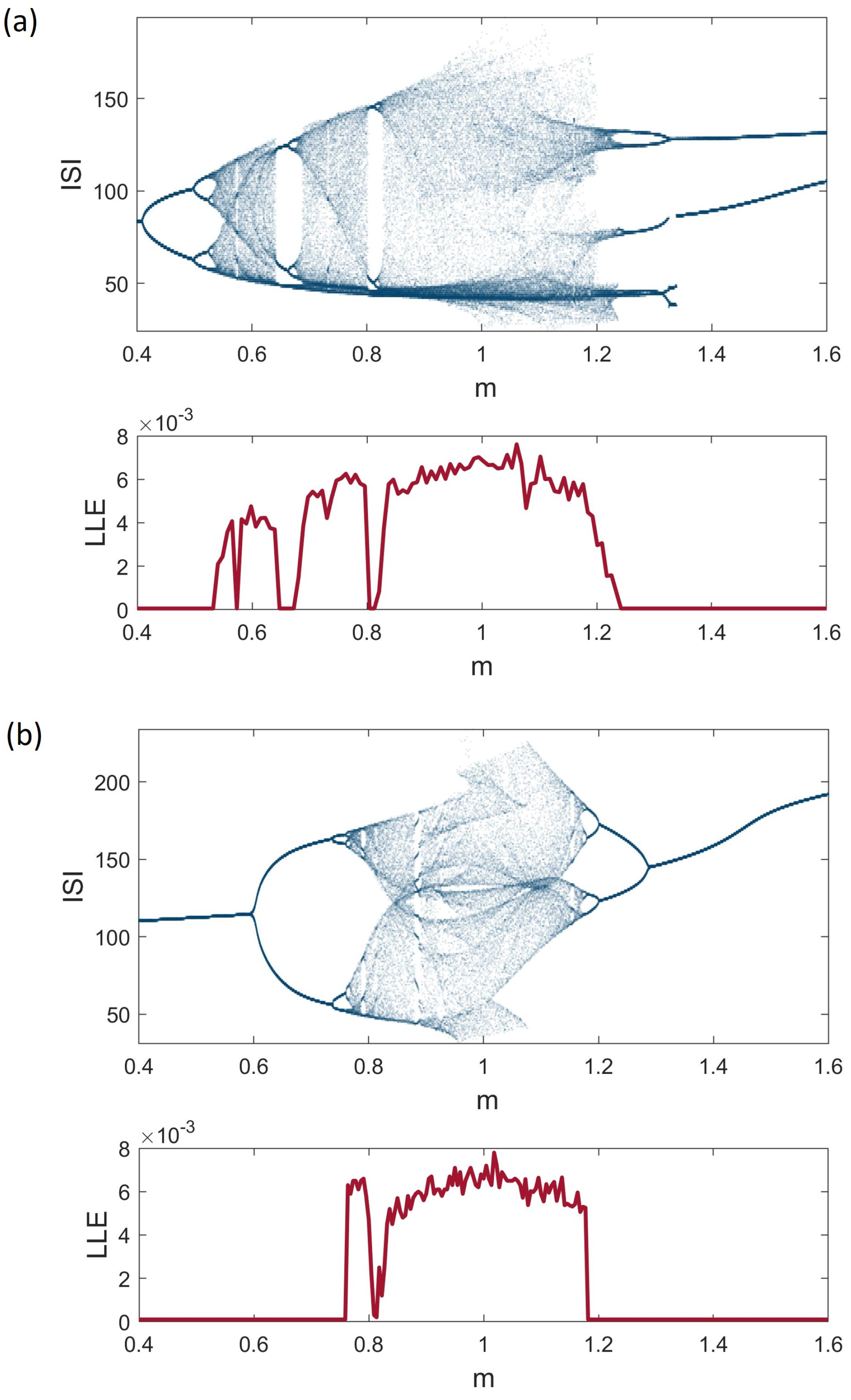
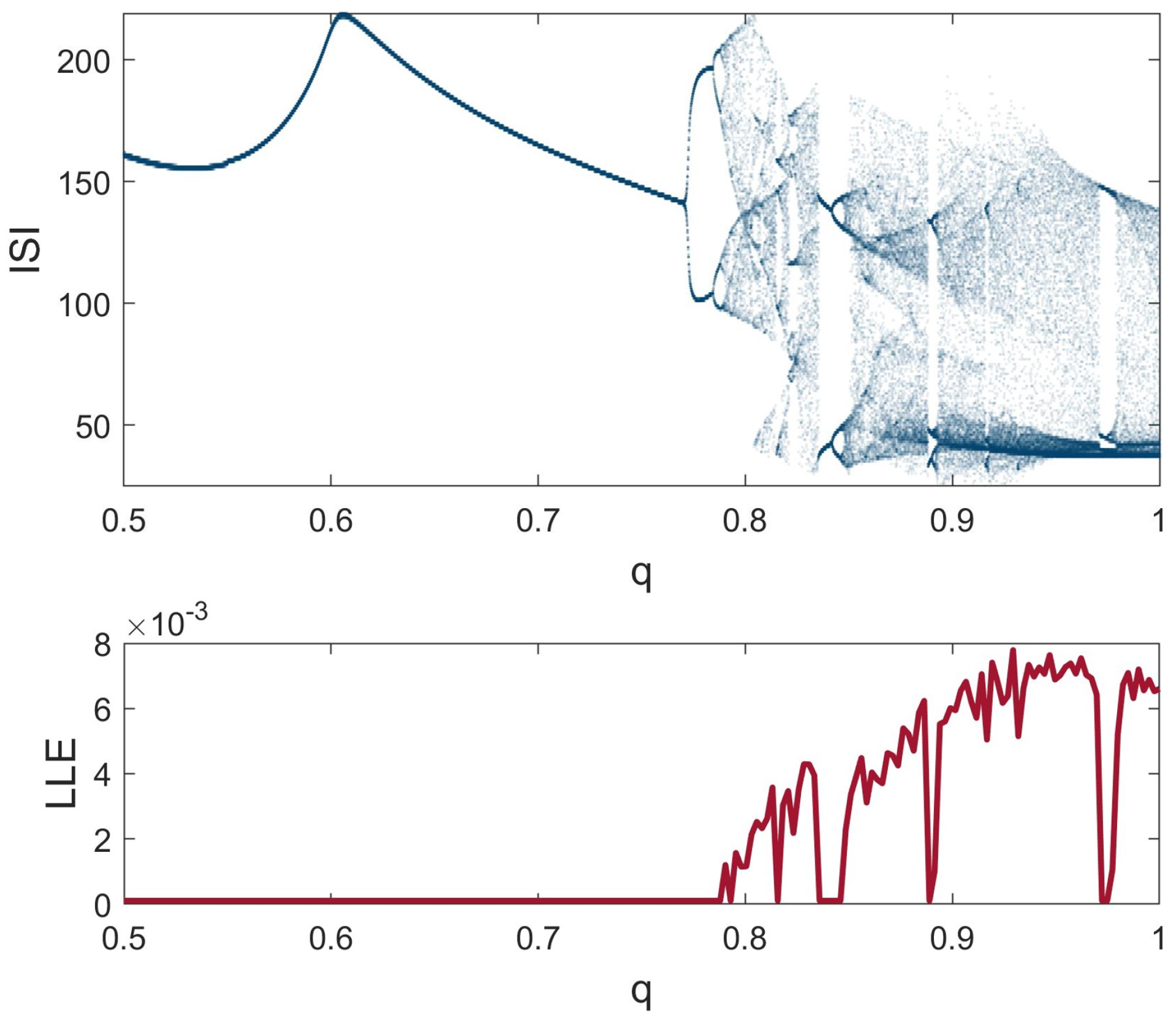
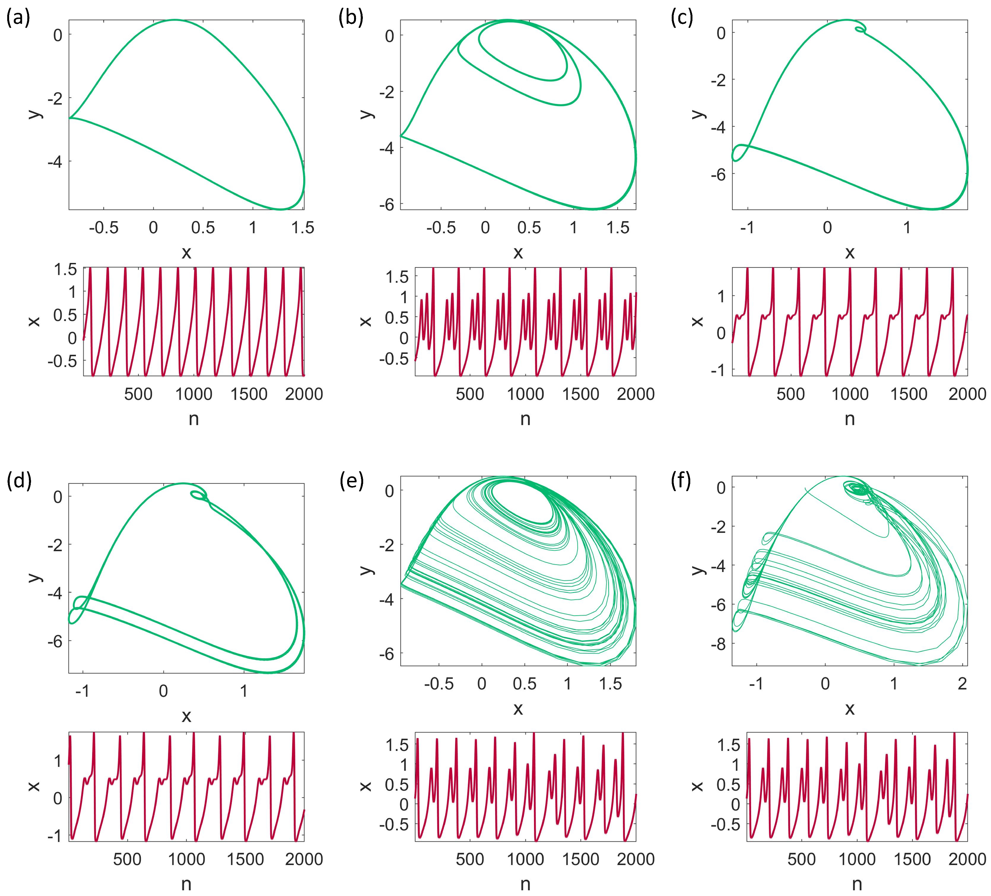
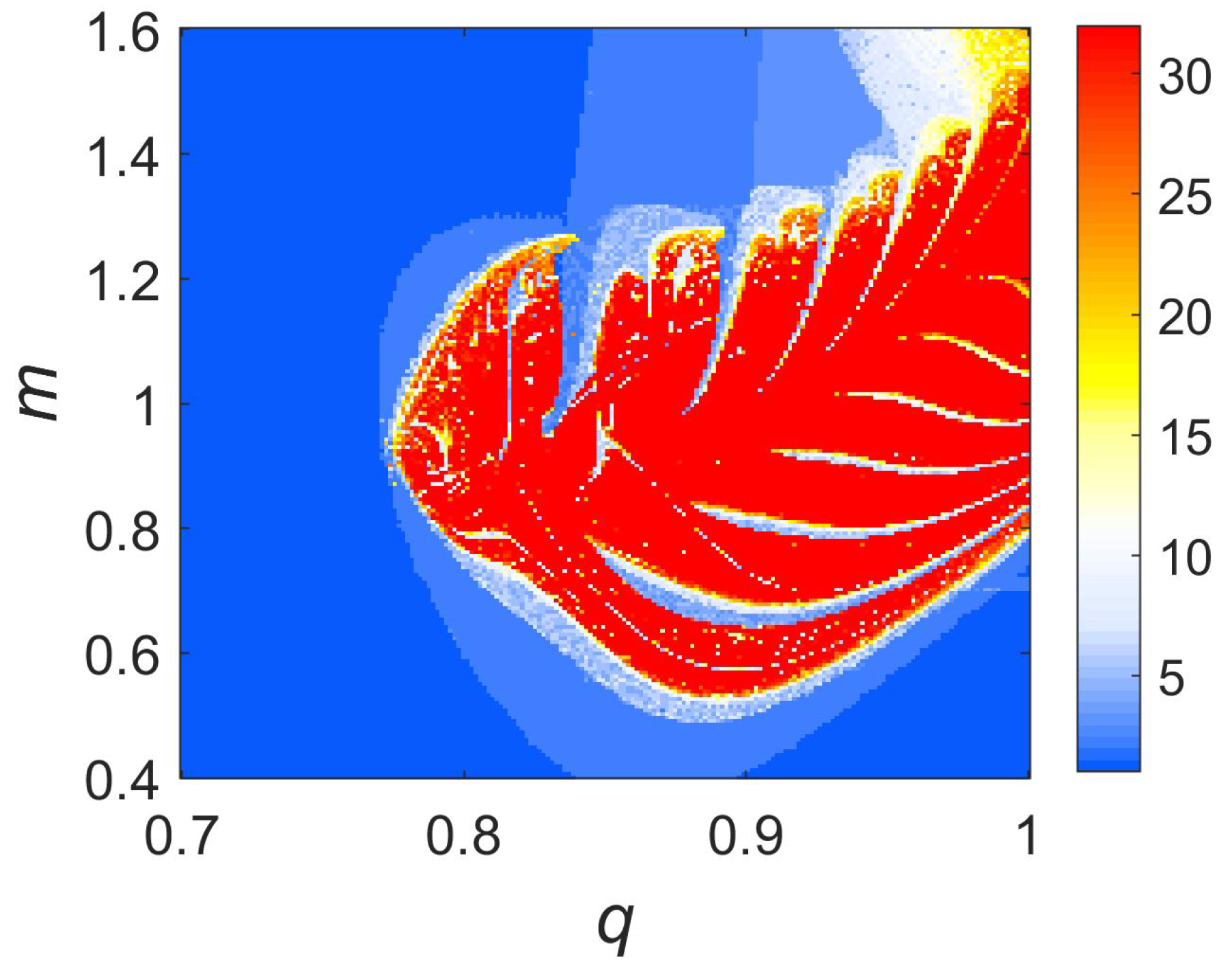
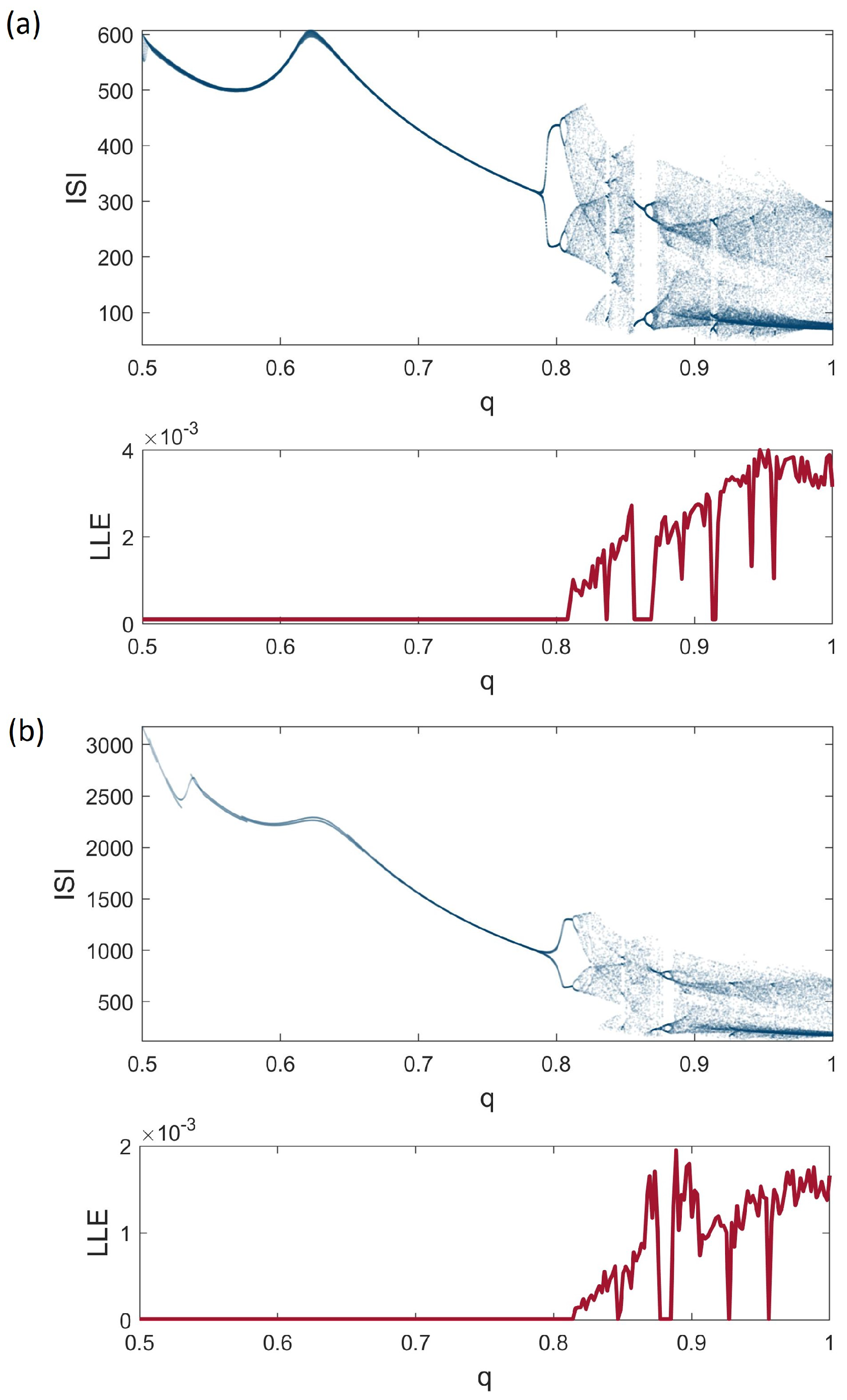
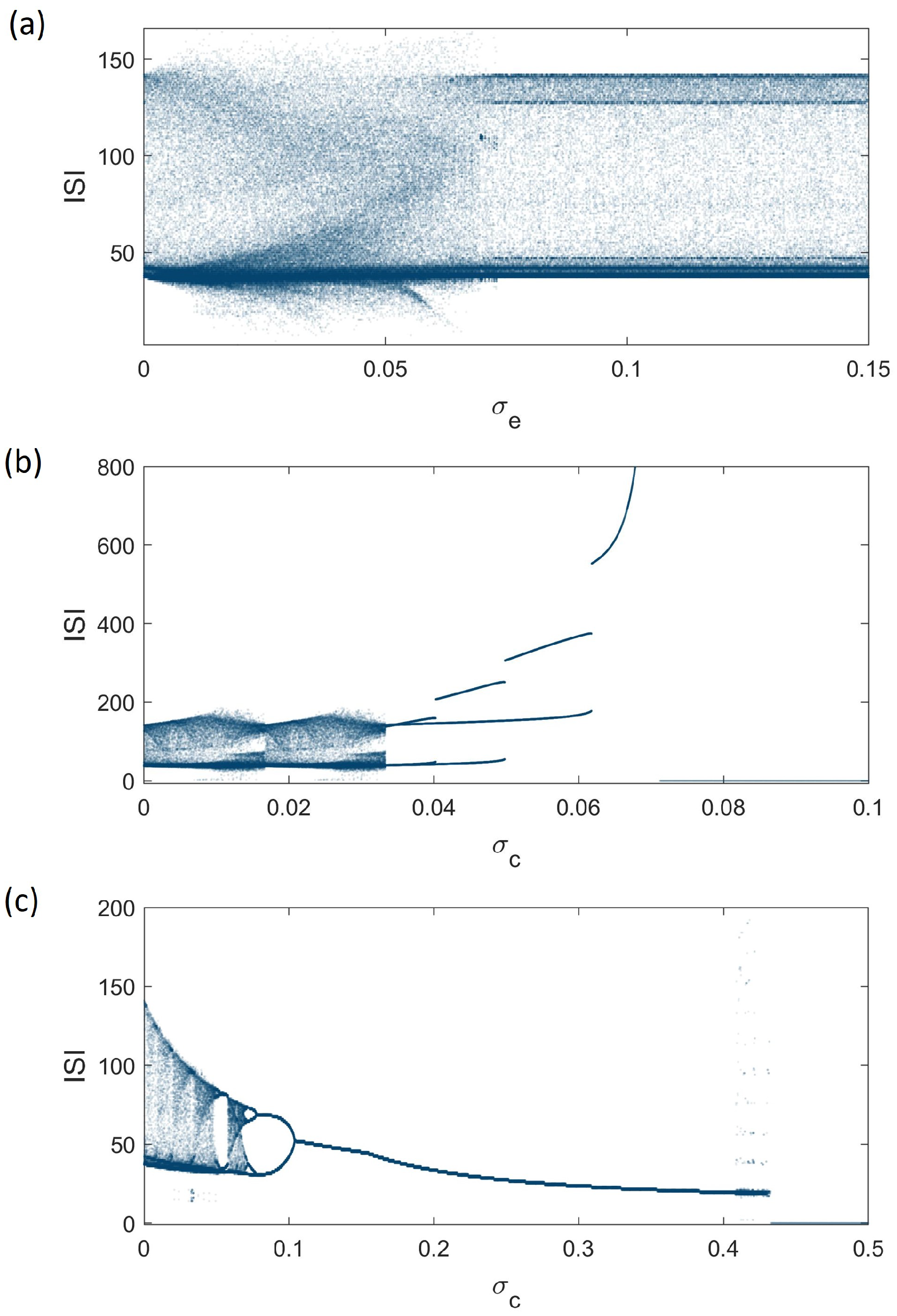
3. Dynamical Analysis

This section investigates the dynamics of the fractional-order model under different values of the fractional order and memristor strength. Figure 2 shows the bifurcation diagrams and largest Lyapunov exponent of the model for the fractional orders $q=0.9$ (Figure 2a) and $q=0.8$ (Figure 2b).

For $q=0.9$, increasing the magnetic strength causes the periodic dynamics to change to chaotic through period-doubling bifurcations. At $m=0.64$, a crisis occurs, and the chaos is converted to periodic dynamics. Another period-doubling route to chaos happens, and chaotic dynamics return. Further increases in magnetic strength lead to another crisis followed by a period-doubling route to chaos. Finally, at $m=1.23$, the chaotic dynamics disappear via period-halving bifurcations. Compared with the bifurcation diagram of the integer model, the chaotic region shifts to lower m values.

Figure 2b shows that for $q=0.8$, the chaotic region is narrower. In this diagram, the chaotic region initiates at higher m values through period-doubling bifurcations and terminates through period-halving bifurcations.

For more investigation on the effect of fractional-order, the value of m is fixed at $m=1.1$. Figure 3 represents the bifurcation diagram according to the fractional-order q. It can be observed that by decreasing q, the dynamics remain chaotic until $q=0.79$, although there exist some periodic windows. Figure 4 illustrates the attractors and time series of the fractional-order discrete memristive Hindmarsh-Rose (mHR) model for different values of the parameter m and the fractional order q. The upper panels display the phase portraits in the $x-y$ plane, while the lower panels show the corresponding time series of the variable x over discrete time steps n. Figure 4a shows periodic spiking behavior at $m=1.4$, $q=0.8$, characterized by regular and repetitive oscillations in the time series. Figure 4b exhibits periodic bursting at $m=0.66$, $q=0.9$. Figure 4c,d demonstrate a different periodic behavior, at $m=1.4$, $q=0.9$, and $m=1.27$, $q=0.9$. These patterns reveal transitions between different periodic active states in the neuron model, driven by the interplay between the fractional order and memristive feedback. In contrast, Figure 4e,f show chaotic behaviors by complex attractor structures and irregular spiking in the time domain.

Figure 5 shows the two-dimensional bifurcation diagram of the model as a function of the fractional order q and magnetic strength m. This figure is generated by computing the inter-spike intervals (ISIs), and the color bar represents the oscillation period, providing a visual representation of the system’s dynamic states across the parameter space. To detect chaotic regions, we define oscillations with periods exceeding 32 as indicative of chaotic dynamics. These regions are marked in red in the diagram. The figure illustrates that, as the fractional order decreases, the chaotic region moves towards lower magnetic strengths. Furthermore, the periodic windows become larger. Additionally, the chaotic region starts shrinking for fractional orders less than $q=0.88$. However, the fractional-order model can exhibit chaotic dynamics at values of m where the integer-order model $(q=1)$ is periodic. For example, when $m=0.6$, the integer-order model shows periodic behavior, while decreasing the derivative order (e.g., $q=0.9$) turns the dynamics chaotic.

One of the other factors affecting the dynamics of the discrete mHR model is the iteration step-size $\delta$ used in the discretization. Figure 6 shows the effect of the discretization step size on the bifurcation diagrams relative to the fractional order. While the previous analysis used $\delta =0.1$, Figure 6a uses $\delta =0.05$, and Figure 6b uses $\delta =0.02$. Figure 3 demonstrates that the chaotic region begins at $q=0.79$ when $\delta =0.1$; however, Figure 6 shows that when $\delta$ is lower, the chaotic region starts at a higher fractional order; $q=0.81$ for $\delta =0.05$, and $q=0.82$ for $\delta =0.02$. Additionally, another difference is in the ISI value in period-1 behavior for lower fractional orders. It can be observed that the ISI value increases as the $\delta$ value decreases.

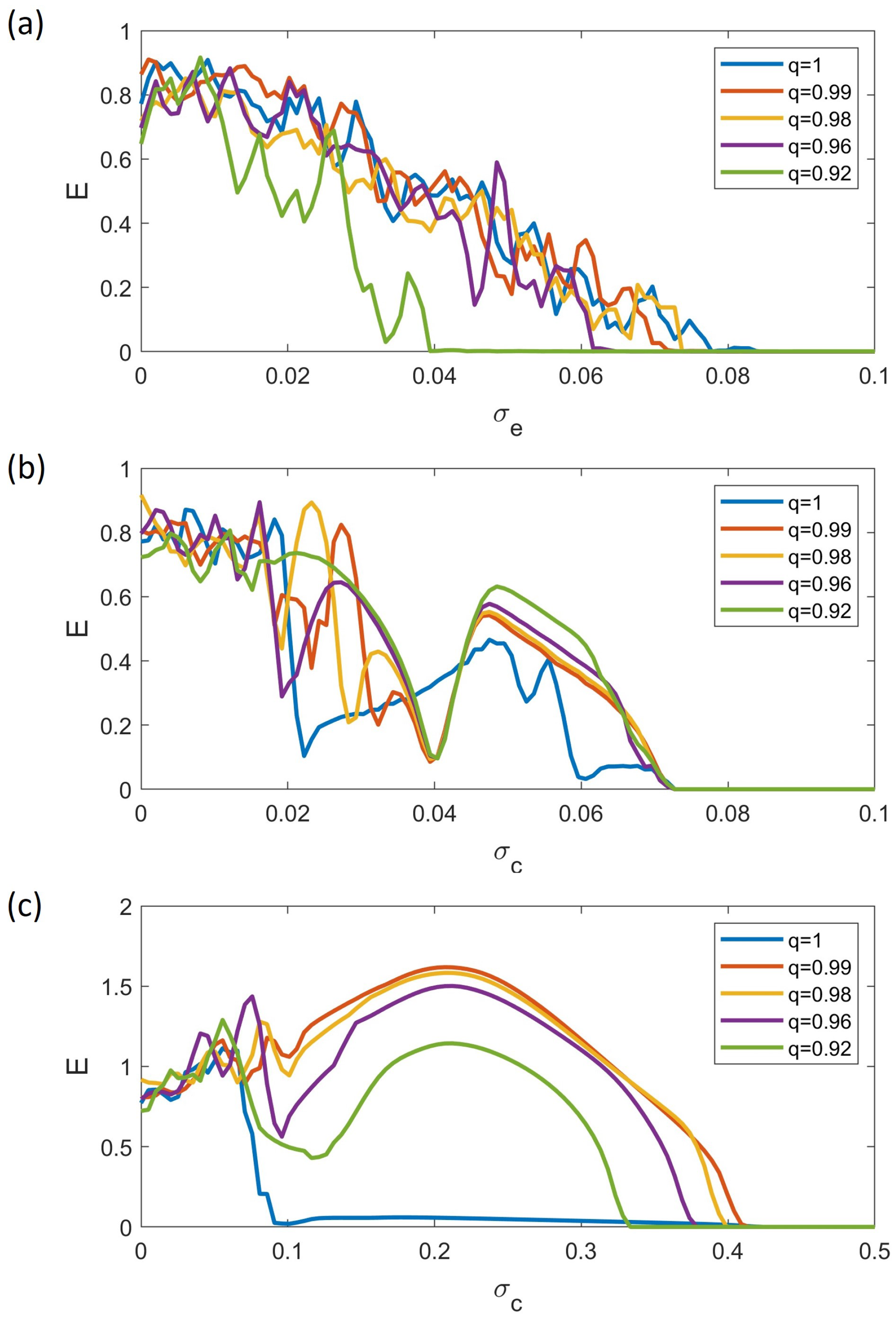
4. Synchronization Analysis

In neuroscience, synchronization among neurons is associated with various cognitive processes such as attention, perception, and memory. Abnormal synchronization, on the other hand, has been linked to neurological disorders such as epilepsy and Parkinson’s disease. In artificial systems, synchronization has also essential role. For instance, synchronized spiking in neuromorphic architectures can enable efficient communication and processing. Systems designed to mimic biological neural synchronization can potentially lead to more powerful and energy-efficient computing frameworks. As well, synchronization can serve as a mechanism for encoding and transmitting information across different regions in a network. Therefore, studying synchronization in discrete fractional-order memristive systems provides insight into how memory and feedback mechanisms can influence coordination in networks, which is relevant for both understanding biological neural dynamics and designing advanced neuromorphic systems.

Here, we investigate the behavior of two coupled fractional-order mHR discrete models. For electrical coupling, the coupling term can be defined as $h(x_1,x_2)={\sigma }_e(x_2\left(n\right)-x_1\left(n\right))$, with ${\sigma }_e$ denoting the electrical coupling strength. For the chemical coupling, the coupling term is introduced as $h(x_1,x_2)={\sigma }_c(v_s-x_1\left(n\right)){\Gamma }_c\left(x_2\left(n\right)\right)$, where ${\Gamma }_c\left(x\right)={\displaystyle \frac{1}{1+e^{-k(x-{\theta }_s)}}}$ and ${\sigma }_c$ is the chemical coupling strength. The parameters for chemical coupling are set to ${\theta }_s=-1.4$, $k=50$, $v_s=-1.4$ for the inhibitory synapse and $v_s=1.4$ for the excitatory synapse. The equations of the coupled neurons are presented in Appendix A.

To measure the synchronization of two neurons, the synchronization error is calculated as follows:

$$\begin{array}{c}\hfill E={\displaystyle \frac{1}{N}}\sum _{n=1}^N\sqrt{{(x_1\left(n\right)-x_2\left(n\right))}^2},\end{array}$$

(11)

where N is the sample size of the time series after the transient time. This measure calculates the average absolute difference between corresponding state variables over time, providing insight into how closely the systems’ behaviors align [54].

To better understand the dynamics of the coupled systems, bifurcation diagrams based on coupling strength are calculated. Figure 7a shows the bifurcation diagram of coupled systems according to the electrical coupling strength, Figure 7b refers to the inhibitory chemical coupling strength, and Figure 7c is according to the excitatory chemical coupling strength. When the coupling is electrical, the dynamics of the systems are chaotic either before synchronization ($\sigma <0.073$) or after reaching synchronization ($\sigma >0.073$). For the inhibitory chemical coupling, the systems behave asynchronously and chaotically in $\sigma <0.033$. Then, the dynamics change to periodic. The ISI of oscillations also increases as the coupling strength grows. Finally, both systems reach a quiescent state at $\sigma >0.071$. In the case of excitatory chemical coupling, the neurons have chaotic behaviors in small coupling strengths. As the coupling strength increases the chaotic dynamics are transferred to the periodic dynamics through period-halving bifurcation. The periodic dynamics remain until ${\sigma }_c=0.407$. Then, there is a small chaotic region in $0.407<{\sigma }_c<0.431$, beyond which the oscillation death occurs.

The synchronization errors of the coupled maps as a function of coupling strength for various fractional orders are shown in Figure 8. The magnetic strength is set to $m=1.1$. Figure 8a, which refers to electrical coupling, shows that synchronization depends on the fractional order, and the coupling strength threshold decreases as the fractional order decreases. For example, at $q=0.98$ and $q=0.99$, synchronization is achieved at ${\sigma }_e=0.073$, while for $q=0.96$ it is ${\sigma }_e=0.064$, and for $q=0.94$ it decreases to ${\sigma }_e=0.048$. In contrast, for inhibitory chemical coupling (Figure 8b), the synchronization error approaches zero at ${\sigma }_c>0.072$ and is almost independent of the fractional order. However, an analysis of the system dynamics for these coupling parameters shows that the systems are not synchronized in oscillating mode but reach a common quiescent state. In Figure 8c, the synchronization error for the excitatory chemical coupling is presented. The coupling strength in which the synchronization error decays to zero is dependent on the fractional-order and decreases as the fractional-order decreases. Similar to the inhibitory coupling, the zero error shows an oscillation death of systems.

5. Conclusions

This paper investigated the fractional-order discrete memristive Hindmarsh-Rose (mHR) model. In general, discrete models have several key advantages. Discrete models avoid the need for solving differential equations and can be directly mapped onto computational platforms using difference equations, making them more efficient for large-scale simulations without facing the stiffness issues or high computational costs. Also, discrete systems, particularly when extended with fractional-order operators, can exhibit rich and sometimes distinct dynamical behavior not always captured by their continuous counterparts. In this study, we examined the discrete memristive Hindmarsh-Rose model by incorporating fractional-order differences, which integrate memory effects and enhance the system’s dynamics.

Our bifurcation analysis revealed that fractional-order differences introduce additional complexity and enrich the dynamical landscape of the discrete memristive HR model. Similar to the results of Etémé et al. [24], we observed that increasing the memristor strength can suppress chaotic dynamics and enhance synchronization, suggesting that memristors could serve as effective regulators of neural synchrony in coupled systems. The inclusion of fractional-order derivatives further amplified these effects by capturing memory and hereditary properties inherent in biological neurons, which aligns with the observations of Etémé et al. [23] on long-range temporal dependencies induced by electromagnetic stimulation. In particular, our bifurcation diagrams indicated lowering the order effectively allows long-range history dependence to accumulate in the system, which in turn destabilizes periodic behavior and enables early onset of chaos—even at lower memristive gain. This kind of behavior has been described in continuous-time fractional systems, but it is rarely shown as clearly in a discrete framework. In fact, memory and feedback modulate complexity in this way, without increasing the system’s dimensionality. Also, the fractional-order model can exhibit chaos at certain magnetic strengths, where the integer-order model remains periodic. We also assessed the impact of the iteration step-size of discretization, finding that a higher fractional order is required to exhibit chaos when the iteration step size is reduced.

Furthermore, we explored the dynamics of two coupled fractional-order mHR models. Our findings demonstrated that electrically coupled neurons can achieve synchronization, with the required coupling strength being dependent on the fractional order. In contrast, chemically coupled neurons failed to synchronize; instead, they were asynchronous and ultimately reached a quiescent state as the coupling strength increased. A potential direction for future research is to complement the qualitative and bifurcation-based analysis presented here with quantitative complexity measures, such as recurrence quantification analysis or entropy-based metrics, to more precisely characterize the richness of the observed dynamical regimes.

References

1. Fortuna, L.; Buscarino, A. Spiking neuron mathematical models: A compact overview. Bioengineering 2023, 10, 174. [Google Scholar] [CrossRef] [PubMed]
2. Oliveri, H.; Goriely, A. Mathematical models of neuronal growth. Biomech. Model. Mechanobiol. 2022, 21, 89–118. [Google Scholar] [CrossRef] [PubMed]
3. FitzHugh, R. Mathematical models of threshold phenomena in the nerve membrane. Bull. Math. Biophys. 1955, 17, 257–278. [Google Scholar] [CrossRef]
4. Hindmarsh, J.L.; Rose, R. A model of neuronal bursting using three coupled first order differential equations. Proc. R. Soc. B 1984, 221, 87–102. [Google Scholar]
5. Rulkov, N.F. Modeling of spiking-bursting neural behavior using two-dimensional map. Phys. Rev. E 2002, 65, 041922. [Google Scholar] [CrossRef]
6. Chialvo, D.R. Generic excitable dynamics on a two-dimensional map. Chaos Solitons Fractals 1995, 5, 461–479. [Google Scholar] [CrossRef]
7. Li, B.; He, Z. Bifurcations and chaos in a two-dimensional discrete Hindmarsh–Rose model. Nonlinear Dyn. 2014, 76, 697–715. [Google Scholar] [CrossRef]
8. Xu, Q.; Wang, K.; Shan, Y.; Wu, H.; Chen, M.; Wang, N. Dynamical effects of memristive electromagnetic induction on a 2D Wilson neuron model. Cognit. Neurodyn. 2024, 18, 645–657. [Google Scholar] [CrossRef]
9. Xu, Q.; Huang, L.; Wang, N.; Bao, H.; Wu, H.; Chen, M. Initial-offset-boosted coexisting hyperchaos in a 2D memristive Chialvo neuron map and its application in image encryption. Nonlinear Dyn. 2023, 111, 20447–20463. [Google Scholar] [CrossRef]
10. Caravelli, F.; Sheldon, F.C.; Traversa, F.L. Global minimization via classical tunneling assisted by collective force field formation. Sci. Adv. 2021, 7, eabh1542. [Google Scholar] [CrossRef]
11. Barrows, F.; Lin, J.; Caravelli, F.; Chialvo, D.R. Uncontrolled Learning: Codesign of Neuromorphic Hardware Topology for Neuromorphic Algorithms. Adv. Intell. Syst. 2024; early view. [Google Scholar] [CrossRef]
12. Wu, F.; Ma, J.; Zhang, G. A new neuron model under electromagnetic field. Appl. Math. Comput. 2019, 347, 590–599. [Google Scholar] [CrossRef]
13. Zhang, Y.; Xu, Y.; Yao, Z.; Ma, J. A feasible neuron for estimating the magnetic field effect. Nonlinear Dyn. 2020, 102, 1849–1867. [Google Scholar] [CrossRef]
14. Ge, M.; Jia, Y.; Xu, Y.; Yang, L. Mode transition in electrical activities of neuron driven by high and low frequency stimulus in the presence of electromagnetic induction and radiation. Nonlinear Dyn. 2018, 91, 515–523. [Google Scholar] [CrossRef]
15. Yu, F.; Zhang, W.; Xiao, X.; Yao, W.; Cai, S.; Zhang, J.; Wang, C.; Li, Y. Dynamic analysis and FPGA implementation of a new, simple 5D memristive hyperchaotic Sprott-C system. Mathematics 2023, 11, 701. [Google Scholar] [CrossRef]
16. Ding, X.; Feng, C.; Wang, N.; Liu, A.; Xu, Q. Fast-slow dynamics in a memristive ion channel-based bionic circuit. Cognit. Neurodyn. 2024, 18, 3901–3913. [Google Scholar] [CrossRef]
17. Wu, F.; Hu, X.; Ma, J. Estimation of the effect of magnetic field on a memristive neuron. Appl. Math. Comput. 2022, 432, 127366. [Google Scholar] [CrossRef]
18. Xie, Y.; Ye, Z.; Li, X.; Wang, X.; Jia, Y. A novel memristive neuron model and its energy characteristics. Cognit. Neurodyn. 2024, 18, 1989–2001. [Google Scholar] [CrossRef]
19. Bao, H.; Hua, Z.; Liu, W.; Bao, B. Discrete memristive neuron model and its interspike interval-encoded application in image encryption. Sci. China Technol. Sci. 2021, 64, 2281–2291. [Google Scholar] [CrossRef]
20. Tang, D.; Wang, C.; Lin, H.; Yu, F. Dynamics analysis and hardware implementation of multi-scroll hyperchaotic hidden attractors based on locally active memristive Hopfield neural network. Nonlinear Dyn. 2024, 112, 1511–1527. [Google Scholar] [CrossRef]
21. Wang, C.; Tang, D.; Lin, H.; Yu, F.; Sun, Y. High-dimensional memristive neural network and its application in commercial data encryption communication. Expert Syst. Appl. 2024, 242, 122513. [Google Scholar] [CrossRef]
22. Lin, H.; Wang, C.; Yu, F.; Hong, Q.; Xu, C.; Sun, Y. A triple-memristor Hopfield neural network with space multistructure attractors and space initial-offset behaviors. IEEE Trans. Comput. Aided Des. Integr. Circuits Syst. 2023, 42, 4948–4958. [Google Scholar] [CrossRef]
23. Etémé, A.S.; Tabi, C.B.; Mohamadou, A. Firing and synchronization modes in neural network under magnetic stimulation. Commun. Nonlinear Sci. Numer. Simul. 2019, 72, 432–440. [Google Scholar] [CrossRef]
24. Etémé, A.S.; Tabi, C.B.; Beyala Ateba, J.F.; Ekobena Fouda, H.P.; Mohamadou, A.; Crépin Kofané, T. Chaos break and synchrony enrichment within Hindmarsh-Rose-type memristive neural models. Nonlinear Dyn. 2021, 105, 785–795. [Google Scholar] [CrossRef]
25. Gutiérrez, R.E.; Rosário, J.M.; Tenreiro Machado, J. Fractional order calculus: Basic concepts and engineering applications. Math. Probl. Eng. 2010, 2010. [Google Scholar] [CrossRef]
26. Dalir, M.; Bashour, M. Applications of fractional calculus. Appl. Math. Sci. 2010, 4, 1021–1032. [Google Scholar]
27. Danca, M.F.; Chen, G. Bifurcation and Chaos in Fractional-Order Systems; MDPI: Basel, Switzerland, 2021. [Google Scholar]
28. Rahimy, M. Applications of fractional differential equations. Appl. Math. Sci. 2010, 4, 2453–2461. [Google Scholar]
29. He, S.; Wang, H.; Sun, K. Solutions and memory effect of fractional-order chaotic system: A review. Chin. Phys. B 2022, 31, 060501. [Google Scholar] [CrossRef]
30. Jin, T.; Xia, H.; Deng, W.; Li, Y.; Chen, H. Uncertain fractional-order multi-objective optimization based on reliability analysis and application to fractional-order circuit with caputo type. Circuits Syst. Signal Process. 2021, 40, 5955–5982. [Google Scholar] [CrossRef]
31. Jin, T.; Sun, Y.; Zhu, Y. Time integral about solution of an uncertain fractional order differential equation and application to zero-coupon bond model. Appl. Math. Comput. 2020, 372, 124991. [Google Scholar] [CrossRef]
32. Liu, W.; Dai, G. Multiple solutions for a fractional nonlinear Schrödinger equation with local potential. Commun. Pure Appl. Anal. 2017, 16. [Google Scholar] [CrossRef]
33. Yu, F.; Zhang, W.; Xiao, X.; Yao, W.; Cai, S.; Zhang, J.; Wang, C.; Li, Y. Dynamic analysis and field-programmable gate array implementation of a 5D fractional-order memristive hyperchaotic system with multiple coexisting attractors. Fractal Fract. 2024, 8, 271. [Google Scholar] [CrossRef]
34. Adolfsson, K.; Enelund, M.; Olsson, P. On the fractional order model of viscoelasticity. Mech. Time-Depend. Mater. 2005, 9, 15–34. [Google Scholar] [CrossRef]
35. Sierociuk, D.; Skovranek, T.; Macias, M.; Podlubny, I.; Petras, I.; Dzielinski, A.; Ziubinski, P. Diffusion process modeling by using fractional-order models. Appl. Math. Comput. 2015, 257, 2–11. [Google Scholar] [CrossRef]
36. Wu, G.C.; Luo, M.; Huang, L.L.; Banerjee, S. Short memory fractional differential equations for new memristor and neural network design. Nonlinear Dyn. 2020, 100, 3611–3623. [Google Scholar] [CrossRef]
37. Song, C.; Cao, J. Dynamics in fractional-order neural networks. Neurocomputing 2014, 142, 494–498. [Google Scholar] [CrossRef]
38. Yan, B.; Parastesh, F.; He, S.; Rajagopal, K.; Jafari, S.; Perc, M. Interlayer and intralayer synchronization in multiplex fractional-order neuronal networks. Fractals 2022, 30, 2240194. [Google Scholar] [CrossRef]
39. Rajagopal, K.; Parastesh, F.; Abdolmohammadi, H.R.; Jafari, S.; Perc, M.; Klemenčič, E. Effects of coupling on extremely multistable fractional-order systems. Chin. J. Phys. 2024, 87, 246–255. [Google Scholar] [CrossRef]
40. Brandibur, O.; Kaslik, E. Stability properties of a two-dimensional system involving one Caputo derivative and applications to the investigation of a fractional-order Morris–Lecar neuronal model. Nonlinear Dyn. 2017, 90, 2371–2386. [Google Scholar] [CrossRef]
41. Jun, D.; Guang-Jun, Z.; Yong, X.; Hong, Y.; Jue, W. Dynamic behavior analysis of fractional-order Hindmarsh–Rose neuronal model. Cognit. Neurodyn. 2014, 8, 167–175. [Google Scholar] [CrossRef]
42. Mondal, A.; Sharma, S.K.; Upadhyay, R.K.; Mondal, A. Firing activities of a fractional-order FitzHugh-Rinzel bursting neuron model and its coupled dynamics. Sci. Rep. 2019, 9, 15721. [Google Scholar] [CrossRef] [PubMed]
43. Shi, M.; Wang, Z. Abundant bursting patterns of a fractional-order Morris–Lecar neuron model. Commun. Nonlinear Sci. Numer. Simul. 2014, 19, 1956–1969. [Google Scholar] [CrossRef]
44. Yao, Z.; Sun, K.; He, S. Firing patterns in a fractional-order FithzHugh–Nagumo neuron model. Nonlinear Dyn. 2022, 110, 1807–1822. [Google Scholar] [CrossRef]
45. Yu, Y.; Shi, M.; Kang, H.; Chen, M.; Bao, B. Hidden dynamics in a fractional-order memristive Hindmarsh–Rose model. Nonlinear Dyn. 2020, 100, 891–906. [Google Scholar] [CrossRef]
46. Atıcı, F.M.; Şengül, S. Modeling with fractional difference equations. J. Math. Anal. Appl. 2010, 369, 1–9. [Google Scholar] [CrossRef]
47. Danca, M.F. Symmetry-breaking and bifurcation diagrams of fractional-order maps. Commun. Nonlinear Sci. Numer. Simul. 2023, 116, 106760. [Google Scholar] [CrossRef]
48. Danca, M.F. Fractional order logistic map: Numerical approach. Chaos Solitons Fractals 2022, 157, 111851. [Google Scholar] [CrossRef]
49. Al-Khedhairi, A.; Elsadany, A.A.; Elsonbaty, A. On the Dynamics of a Discrete Fractional-Order Cournot–Bertrand Competition Duopoly Game. Math. Prob. Eng. 2022, 2022, 8249215. [Google Scholar] [CrossRef]
50. Ji, Y.; Lai, L.; Zhong, S.; Zhang, L. Bifurcation and chaos of a new discrete fractional-order logistic map. Commun. Nonlinear Sci. Numer. Simul. 2018, 57, 352–358. [Google Scholar] [CrossRef]
51. Al-Qurashi, M.; Asif, Q.U.A.; Chu, Y.M.; Rashid, S.; Elagan, S. Complexity analysis and discrete fractional difference implementation of the Hindmarsh–Rose neuron system. Results Phys. 2023, 51, 106627. [Google Scholar] [CrossRef]
52. Bao, H.; Hu, A.; Liu, W.; Bao, B. Hidden bursting firings and bifurcation mechanisms in memristive neuron model with threshold electromagnetic induction. IEEE Trans. Neural Netw. Learn. Syst. 2019, 31, 502–511. [Google Scholar] [CrossRef] [PubMed]
53. Chen, A.; Chen, Y. Existence of solutions to anti-periodic boundary value problem for nonlinear fractional differential equations with impulses. Adv. Differ. Equations 2011, 2011, 915689. [Google Scholar] [CrossRef]
54. Boccaletti, S.; Kurths, J.; Osipov, G.; Valladares, D.; Zhou, C. The synchronization of chaotic systems. Phys. Rep. 2002, 366, 1–101. [Google Scholar] [CrossRef]
Figure 1. Bifurcation diagram (upper panel) and largest Lyapunov exponent (lower panel) of the integer-order discrete mHR model as a function of the magnetic strength (m) for δ = 0.1 . By increasing m, the dynamics change from periodic to chaotic dynamics, containing multiple periodic windows, and then return to periodic.
Fractalfract 09 00276 g001
Figure 2. Bifurcation diagram (upper panel) and largest Lyapunov exponent (lower panel) of the fractional-order discrete mHR model according to the magnetic strength (m) for δ = 0.1 . (a) q = 0.9 , (b) q = 0.8 . In fractional model, the chaotic region is transferred to the lower m values.
Fractalfract 09 00276 g002
Figure 3. Bifurcationdiagram (upper panel) and largest Lyapunov exponent (lower panel) of the fractional-order discrete mHR model according to the fractional-order for m = 1.1 , δ = 0.1 . By decreasing the fractional order, the dynamics remain chaotic until q = 0.79 .
Fractalfract 09 00276 g003
Figure 4. The attractors of the fractional-order discrete memristive Hindmarsh-Rose (mHR) model for different values of m and fractional orders q: (a) m = 1.4 , q = 0.8 —periodic spiking; (b) m = 0.66 , q = 0.9 —periodic bursting; (c) m = 1.4 , q = 0.9 —periodic spiking; (d) m = 1.27 , q = 0.9 —periodic spiking; (e) m = 0.66 , q = 0.86 —chaotic behavior; (f) m = 1.2 , q = 0.93 —chaotic behavior. The upper panels show phase portraits in the x y plane, while the lower panels represent the corresponding time series of x as a function of discrete time n.
Fractalfract 09 00276 g004
Figure 5. Two-dimensional bifurcation diagram of the fractional-order discrete mHR model according to the fractional order q and magnetic strength m. The dark blue color indicates period-1 dynamics, lighter blue represents low-period dynamics, the yellow and orange spectrum shows high-period dynamics, and the red color indicates chaos.
Fractalfract 09 00276 g005
Figure 6. Bifurcation diagram (upper panel) and largest Lyapunov exponent (lower panel) of the fractional-order discrete mHR model with m = 1.1 according to the fractional order. (a) The iteration step-size is δ = 0.05 , (b) The iteration step-size is δ = 0.02 . The chaotic region starts at a higher fractional order as the step size decreases.
Fractalfract 09 00276 g006
Figure 7. Bifurcation diagram of the fractional-order discrete mHR model with m = 1.1 and q = 0.99 according to the coupling strength ( σ ). (a) The electrical coupling function is used, (b) The inhibitory chemical coupling function is used, (c) The excitatory chemical coupling function is used. The electrically coupled mHR models reach chaotic synchronization, while chemically coupled models reach a common steady state.
Fractalfract 09 00276 g007
Figure 8. Synchronization error of two coupled fractional-order discrete mHR systems according to the coupling strength. (a) The electrical coupling function is used. (b) The inhibitory chemical coupling function is used. (c) The excitatory chemical coupling function is used. The coupling strength needed for synchronization is dependent on the fractional order in the electrical coupling.
Fractalfract 09 00276 g008
Disclaimer/Publisher’s Note: The statements, opinions and data contained in all publications are solely those of the individual author(s) and contributor(s) and not of MDPI and/or the editor(s). MDPI and/or the editor(s) disclaim responsibility for any injury to people or property resulting from any ideas, methods, instructions or products referred to in the content.