Fixed-Time Adaptive Synchronization of Fractional-Order Memristive Fuzzy Neural Networks with Time-Varying Leakage and Transmission Delays

Abstract

Finite-time synchronization depends on the initial conditions of the system in question. However, the initial conditions of an actual system are often difficult to estimate or even unknown. Therefore, a more valuable and pressing problem is fixed-time synchronization (FTS). This paper addresses the issue of FTS for a specific class of fractional-order memristive fuzzy neural networks (FOMFNNs) that include both leakage and transmission delays. We have designed two distinct discontinuous control methodologies that account for these delays: a state feedback control scheme and a fractional-order adaptive control strategy. Leveraging differential inclusion theory and fractional-order differential inequalities, we derive several novel algebraic conditions that are independent of delay. These conditions ensure the FTS of drive–response FOMFNNs in the presence of leakage and transmission delays. Additionally, we provide an estimate for the upper bound of the settling time required to achieve FTS. Finally, to validate the feasibility and applicability of our theoretical findings, we present two numerical examples which are accompanied by simulations.

1. Introduction

A memristor is a kind of nonlinear resistor with a memory function. The resistance of a memristor can change with the change in the current passing through it and displays corresponding resistance characteristics, which is very similar to the changing characteristic of the synaptic weight of a biological synapse under the stimulation of biological electrical signals [1]. So far, the memristor is the most apt component for simulating a biological synapse, and an artificial neural network using memristors to simulate neural synapses is called a memristive neural network. In addition, because the memristor is nano-sized, it has a higher level of integration and has incomparable advantages in the simulation of neuronal synapses; thus, memristive neural networks have rapidly become a research hotspot. Compared with traditional artificial neural networks, memristive neural networks can better simulate the structure and function of the human brain [2]. On the other hand, fractional-order calculus has “heredity” and “memory” characteristics, which makes fractional-order neural network more accurate than traditional integer-order neural networks in describing the complex relationship between a signal’s input and output and the dynamic behaviors of a neural network, such as self-adaptation, cognition, and decision-making [3].

Due to their widespread applications, the synchronization of NNs has been intensively studied in areas such cryptography, image encryption, secure communication, etc. Synchronization time is an important evaluation index of the synchronization performance of a system, and most of the existing research focuses on asymptotic synchronization [4], exponential synchronization [5], projective synchronization [6], adaptive synchronization [7], etc., which require very long or even infinite synchronization times, limiting these synchronization schemes’ practical application, so finding a fast synchronization method is a matter of great urgency.

Finite-time synchronization (FNS) ensures that the error between systems can converge in a finite time that can be calculated using an explicit expression of the synchronization time. Zhang et al. used the comparison principle to study the FNS of the switching hopping mismatched fractional memristive NN (FMNN) of BAM [8]. Du et al. presented an FNS control method for a type of time-delayed FMNN by using the fractional Gronwall inequality [9]. Anbalagand et al. investigated the FNS of a competitive FMNN [10]. Sun et al. studied the asymptotic synchronization and FNS of an inertial FMNN with a time-varying delay [11].

In FNS, the synchronization time cannot be estimated if the initial system is unknown. But, for FTS, one can calculate the upper bound of the synchronization time under the same conditions. Therefore, FTS is studied in this work. Reference [12] also considered adaptive control in the FTS of Cohen–Grossberg NNs with pulsed memristors. Reference [13] discussed the FTS control problem of random MNNs and presented two different controller design methods. The FTS of competing MNNs with different time scales has also been reported [14]. The FTS control of quaternion-valued MNNs with discontinuous activation functions was discussed in [15]. The FTS control of MNNs with discontinuous activation functions and mixed delays was presented in [16]. The FTS of fractional-order inertial fuzzy cellular NNs with mixed time-dependent delays was studied in [17].

On the other hand, the adaptive synchronization control strategy, which can modify the control intensity at any time, can reduce the cost of control more effectively. In addition, when the dynamic characteristics of the system fluctuate within a certain range, adaptive synchronization can still ensure a good control effect. The FTS of a fractional-order memristive fuzzy NN (FOMFNN) with leakage and transmission delays [18] and the adaptive FTS of fractional fuzzy cellular NNs with a time delay [19] have recently been studied.

Various types of time delays (e.g., time-dependent delays, proportional delays, and distributed delays) are often encountered in NNs [20]. The leakage delays in the negative feedback items related to the states of NNs can destabilize the dynamics of the system, making it more of a challenge to process the leakage item [21]. So, there is significance to considering the effect of leakage delays on NNs, and [22,23,24,25] are some recent reports on this topic.

In this paper, we discuss the FTS and AFTS of FOMFNNs with time-varying leakage and transmission delays. The main highlights of this paper are listed as follows:

(i) Memristors, leakage delays, transmission delays, fuzziness, and fractional derivatives are all considered in the FTS and AFTS analyses of the proposed NNs, which complement similar studies without fuzziness, without fuzziness or a leakage delay, and without memristors or fuzziness.

(ii) Two control schemes that consider leakage and transmission delays are proposed to achieve FTS and AFTS, which include the design of a state feedback controller and a fractional-order adaptive controller.

(iii) Based on the Lyapunov functional method and some fractional-order differential inequalities, some effective criteria, according to algebraic inequalities, are derived to accomplish the FTS of the considered NNs, which are easy to put into effect in reality to avert the complex computation of matrix inequalities.

The rest of this paper is organized as follows: Section 2 presents several definitions and lemmas. Section 3 analyzes the FTS and AFTS of FOMFNNs and derives some new criteria for achieving these synchronizations. Section 4 verifies the obtained results using two numerical examples. Section 5 concludes this article.

2. Preliminaries

Definition 1 

([11]). The Caputo fractional integral of order ω is defined as follows:

$$I^{-\omega }z\left(x\right)={\displaystyle \frac{1}{\Gamma \left(\omega \right)}}{\int }_{x_0}^x{(x-s)}^{\omega -1}z\left(s\right)ds,$$

where $\omega \in R^{+}$, $x>x_0$, and $\Gamma (·)$ is the Gamma function.

Definition 2 

([11]). The Caputo fractional derivative of order ω is defined as follows:

$${}_{t_0}{}^{C}D^{\omega }z\left(x\right)={\displaystyle \frac{1}{\Gamma (m-\omega )}}{\int }_{x_0}^x{(x-s)}^{m-\omega -1}{z}^{\left(m\right)}\left(s\right)ds,$$

where $m\in R^{+}$ and $m-1\le \omega <m$.

In this paper, we investigate FMCNNs with the leakage delay that follows:

$$\left\{\begin{array}{cc}\hfill {}_{t_0}{}^{C}D^{\omega }{p}_i\left(t\right)=& -{\alpha }_i{p}_i(t-{\tau }_1\left(t\right))+\sum _{r=1}^M{\varphi }_{ir}\left(p_i\left(t\right)\right)f_r\left(p_r\left(t\right)\right)\hfill \\ \hfill & +\sum _{r=1}^M{\psi }_{ir}\left(p_i(t-{\tau }_2\left(t\right))\right)f_r\left(p_r(t-{\tau }_2\left(t\right))\right)+H_i\left(p\left(t\right)\right)+I_i\hfill \\ \hfill p_i\left(\upsilon \right)=& {\zeta }_i\left(\upsilon \right),\upsilon \in [t_0-\tau ,t_0],i=1,\cdots ,M,\hfill \end{array}\right.$$

(1)

where

$$\begin{array}{cc}\hfill H_i\left(p\left(t\right)\right)=& \sum _{r=1}^M{g}_{ir}{v}_r+\underset{r=1}{\overset{M}{\bigwedge }}{T}_{ir}{\nu }_r+\underset{r=1}{\overset{M}{\bigwedge }}{a}_{ir}{f}_r\left(p_r(t-{\tau }_2\left(t\right))\right)+\underset{r=1}{\overset{M}{\bigvee }}{S}_{ir}{\nu }_r\hfill \\ \hfill & +\underset{r=1}{\overset{M}{\bigvee }}{b}_{ir}{f}_r\left(p_r(t-{\tau }_2\left(t\right))\right)\hfill \end{array}$$

$$\begin{array}{c}\hfill {\varphi }_{ir}\left(p_i\left(t\right)\right)=\left\{\begin{array}{cc}\hfill {\varphi }_{ir}^{\prime }& ,|p_i\left(t\right)|\le {\Gamma }_i\hfill \\ \hfill {\varphi }_{ir}^{″}& ,|p_i\left(t\right)|>{\Gamma }_i\hfill \end{array}\right.,{\psi }_{ir}\left(p_i(t-{\tau }_2\left(t\right))\right)=\left\{\begin{array}{c}\hfill {\psi }_{ir}^{\prime },|p_i(t-{\tau }_2\left(t\right))|\le {\Gamma }_i\\ \hfill {\psi }_{ir}^{″},|p_i(t-{\tau }_2\left(t\right))|>{\Gamma }_i\end{array}\right.\end{array}$$

and ${}_{t_0}{}^{C}D^{\omega }$ represents a $\omega$-order Caputo fractional derivation where $0<\omega <1$. $f_r(·)$ denotes the activation function. ${\alpha }_i>0$ denotes the weight of the self-feedback connection. $\tau \left(t\right)$ is the time-dependent delay, and ${\tau }_1\left(t\right),{\tau }_2\left(t\right)\in [0,\tau ]$. ${\varphi }_{ir}\left(p_i\left(t\right)\right)$ and ${\psi }_{ir}\left(p_i\left(t\right)\right)$ represent the memristive connection weights. $g_{ir}$ denotes the feedforward template; $a_{ir},b_{ir}$ and $T_{ir},S_{ir}$ represent the elements of the fuzzy feedback and backward MIN and MAX template, respectively; ⋁ and ⋀ are the fuzzy OR and AND operations, respectively; and $I_i$ is the bias value. ${\varphi }_{ir}^{\prime }$, ${\varphi }_{ir}^{″}$, ${\psi }_{ir}^{\prime }$, n${\psi }_{ir}^{″}$ are known constants, and ${\Gamma }_i>0$ denotes the switching jump value of the memristor. ${\zeta }_i\left(\iota \right)$ are the initial system values.

Remark 1. 

Compared to the systems in [18,26,27,28], System (1) is more general. It degenerates into Model [18] for constant ${\tau }_1\left(t\right)$ and ${\tau }_2\left(t\right)$. It degenerates into Model [26] if the memristive weights are constants. If $H_i\left(p\left(t\right)\right)=0$, it degenerates into Model [27]. If $H_i\left(p\left(t\right)\right)={\tau }_1\left(t\right)={\psi }_{ir}\left(p_i(t-{\tau }_2\left(t\right))\right)=0$, it degenerates into Model [28].

Let ${\varphi }_{ir}^{-}=min\{{\varphi }_{ir}^{\prime },{\varphi }_{ir}^{″}\},{\varphi }_{ir}^{+}=max\{{\varphi }_{ir}^{\prime },{\varphi }_{ir}^{″}\}$, ${\psi }_{ir}^{-}=min\{{\psi }_{ir}^{\prime },{\psi }_{ir}^{″}\},$ and ${\psi }_{ir}^{+}=max\{{\psi }_{ir}^{\prime },{\psi }_{ir}^{″}\}$. Based on the differential inclusion theory and measurable selection theory [29], there exist ${\varphi }_{ir}\in co\left({\varphi }_{ir}\left(q_i\left(t\right)\right)\right)=[{\varphi }_{ir}^{-},{\varphi }_{ir}^{+}],{\psi }_{ir}\in co\left({\psi }_{ir}\left(q_i(t-{\tau }_2\left(t\right))\right)\right)=[{\psi }_{ir}^{-},{\psi }_{ir}^{+}]$ such that

$$\left\{\begin{array}{cc}\hfill {}_{t_0}{}^{C}D^{\omega }{p}_i\left(t\right)=& -{\alpha }_i{p}_i(t-{\tau }_1\left(t\right))+\sum _{r=1}^M{\psi }_{ir}{f}_r\left(p_r(t-{\tau }_2\left(t\right))\right)\hfill \\ \hfill & +\sum _{r=1}^M{\varphi }_{ir}{f}_r\left(p_r\left(t\right)\right)+H_i\left(p\left(t\right)\right)+I_i\hfill \\ \hfill p_i\left(\upsilon \right)=& {\zeta }_i\left(\upsilon \right),\upsilon \in [t_0-\tau ,t_0],i=1,\cdots ,M,\hfill \end{array}\right.$$

(2)

The response system is given by

$$\left\{\begin{array}{cc}\hfill {}_{t_0}{}^{C}D^{\omega }{q}_i\left(t\right)=& -{\alpha }_i{q}_i(t-{\tau }_1\left(t\right))+\sum _{r=1}^M{\varphi }_{ir}{f}_r\left(q_r\left(t\right)\right)\hfill \\ \hfill & +\sum _{r=1}^M{\psi }_{ir}{f}_r\left(q_r(t-{\tau }_2\left(t\right))\right)+H_i\left(q\left(t\right)\right)+u_i+I_i\hfill \\ \hfill q_i\left(\upsilon \right)=& {\xi }_i\left(\upsilon \right),\upsilon \in [t_0-\tau ,t_0],i=1,\cdots ,M,\hfill \end{array}\right.$$

(3)

where

$$\begin{array}{cc}\hfill H_i\left(q\left(t\right)\right)=& \sum _{r=1}^M{g}_{ir}{v}_r+\underset{r=1}{\overset{M}{\bigwedge }}{T}_{ir}{\nu }_r+\underset{r=1}{\overset{M}{\bigwedge }}{a}_{ir}{f}_r\left(q_r(t-{\tau }_2\left(t\right))\right)+\underset{r=1}{\overset{M}{\bigvee }}{S}_{ir}{\nu }_r\hfill \\ \hfill & +\underset{r=1}{\overset{M}{\bigvee }}{b}_{ir}{f}_r\left(q_r(t-{\tau }_2\left(t\right))\right)\hfill \end{array}$$

and ${\xi }_i\left(\upsilon \right)$ represents the initial values of System (3).

By defining the synchronization error as $e_i\left(t\right)=q_i\left(t\right)-p_i\left(t\right)$, we obtain the following error system:

$$\left\{\begin{array}{cc}\hfill {}_{t_0}{}^{C}D^{\omega }{e}_i\left(t\right)=& -{\alpha }_i{e}_i(t-{\tau }_1\left(t\right))+\sum _{r=1}^M{\varphi }_{ir}{f}_r\left(e_r\left(t\right)\right)+\sum _{r=1}^M{\psi }_{ir}{f}_r\left(e_r(t-{\tau }_2\left(t\right))\right)\hfill \\ \hfill & +\underset{r=1}{\overset{M}{\bigwedge }}{a}_{ir}{f}_r\left(e_r(t-{\tau }_2\left(t\right))\right)+\underset{r=1}{\overset{M}{\bigvee }}{b}_{ir}{f}_r\left(e_r(t-{\tau }_2\left(t\right))\right)+u_i\left(t\right)\hfill \\ \hfill e_i\left(\upsilon \right)=& {\xi }_i\left(\upsilon \right)-{\zeta }_i\left(\upsilon \right),\upsilon \in [t_0-\tau ,t_0],i=1,2,\dots ,M.\hfill \end{array}\right.$$

(4)

where

$$\begin{array}{cc}\hfill f_r\left(e_r\left(t\right)\right)& =f_r\left(q_r\left(t\right)\right)-f_r\left(p_r\left(t\right)\right)\hfill \\ \hfill f_r\left(e_r(t-{\tau }_2\left(t\right))\right)& =f_r\left(q_r(t-{\tau }_2\left(t\right))\right)-f_r\left(p_r(t-{\tau }_2\left(t\right))\right)\hfill \end{array}$$

Definition 3. 

FTS is said to be achieved for the above drive–response systems if there exists a settling time function $T\left(e\left(t_0\right)\right)$ such that

$$\left\{\begin{array}{cc}\hfill & \underset{t\to T\left(e\left(t_0\right)\right)}{lim}\parallel e\left(t\right)\parallel =0\hfill \\ \hfill & e\left(t\right)=0,\forall t\ge T\left(e\left(t_0\right)\right)\hfill \\ \hfill & T\left(e\left(t_0\right)\right)\le T_{max},\forall e\left(t_0\right)\in C^n[t_0-\tau ,t_0]\hfill \end{array}\right.$$

where $\parallel ·\parallel$ represents the Euclidean norm and $T_{max}$ is the settling time.

Assumption 1. 

For $\forall q_r\left(t\right),p_r\left(t\right)\in R$, there exists constants $L_r>0$ such that

$$\begin{array}{c}\hfill |f_r\left(q_r\left(t\right)\right)-f_r\left(p_r\left(t\right)\right)|\le L_r|q_r\left(t\right)-p_r\left(t\right)|,r=1,2,\dots ,N.\end{array}$$

Lemma 1 

([30]). Suppose that $x\left(t\right)\in C^1[0,T]$. Then,

$${}_{t_0}{}^{C}D^{{\beta }_1}{}_{t_0}{}^{C}D^{{\beta }_2}x\left(t\right)={}_{t_0}{}^{C}D^{{\beta }_1+{\beta }_2}x\left(t\right),$$

where ${\beta }_1,{\beta }_2>0$, ${\beta }_1+{\beta }_2\le 1$, and T is a positive constant.

Lemma 2 

([31]). If $\chi \left(t\right)\in C^1[t_0,\infty ]$, $0<\omega \le 1$, then

$${}_{t_0}{}^{C}D^{\omega }|\chi \left(t\right)|\le sign{\left(\chi \left(t\right)\right)}_{t_0}^C{D}^{\omega }\chi \left(t\right)$$

holds.

Lemma 3 

([32]). Let $p_r\left(t\right),q_r\left(t\right),a_{ir},b_{ir}\in R,f_r:R\to R$ be a continuous function, $i,r=1,2,\dots ,N$. Then,

$$\begin{array}{cc}\hfill |\underset{r}{\bigwedge }{a}_{ir}{f}_r\left(p_r\left(t\right)\right)-\underset{r}{\bigwedge }{a}_{ir}{f}_r\left(q_r\left(t\right)\right)|& \le \sum _r|a_{ir}||f_r\left(p_r\left(t\right)\right)-f_r\left(q_r\left(t\right)\right)|\hfill \\ \hfill |\underset{r}{\bigvee }{b}_{ir}{f}_r\left(p_r\left(t\right)\right)-\underset{r}{\bigvee }{b}_{ir}{f}_r\left(q_r\left(t\right)\right)|& \le \sum _r|b_{ir}||f_r\left(p_r\left(t\right)\right)-f_r\left(q_r\left(t\right)\right)|\hfill \end{array}$$

Lemma 4 

([32]). If $a_1,a_2,\dots ,a_M\ge 0,\mu >1,0<\nu \le 1$, then

$$\sum _i{a}_i^{\mu }\ge M^{1-\mu }{\left(\sum _{i=1}^n{a}_i\right)}^{\mu },\sum _i{a}_i^{\nu }\ge {\left(\sum _i{a}_i\right)}^{\nu }$$

Lemma 5 

([33]). If there exists a regular, positive, definite, and radially unbounded function $V\left(x\right):R^n\to R$ and the constants $a,b,\delta ,k>0$ and $\delta k>1$ meet,

$$\begin{array}{c}\hfill \dot{V}\left(e\left(t\right)\right)\le -{\left(a{V}^{\delta }\left(e\left(t\right)\right)+b\right)}^k,e\left(t\right)\in R^n\setminus \left\{0\right\}\end{array}$$

then we obtain $V\left(e\left(t\right)\right)=0,t\ge T\left(e\left(t_0\right)\right)$, while the settling time is estimated by

$$\begin{array}{c}\hfill T\left(e\left(t_0\right)\right)\le T_{max}={\displaystyle \frac{1}{b^k}}{\left({\displaystyle \frac{b}{a}}\right)}^{{\displaystyle \frac{1}{\delta }}}\left(1+{\displaystyle \frac{1}{\delta k-1}}\right)\end{array}$$

3. Main Results

In this paper, two kinds of synchronization controllers are designed; one is feedback controller, and the other is adaptive controller. Both can make the considered neural network achieve fixed-time synchronization. The first controller is as follows:

$$\begin{array}{cc}\hfill u_i\left(t\right)& =-{\delta }_i{e}_i\left(t\right)-\mathrm{sign}\left(e_i\left(t\right)\right)\left({\theta }_i|e_i(t-{\tau }_1\left(t\right))|+{\eta }_i|e_i(t-{\tau }_2\left(t\right))|+{\gamma }_i({\lambda }_i{}_{t_0}{}^{C}D^{\omega -1}|e_i\left(t\right){|)}^l+{\sigma }_i\right)\hfill \end{array}$$

(5)

The second controller is as follows:

$$\left\{\begin{array}{cc}\hfill u_i\left(t\right)=& -{\delta }_i\left(t\right)e_i\left(t\right)-\mathrm{sign}\left(e_i\left(t\right)\right)({\theta }_i\left(t\right)|e_i(t-{\tau }_1\left(t\right))|+{\eta }_i\left(t\right)|e_i(t-{\tau }_2\left(t\right))|\hfill \\ \hfill & +{\gamma }_i({\lambda }_i{}_{t_0}{}^{C}D^{\omega -1}|e_i\left(t\right){|)}^l+{\sigma }_i)\hfill \\ \hfill {\dot{\delta }}_i\left(t\right)& ={\lambda }_i{\kappa }_i|e_i\left(t\right)|-{\left({\displaystyle \frac{{ϵ}_1}{2}}\right)}^l{\left({\delta }_i\left(t\right)-\widehat{{\delta }_i}\right)}^{2l-1}\hfill \\ \hfill {\dot{\theta }}_i\left(t\right)& ={\lambda }_i{\varrho }_i|e_i(t-{\tau }_1\left(t\right))|-{\left({\displaystyle \frac{{ϵ}_2}{2}}\right)}^l{\left({\theta }_i\left(t\right)-\widehat{{\theta }_i}\right)}^{2l-1}\hfill \\ \hfill {\dot{\eta }}_i\left(t\right)& ={\lambda }_i{\rho }_i|e_i(t-{\tau }_2\left(t\right))|-{\left({\displaystyle \frac{{ϵ}_3}{2}}\right)}^l{\left({\eta }_i\left(t\right)-\widehat{{\eta }_i}\right)}^{2l-1}\hfill \end{array}\right.$$

(6)

where $sign(·)$ is the symbolic function and $l>1,{\delta }_i>0,{\sigma }_i>0,{\theta }_i>0,{\eta }_i>0,{\gamma }_i>0$ are the constants to be ascertained. ${\lambda }_i,{\kappa }_i,{\varrho }_i,{\rho }_i,{ϵ}_1,{ϵ}_2,{ϵ}_3$ are appropriate constants, ${\widehat{\delta }}_i,{\widehat{\theta }}_i,{\widehat{\eta }}_i$ are adaptive constants, and ${\delta }_i\left(t\right),{\theta }_i\left(t\right),{\eta }_i\left(t\right)$ denote adaptive control gains.

Remark 2. 

The feedback control scheme (5) and adaptive control scheme (6) are different from the existing state feedback schemes in [26] and adaptive control schemes in [27], respectively. Both Controllers (5) and (6) contain a leakage delay and transmission delay, and Controller (6) also allows for fractional derivative behavior, which can reduce the control cost by using state information. In (5) and (6), the terms with time delays are used to remove the time delays, and the term ${\sigma }_r$ sign $\left(e_r\left(t\right)\right)$ is a mixed term that can improve the speed of the response.

Theorem 1. 

Under Assumption 1, Systems (2) and (3) can achieve fixed-time synchronization using Controller (5), if there exist some positive numbers ${\theta }_i,{\delta }_i,{\eta }_i$ such that

$$\left\{\begin{array}{cc}\hfill {\theta }_i& \ge {\alpha }_i\hfill \\ \hfill {\delta }_i& \ge {\displaystyle \frac{L_i}{{\lambda }_i}}\sum _{r=1}^M{\lambda }_r|{\varphi }_{ri}|\hfill \\ \hfill {\eta }_i& \ge {\displaystyle \frac{L_i}{{\lambda }_i}}\sum _{r=1}^M{\lambda }_r\left(|{\psi }_{ri}|+|a_{ri}|+|b_{ri}|\right)\hfill \end{array}\right.$$

(7)

for $i=1,2,\cdots ,M$. Furthermore, the settling time $T_{max}$ can be calculated using the following equation:

$$\begin{array}{c}\hfill T_{max}={\displaystyle \frac{1}{\Theta (l-1)}}{\left({\displaystyle \frac{\Theta }{\Lambda M^{1-l}}}\right)}^{{\displaystyle \frac{1}{l}}}\end{array}$$

(8)

where $\Lambda =\underset{1\le i\le M}{min}\left\{{\lambda }_i{\gamma }_i\right\}$ and $\Theta ={\sum }_{i=1}^M{\lambda }_i{\sigma }_i$.

Proof. 

Given the Lyapunov function (9)

$$\begin{array}{c}\hfill V\left(e\left(t\right)\right)=\sum _i{\lambda }_i{}_{t_0}{}^{C}D^{\omega -1}|e_i\left(t\right)|\end{array}$$

(9)

$V\left(e\right(t\left)\right)\ge 0$ and if and only if $e\left(t\right)=0$, $V\left(e\right(t\left)\right)=0$. Then, the derivative of $\left(\right)$ can be calculated by using Lemma 1.

$$\begin{array}{cc}\hfill \dot{V}\left(e\left(t\right)\right)& ={}_{t_0}{}^{C}D^{\omega }\left({}_{t_0}{}^{C}D^{1-\omega }V\left(e\left(t\right)\right)\right)\hfill \\ \hfill & ={}_{t_0}{}^{C}D^{\omega }\left({}_{t_0}{}^{C}D^{1-\omega }\sum _i{\lambda }_i{}_{t_0}{}^{C}D^{\omega -1}|e_i\left(t\right)|\right)\hfill \\ \hfill & ={}_{t_0}{}^{C}D^{\omega }\left({}_{t_0}{}^{C}D^{1-\omega }\left({}_{t_0}{}^{C}D^{\omega -1}\sum _i{\lambda }_i|e_i\left(t\right)|\right)\right)\hfill \\ \hfill & =\sum _i{}_{t_0}{}^{C}D^{\omega }|e_i\left(t\right)|\hfill \end{array}$$

Based on Lemma 2 and (4),

$$\begin{array}{cc}\hfill \dot{V}\left(e\left(t\right)\right)& \le \sum _i{\lambda }_i\mathrm{sign}\left(e_i\left(t\right)\right){}_{t_0}{}^{C}D^{\omega }{e}_i\left(t\right)\hfill \\ \hfill & =\sum _i{\lambda }_{i}sign\left(e_i\left(t\right)\right)\{-{\alpha }_i{e}_i(t-{\tau }_1\left(t\right))+\sum _r{\varphi }_{ir}{f}_r\left(e_r\left(t\right)\right)+\sum _r{\psi }_{ir}{f}_r\left(e_r(t-{\tau }_2\left(t\right))\right)\hfill \\ \hfill & +\underset{i}{\bigwedge }{a}_{ir}{f}_r\left(e_r(t-{\tau }_2\left(t\right))\right)+\underset{r}{\bigvee }{b}_{ir}{f}_r\left(e_r(t-{\tau }_2\left(t\right))\right)+u_i\left(t\right)\}\hfill \\ \hfill & \le \sum _i{\lambda }_i{\alpha }_i|e_i(t-{\tau }_1\left(t\right))|+\sum _i\sum _r{\lambda }_i|{\varphi }_{ir}{f}_r\left(e_r\left(t\right)\right)|+\sum _i\sum _r{\lambda }_i|{\psi }_{ir}{f}_r\left(e_r(t-{\tau }_2\left(t\right))\right)|\hfill \\ \hfill & +\sum _i{\lambda }_i|\underset{r}{\bigwedge }{a}_{ir}{f}_r\left(e_r(t-{\tau }_2\left(t\right))\right)|+\sum _i{\lambda }_i|\underset{r}{\bigvee }{b}_{ir}{f}_r\left(e_r(t-{\tau }_2\left(t\right))\right)|\hfill \\ \hfill & +\sum _i{\lambda }_{i}sign\left(e_i\left(t\right)\right)u_i\left(t\right).\hfill \end{array}$$

(10)

Using Assumption 1 and Lemma 3, we obtain

$$\sum _i\sum _r{\lambda }_i|{\varphi }_{ir}{f}_r\left(e_r\left(t\right)\right)|\le \sum _i\sum _r{\lambda }_i{L}_r|{\varphi }_{ir}||e_r\left(t\right)|,$$

(11)

$$\sum _i\sum _r{\lambda }_i|{\psi }_{ir}{f}_r\left(e_r(t-{\tau }_2\left(t\right))\right)|\le \sum _i\sum _r{\lambda }_i{L}_r|{\psi }_{ir}||e_r(t-{\tau }_2\left(t\right))|,$$

(12)

$$\sum _i{\lambda }_i|\underset{r}{\bigwedge }{a}_{ir}{f}_r\left(e_r(t-{\tau }_2\left(t\right))\right)|\le \sum _i\sum _r{\lambda }_i{L}_r|a_{ir}||e_r(t-{\tau }_2\left(t\right))|,$$

(13)

$$\sum _i{\lambda }_i|\underset{r}{\bigvee }{b}_{ir}{f}_r\left(e_r(t-{\tau }_2\left(t\right))\right)|\le \sum _i\sum _r{\lambda }_i{L}_r|b_{ir}||e_r(t-{\tau }_2\left(t\right))|.$$

(14)

By substituting (11)–(14) into (10),

$$\begin{array}{cc}\hfill \dot{V}\left(e\left(t\right)\right)& \le \sum _i{\lambda }_i{\alpha }_i|e_i(t-{\tau }_1\left(t\right))|+\sum _i\sum _r{\lambda }_i{L}_r|{\varphi }_{ir}||e_r\left(t\right)|\hfill \\ \hfill & +\sum _i\sum _r{\lambda }_r{L}_i(|{\psi }_{ir}|+|a_{ir}|+|b_{ir}|)|e_i(t-{\tau }_2\left(t\right))|+\sum _i{\lambda }_i\mathrm{sign}\left(e_i\left(t\right)\right)u_i\left(t\right)\hfill \end{array}$$

(15)

From Formula (5), we obtain

$$\begin{array}{cc}\hfill \sum _i{\lambda }_{i}sign\left(e_i\left(t\right)\right)u_i\left(t\right)=& -\sum _i{\lambda }_i\left({\theta }_i|e_i(t-{\tau }_1\left(t\right))|+{\eta }_i|e_i(t-{\tau }_2\left(t\right))|\right)\hfill \\ \hfill & -\sum _i{\lambda }_i{\gamma }_i({\lambda }_i{}_{t_0}{}^{C}D^{\omega -1}|e_i\left(t\right){|)}^l-\sum _i{\lambda }_i{\sigma }_i.\hfill \end{array}$$

(16)

Combining (15) and (16), one finds that

$$\begin{array}{cc}\hfill \dot{V}\left(e\left(t\right)\right)& \le \sum _i{\lambda }_i({\alpha }_i-{\theta }_i)|e_i(t-{\tau }_1\left(t\right))|-\sum _i\left({\delta }_i-\sum _r{\displaystyle \frac{{\lambda }_r{L}_i|{\varphi }_{ri}|}{{\lambda }_i}}\right){\lambda }_i|e_i\left(t\right)|\hfill \\ \hfill & +\sum _i\left[\sum _r{\lambda }_r{L}_i(|{\psi }_{ri}|+|a_{ri}|+|b_{ri}|)-{\eta }_i{\lambda }_i\right]|e_i(t-{\tau }_2\left(t\right))|\hfill \\ \hfill & -\sum _i{\lambda }_i{\gamma }_i({\lambda }_i{}_{t_0}{}^{C}D^{\omega -1}|e_i\left(t\right){|)}^l-\sum _i{\lambda }_i{\sigma }_i.\hfill \end{array}$$

(17)

From (7), we obtain

$$\dot{V}\left(e\left(t\right)\right)\le -\sum _i{\lambda }_i{\gamma }_i{\left({\lambda }_i{}_{t_0}{}^{C}D^{\omega -1}|e_i\left(t\right)|\right)}^l-\sum _i{\lambda }_i{\sigma }_i$$

(18)

Thus,

$$\dot{V}\left(e\left(t\right)\right)\le -\Lambda \sum _i{\left({\lambda }_i{}_{t_0}{}^{C}D^{\omega -1}|e_i\left(t\right)|\right)}^l-\Theta$$

(19)

where $\Lambda =\underset{1\le i\le N}{min}\left\{{\lambda }_i{\gamma }_i\right\}$ and $\Theta ={\sum }_i{\lambda }_i{\sigma }_i$. From Lemma 4,

$$\dot{V}\left(e\left(t\right)\right)\le -\Lambda M^{1-l}{\left(V\left(e\right(t\left)\right)\right)}^l-\Theta$$

Assume $k=1$ in Lemma 5. By using the fixed-time stability of the origin, we can calculate $T_{max}$ as follows:

$$T_{max}={\displaystyle \frac{1}{\Theta (l-1)}}{\left({\displaystyle \frac{\Theta }{\Lambda M^{1-l}}}\right)}^{{\displaystyle \frac{1}{l}}}$$

□

Remark 3. 

Asymptotic stability has been widely studied in the dynamics of nonlinear systems. But in practical applications, people usually expect the system to be in a stable state for a certain duration, which makes asymptotic stability no longer applicable. From this, the concepts of time-limited stability and fixed-time stability emerged. Compared to finite-time stability, fixed-time stability has been improved based on its definition; that is, the upper bound of the system’s stability time is not affected by the initial state of the system. This has significant practical significance, as the initial state of actual systems is often difficult or even impossible to obtain.

Remark 4. 

The adaptive controller in (6) can ascertain unknown model parameters from the input and output information and is extremely robust against external interference and uncertainties. It is not easy to choose the feedback control parameters ${\delta }_i,{\theta }_i$, and ${\eta }_i$ for Controller (5), so the FTS of the driving response system will be achieved using the adaptive scheme.

Theorem 2. 

Under Assumption 1, Systems (2) and (3) can achieve fixed-time synchronization through Controller (6) if there exist some positive numbers ${\lambda }_i,{\kappa }_i,{\varrho }_i,{\rho }_i,{\sigma }_i,{ϵ}_1,{ϵ}_2,{ϵ}_3,{\widehat{\theta }}_i,{\widehat{\delta }}_i,$ and ${\widehat{\eta }}_i$ such that the following conditions hold:

$$\left\{\begin{array}{cc}\hfill {\widehat{\theta }}_i& \ge {\alpha }_i\hfill \\ \hfill {\widehat{\delta }}_i& \ge {\displaystyle \frac{L_i}{{\lambda }_i}}\sum _{r=1}^M{\lambda }_r|{\varphi }_{ri}|\hfill \\ \hfill {\widehat{\eta }}_i& \ge {\displaystyle \frac{L_i}{{\lambda }_i}}\sum _{r=1}^M{\lambda }_r\left(|{\psi }_{ri}|+|a_{ri}|+|b_{ri}|\right)\hfill \end{array}\right.$$

(20)

for $i=1,2,\cdots ,M$. Furthermore, the settling time $T_{max}$ can be calculated using the following equation:

$$\begin{array}{c}\hfill T_{max}={\displaystyle \frac{1}{\Theta (l-1)}}{\left({\displaystyle \frac{\Theta }{\Omega M^{1-l}}}\right)}^{{\displaystyle \frac{1}{l}}}\end{array}$$

(21)

where $\Omega =\underset{1\le i\le M}{min}\{{\lambda }_i{\gamma }_i,{\kappa }_i^{l-1}{ϵ}_1^l,{\varrho }_i^{l-1}{ϵ}_2^l,{\rho }_i^{l-1}{ϵ}_3^l\}$ and $\Theta ={\sum }_{i=1}^M{\lambda }_i{\sigma }_i$.

Proof. 

Given Lyapunov Function (22),

$$\begin{array}{cc}\hfill V\left(e\right(t\left)\right)& =\sum _i{\lambda }_i{}_{t_0}{}^{C}D^{\omega -1}|e_i\left(t\right)|\hfill \\ \hfill & +\sum _i{\displaystyle \frac{1}{2{\kappa }_i}}{({\delta }_i\left(t\right)-\widehat{{\delta }_i})}^2+\sum _i{\displaystyle \frac{1}{2{\varrho }_i}}{({\theta }_i\left(t\right)-\widehat{{\theta }_i})}^2+\sum _i{\displaystyle \frac{1}{2{\rho }_i}}{({\eta }_i\left(t\right)-\widehat{{\eta }_i})}^2\hfill \end{array}$$

(22)

by deriving $V\left(e\right(t\left)\right)$ along (4) and using Lemma 2, we obtain

$$\begin{array}{cc}\hfill \dot{V}\left(e\left(t\right)\right)& \le \sum _i{\lambda }_i\mathrm{sign}\left(e_i\left(t\right)\right){}_{t_0}{}^{C}D^{\omega }{e}_i\left(t\right)\hfill \\ \hfill & +\sum _i{\displaystyle \frac{1}{{\kappa }_i}}({\delta }_i\left(t\right)-{\widehat{\delta }}_i)\dot{{\delta }_i}\left(t\right)+\sum _i{\displaystyle \frac{1}{{\varrho }_i}}({\theta }_i\left(t\right)-{\widehat{\theta }}_i)\dot{{\theta }_i}\left(t\right)+\sum _i{\displaystyle \frac{1}{{\rho }_i}}({\eta }_i\left(t\right)-{\widehat{\eta }}_i)\dot{{\eta }_i}\left(t\right)\hfill \end{array}$$

(23)

By combining Formulas (15), (23), and (6), one can obtain

$$\begin{array}{cc}\hfill \dot{V}\left(e\left(t\right)\right)& \le \sum _i{\lambda }_i({\alpha }_i-{\widehat{\theta }}_i)|e_i(t-{\tau }_1\left(t\right))|-\sum _i\left({\widehat{\delta }}_i-\sum _r{\displaystyle \frac{{\lambda }_r{L}_i|{\varphi }_{ri}|}{{\lambda }_i}}\right){\lambda }_i|e_i\left(t\right)|\hfill \\ \hfill & +\sum _i\left[\sum _r{\lambda }_r{L}_i(|{\psi }_{ri}|+|a_{ri}|+|b_{ri}|)-{\lambda }_i{\widehat{\eta }}_i\right]|e_i(t-{\tau }_2\left(t\right))|\hfill \\ \hfill & -\sum _i{\lambda }_i{\gamma }_i{\left({\lambda }_i{}_{t_0}{}^{C}D^{\omega -1}|e_i\left(t\right)|\right)}^l-\sum _i{\kappa }_i^{l-1}{ϵ}_1^l{\left({\displaystyle \frac{1}{2{\kappa }_i}}{({\delta }_i\left(t\right)-\widehat{{\delta }_i})}^2\right)}^l\hfill \\ \hfill & -\sum _i{\varrho }_i^{l-1}{ϵ}_2^l{\left({\displaystyle \frac{1}{2{\varrho }_i}}{({\theta }_i\left(t\right)-\widehat{{\theta }_i})}^2\right)}^l-\sum _i{\rho }_i^{l-1}{ϵ}_3^l{\left({\displaystyle \frac{1}{2{\rho }_i}}{({\eta }_i\left(t\right)-\widehat{{\eta }_i})}^2\right)}^l-\sum _i{\lambda }_i{\sigma }_i\hfill \end{array}$$

(24)

From (20), we know that

$$\begin{array}{cc}\hfill \dot{V}\left(e\left(t\right)\right)& \le -\sum _i{\lambda }_i{\gamma }_i{\left({\lambda }_i{}_{t_0}{}^{C}D^{\omega -1}|e_i\left(t\right)|\right)}^l-\sum _i{\kappa }_i^{l-1}{ϵ}_1^l{\left({\displaystyle \frac{1}{2{\kappa }_i}}{({\delta }_i\left(t\right)-\widehat{{\delta }_i})}^2\right)}^l\hfill \\ \hfill & -\sum _i{\varrho }_i^{l-1}{ϵ}_2^l{\left({\displaystyle \frac{1}{2{\varrho }_i}}{({\theta }_i\left(t\right)-\widehat{{\theta }_i})}^2\right)}^l-\sum _i{\rho }_i^{l-1}{ϵ}_3^l{\left({\displaystyle \frac{1}{2{\rho }_i}}{({\eta }_i\left(t\right)-\widehat{{\eta }_i})}^2\right)}^l-\sum _i{\lambda }_i{\sigma }_i\hfill \end{array}$$

(25)

Let $\Omega =\underset{1\le i\le M}{min}\{{\lambda }_i{\gamma }_i,{\kappa }_i^{l-1}{ϵ}_1^l,{\varrho }_i^{l-1}{ϵ}_2^l,{\rho }_i^{l-1}{ϵ}_3^l\}$. Using Lemma 4 yields

$$\begin{array}{cc}\hfill \dot{V}\left(e\left(t\right)\right)& \le -\Omega (\sum _i{\left({\lambda }_i{}_{t_0}{}^{C}D^{\omega -1}|e_i\left(t\right)|\right)}^l+\sum _i{\left({\displaystyle \frac{1}{2{\kappa }_i}}{({\delta }_i\left(t\right)-\widehat{{\delta }_i})}^2\right)}^l\hfill \\ \hfill & +\sum _i{\left({\displaystyle \frac{1}{2{\varrho }_i}}{({\theta }_i\left(t\right)-\widehat{{\theta }_i})}^2\right)}^l+\sum _i{\left({\displaystyle \frac{1}{2{\rho }_i}}{({\eta }_i\left(t\right)-\widehat{{\eta }_i})}^2\right)}^l)-\sum _i{\lambda }_i{\sigma }_i\hfill \\ \hfill & \le -\Omega M^{1-l}{\left(V\left(e\right(t\left)\right)\right)}^l-\Theta \hfill \end{array}$$

(26)

Assume $k=1$ in Lemma 5. By using the fixed-time stability of the origin, we determine $T_{max}$ as follows:

$$T_{max}={\displaystyle \frac{1}{\Theta (l-1)}}{\left({\displaystyle \frac{\Theta }{\Omega M^{1-l}}}\right)}^{{\displaystyle \frac{1}{l}}}$$

□

Remark 5. 

The settling time in this paper is based on Lemma 5, and the algorithm of the settling time in Lemma 5 itself is an optimized result. In fact, in the proof of Lemma 1, an estimation of the settling time is given by

$$\begin{array}{cc}\hfill T_s& \le {\int }_0^{+\infty }{\displaystyle \frac{1}{{(a{\omega }^{\delta }+b)}^k}}d\omega ={\int }_0^r{\displaystyle \frac{1}{{(a{\omega }^{\delta }+b)}^k}}d\omega \hfill \\ \hfill & +{\int }_r^{+\infty }{\displaystyle \frac{1}{{(a{\omega }^{\delta }+b)}^k}}d\omega \hfill \\ \hfill & \le {\int }_0^r{\displaystyle \frac{1}{b^k}}d\omega +{\int }_r^{+\infty }{\displaystyle \frac{1}{a^k{\omega }^{\delta k}}}d\omega \hfill \\ \hfill & ={\displaystyle \frac{r}{b^k}}+{\displaystyle \frac{1}{a^k(\delta k-1)}}{r}^{1-\delta k}\hfill \end{array}$$

where r is an arbitrary positive number. To give a less conservative and more accurate estimation of $T_s$, let

$$\begin{array}{c}\hfill \phi \left(r\right)={\displaystyle \frac{r}{b^k}}+{\displaystyle \frac{1}{a^k(\delta k-1)}}{r}^{1-\delta k}\end{array}$$

Then,

$$\begin{array}{c}\hfill \dot{\phi }\left(r\right)={\displaystyle \frac{1}{b^k}}+{\displaystyle \frac{1}{a^k(\delta k-1)}}{r}^{-\delta k}\end{array}$$

which shows that $\phi \left(r\right)$ reaches its minimum value $\widehat{\phi }$, given by

$$\begin{array}{c}\hfill \widehat{\phi }={\displaystyle \frac{1}{b^k}}{\left({\displaystyle \frac{b}{a}}\right)}^{{\displaystyle \frac{1}{\delta }}}\left(1+{\displaystyle \frac{1}{\delta k-1}}\right)\end{array}$$

On the other hand, we can optimize the estimation of the settling time by choosing suitable parameters $a,b,k,\delta$ for different applications. In fact, if $a>be$ and $\delta ={\displaystyle \frac{ln\frac{b}{a}}{ln\frac{b}{a}+1}}$, a less conservative estimation of the settling time function $T_s$ can be obtained by

$$\begin{array}{c}\hfill T_s\le T_{max}={\displaystyle \frac{ln\frac{b}{a}}{b}}{\left({\displaystyle \frac{b}{a}}\right)}^{1+{\displaystyle \frac{1}{ln\frac{b}{a}}}}.\end{array}$$

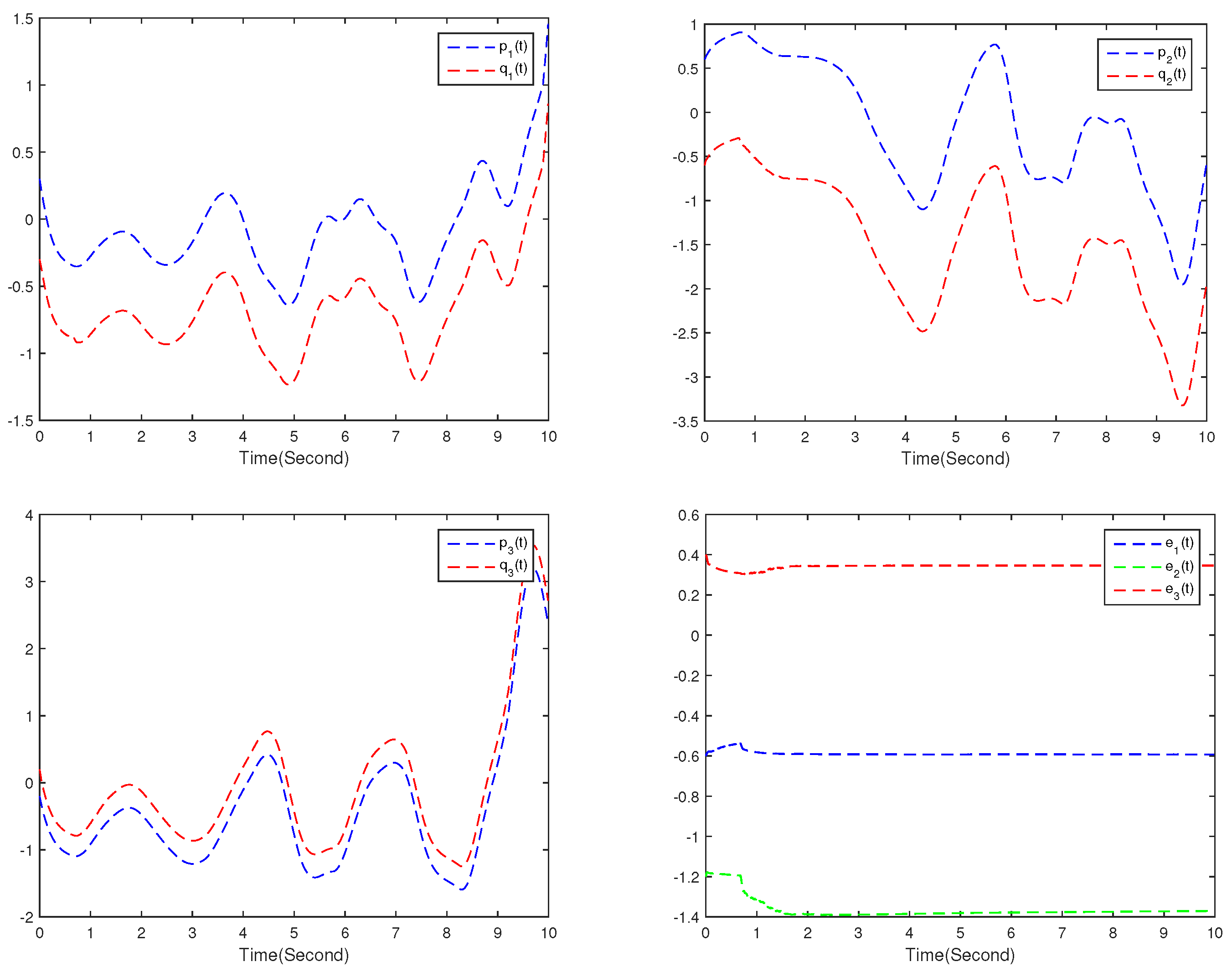
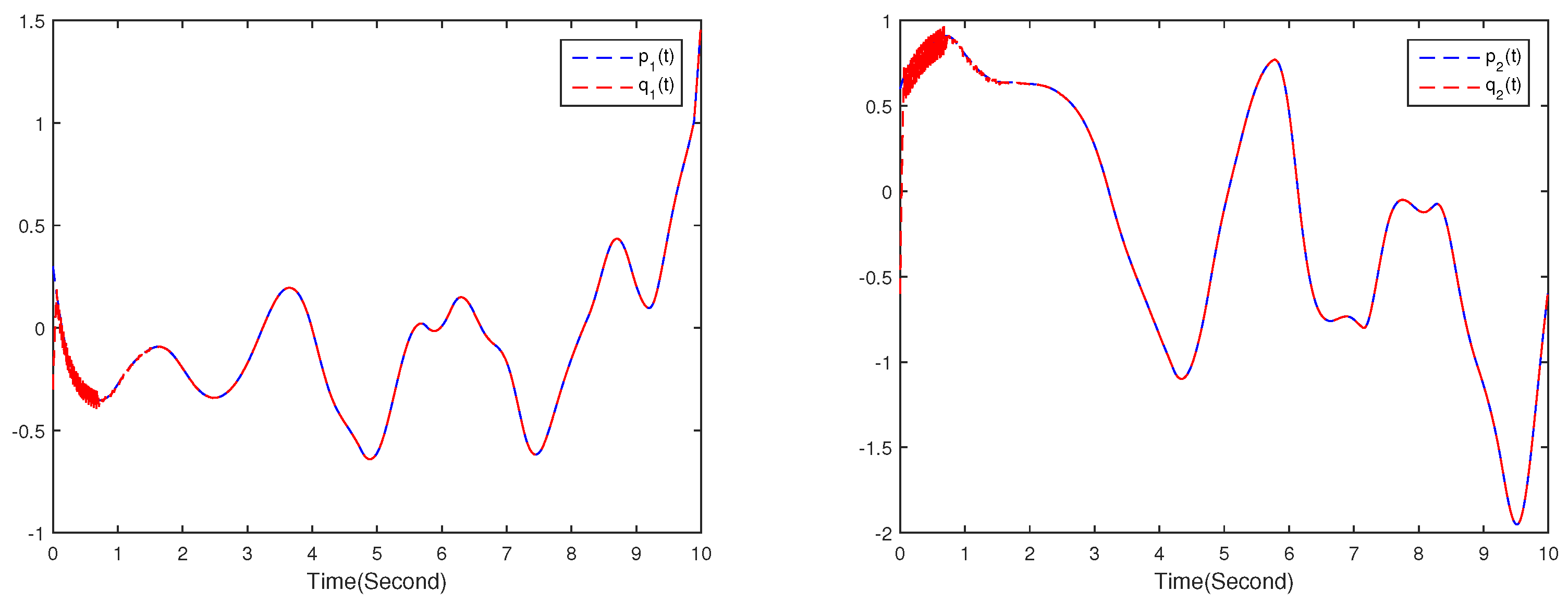
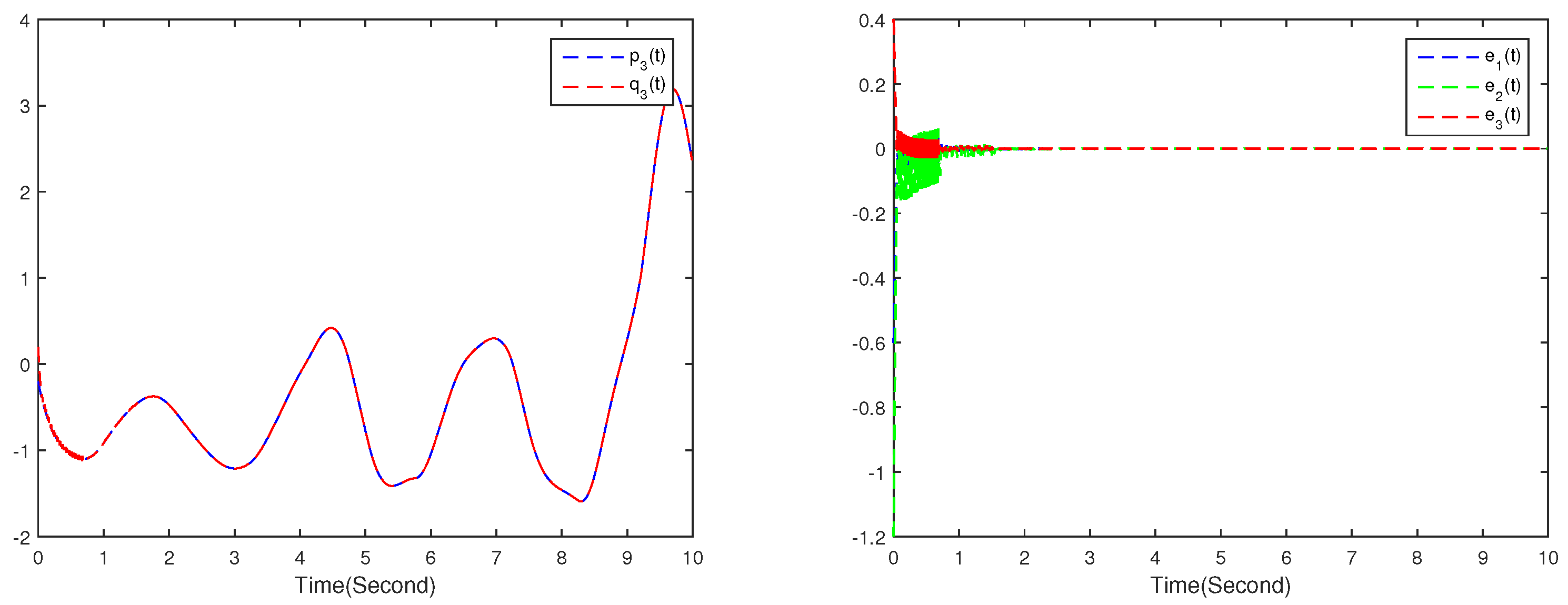
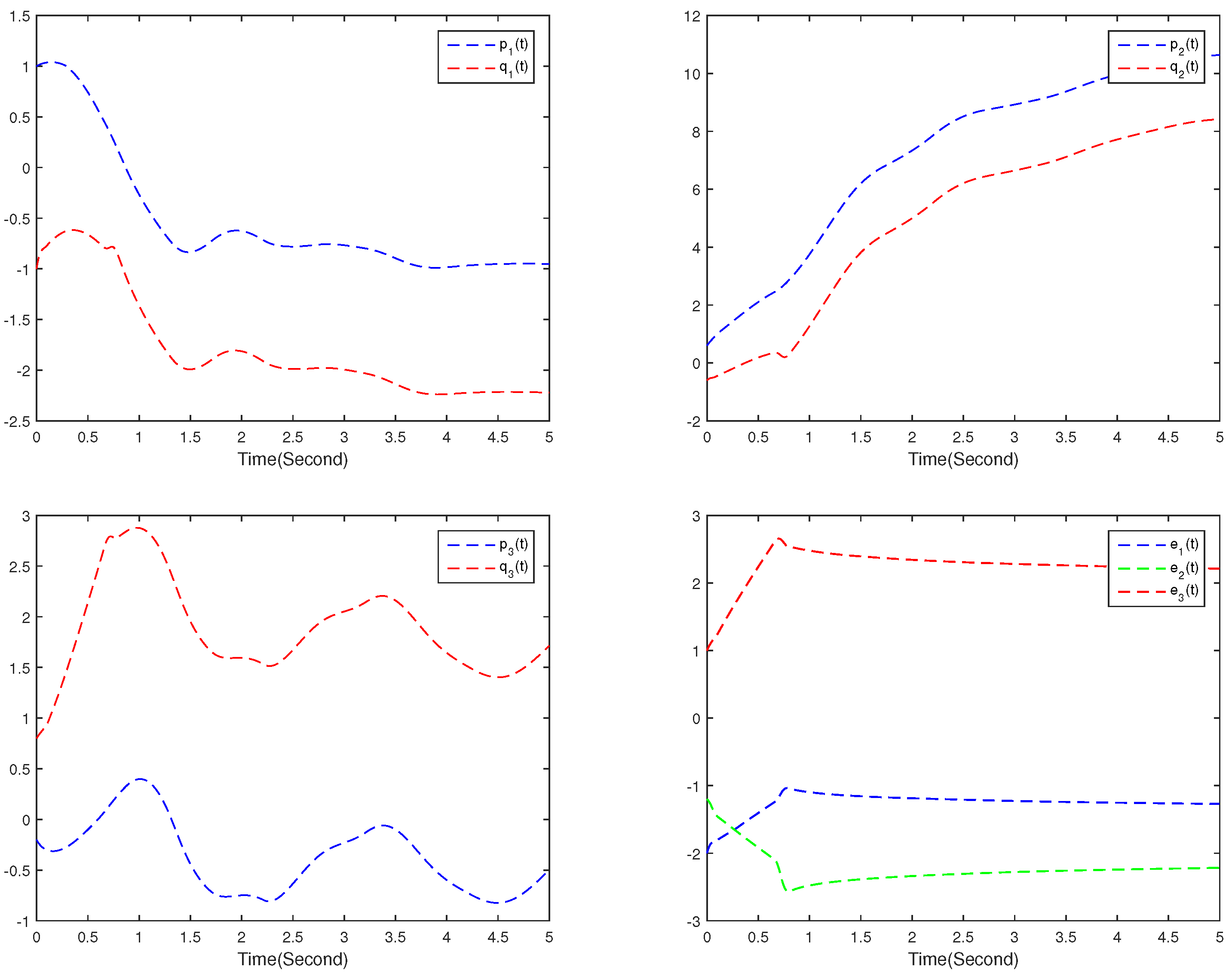
4. Numerical Simulations

This section validates the effectiveness of Theorems 1 and 2 through two numerical examples.

Example 1. 

Take the drive–response systems

$$\left\{\begin{array}{cc}\hfill {}_{t_0}{}^{C}D^{\omega }{p}_i\left(t\right)=& -{\alpha }_i{p}_i(t-{\tau }_1\left(t\right))+\sum _{r=1}^3{\varphi }_{ir}\left(p_i\left(t\right)\right)f_r\left(p_r\left(t\right)\right)\hfill \\ \hfill & +\sum _{r=1}^3{\psi }_{ir}\left(p_i(t-{\tau }_2\left(t\right))\right)f_r\left(p_r(t-{\tau }_2\left(t\right))\right)+H_i\left(p\left(t\right)\right)+I_i\hfill \\ \hfill p_i\left(\upsilon \right)=& {\zeta }_i\left(\upsilon \right),\upsilon \in [-\tau ,t_0],i=1,2,3,\hfill \end{array}\right.$$

(27)

where

$$\begin{array}{cc}\hfill H_i\left(p\left(t\right)\right)=& \sum _{r=1}^3{g}_{ir}{v}_r+\underset{r=1}{\overset{3}{\bigwedge }}{T}_{ir}{\nu }_r+\underset{r=1}{\overset{3}{\bigwedge }}{a}_{ir}{f}_r\left(p_r(t-{\tau }_2\left(t\right))\right)+\underset{r=1}{\overset{3}{\bigvee }}{S}_{ir}{\nu }_r\hfill \\ \hfill & +\underset{r=1}{\overset{3}{\bigvee }}{b}_{ir}{f}_r\left(p_r(t-{\tau }_2\left(t\right))\right)\hfill \end{array}$$

with following system parameters:

$$\left\{\begin{array}{cc}\hfill {\Gamma }_1& ={\Gamma }_2={\Gamma }_3=1,{\alpha }_1={\alpha }_2={\alpha }_3=1,l=1.8,\omega =0.95\hfill \\ \hfill {\varphi }_{11}^{\prime }& =2.0,{\varphi }_{12}^{\prime }=-1,{\varphi }_{13}^{\prime }=1.8,{\varphi }_{21}^{\prime }=0.8,{\varphi }_{22}^{\prime }=1.5,{\varphi }_{23}^{\prime }=-1.0,\hfill \\ \hfill {\varphi }_{31}^{\prime }& =-1.1,{\varphi }_{32}^{\prime }=2.0,{\varphi }_{33}^{\prime }=1.5,{\varphi }_{11}^{″}=2.2,{\varphi }_{12}^{″}=-1.2,{\varphi }_{13}^{″}=2.0,\hfill \\ \hfill {\varphi }_{21}^{″}& =1.0,{\varphi }_{22}^{″}=1.8,{\varphi }_{23}^{″}=-1.5,{\varphi }_{31}^{″}=-1.0,{\varphi }_{32}^{″}=1.7,{\varphi }_{33}^{″}=2.0\hfill \\ \hfill {\psi }_{11}^{\prime }& =-2.0,{\psi }_{12}^{\prime }=-0.5,{\psi }_{13}^{\prime }=1.5,{\psi }_{21}^{\prime }=2.5,{\psi }_{22}^{\prime }=5.0,{\psi }_{23}^{\prime }=-2.5\hfill \\ \hfill {\psi }_{31}^{\prime }& =2.4,{\psi }_{32}^{\prime }=-2.0,{\psi }_{33}^{\prime }=4.5,{\psi }_{11}^{″}=-1.5,{\psi }_{12}^{″}=-1.0,{\psi }_{13}^{″}=2.0\hfill \\ \hfill {\psi }_{21}^{″}& =2.2,{\psi }_{22}^{″}=4.5,{\psi }_{23}^{″}=-3.0,{\psi }_{31}^{″}=2.0,{\psi }_{32}^{″}=-18,{\psi }_{33}^{″}=5\hfill \\ \hfill a_{11}& =a_{13}=a_{22}=a_{23}=a_{31}=a_{32}=0.1,a_{12}=a_{21}=-0.2,a_{33}=-0.1\hfill \\ \hfill b_{11}& =b_{13}=b_{22}=b_{31}=0.2,b_{12}=b_{21}=-0.2,b_{23}=b_{32}=0.1,b_{33}=-0.1\hfill \\ \hfill S_{11}& =S_{22}=S_{33}=-0.1,S_{12}=S_{13}=S21=S_{23}=S_{31}=S_{32}=0.1\hfill \\ \hfill T_{11}& =T_{22}=T_{33}=-0.1,T_{12}=T_{13}=T_{21}=T_{23}=T_{31}=T_{32}=0.1\hfill \\ \hfill g_{ir}& =-1.0,v_r=-1,i,r=1,2.3\hfill \end{array}\right.$$

(28)

Let $f_i\left(p\left(t\right)\right)=tanh(|p\left(t\right)|)-1$, $I_i=0.1$, $L_i=1,i=1,2,3$, ${\tau }_1\left(t\right)=tanh\left(t\right)$, and ${\tau }_2\left(t\right)={\displaystyle \frac{e^t}{1+e^t}}$. The initial values of System (27) are ${\zeta }_1\left(\upsilon \right)=0.3,{\zeta }_2\left(\upsilon \right)=0.6,{\zeta }_3\left(\upsilon \right)=-0.2,\upsilon \in [-\tau \left(t\right),0]$.

The response system is

$$\left\{\begin{array}{cc}\hfill {}_{t_0}{}^{C}D^{\omega }{q}_i\left(t\right)=& -{\alpha }_i{q}_i(t-{\tau }_1\left(t\right))+\sum _{r=1}^3{\varphi }_{ir}\left(q_i\left(t\right)\right)f_r\left(q_r\left(t\right)\right)\hfill \\ \hfill +& \sum _{r=1}^3{\psi }_{ir}\left(q_i(t-{\tau }_2\left(t\right))\right)f_r\left(q_r(t-{\tau }_2\left(t\right))\right)+H_i\left(q\left(t\right)\right)+u_i+I_i\hfill \\ \hfill q_i\left(\upsilon \right)=& {\xi }_i\left(\upsilon \right),\upsilon \in [-\tau ,t_0],i=1,2,3,\hfill \end{array}\right.$$

(29)

where

$$\begin{array}{cc}\hfill H_i\left(q\left(t\right)\right)=& \sum _{r=1}^3{g}_{ir}{v}_r+\underset{r=1}{\overset{3}{\bigwedge }}{T}_{ir}{\nu }_r+\underset{r=1}{\overset{3}{\bigwedge }}{a}_{ir}{f}_r\left(q_r(t-{\tau }_2\left(t\right))\right)+\underset{r=1}{\overset{3}{\bigvee }}{S}_{ir}{\nu }_r\hfill \\ \hfill & +\underset{r=1}{\overset{3}{\bigvee }}{b}_{ir}{f}_r\left(q_r(t-{\tau }_2\left(t\right))\right)\hfill \end{array}$$

The parameters are the same as those in System (27). The initial values of System (29) are ${\xi }_1\left(\upsilon \right)=-0.3,{\xi }_2\left(\upsilon \right)=-0.6,{\xi }_3\left(\upsilon \right)=0.2,\upsilon \in [-\tau \left(t\right),0]$.

According to Theorem 1, the control parameters ${\theta }_i,{\delta }_i,{\eta }_i,i=1,2,3$ should satisfy

$$\left\{\begin{array}{cc}\hfill {\theta }_i& \ge {\alpha }_i\hfill \\ \hfill {\delta }_i& \ge {\displaystyle \frac{L_i}{{\lambda }_i}}\sum _{r=1}^3{\lambda }_r|{\varphi }_{ri}|\hfill \\ \hfill {\eta }_i& \ge {\displaystyle \frac{L_i}{{\lambda }_i}}\sum _{r=1}^3{\lambda }_r\left(|{\psi }_{ri}|+|a_{ri}|+|b_{ri}|\right)\hfill \end{array}\right.$$

Here, we choose

$$\left\{\begin{array}{cc}\hfill {\eta }_1& =5.5,{\eta }_2=6.2,{\eta }_3=6.7,\hfill \\ \hfill {\theta }_1& ={\theta }_2={\theta }_3=1.0,\hfill \\ \hfill {\delta }_1& ={\delta }_2={\delta }_3=10.7\hfill \\ \hfill {\gamma }_1& ={\gamma }_2={\gamma }_3=4\hfill \\ \hfill {\sigma }_1& ={\sigma }_2={\sigma }_3=0.01\hfill \\ \hfill {\lambda }_1& ={\lambda }_2={\lambda }_3=1.0\hfill \end{array}\right.$$

(30)

Figure 1 and Figure 2 present the state trajectories of Systems (27) and (29) with and without a controller. No synchronization can be achieved without a controller. But, synchronization is achieved within a finite time with a controller (5). In addition, according to Theorem 1, $T_{max}=1.6874$ can be computed using Formula (8). Therefore, Theorem 1 is effective.

Example 2. 

For System (27), the system’s parameter selection is as follows:

$$\left\{\begin{array}{cc}\hfill {\Gamma }_1& ={\Gamma }_2={\Gamma }_3=1,{\alpha }_1={\alpha }_2={\alpha }_3=1,l=1.8,\omega =0.9\hfill \\ \hfill {\varphi }_{11}^{\prime }& =2.0,{\varphi }_{12}^{\prime }=-1.1,{\varphi }_{13}^{\prime }=2.1,{\varphi }_{21}^{\prime }=1.1,{\varphi }_{22}^{\prime }=1.8,{\varphi }_{23}^{\prime }=-1.3,\hfill \\ \hfill {\varphi }_{31}^{\prime }& =-1.2,{\varphi }_{32}^{\prime }=1.7,{\varphi }_{33}^{\prime }=2.1,{\varphi }_{11}^{″}=2.1,{\varphi }_{12}^{″}=-1.0,{\varphi }_{13}^{″}=1.8,\hfill \\ \hfill {\varphi }_{21}^{″}& =0.8,{\varphi }_{22}^{″}=1.5,{\varphi }_{23}^{″}=-1.0,{\varphi }_{31}^{″}=-1.1,{\varphi }_{32}^{″}=2.1,{\varphi }_{33}^{″}=1.5\hfill \\ \hfill {\psi }_{11}^{\prime }& =-1.8,{\psi }_{12}^{\prime }=-1.1,{\psi }_{13}^{\prime }=2.1,{\psi }_{21}^{\prime }=2.2,{\psi }_{22}^{\prime }=4.5,{\psi }_{23}^{\prime }=-3.1\hfill \\ \hfill {\psi }_{31}^{\prime }& =2.1,{\psi }_{32}^{\prime }=-1.8,{\psi }_{33}^{\prime }=5.1,{\psi }_{11}^{″}=-2.1,{\psi }_{12}^{″}=-0.5,{\psi }_{13}^{″}=1.8\hfill \\ \hfill {\psi }_{21}^{″}& =2.5,{\psi }_{22}^{″}=5.1,{\psi }_{23}^{″}=-2.5,{\psi }_{31}^{″}=2.4,{\psi }_{32}^{″}=-2.1,{\psi }_{33}^{″}=4.5\hfill \\ \hfill a_{11}& =a_{13}=a_{22}=a_{23}=a_{31}=a_{32}=0.1,a_{12}=a_{21}=-0.2,a_{33}=-0.1\hfill \\ \hfill b_{11}& =b_{13}=b_{22}=b_{31}=0.2,b_{12}=b_{21}=-0.2,b_{23}=b_{32}=0.1,b_{33}=-0.1\hfill \\ \hfill S_{ir}& =0.1,T_{ir}=0.1,g_{ir}=1.0,v_r=1.0,i,r=1,2.3\hfill \end{array}\right.$$

(31)

Let $f_i\left(p\left(t\right)\right)=tanh(|p\left(t\right)|)-1$, $I_i=0.1$, $L_i=1,i=1,2,3$. ${\tau }_1\left(t\right)=tanh\left(t\right)$, ${\tau }_2\left(t\right)={\displaystyle \frac{e^t}{1+e^t}}$. The initial values of System (27) are ${\zeta }_1\left(\upsilon \right)=1,{\zeta }_2\left(\upsilon \right)=0.6,{\zeta }_3\left(\upsilon \right)=-0.2,\upsilon \in [-\tau \left(t\right),0]$.

The parameters of Response System (29) are the same as those in System (27). The initial values of System (29) are ${\xi }_1\left(\upsilon \right)=-1,{\xi }_2\left(\upsilon \right)=-0.6,{\xi }_3\left(\upsilon \right)=0.8,\upsilon \in [-\tau \left(t\right),0]$.

According to Theorem 2, the control gains ${\widehat{\theta }}_i,{\widehat{\delta }}_i,{\widehat{\eta }}_i,i=1,2,3$ should satisfy

$$\left\{\begin{array}{cc}\hfill {\widehat{\theta }}_i& \ge {\alpha }_i\hfill \\ \hfill {\widehat{\delta }}_i& \ge {\displaystyle \frac{L_i}{{\lambda }_i}}\sum _{r=1}^M{\lambda }_r|{\varphi }_{ri}|\hfill \\ \hfill {\widehat{\eta }}_i& \ge {\displaystyle \frac{L_i}{{\lambda }_i}}\sum _{r=1}^M{\lambda }_r\left(|{\psi }_{ri}|+|a_{ri}|+|b_{ri}|\right)\hfill \end{array}\right.$$

Here, we choose

$$\left\{\begin{array}{cc}\hfill {\widehat{\theta }}_1& =1.0,{\widehat{\theta }}_2=2.0,{\widehat{\theta }}_3=3.0,\hfill \\ \hfill {\widehat{\delta }}_1& =4.4,{\widehat{\delta }}_2=6.0,{\widehat{\delta }}_3=6.5,\hfill \\ \hfill {\widehat{\eta }}_1& =8.0,{\widehat{\eta }}_2=9.2,{\widehat{\eta }}_3=11.0,\hfill \\ \hfill {\gamma }_1& ={\gamma }_2={\gamma }_3=2,{\sigma }_1={\sigma }_2={\sigma }_3=0.1\hfill \\ \hfill {\lambda }_1& ={\lambda }_2={\lambda }_3=1.0,{\kappa }_1={\kappa }_2={\kappa }_3=1,\hfill \\ \hfill {\rho }_1& ={\rho }_2={\rho }_3=3,{\varrho }_1={\varrho }_2={\varrho }_3=2,\hfill \\ \hfill {ϵ}_1& =3,{ϵ}_2=4,{ϵ}_3=5.\hfill \end{array}\right.$$

(32)

Let ${\widehat{\theta }}_i\left(0\right)=1,{\widehat{\delta }}_i\left(0\right)=1,{\widehat{\eta }}_i\left(0\right)=1,$ and $i=1,2,3$,

Figure 3 and Figure 4 depict the state trajectories of Systems (27) and (29) with and without a controller. No synchronization can be achieved without a controller. But, synchronization is achieved within a finite time with a controller (6). In addition, according to Theorem 2, $T_{max}=0.8913$ when using Formula (21). As shown in Figure 5 and Figure 6, the adaptive control gains ${\kappa }_i\left(t\right)$ and ${\theta }_{ir}\left(t\right)$, $(i,r=1,2,3)$ converge to certain values within a finite time. Therefore, Theorem 2 is effective.

5. Conclusions

In this paper, the FTS and AFTS of FOMFNNs with leakage and transmission delays were investigated. Under a Filippov-like fractional-order differential inclusions theory and set-valued map, applying the Lyapunov functional method and the fractional-order differential inequalities allowed us to establish several new and useful criteria to achieve FTS and AFTS for FOMFNNs with leakage and transmission delays. In addition, the settling time is also presented. Finally, two numerical examples and their simulations are provided to demonstrate the validity of the obtained results. Future works will focus on the study of the described performance synchronization control for FOMFNNs with leakage and transmission delays.

References

1. Struko, D.; Snider, G.; Stewart, D. The missing memristor found. Nature 2008, 453, 80–83. [Google Scholar] [CrossRef] [PubMed]
2. Yao, P.; Wu, H.; Gao, B.; Tang, J.; Zhang, Q.; Zhang, W.; Yang, J.J.; Qian, H. Fully hardware-implemented memristor convolutional neural network. Nature 2020, 577, 641–646. [Google Scholar] [CrossRef] [PubMed]
3. Chen, J.; Zeng, Z.; Jiang, P. Global Mittag-Leffler stability and synchronization of memristor-based fractional-order neural networks. Neural Netw. 2014, 51, 1–8. [Google Scholar] [CrossRef] [PubMed]
4. Zhang, J.; Lu, J.; Jin, X.; Yang, X.Y. Novel results on asymptotic stability and synchronization of fractional-order memristive neural networks with time delays: The 0 < δ ≤ 1 case. Neural Netw. 2023, 167, 680–691. [Google Scholar]
5. Yao, X.; Liu, X.; Zhong, S. Exponential stability and synchronization of Memristor-based fractional-order fuzzy cellular neural networks with multiple delays. Neurocomputing 2021, 419, 239–250. [Google Scholar] [CrossRef]
6. Ding, Z.; Chen, C.; Wen, S.; Li, S.; Wang, L. Lag projective synchronization of nonidentical fractional delayed memristive neural networks. Neurocomputing 2022, 469, 138–150. [Google Scholar] [CrossRef]
7. Li, H.; Cao, J.; Hu, C.; Zhang, L.; Jiang, H. Adaptive control-based synchronization of discrete-time fractional-order fuzzy neural networks with time-varying delays. Neural Netw. 2023, 168, 59–73. [Google Scholar] [CrossRef]
8. Zhang, L.; Yang, Y. Finite time impulsive synchronization of fractional order memristive BAM neural networks. Neurocomputing 2020, 384, 213–224. [Google Scholar] [CrossRef]
9. Du, F.; Lu, J. New criterion for finite-time synchronization of fractional order memristor-based neural networks with time delay. Appl. Math. Comput. 2021, 389, 125616. [Google Scholar] [CrossRef]
10. Anbalagan, P.; Ramachandran, R.; Alzabut, J.; Hincal, E.; Niezabitowski, M. Improved results on finite-time passivity and synchronization problem for fractional-order memristor-based competitive neural networks: Interval matrix approach. Fractal Fract. 2022, 6, 36. [Google Scholar] [CrossRef]
11. Sun, Y.; Liu, Y.; Liu, L. Asymptotic and finite-time synchronization of fractional-order memristor-based inertial neural networks with time-varying delay. Fractal Fract. 2022, 6, 350. [Google Scholar] [CrossRef]
12. Wei, R.; Cao, J.; Alsaedi, A. Fixed-time synchronization of memristive Cohen-Grossberg neural networks with impulsive effects. Int. J. Control Autom. Syst. 2018, 16, 2214–2224. [Google Scholar] [CrossRef]
13. Ren, H.; Peng, Z.; Gu, Y. Fixed-time synchronization of stochastic memristor-based neural networks with adaptive control. Neural Netw. 2020, 130, 165–175. [Google Scholar] [CrossRef] [PubMed]
14. Zhao, Y.; Ren, S.; Kurths, J. Finite-time and fixed-time synchronization for a class of memristor-based competitive neural networks with different time scales. Chaos Solitons Fractals 2021, 148, 111033. [Google Scholar] [CrossRef]
15. Wei, R.; Cao, J.; Gorbachev, S. Fixed-time control for memristor-based quaternion-valued neural networks with discontinuous activation functions. Cogn. Comput. 2023, 15, 50–60. [Google Scholar] [CrossRef]
16. Jia, T.; Chen, X.; Yao, X.; Zhao, F.; Qiu, J. Adaptive fixed-time synchronization of delayed memristor-based neural networks with discontinuous activations. CMES-Comput. Model. Eng. Sci. 2023, 134, 221–239. [Google Scholar] [CrossRef]
17. Sun, Y.; Liu, Y.; Liu, L. Fixed-time synchronization for fractional-order cellular inertial fuzzy neural networks with mixed time-varying delays. Fractal Fract. 2024, 8, 97. [Google Scholar] [CrossRef]
18. Zhao, F.; Jian, J.; Wang, B. Finite-time synchronization of fractional-order delayed memristive fuzzy neural networks. Fuzzy Sets Syst. 2023, 467, 108578. [Google Scholar] [CrossRef]
19. Du, F.; Lu, J. Adaptive finite-time synchronization of fractional-order delayed fuzzy cellular neural networks. Fuzzy Sets Syst. 2023, 466, 108480. [Google Scholar] [CrossRef]
20. Jian, J.; Duan, L. Finite-time synchronization for fuzzy neutral-type inertial neural networks with time-varying coefficients and proportional delays. Fuzzy Sets Syst. 2020, 381, 51–67. [Google Scholar] [CrossRef]
21. Gopalsamy, K. Leakage delays in BAM. J. Math. Anal. Appl. 2007, 325, 1117–1132. [Google Scholar] [CrossRef]
22. Alia, M.; Narayanana, G.; Sarohab, S.; Priya, B.; Thakur, G.K. Finite-time stability analysis of fractional-order memristive fuzzy cellular neural networks with time delay and leakage term. Math. Comput. Simul. 2021, 185, 468–485. [Google Scholar]
23. Yan, H.; Qiao, Y.; Duan, L.; Miao, J. New results of quasi-projective synchronization for fractional-order complex-valued neural networks with leakage and discrete delays. Chaos Solitons Fractals 2022, 159, 112121. [Google Scholar] [CrossRef]
24. Zhu, M.; Wang, B.; Wu, Y. Stability and Hopf bifurcation for a quaternion-valued three-neuron neural network with leakage delay and communication delay. J. Frankl. Inst. 2023, 360, 12969–12989. [Google Scholar] [CrossRef]
25. Yuan, S.; Wang, Y.; Zhang, X. Global exponential synchronization of switching neural networks with leakage time-varying delays. Commun. Nonlinear Sci. Numer. Simul. 2024, 133, 107979. [Google Scholar] [CrossRef]
26. Zhang, H.; Cheng, J.; Zhang, H.; Zhang, W.; Cao, J. Quasi-uniform synchronization of Caputo type fractional neural networks with leakage and discrete delays. Chaos Solitons Fractals 2021, 152, 11432. [Google Scholar] [CrossRef]
27. Kao, Y.; Li, Y.; Park, J.; Chen, X. Mittag-Leffler synchronization of delayed fractional memristor neural networks via adaptive control. IEEE Trans. Neural Netw. Learn. Syst. 2021, 32, 2279–2284. [Google Scholar] [CrossRef] [PubMed]
28. Yang, S.; Yu, J.; Hu, C.; Jiang, H. Finite-time synchronization of memristive neural networks with fractional-order. IEEE Trans. Syst. Man Cybern. Syst. 2021, 51, 3739–3750. [Google Scholar] [CrossRef]
29. Filippov, A. Differential Equations with Discontinuous Righthand Sides; Kluwer Academic Publishers: Boston, MA, USA, 1988. [Google Scholar]
30. Li, C.; Deng, W. Remarks on fractional derivatives. Aied Math. Comput. 2007, 187, 777–784. [Google Scholar] [CrossRef]
31. Zhang, S.; Yu, Y.; Wang, H. Mittag-Leffler stability of fractional-order hopfield neural networks. Nonlinear Anal. Hybrid Syst. 2015, 16, 104–121. [Google Scholar] [CrossRef]
32. Zheng, M.; Li, L.; Peng, H.; Xiao, J.; Yang, Y.; Zhang, Y.; Zhao, H. Fixed-time synchronization of memristor-based fuzzy cellular neural network with time-varying delay. J. Frankl. Inst. 2018, 355, 6780–6809. [Google Scholar] [CrossRef]
33. Sun, Y.; Liu, Y. Fixed-time synchronization of delayed fractional-order memristor-based fuzzy cellular neural networks. IEEE Access 2020, 8, 165951–165962. [Google Scholar] [CrossRef]
Figure 1. State trajectories of p i ( t ) , q i ( t ) , and e i ( t ) without controller.
Fractalfract 09 00241 g001
Figure 2. State trajectories of p i ( t ) , q i ( t ) , and e i ( t ) with controller.
Fractalfract 09 00241 g002aFractalfract 09 00241 g002b
Figure 3. State trajectories of p i ( t ) , q i ( t ) , and e i ( t ) without controller.
Fractalfract 09 00241 g003
Figure 4. State trajectories of p i ( t ) , q i ( t ) , and e i ( t ) with controller.
Fractalfract 09 00241 g004
Figure 5. State trajectories of control gains δ i ( t ) , i = 1 , 2 , 3 .
Fractalfract 09 00241 g005
Figure 6. State trajectories of control gains θ i ( t ) and η i ( t ) , i = 1 , 2 , 3 .
Fractalfract 09 00241 g006
Disclaimer/Publisher’s Note: The statements, opinions and data contained in all publications are solely those of the individual author(s) and contributor(s) and not of MDPI and/or the editor(s). MDPI and/or the editor(s) disclaim responsibility for any injury to people or property resulting from any ideas, methods, instructions or products referred to in the content.