Static Shift Correction and Fractal Characteristic Analysis of Time-Frequency Electromagnetic Data

Abstract

The static shift effect is a distortion in electromagnetic data that severely impacts exploration results. Traditional static effect correction methods are often ineffective, prone to overcorrection or undercorrection, and make it difficult to accurately assess the applicability of the correction. Furthermore, some correction processes require additional data, which increases correction costs. This paper first presents the theoretical foundation for correcting static shift effects in the electric field components using magnetic field component information. Based on time-frequency electromagnetic exploration technology, a method is proposed to correct static shift effects in the electric field by using simultaneously collected magnetic field data, aiming to address the distortion issues caused by static shift effects in the electric field and apparent resistivity. The method is validated through both theoretical models and field data, demonstrating its excellent correction performance. Additionally, the paper introduces the use of the multifractal spectrum analysis algorithm to analyze profile measurement points and study the fractal dimension characteristics of static shift effects, providing an effective way to evaluate the appropriateness and potential overcorrection of the correction. Finally, the multifractal features of field data are discussed, validating the ability of the multifractal spectrum to identify subsurface electrical complexity.

1. Introduction

In electromagnetic exploration, the static shift effect is a phenomenon in which the presence of electrically heterogeneous bodies near the surface causes the accumulation of static charges on their surfaces due to the horizontal electric field, distorting the amplitude of the measured electric field and leading to a shift in apparent resistivity with logarithmic frequency, severely affecting the effectiveness of exploration [1,2,3,4,5].

To mitigate this effect, several methods have been developed, primarily falling into three categories: First, correction methods that incorporate prior information. For example, statistical variations in profile resistivity can be obtained through outcrop geology and resistivity measurements in the study area, or through statistical analysis of drilling data [1] and high-quality resistivity sounding curves [2,6,7,8]. However, such prior information is difficult to match perfectly with electromagnetic exploration areas and can be costly. Second, low-pass filtering methods. Since static shifts exhibit high-frequency characteristics, low-pass filtering can be applied to suppress such effects. The electromagnetic array profiling method, originally proposed by Bostick [6], uses spatial filtering for correction. Torres-Verdín and Bostick [9] analyzed the secondary magnetic field and electric field anomalies of shallow subsurface anomalies using the Born approximation method. However, spatial filtering methods are highly sensitive to the input parameters selected for the filter and heavily rely on the experience of data processors, often resulting in over- or under-correction, affecting exploration results. Third, correction using other data unaffected by static shifts. This involves using simultaneously collected electromagnetic data unaffected by static shifts, such as independently collected transient electromagnetic data [10,11,12,13], for correction, which has shown some effectiveness. Although this method avoids human interference, it requires independent acquisition systems, increasing workload and potentially being affected by survey point locations and acquisition parameters. Tournerie et al. [14] proposed a method to estimate apparent resistivity using the spatial distribution of phases, but this method requires at least 30 survey points and points not affected by static shift effects, making it unsuitable for independent or small-scale applications. To address these issues, this paper proposes a static shift correction method based on time-frequency electromagnetic (TFEM) data.

Time-frequency electromagnetic (TFEM) technology is a novel technique that combines time and frequency information for electromagnetic exploration [15,16]. Developed over more than two decades to meet the needs of oil and gas exploration transitioning from structural trap exploration to lithological and other hidden trap exploration, it has become a mature technology for oil and gas exploration and oil-bearing trap detection, widely applied with good exploration results [16,17,18,19,20]. TFEM technology simultaneously measures horizontal electric and vertical magnetic fields, leveraging the complementary advantages of electric and magnetic fields to enhance exploration effectiveness. However, current static shift correction methods in TFEM still use traditional filtering techniques, which may result in under- or overcorrection. To fully utilize the advantage of TFEM’s simultaneous acquisition of vertical magnetic and horizontal electric fields for efficient static-shift correction, this paper proposes a new static shift correction method. Additionally, traditional static shift correction methods lack quantitative standards to judge the suitability of correction. To solve this problem, we introduce fractal characteristic analysis.

Fractal characteristic analysis has been gradually applied to geophysical data analysis in recent years [21,22,23,24,25]. Multifractal analysis, which studies the global characteristics of a system from its local properties, mainly discusses the distribution laws of probabilities using statistical physics methods. Halsey et al. [26] proposed the mathematical framework for the multifractal spectrum, discussing the singularities of fractal measures and the mathematical foundation of multifractal analysis. We introduce this method to perform multifractal spectrum analysis on electric field data, analyzing the fractal dimension characteristics of static shift effects caused by shallow subsurface electrical heterogeneities, and further exploring the possibility of identifying geological anomaly features.

In this work, we first introduce the theoretical basis of static shift effects, followed by a description of the proposed correction method and the use of multifractal spectrum analysis. We then apply the method to both synthetic and field data to demonstrate its effectiveness and evaluate the corresponding fractal characteristics. Finally, we discuss the broader implications of the results and summarize the key findings.

2. Materials and Methods

2.1. Principle of Static Shift Effects

The secondary field response of the shallow surface anomaly $(x_0,y_0,z_0)$ in the far field case is used as an example to analyze the mechanism of the static shift effect. In electromagnetic exploration, the observed electromagnetic field can be written as the sum of the primary and secondary fields:

$$E=E_1+E_2$$

(1)

$$H=H_1+H_2$$

(2)

where $E_0$ and $H_0$ represent the primary field of the electric and magnetic fields, respectively, and $E_2$ represents the secondary field. Conductivity anomalies in the subsurface can be represented in a similar form:

$$\sigma ={\sigma }_0+\Delta \sigma$$

(3)

where the uniform earth conductivity is ${\sigma }_0$, and the difference between the anomaly and the background conductivity is $\Delta \sigma$.

Under far-field conditions, the relationship between the electromagnetic fields can be described by a system of Maxwell’s equations:

$$\nabla \times E=-i\omega \mu H$$

(4)

$$\nabla \times H=\sigma E$$

(5)

where i is the imaginary unit, $\omega$ is the angular frequency of an electromagnetic wave, and $\mu$ is the magnetic permeability in a vacuum.

The Helmholtz equation for the secondary electric field can be obtained by substituting Equations (1)–(3) into (4) and (5):

$${\nabla }^2{E}_2+i\omega \mu E_2=i\omega \mu \Delta \sigma E$$

(6)

If $\Delta \sigma <<\sigma$, the Helmholtz equations can be written in integral form with the help of Green’s function, using the first-order Born approximation and replacing the total field with a primary field:

$$E_2\left(\overrightarrow{r}\right)={\int }_v\Delta \sigma \left(r_0\right)G(r,r_0)E_1{e}^{-ik{z}_0}dv$$

(7)

The above equation can be written as follows:

$${\displaystyle \frac{{E_2}_j\left(\overrightarrow{r}\right)}{E_1}}={\int }_v{\rho }_n\left({\overrightarrow{r}}_0\right)K_{ej}(\overrightarrow{r},{\overrightarrow{r}}_0)dv$$

(8)

The kernel function of the MT electric field orthogonal problem is:

$$K_{ej}(\overrightarrow{r},{\overrightarrow{r}}_0)=-\Delta {\sigma }_0{G}_j(\overrightarrow{r},{\overrightarrow{r}}_0)E_1{e}^{-ik{z}_0}$$

(9)

If the coordinates of the surface receiving point are $(x_0,y_0,0)$, then it can be set as follows:

$$K_{ej}(\overrightarrow{r},{\overrightarrow{r}}_0)={\lambda }_{ej}(x_0-x,y_0-y,z_0)$$

(10)

In the Cartesian coordinate system, Equation (8) can be written as follows:

$${\displaystyle \frac{{E_2}_j\left(\overrightarrow{r}\right)}{E_1}}={\int }_0^{\infty }[{\lambda }_{ej}(x,y,z_0)\ast {\rho }_n(x,y,z_0)]d{z}_0$$

(11)

where * denotes a two-dimensional convolution about x and y. To obtain a more intuitive algebraic form, we perform a Fourier transform of the above equation to obtain the form in the wave number domain and set $\xi ,\eta ,\zeta$ to represent the wave number in the x-, y-, and z-directions, respectively.

$${\displaystyle \frac{E_j(\xi ,\eta )}{E_1}}={\int }_0^{\infty }[{\Lambda }_{ej}(\xi ,\eta ,z_0)\ast P(\xi ,\eta ,z_0)]d{z}_0$$

(12)

where $E_j(\xi ,\eta )$ denotes the Fourier transform of ${E_2}_j\left(\overrightarrow{r}\right)$, $\Lambda$ denotes the Fourier transform of $\lambda$, and $P(\xi ,\eta ,z_0)$ denotes the Fourier transform of ${\rho }_n(x,y,z_0)$. If $P(\xi ,\eta ,z_0)$ is regarded as the input and ${\displaystyle \frac{E_j(\xi ,\eta )}{E_0}}$ as the output, $\Lambda$ can be regarded as the transfer function of the linear system, and similarly, the linear integral equation of the quadratic magnetic field can be obtained in the wave number domain:

$${\displaystyle \frac{H_j(\xi ,\eta )}{H_0}}={\int }_0^{\infty }[{\Lambda }_{hj}(\xi ,\eta ,z_0)\ast P(\xi ,\eta ,z_0)]d{z}_0$$

(13)

The derivation process is omitted, and the electric-field Ex component transfer function is given directly:

$${\Lambda }_{ex}(\xi ,\eta )={\displaystyle \frac{i\omega \mu {\sigma }_0}{i\zeta }}{r}_1(\xi ,\eta )e^{-i(k+\zeta )z_0}+{\displaystyle \frac{{\xi }^2}{i\zeta }}{e}^{-i+\left(k\zeta \right)z_0}$$

(14)

The magnetic field $H_z$ component kernel function is:

$${\Lambda }_{hz}(\xi ,\eta )=-\sqrt{i\omega \mu {\sigma }_0}{r}_2(\xi ,\eta )e^{-i(k+\zeta )z_0}$$

(15)

where $r_1$, $r_2$ are parameters related to the wave number. Observation of the above equation shows that the electric field transfer function has two terms. The first term, which is frequency dependent, is referred to as the dynamic term and the second term, which is frequency independent, is the static term. For the anomaly with fixed depth $z_0$, the dynamic term for the data in the frequency domain varies with frequency $\omega$, while the static term is the same for different frequency data, and the static term is the reason for the static shift effect. And Equation (15) shows that there is no static term in the vertical component of the magnetic field, only a dynamic term. Thus, the magnetic field does not produce static shift effects.

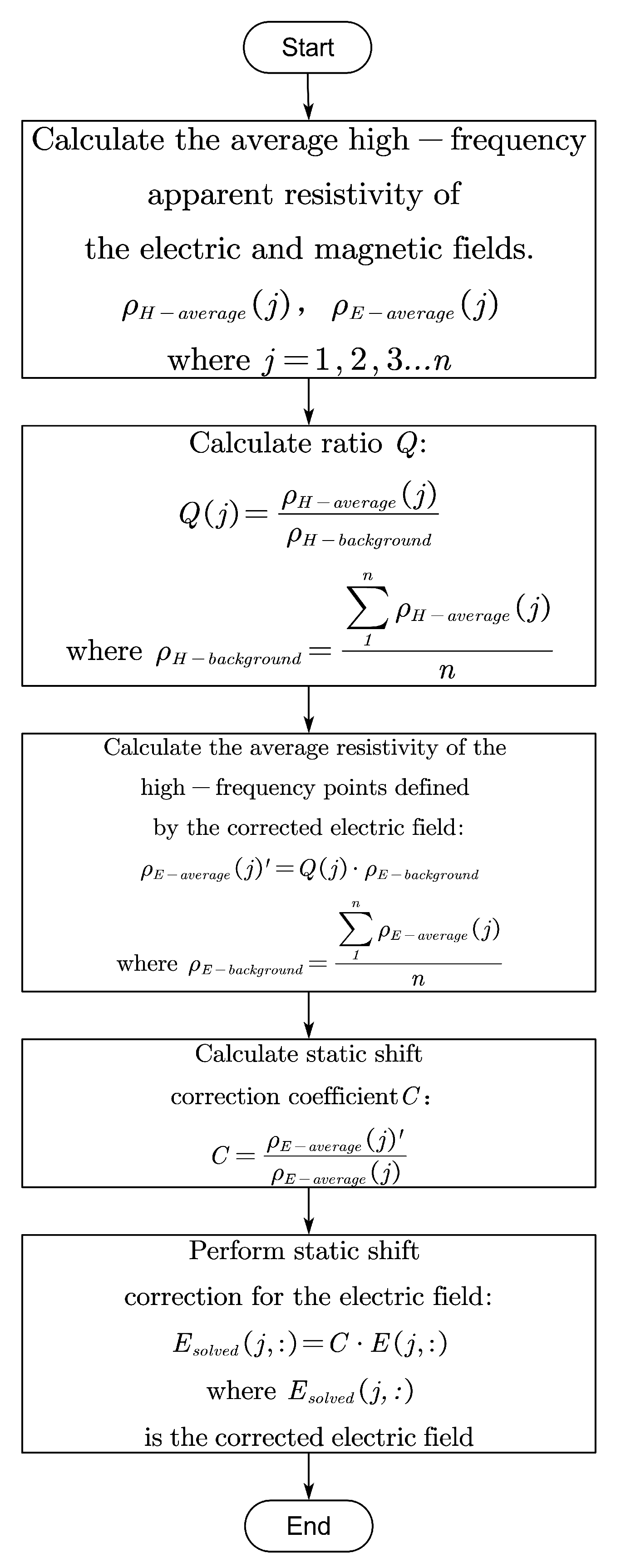
2.2. Time-Frequency Electromagnetic Static Shift Correction Method

Using the fact that the magnetic field or magnetic flux density components are not affected by the static shift effect, the electric field is corrected using apparent resistivity as an intermediary. The correction factor is initially derived by averaging the first three (or five) apparent resistivity values of the early magnetic field and the high-frequency electric field, respectively. This correction factor is then applied to the full frequency-domain data. Assuming a total of n measurement points, the specific method is outlined in Figure 1.

2.3. Multifractal Analysis of Electromagnetic Anomalies

Based on the theoretical analysis of static shift generation, it is evident that near-surface inhomogeneous conductivity bodies have different effects on the electric and magnetic fields. Therefore, we introduce the multifractal analysis method to distinguish the electric and magnetic field anomaly characteristics caused by near-surface inhomogeneous conductivity bodies.

Multifractals, also known as multiscale fractals, represent an advanced development of fractal theory in physics. The multifractal approach studies the overall characteristics of a system by examining its local features. Statistical physics methods are utilized primarily to discuss the distribution patterns of probability. The idea behind multifractal singularity spectrum analysis is to characterize the singularity properties of the normalized measure (distribution) defined on a fractal set to express its scaling behavior. The singularity of the distribution is represented by the singularity strength $\alpha$ and the corresponding distribution density $f\left(\alpha \right)$. The multifractal spectrum is then determined by the range of values of $\alpha$ and the function $f\left(\alpha \right)$. In order to calculate the multifractal singularity spectrum of electromagnetic field data, the box-counting method [26] is used in this paper:

For any given set of 1D electromagnetic field data, denoted as X, we divide it into several boxes with a scale $\epsilon$, covering the data. The probability measure of the normalized number of boxes $P_i\left(\epsilon \right)$ is then spatially defined.

$$P_i\left(\epsilon \right)={\displaystyle \frac{N_i\left(\epsilon \right)}{N}}$$

(16)

where $N_i$ is the electromagnetic field data (mass, number of points) in the i-th box, and N is the total sum of the 1D electromagnetic field data (mass, number of points). As in $\epsilon \to 0$, it can be assumed that the data are uniformly distributed across the boxes. For multifractal measures, for the i-th box on scale $\epsilon$, $P_i$ follows the following proportional relationship:

$$p_i\left(\epsilon \right)\sim {\epsilon }^{{\alpha }_i}$$

(17)

$$N_{\alpha }\left(\epsilon \right)\sim {\epsilon }^{f\left(\alpha \right)}$$

(18)

where ${\alpha }_i$ is the singularity scaling exponent and a partition function is defined as follows:

$$Z_q\left(\epsilon \right)=\sum _i^{n_i\left(\epsilon \right)}{P}_i^q$$

(19)

where $n_i\left(\epsilon \right)$ is the number of boxes on the scale $\epsilon$, and q is referred to as the weight factor. Its value can be arbitrary, but when $\left|q\right|$ reaches a certain level, further increases will no longer affect the multifractal spectrum.

Mass index:

$$\tau q=\underset{\epsilon \to 0}{lim}{\displaystyle \frac{log{Z}_q\left(\epsilon \right)}{log\epsilon }}$$

(20)

According to the Legendre transform, we can derive the multifractal singularity spectrum relationship for the electromagnetic field data:

$$f\left({\alpha }_q\right)=q{\alpha }_q-{\tau }_q$$

(21)

$${\alpha }_q={\displaystyle \frac{d{\tau }_q}{dq}}$$

(22)

Taking ${\alpha }_q$ as the horizontal coordinate and $f\left({\alpha }_q\right)$ as the vertical coordinate, the multifractal spectrum of the data from the electromagnetic field in 1D X can be obtained. The width of the multifractal spectrum, denoted as $\Delta \alpha$, is referred to as the inhomogeneity index:

$$\Delta \alpha ={\alpha }_{\max }-{\alpha }_{min}$$

(23)

For continuous and differentiable electromagnetic field data, $\Delta \alpha$ is a quantitative measure of the total rate of change (gradient) of all data points in the entire dataset. Data that are not differentiable, such as apparent resistivity variations in electromagnetic methods, serve as the overall quantitative indicator of the data’s inhomogeneity.

The width of the distribution density, denoted $f\left(\alpha \right)$, is referred to as the roughness index:

$$\Delta f\left(\alpha \right)={f\left(\alpha \right)}_{\max }-{f\left(\alpha \right)}_{\min }$$

(24)

where $\Delta f\left(\alpha \right)$ represents the difference in the distribution density extrema of all data points within the entire electromagnetic field data. The smoother and more uniform the data, the smaller the roughness index.

The inhomogeneity index $\Delta \alpha$ and the roughness index $\Delta f\left(\alpha \right)$ are two key parameters that describe the multifractal characteristics of the data. When the electromagnetic field data do not exhibit multifractal characteristics, both $\Delta \alpha$ and $\Delta f\left(\alpha \right)$ are zero. The more pronounced the multifractal characteristics of the data, the larger the values of $\Delta \alpha$ and $\Delta f\left(\alpha \right)$.

3. Results

3.1. Example of Static Shift Correction in a Theoretical Model

We design the 2.5D subsurface anomaly model Figure 2a and calculate its electromagnetic response Figure 2c, and as a control, we first calculate the electromagnetic response of anomalies without a shallow surface Figure 2b and compare it with the results of the processing using this algorithm Figure 2d.

It can be observed that the current algorithm effectively suppresses static shift, and the results closely match the theoretical results without static shift effects.

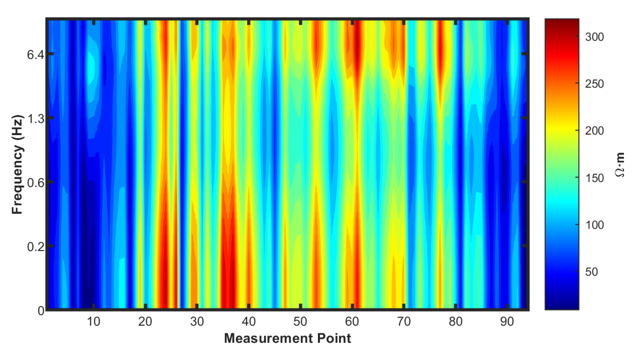
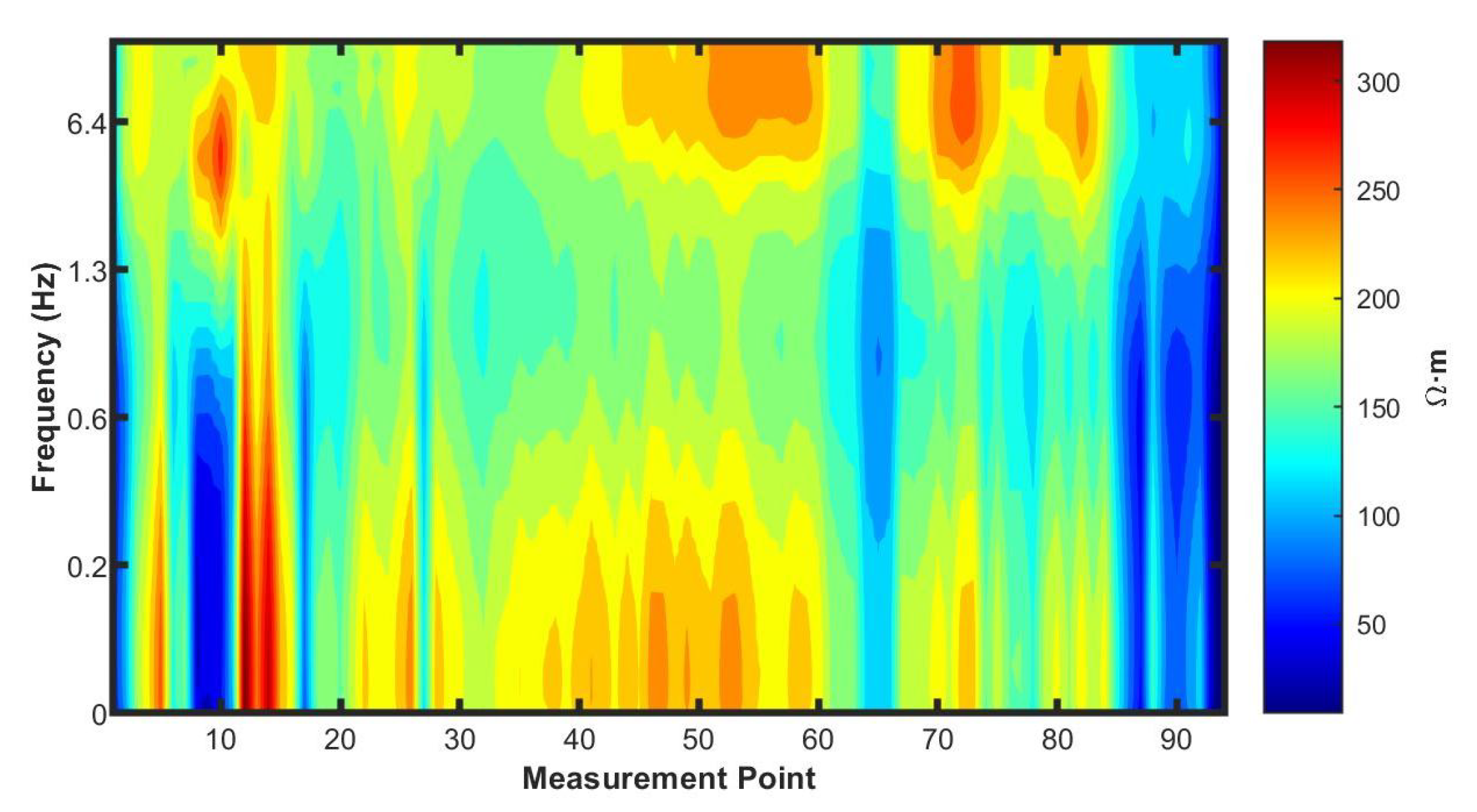
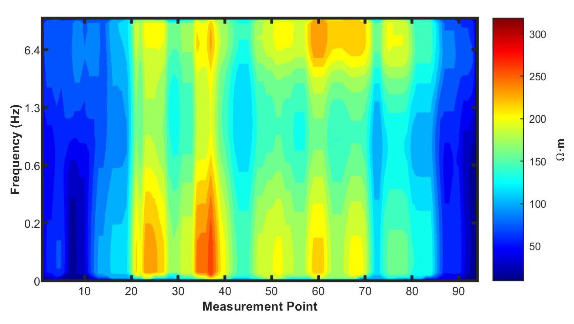
3.2. Example of Static Shift Correction on Measured Data

Figure 3 presents the time-frequency electromagnetic data acquired in a certain area. During the survey, a time-frequency electromagnetic system was used to simultaneously measure the horizontal component of the electric field and the vertical component of the magnetic field. The survey line is approximately 2 km long, with a spacing of 20 m between stations, resulting in a total of 94 measurement points. The frequency range spans from 0.05 Hz to 20 Hz. Due to the presence of near-surface inhomogeneous electrical structures within the survey area, the profile reveals numerous vertically oriented, banded anomalies.

After processing with the algorithm proposed in this paper, the results shown in Figure 4 reveal significant changes in the electrical properties near the measurement points 10 to 17, which may correspond to regions with localized electrical property discontinuities in the subsurface. Near measurement point 65, there appears to be a noticeable low-resistivity layer.

Figure 5 shows the results after applying spatial filtering correction using a $5\times 5$ window. It can be observed that due to the averaging nature of the spatial filter, some details are obscured—for example, the relatively complex electrical variations near measurement point 10 and the low-resistivity anomaly near point 65. Meanwhile, certain static displacement effects remain uncorrected, such as those near points 30–40 and around point 90.

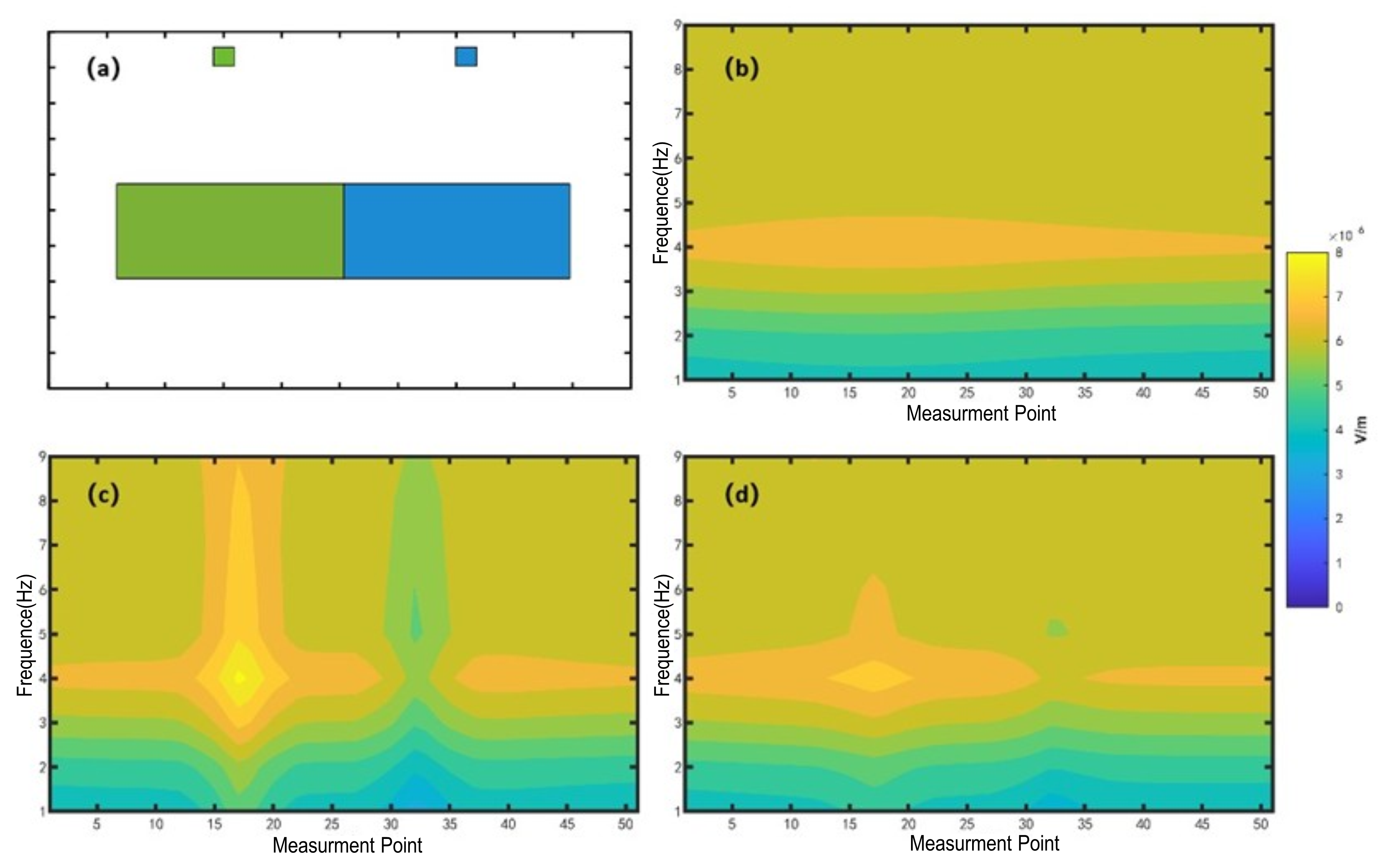
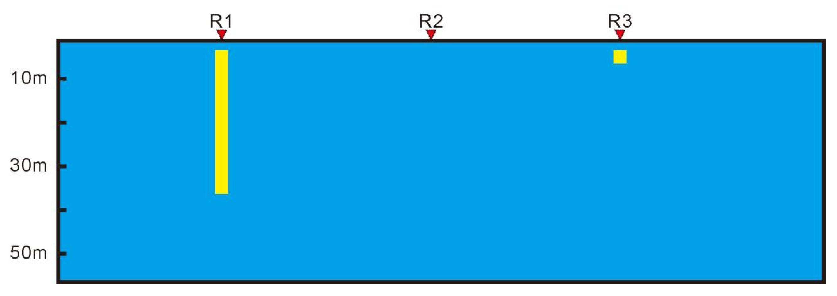
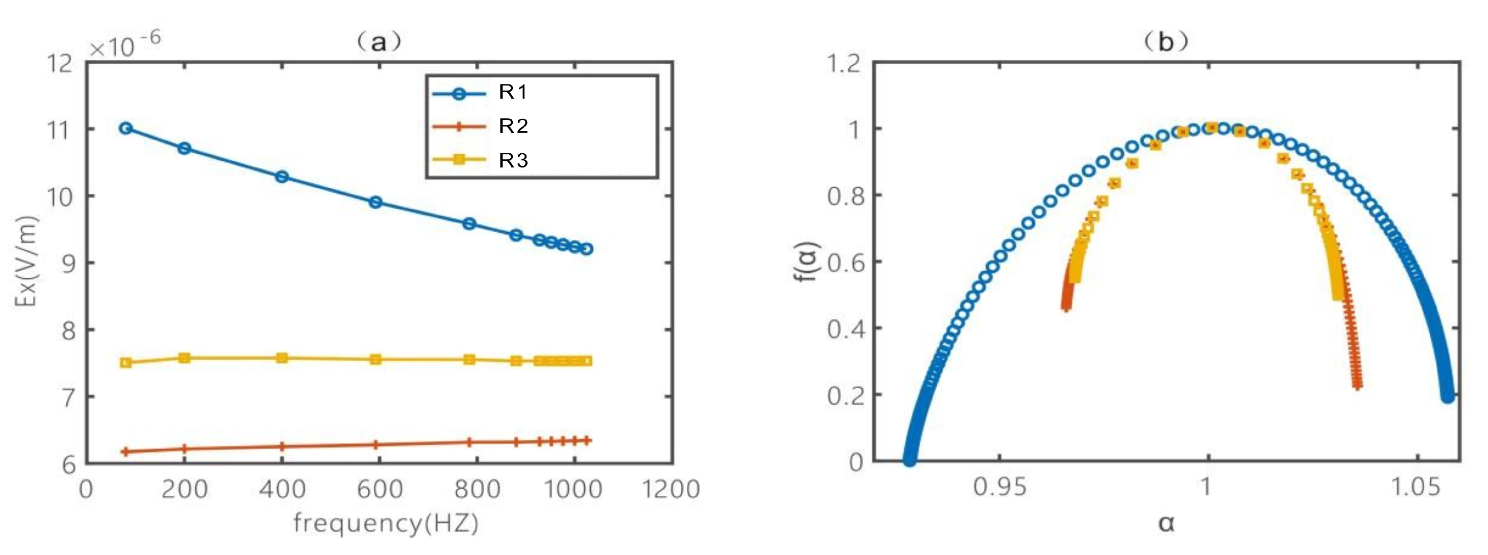
3.3. Multifractal Spectrum Analysis of Electric Field in a Simple Electrical Model

Using the two parameters in the multifractal spectrum, we can distinguish deep anomalies that are obscured by static shift effects caused by shallow inhomogeneous bodies in the electric field data and also identify magnetic field anomalies induced by shallow anomalous bodies.

A 2.5D electrical profile model is designed as follows: The plate-like anomaly has the same depth as the upper surface of the shallow anomaly, and the resistivity is the same. The locations of the measurement points are shown in Figure 6, where the TM configuration is used to measure the electric field component $E_x$ and the vertical magnetic field Hz. Figure 7a shows the curve of the components of the electric field $E_x$ component curve, and Figure 7b presents the multifractal spectrum.

In the data of Figure 7a, the electric field curves obtained at measurement points over the shallow subsurface anomaly and the vertical plate-shaped anomaly in the simple electrical model are quite similar in shape. In the presence of numerous shallow anomalies, the differentiation of them requires experience. In Figure 7b, it can be seen that the multifractal spectrum of the shallow subsurface anomaly differs very little from the case without anomalies, indicating that the resistivity anomaly of the shallow subsurface anomaly manifests primarily as a static component effect. In contrast, the multifractal spectrum of the vertical plate-like anomaly shows significant differences, reflecting the presence of a true anomaly.

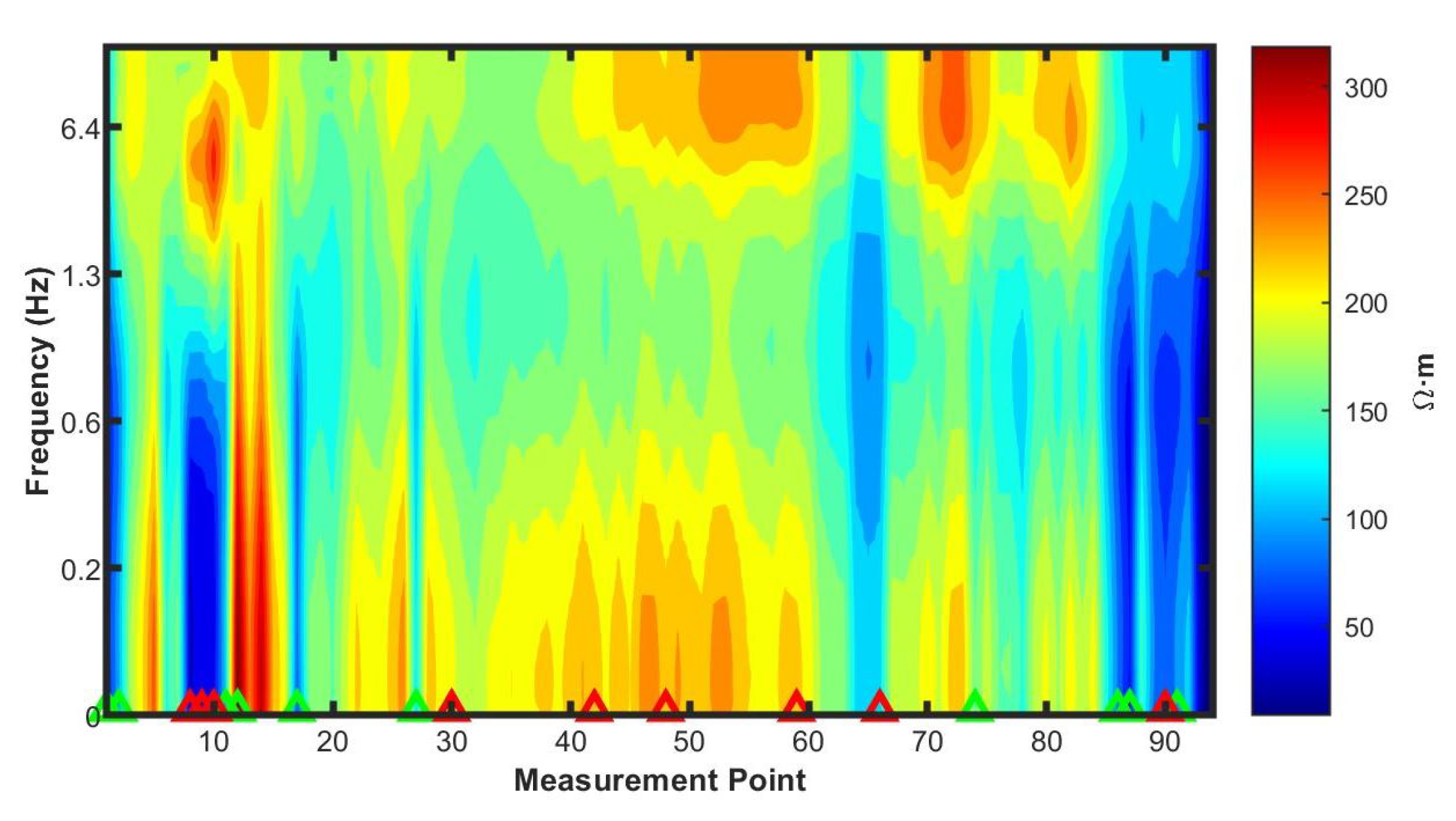
3.4. Multifractal Feature Analysis of Field Data

As previously discussed, the differences in multifractal spectra between shallow subsurface anomalies and plate-like anomalies substantiate that variations in the underlying anomalous bodies lead to different inhomogeneity and roughness characteristics in field data. We conducted a multifractal spectrum analysis on the field data before and after correction (Figure 3 and Figure 4). After correction, significant changes were observed in apparent resistivity values; however, the two multifractal scaling exponents exhibited minimal variation (Figure 8). This suggests that our static effect correction process effectively preserved the gradient variations between apparent resistivity values at different frequencies, along with information related to roughness and other inherent characteristics.

By performing a multifractal spectrum analysis on the survey line (Figure 9 and Figure 10), it can be observed that the values at both ends of the line are significantly higher than those in the middle section, indicating that the complexity of the data is higher at the ends, suggesting more complex geological conditions. Although there are numerous longitudinal strip-like anomalies in the middle section, the broadly distributed and stable low values indicate that the anomalies in this segment of the profile are primarily caused by static shift effects.

We also performed Gaussian mixture clustering in the multifractal spectrum, resulting in three categories of measurement points (Figure 11). The yellow regions are the most numerous and represent the most common data points in the profile. The cluster center of this region reflects the average data complexity of most of the measurement points. The points in the red region exhibit higher data complexity, indicating that the subsurface electrical structure beneath these points is more complex. In contrast, the points in the green region have very low complexity, suggesting a simpler subsurface electrical structure beneath these locations.

In Figure 12, we marked the high-complexity and low-complexity measurement points, as identified by clustering, on the corrected apparent resistivity profile. Red indicates high-complexity data points, and green indicates low-complexity data points. It is clearly observed that the red dots correspond to areas with more significant electrical variations, while the green dots exhibit relatively small changes in both electrical properties and frequency. This shows that the multifractal spectrum effectively distinguishes the complexity of the subsurface electrical structure in the field data.

4. Discussion

We developed a new static shift correction method tailored to the characteristics of the time-frequency electromagnetic (TFEM) technique. Combined with multifractal spectrum analysis, this approach enables a clearer understanding of the subsurface electrical structure and has been well validated on both theoretical and field datasets.

The method relies on the simultaneous measurement of horizontal electric and vertical magnetic fields at each station, which helps avoid the impact of sparse sampling and strong electrical heterogeneity near the surface. This is consistent with previous findings [14].

Multifractal spectrum analysis of the field data shows that the roughness and gradient features of the data remain largely unchanged before and after correction, indicating that the static shift correction preserves a sufficient amount of the original information. This supports earlier conclusions that static shift distortion is a global effect [1,2].

From a mathematical perspective, the multifractal spectrum is highly sensitive to the overall gradient (inhomogeneity) and smoothness (roughness) of the data. The authors envision that this characteristic could be applied to geophysical inversion algorithms in the future. During the iterative solution process, not only would the measured data values be fitted, but also the multifractal spectrum of the forward response would be matched with that of the measured data. This approach could potentially improve both the efficiency and the accuracy of the inversion process, as inversion not only considers numerical restoration, but also requires the restoration of the relative relationships between the data. Multifractal spectrum analysis provides valuable insights for further data analysis.

5. Conclusions

We proposed a new time-frequency electromagnetic static shift correction method, taking advantage of the benefits of simultaneous measurement of electromagnetic fields in the time-frequency electromagnetic method. The apparent resistivity defined by the high-frequency magnetic field is used to correct the electric field. The method was validated using field data, demonstrating that our algorithm effectively eliminates the impact of static shift effects. In addition, we discussed the applicability of the multifractal algorithm in detecting the complexity of electromagnetic field data. We showed that, after static shift correction using this method, the changes in multifractal parameters are minimal, indicating that the method preserves the complete electrical information of the subsurface while correcting for static shift. Multifractal spectrum analysis can intuitively extract subsurface electrical complexity information from electrical field or apparent resistivity data, which not only evaluates the effectiveness of static shift correction from multiple dimensions but also provides important guidance for subsequent inversion processes.

References

1. Jones, A.G. Static shift of magnetotelluric data and its removal in a sedimentary basin environment. Geophysics 1988, 53, 967–978. [Google Scholar] [CrossRef]
2. Ogawa, Y. On two-dimensional modeling of magnetotelluric field data. Surv. Geophys. 2002, 23, 251–273. [Google Scholar] [CrossRef]
3. Singer, B.S. Correction for distortions of magnetotelluric fields: Limits of validity of the static approach. Surv. Geophys. 1992, 13, 309–340. [Google Scholar] [CrossRef]
4. da Silva, M.A.S.; Nobrega, F.A.C.; do Carmo, F.F.; do Nascimento, J.P.C.; Nogueira, F.E.A.; Sales, A.J.M.; Sombra, A.S.B. Investigation of dielectric properties of a Li4Ti5O12 ceramic matrix for microwave temperature sensing applications. J. Austr. Ceram. Soc. 2024, 60, 355–362. [Google Scholar] [CrossRef]
5. Jabarov, S.H.; Nabiyeva, A.K.; Samadov, S.F.; Abiyev, A.S.; Sidorin, A.A.; Trung, N.V.M.; Orlov, O.S.; Mauyey, B.; Trukhanov, S.V.; Trukhanov, A.V. Study of defects formation mechanism in La1−xBaxMnO3 perovskite manganite by positron annihilation lifetime and Doppler broadening spectroscopy. Solid State Ion. 2024, 414, 116640. [Google Scholar] [CrossRef]
6. Bostick, F.X., Jr. Electromagnetic array profiling (EMAP). In Proceedings of the SEG Technical Program Expanded Abstracts; Society of Exploration Geophysicists: Houston, TX, USA, 1986; pp. 60–61. [Google Scholar]
7. Schultz, A.; Kurtz, R.D.; Chave, A.D.; Jones, A.G. Conductivity discontinuities in the upper mantle beneath a stable craton. Geophys. Res. Lett. 1993, 20, 2941–2944. [Google Scholar] [CrossRef]
8. Tournerie, B.; Chouteau, M. Analysis of magnetotelluric data along the Lithoprobe seismic line 21 in the Blake River Group, Abitibi, Canada. Earth Planets Space 2002, 54, 575–589. [Google Scholar] [CrossRef]
9. Torres-Verdin, C.; Bostick, F.X., Jr. Implications of the Born approximation for the magnetotelluric problem in three-dimensional environments. Geophysics 1992, 57, 587–602. [Google Scholar] [CrossRef]
10. Andrieux, P.; Wightman, W. (Eds.) The so-called static corrections in magnetotelluric measurements. In Proceedings of the SEG Technical Program Expanded Abstracts; Society of Exploration Geophysicists: Houston, TX, USA, 1984; pp. 43–44. [Google Scholar]
11. Pellerin, L.; Hohmann, G.W. Transient electromagnetic inversion: A remedy for magnetotelluric static shifts. Geophysics 1990, 55, 1242–1250. [Google Scholar] [CrossRef]
12. Sternberg, B.K.; Washburne, J.C.; Pellerin, L. Correction for the static shift in magnetotellurics using transient electromagnetic soundings. Geophysics 1988, 53, 1459–1468. [Google Scholar] [CrossRef]
13. Zhang, P.; Chouteau, M.; Mareschal, M.; Kurtz, R.; Hubert, C. High-frequency magnetotelluric investigation of crustal structure in north-central Abitibi, Quebec, Canada. Geophys. J. Int. 1995, 120, 406–418. [Google Scholar] [CrossRef]
14. Tournerie, B.; Chouteau, M.; Marcotte, D. Magnetotelluric static shift: Estimation and removal using the cokriging method. Geophysics 2007, 72, F25–F34. [Google Scholar] [CrossRef]
15. Zhanxiang, H.; Zhi, Z.; Haiying, L.; Jinchen, Q. TFEM for oil detection: Case studies. Lead. Edge 2012, 31, 518–521. [Google Scholar] [CrossRef]
16. Zhanxiang, H.; Xiaodong, S.; Zuzhi, H.; Yanling, S.; Dongyang, S.; Weibin, D. Time-frequency electromagnetic method for exploring favorable deep igneous rock targets: A case study from north Xinjiang. J. Environ. Eng. Geophys. 2019, 24, 215–224. [Google Scholar] [CrossRef]
17. Li, Z.Q.; Fu, G.Q.; Tan, S.Q.; Chen, X.G.; Guo, T.; Xiang, P.; Yang, Y.H.; He, Z.X. Calculation and application of apparent resistivity in the frequency domain by TFEM. Appl. Geophys. 2024, 21, 409–417. [Google Scholar] [CrossRef]
18. Weibin, D.; Xiaoming, Z.; Fang, L.; Guo, Z. The time-frequency electromagnetic method and its application in western China. Appl. Geophys. 2008, 5, 127–135. [Google Scholar] [CrossRef]
19. Zhang, C.H.; Liu, X.J.; He, L.F.; He, W.H.; Zhou, Y.M.; Zhu, Y.S.; Cui, Z.W.; Kuang, X.H. A study of exploration organic rich shales using Time-Frequency Electromagnetic Method (TFEM). Chin. J. Geophys. 2013, 56, 3173–3183. [Google Scholar]
20. Zhao, Z.; He, Z.X.; Li, D.C.; Yang, S.J.; Liu, X.J.; Li, T.B. Detecting favorable oil and gas targets with time-frequency electromagnetic method—Case studies. In Proceedings of the 72nd EAGE Conference and Exhibition incorporating SPE EUROPEC 2010, Amsterdam, The Netherlands, 23–26 June 2010; cp-161. [Google Scholar]
21. Asrillah, A.; Abdullah, A.; Bauer, K.; Norden, B.; Krawczyk, C.M. Fracture characterisation using 3-D seismic reflection data for advanced deep geothermal exploration in the NE German Basin. Geothermics 2024, 116, 102833. [Google Scholar] [CrossRef]
22. Gaci, S.; Nicolis, O. A grey system approach for estimating the hölderian regularity with an application to Algerian well log data. Fractal Fract. 2021, 5, 86. [Google Scholar] [CrossRef]
23. Turcotte, D.L. Fractals and Chaos in Geology and Geophysics, 2nd ed.; Cambridge University Press: Cambridge, UK, 1997. [Google Scholar]
24. Zeng, X.; Liu, T.; Tan, X.; Zhang, Y.; Li, X. Automatic determination of the cut-off wavenumber for downward continuation of potential field based on fractal radial spectrum. Prog. Geophys. 2024, 39, 403–411. [Google Scholar]
25. Zhang, X.; Li, D.; Li, J.; Liu, B.; Jiang, Q.; Wang, J. Signal-noise identification for wide field electromagnetic method data using multi-domain features and IGWO-SVM. Fractal Fract. 2022, 6, 80. [Google Scholar] [CrossRef]
26. Halsey, T.C.; Jensen, M.H.; Kadanoff, L.P.; Procaccia, I.; Shraiman, B.I. Fractal measures and their singularities: The characterization of strange sets. Phys. Rev. A 1986, 33, 1141. [Google Scholar] [CrossRef] [PubMed]
Figure 1. Flowchart of static shift correction.
Fractalfract 09 00240 g001
Figure 2. Simulation and correction of static shift in a theoretical model. (a) 2.5D geological structure profile, where green and blue represent high-resistivity and low-resistivity anomalies, respectively; (b) Theoretical forward response of the electric field without shallow anomaly bodies; (c) Forward response of the electric field with static shift effects; (d) Electric field response corrected using the proposed method.
Fractalfract 09 00240 g002
Figure 3. Original apparent resistivity profile data.
Fractalfract 09 00240 g003
Figure 4. Apparent resistivity profile after static shift correction.
Fractalfract 09 00240 g004
Figure 5. Apparent resistivity profile after spatial filtering correction.
Fractalfract 09 00240 g005
Figure 6. 2.5D profile of the geoelectric model.
Fractalfract 09 00240 g006
Figure 7. (a) Frequency-domain electric field E x components measured at points R1, R2, and R3; (b) Multifractal spectra of the frequency-domain electric field E x data at points R1, R2, and R3.
Fractalfract 09 00240 g007
Figure 8. Comparison of multifractal spectra before and after correction.
Fractalfract 09 00240 g008
Figure 9. Δ α at each measurement point in the field data.
Fractalfract 09 00240 g009
Figure 10. Δ f ( α ) at each measurement point in the field data.
Fractalfract 09 00240 g010
Figure 11. Clustering results of multifractal spectra for each measurement point in the field data.
Fractalfract 09 00240 g011
Figure 12. Measurement points with high complexity (red markers) and low complexity (green markers) as indicated by the multifractal spectra.
Fractalfract 09 00240 g012
Disclaimer/Publisher’s Note: The statements, opinions and data contained in all publications are solely those of the individual author(s) and contributor(s) and not of MDPI and/or the editor(s). MDPI and/or the editor(s) disclaim responsibility for any injury to people or property resulting from any ideas, methods, instructions or products referred to in the content.