Article

A Suitable Algorithm to Solve a Nonlinear Fractional Integro-Differential Equation with Extended Singular Kernel in (2+1) Dimensions

by
Sameeha Ali Raad
1,* and
Mohamed Abdella Abdou
2
1
Mathematics Department, Faculty of Sciences, Umm Al-Qura University, Makkah 21955, Saudi Arabia
2
Department of Mathematics, Faculty of Education, Alexandria University, Alexandria 21526, Egypt
*
Author to whom correspondence should be addressed.
Fractal Fract. 2025, 9(4), 239; https://doi.org/10.3390/fractalfract9040239
Submission received: 21 February 2025 / Revised: 30 March 2025 / Accepted: 7 April 2025 / Published: 10 April 2025

Abstract

In this paper, the authors consider a problem with comprehensive properties in terms of form and content in the space L 2 a , b × c , d × C 0 , T , T < 1 . In terms of time form, we assume that the time phase delay is implicitly contained in a nonlinear differential integral equation. The positional part is considered in two dimensions, and the position’s kernel is a general singular kernel, many different forms of which will be derived. In terms of content, all of the previously established numerical techniques are only appropriate for studying special cases of the kernel separately but are not suitable for studying the general kernel. This led to the use of the Toeplitz matrix method, which deals with the kernel in its extended nonlinear form and the special kernels will be studied as applications of the method. Moreover, this method has the advantage of converting all single integrals into regular integrals that can be easily solved. Additionally, the researchers examine the solution’s existence, uniqueness, and convergence in this paper. The error and its stability are also studied. At the end of the research, the authors studied some numerical applications of some of the singular kernels derived from the general kernel, examining the approximation error in each application separately.

1. Introduction

Interest in fractional equations and fractional integral equations has increased steadily in recent years due to their wide range of applications. The list of applications has become far more diverse and extensive in a short time. Fractional integro-differential equations (FrI-DEs) for electromagnetic waves in a dielectric medium were discovered by Tarasov [1]. Munusamy et al. [2] used the resolvent operator theory and the fixed-point theorem to examine the existence of a mild solution of the FrI-DE with nonlocal conditions. In [3], the existence of a solution to FrI-DEs was presented using the Banach principle and fixed-point theorems. After converting the Volterra–Fredholm integral equation (V-FIE) from FrI-DE using the Riemann–Liouville fractional integral, the existence of a unique solution was demonstrated using the Picard technique [4]. Alhazmi [5] employed a novel method based on the orthogonal polynomials method and variable separation to derive numerous spectral relationships from the mixed integral equation using the generalized potential kernel. The Legendre polynomials approach was used by Nemati et al. [6] to analyze the results of the second kind of two-dimensional (2D) Volterra integral model. Hafez and Youssri [7] discussed using the Legendre–Chebyshev polynomials to solve the 2D integral model numerically based on the V-FIE. The existence of solutions for a coupled system of FrI-DEs with Riemann–Stieltjes integral conditions and nonlocal infinite-point was demonstrated by El-Sayed et al. [8]. FrI-DEs can be solved in a variety of ways, some of which are analytical. Using the Taylor expansion method, Huang et al. [9] provided a simple and closed solution to a class of FrI-DEs. Legendre wavelets were used to solve a class of 2-D FrI-DEs in [10]. Using Babenko’s method, Li and Plowman developed solutions for the generalized Abel’s integral equations with variable coefficients [11]. In [12], Matoog applied the modified Taylor’s technique to derive a nonlinear algebraic system from the Hammerstein–Volterra integral equation with a continuous kernel. In order to reach the approximate solution, Abusalim et al. [13] used hybrid and block-pulse functions to solve the 2-D nonlinear integral equation with symmetric and nonsymmetric kernels. The separation of variables technique has been used to solve the mixed V-FIE [14]. By using the properties of a fractional integral, Jan [15] was able to conform the nonlinear mixed FrI-DE to the Volterra–Hammerstein integral equation. By using the extended cubic B-spline, Akram et al. [16] interpreted the collocation strategy for solving the partial FrI-DE. The approximate solution for variable-order FrI-DEs with a weakly singular kernel was obtained by Abdelkawy et al. [17] by applying the Jacobi–Gauss collocation method.
In the remainder of the paper, particularly in Section 3, the authors present a second-order nonlinear fractional differential equation under initial conditions. This equation carries physical implications, particularly since the kernel of the equation is completely singular in various ways. Under the conditions imposed on the equation, the authors were able to transform it into a mixed integral equation that is nonlinear in position and time. Also, in Section 4 of the paper, the authors consider special cases that can be derived from the imposed kernel. This section is of great importance and illustrates the overall significance of the paper in studying mixed integro-differential equations in position and time, where the kernel is generally singular in both dimensions. (This situation has not been previously investigated by researchers.) Furthermore, the compact matrix method used encompasses all special cases in a single, generalized form, which distinguishes this method from all other numerical methods. In addition, in Section 5, we use Banach’s fixed point theorem to demonstrate why the solution exists and is unique in the space L 2 ω × C 0 , T = L 2 a , b × c , d × C 0 , T under specific conditions. Additionally, we will demonstrate in Section 6 how the unique solution converges. The error convergence will be demonstrated using one of the well-known theorems in Section 7. In Section 8, a system of nonlinear Fredholm integral equations (SNFIEs) in position with a time-dependent coefficient is then obtained from the NMIE using the separation of variables method. In Section 9, the Toeplitz matrix method (TMM) on an integral equation yields a nonlinear algebraic system (NAS). We will then use Mable 18 to present numerical results based on the kernel of the equation, which takes the logarithmic kernel, Carleman function, and Cauchy form in Section 10. Additionally, the related errors will be computed.

2. Fractional Calculus

Definitions and properties of fractional calculus theory, which will be applied throughout the article, are stated in this section.
Definition 1 
([18]). The Riemann–Liouville fractional integral operator of order  p 0 with a 0 is defined as
I a p f x = 1 Γ p a x x t p 1 f t d t ,                       I a 0 f x = f x ,
where   Γ  is the gamma function.
In addition, we consider the following essential property for n 1 < β , γ n , n N
I a γ I a β h u = I a γ + β h u = 1 Γ γ + β a u u t γ + β 1 h t d t ,         ( 0 < γ + β < 1 ) .
Moreover, we consider the famous integral relation
0 t 0 τ n 1 0 τ 2 0 τ 1 h τ d τ d τ 1 d τ n 2 d τ n 1 = 1 Γ ( n ) 0 t t τ n 1 h τ d τ ,         n N .
Definition 2 
([19]). The left- and right-sided Riemann–Liouville fractional derivative of order p; ( n 1 ) p < n is
D x p a f x = 1 Γ n p d n d x n a x x t n p 1 f t d t .    
D b p x f x = 1 Γ n p d d x n x b t x n p 1 f t d t .    
Definition 3 
([19]). Caputo fractional derivative of order p;  ( n 1 ) p < n is defined as
D x p a C f x = 1 Γ n p a x x t n p 1 f ( n ) t d t .

3. Problem Formulation and Basic Equations

Due to the importance of integral equations, with their different kinds, that can be used to simulate a wide range of problems in the basic sciences, many scientists have focused a great deal of attention on presenting the solutions to these systems. These equations have played a significant role in finding the solutions by using diverse methods, which is in line with the rapid development in finding the solutions to these problems originating from many sciences. Additionally, recent developments in fractional calculus have consequences for real-world applications in viscoelasticity, bioengineering, and biology.
Kernels offer a more general framework, allowing for non-local interactions, anomalous diffusion, and memory effects. By incorporating fractional derivatives and extended kernels, one can extend Keller–Segel models to account for more complex behaviors observed in biological systems, where interactions may occur over long distances and involve memory or non-local effects (see Columbu et al. [20]).
Here, we consider a nonlinear mixed integro-fractional differential equation (NMI-FrDE) in time and position in the space L 2 [ ω ] × C 0 , T , T < 1 , under specific conditions in time.
μ 0 ψ x , y ; t + μ 1   p ψ x , y ; t t p + μ 2   p + 1 ψ x , y ; t t p + 1 = f x , y ; t + λ t ω k x ζ , y η   ψ α ζ , η ; t   d ζ d η , 0 < p < 1 ,
under the conditions
ψ x , y ; 0 = χ 1 x , y ,                   ψ x , y ; t t   t = 0 = χ 2 x , y   ,
where, for a linear type, α = 1 and for a nonlinear type, α = 2 , 3 , 4 , N . μ 0 ,   μ 1 and μ 2 are constants.
The solution to Equation (4) in the linear case was discussed by the same authors in [21].
The unknown function to be found is ψ x , y ; t , while the time function λ t and free term f x , y ; t have been identified as known continuous functions. The kernel of position k x ζ , y η has several single forms, which will be discussed.
With the aid of (4), the fractional Riemann–Liouville integral (1), and relations (2), (3) will be applied to an initial value problem (4), yielding the following nonlinear mixed integral equation (NMIE) with a singular kernel in the position term and a continuous kernel in time
μ 2   ψ x , y ; t + 0 t   μ 0   p   ( t s ) p Γ p + 1 + μ 1   ψ x , y ; s   d s = 1 Γ p + 1 0 t   ω ( t s ) p   λ s     k x ζ , y η   ψ α ζ , η ; s   d ζ d η   d s + F x , y ; t ,  
where
F x , y ; t = 1 Γ p + 1 0 t ( t τ ) p f x , y ; τ d τ + μ 1 χ 1 x , y + μ 2 χ 2 x , y . t p Γ p + 1 .      
Equation (6) will obviously meet the initial condition ψ x , y ; 0 = χ 1 x , y for t = 0 . Furthermore, this integral Equation (6) is equivalent to the NMI-FrDE (4) under consideration.

4. Special Cases from the Mixed Nonlinear Integral Equation and Its Extended Kernel

Equation (4) and the related one (6) are general formulas that include a variety of problems due to their form and kernel. These cases can be summarized as follows:
(I) 
Many special and new cases can be derived from NMI-FrDE
  • If in Equation (4), we consider μ 1 μ 0 = q p Γ ( p + 1 ) , μ 2 μ 0 = q p + 1 Γ ( p + 2 ) , after using the second order of Taylor expansion, we have the following equation
    ψ x , y ; t + q = f x , y ; t + λ t ω k x ζ , y η ψ α ζ , η ; t d ζ d η , α = 1 , 2 , , N .
Formula (8) represents a nonlinear phase-lag mixed integral equation in (2+1) dimension.
The problem of phase delay in physical and engineering sciences, especially in nonlinear thermoelastic materials, plays an important role in establishing the important properties of these materials before using them. Therefore, studying this type of problem gives researchers a great benefit over the ionic bonds of these materials with each other.
Moreover, in (8), letting α = 1 , we have the linear phase-lag mixed integral equation,
ψ x , y ; t + q = f x , y ; t + λ t ω k x ζ , y η ψ ζ , η ; t   d ζ d η .
The same equivalent equation to (9) is considered by the authors in [21].
  • If in Equation (6) α = 1 , we have the MI-FrDE in the form
μ 2 ψ x , y ; t + 0 t   μ 0 p ( t s ) p Γ p + 1 + μ 1 ψ x , y ; s   d s = 1 Γ p + 1 0 t   ( t s ) p λ s ω k x ζ , y η ψ ζ , η ; s   d ζ d η   d s + F x , y ; t .
  • If in Equation (6), μ 1 = μ 0 = 0 , and α = 1 , 2 , , N , we have an NFIE of the second kind
    μ 2 ψ x , y ; t = 1 Γ p + 1 0 t   ( t s ) p λ s ω k x ζ , y η ψ α ζ , η ; s   d ζ d η   d s + F x , y ; t ,
    where F x , y ; t in the last two cases is as in relation (7).
  • If in Equation (6), μ 2 = 0 , we have the following first kind mixed integral equation
0 t   μ 0 p ( t s ) p Γ p + 1 + μ 1 ψ x , y ; s   d s = 1 Γ p + 1 0 t   ( t s ) p λ s ω k x ζ , y η ψ α ζ , η ; s   d ζ d η   d s + 0 t t τ p f x , y ; τ d τ .
(II) 
Special cases from the kernel:
(II-1) we can consider the weak singular kernel from the general form as
Logarithmic kernel: k x ζ , y η = ln x ζ l n y η ,
Carleman kernel: k x ζ , y η = x ζ α y η β , 0 α , β < 1 ,
Logarithmic and Carleman kernel: k x ζ , y η = ln x ζ y η β .
(II-2) Cauchy singular kernel: k x ζ , y η = 1 x ζ y η ,
Cauchy–logarithmic kernel: k x ζ , y η = l n y η x ζ ,
(f) Cauchy–Carleman kernel : k x ζ , y η = l n y η x ζ .
(II-3) Strong singular kernel: k x ζ , y η = 1 x ζ 2 y η 2 .
(II-4) Super-strong singular kernel: k x ζ , y η = 1 x ζ   n y η   m , 2 < n , m N , M .

5. Existence of a Unique Solution of the Integro-Fractional Differential Equation

For this aim, we assume the following conditions:
(i)
The kernel of position k x ζ ,   y η satisfies the discontinuity conditions in the space L 2 a , b × c , d
c d c d a b a b k 2 x ζ , y η d x d ζ d y d η 1 2 M ,                   ( M   i s   a c o n s t a n t )
(ii)
The kernel ( t s ) p t ,   s [ 0 , T ] ,   0 s t T < 1 , satisfies for a continuous function λ t ,   λ t ξ , the following integrals are continuous functions of t
m a x 0 s T   0 t   ( t s ) p d s ,             τ 1 τ 2   ( t s ) p λ s d s ,             0 t   ( t s ) p λ s d s .
Consequently, we have
0 t ( t s ) p λ ( s ) d s T p + 1 ξ Γ p + 1 , p 1 .
(iii)
The norm of the function F x , y ; t in Equation (7) is defined as
F x , y ; t 1 Γ p + 1 0 t t τ p f x , y ; τ d τ + μ 1   χ 1 x , y + μ 2   χ 2 x , y t p Γ p + 1 T p + 1 f Γ p + 2 + μ 1 χ 1 x , y + μ 2 χ 2 x , y T p Γ p + 1 = Q ,
where f f . Q and f are constants.
(iv)
The known function ψ α ( x , y ; t ) , for the constant ε > m a x ε 1 , ε 2 , satisfies
i v 1       ψ α x , y ; t A 1 x , y ; t ψ x , y ; t ε 1 ψ x , y ; t ε ψ x , y ; t ,
ε 1 = m a x 0 s T 0 t c d a b A 1 2 x , y ; s   d x d y 1 2   d s ,
i v 2       ψ 1 α ( x , y ; t ) ψ 2 α ( x , y ; t ) A 2 ( x , y ; t ) ψ 1 ( x , y ; t ) ψ 2 ( x , y ; t )
ε 2 ψ 1 x , y ; t ψ 2 x , y ; t ε ψ 1 x , y ; t ψ 2 x , y ; t ,
ε 2 = m a x 0 s t 0 t c d a b A 2 2 x , y ; s   d x d y 1 2   d s ,
where A 1 x , y ; t ,   A 2 x , y ; t are continuous functions in the domain of integration.
(v)
The norm of any function h x , y ; t in L 2 a , b × c , d × C 0 , T space is defined as
h x , y ; t = max 0 t T 0 t c d a b h 2 x , y ; s d x d y 1 2   d s .
To discuss the analytic fundamentals of the NMIE (6), we write it in the integral operator form
W ¯ ψ x , y ; t = 1 μ 2 F x , y ; t + W 1 ψ x , y ; t + W 2 ψ x , y ; t ,
where
W 1 ψ x , y ; t = 1 Γ p + 1 0 t   ( t s ) p λ s c d a b k x ζ , y η ψ m   ζ , η ; s   d ζ d η   d s ,
W 2 ψ x , y ; t = 0 t   μ 0 p ( t s ) p Γ p + 1 + μ 1 ψ x , y ; s   d s .
In our study of the existence of a unique solution using the fixed-point theory or the study of the convergence of the solution as well as studying the convergence of the error, the researcher must prove that the basic integral operator in Equation (11) is finite and continuous. Therefore, it should be formulated as follows.
Lemma 1. 
The boundedness: Under the conditions (i)–(iv), the integral operators  W 1 ψ x , y ; t  and  W 2 ψ x , y ; t  are bounded. Accordingly,  W ¯ ψ x , y ; t  is also bounded. Moreover, the integral operator  W ¯ ψ x , y ; t  maps  L 2 a , b × c , d × C 0 , T —space into itself.
Proof. 
Using the relation’s norm (12), and then applying the assumptions (i)–(iv-1) with Cauchy–Schwartz inequality, we obtain
W 1 ψ x , y ; t = 1 Γ p + 1 0 t   ( t s ) p   λ s c d a b k x ζ , y η ψ α ζ , η ; s   d ζ d η   d s 1 Γ p + 1 m a x 0 s t 0 t ( t s ) p d s | λ ( t ) | c d c d a b a b k 2 x ζ , y η d x d ζ d y d η 1 2 ψ α x , y ; t ξ M T p + 1 ε Γ p + 2 max 0 s t 0 t c d a b ψ 2 ( x , y ; s ) d x d y 1 2 d s ξ M T p + 1 ε Γ p + 2 ψ ( x , y ; t ) = ρ 1 ψ x , y ; t .
However,
W 2 ψ x , y ; t = 0 t   μ 0   p ( t s ) p Γ p + 1 + μ 1     ψ x , y ; s   d s μ 0   p T p + 1 Γ p + 2 + μ 1 T ψ x , y ; t = ρ 2 ψ ( x , y ; t )
where ρ 1 = ξ   M   T p + 1 ε Γ p + 2 ,  and ρ 2 = μ 0   p T p + 1 Γ p + 2 + μ 1 T .
Therefore, use (11), with the aid of (10) to get
  W ¯ Ψ x , y ; t   1 μ 2 Q + ρ ψ x , y ; t ,                   ρ = ρ 1 + ρ 2 μ 2 .   ( μ 2 0 )
Inequality (14) indicates that the ball S r is mapped into itself by the operator W ¯ , where r = Q μ 2 ρ ,
Thus, the radius of the boundedness of convergent is
ρ = 1 μ 2 ξ   M   ε + μ 0   p T p + 1 Γ p + 2 + μ 1 T < 1 .
Lemma 2. 
The integral operator (11) is continuous under the conditions (i)–(iv).
Proof. 
Using conditions (i)–(iv), the integral operator (11) for the two functions ψ 1 x , y ; s and ψ 2 x , y ; s in the space L 2 a , b × c , d × C 0 , T leads to
W ¯ ψ 1 W ¯ ψ 2 x , y ; t 1 μ 2 0 t   μ 0   p ( t s ) p Γ p + 1 + μ 1 ψ 1 ψ 2 x , y ; s   d s + 1 μ 2 Γ ( p + 1 ) 0 t   ( t s ) p λ s c d a b k x ζ , y η ψ 1 α ψ 2 α ζ , η ; s   d ζ d η   d s 1 μ 2 0 t   μ 0 p ( t s ) p Γ p + 1 + μ 1 ψ 1 ψ 2 x , y ; s   d s + 1 μ 2 Γ ( α + 1 ) 0 t   ( t s ) p λ s c d a b k x ζ , y η ψ 1 α ψ 2 α ζ , η ; s   d ζ d η   d s     1 μ 2 ξ   M   ε + μ 0   p T p + 1 Γ p + 2 + μ 1 T ψ 1 x , y ; t ψ 2 x , y ; t ,
which can be simplified as follows:
W ¯ ψ 1 W ¯ ψ 2 x , y ; t ρ   ψ 1 x , y ; t ψ 2 x , y ; t .
Operator (11) is a continuous and bounded integral operator. Furthermore, operator (11) is a contraction mapping under the inequality (15). There, we can state the following:
Theorem 1. 
The mixed integral Equation (6), with the aid of a Banach fixed point theorem, has a unique solution, under the condition (15).
Proof. 
The proof of the theorem is directly obtained after applying Lemma 1 and Lemma 2. □

6. Stability of a General Solution

Lemma 3. 
Under the conditions (i)–(iv), the infinite series  i = 0   Ψ i ( x , y ; t ) is uniformly convergent to a continuous solution function  Ψ ( x , y ; t ) .
Proof. 
For this, construct the sequence of functions Ψ ( x , y ; t ) = Ψ 0 , Ψ 1 , , Ψ n 1 , Ψ n , = Ψ i i = 0 , then pick up two functions Ψ n 1 , Ψ n such that
μ 2 Ψ n ( x , y ; t ) + 0 t   μ 0   p ( t s ) p Γ p + 1 + μ 1   Ψ n 1 ( x , y ; s )   d s   = 1 Γ p + 1 0 t   ( t s ) p λ s c d a b k x ζ , y η Ψ n 1 α ζ , η ; s   d ζ d η   d s + F x , y ; t , μ 2 Ψ n 1 ( x , y ; t ) + 0 t   μ 0   p ( t s ) p Γ p + 1 + μ 1 Ψ n 2 ( x , y ; s )   d s = 1 Γ p + 1 0 t   ( t s ) p   λ s c d a b k x ζ , y η   Ψ n 2 α ζ , η ; s   d ζ d η   d s + F x , y ; t .
Hence, from the above we have
μ 2 Ψ n ( x , y ; t ) Ψ n 1 ( x , y ; t ) + 0 t   μ 0   p ( t s ) p Γ p + 1 + μ 1 Ψ n 1 ( x , y ; s ) Ψ n 2 ( x , y ; s )   d s
= 1 Γ p + 1 0 t   ( t s ) p   λ s c d a b k x ζ , y η Ψ n 1 α ζ , η ; s Ψ n 2 α ζ , η ; s   d ζ d η   d s .
Taking the norm, and applying conditions (i), (ii), and (iv), we follow
μ 2 Ψ n ( x , y ; t ) Ψ n 1 ( x , y ; t ) 0 t   μ 0   p ( t s ) p Γ p + 1 + μ 1 Ψ n 1 x , y ; s Ψ n 2 x , y ; s   d s + 1 Γ p + 1 0 t   ( t s ) p   λ s c d a b k x ζ , y η Ψ n 1 α ζ , η ; s Ψ n 2 α ζ , η ; s   d ζ d η   d s .
Finally, we get
Ψ n x , y ; t Ψ n 1 x , y ; t ρ   Ψ n 1 x , y ; t Ψ n 2 x , y ; t .
Now, assume
Φ n x , y ; t = Ψ n x , y ; t Ψ n 1 x , y ; t ,
hence, we have
Φ 0 x , y ; t = Ψ 0 x , y ; t = F x , y ; t μ 2 ,             Ψ n x , y ; t = i = 0 n   Φ i x , y ; t ,
using the results of Equation (18) in inequality (17), we have
Φ n x , y ; t 1 μ 2 ξ   M   ε + μ 0   p T p + 1 Γ p + 2 + μ 1 T Φ n 1 x , y ; t = ρ Φ n 1 x , y ; t .
Letting n = 1 , we have
Φ 1 x , y ; t 1 μ 2 ξ   M   ε + μ 0 p T p + 1 Γ p + 2 + μ 1 T   Q = ρ   Q .
By induction, we have
Ψ n x , y ; t Q   ρ n ,             ρ = 1 μ 2 ξ   M   ε + μ 0 p   T p + 1 Γ p + 2 + μ 1 T < 1 .
As we know
Ψ x , y ; t = lim n Ψ n x , y ; t = i = 0   Φ i x , y ; t .
Given that Q > 0 and ρ n decrease as n increases. Hence, Ψ n x , y ; t is a decreasing function. □

7. The Error Stability

When looking at approximate solutions in general, and using computer programs to determine the results, the basic idea must be understood; that is, the error in the calculation program. The behavioral matching between the error function and the unknown function must also be taken into consideration. The graph in applications will show that the two functions have the same convergence behavior.
Assume that there is a function F n x , y ; t for ψ n x , y ; t , which is an approximate solution to Equation (6), in order to illustrate the convergence of the error. Consequently, we have:
μ 2 ψ n x , y ; t + 0 t   μ 0   p ( t s ) p Γ p + 1 + μ 1   ψ n x , y ; s   d s = 1 Γ p + 1 0 t   ( t s ) p   λ s ω k x ζ , y η   ψ n α ζ , η ; s   d ζ d η   d s + F n x , y ; t .
Hence, from (6) and (20) we have
R n x , y ; t = ε μ 2 Γ p + 1 0 t   ( t s ) p   λ s ω k x ζ , y η   R n ζ , η ; s   d ζ d η   d s 1 μ 2 0 t   μ 0   p ( t s ) p Γ p + 1 + μ 1   R n x , y ; s   d s + 1 μ 2 φ n x , y ; t , p 1 , μ 2 0 ,
where
R n x , y ; t = ψ x , y ; t ψ n x , y ; t ,             φ n x , y ; t = F x , y ; t F n x , y ; t .
To discuss the error’s convergence, we perform the following: It is necessary to create the error equation sequence { E R n i x , y ; t } i = 0 . Next, the error functions { ( R n ) i x , y ; t , ( R n ) i 1 x , y ; t } are picked up so that they match Equation (21). Thus, we have
E R n i x , y ; t = 1 μ 2 φ n x , y ; t 1 μ 2 0 t   μ 0   p ( t s ) p Γ p + 1 + μ 1   E R n i 1 x , y ; s   d s + ε μ 2 Γ p + 1 0 t   ( t s ) p λ s ω k x ζ , y η   E R n i 1 ζ , η ; s   d ζ d η   d s ,
whereas
( E R n ) i x , y ; t = ( R n ) i x , y ; t ( R n ) i 1 x , y ; t ; ( E R n ) 0 x , y ; t = 1 μ 2 φ n x , y ; t ,
and
( R n ) i x , y ; t = j = 0 i ( E R n ) j x , y ; t .
With the same time and position kernels, it is clear that the error relates to the same integral equation concept. Under the same assumptions of Theorem 1, we may discuss the error’s convergence and uniqueness of the error as the following.
Lemma 4. 
Considering conditions (i)–(iv), the infinite series  i = 0 ( E R n ) i x , y ; t ,  converges uniformly to  R n .
Proof. 
Using Equation (23), taking the norm of both sides and following the same way of Lemma 3, we have
( E R n ) i x , y ; t ρ ( E R n ) i 1 x , y ; t ,             ρ = T μ 2 ξ   M   ε + μ 0 p T p Γ p + 2 + μ 1 .
By induction, we obtain
( E R n ) i x , y ; t ρ i T p + 1 f x , y , t f i x , y , t μ 2 Γ p + 2 ,
taking the sum for i = 0 , we get
i = 0 ( E R n ) i x , y ; t T p + 1 f x , y , t f i x , y , t μ 2 Γ p + 2 i = 0 ρ i .
Finally, we have
R n x , y ; t 1 ρ 1 T p + 1 f x , y , t f i x , y , t μ 2 Γ p + 2 ,
which establishes the convergence of the error under the constraint 0 < ρ < 1 . □
Lemma 5. 
As  n ,  the error  R x , y ; t 0 .
Proof. 
From inequality (26), since f x , y ; t = f u , v ; t , then the error R n x , y ; t 0 as n . This led us to conclude that the error R n x , y ; t Equation (26) has a unique representation.
Another way to prove the error’s unique representation is to write the error equation in the integral operator form. And then to prove this integral operator is bounded and maps the space of integration L 2 a , b × c , d × C 0 , T into itself. In addition, we must prove that the integral operator is continuous and contraction-mapping. □

8. Technique of Separation of Variables

The separation of variables approach is straightforward, easy to understand, easy to solve, and simple and effective. It is an idea that the dependent variable is stated in the separable form as a multiple independent function of the independent variables. Many authors were able to approximate the unknown function of integral equations using the separation of variables approach for handling the mixed integral equation solution at a certain time.
For this, assume the following forms for the known function and the unknown function, respectively,
ψ x , y ; t = ϕ x , y Υ t   , F x , y ; t = g x , y Υ t ,   Υ 0 0 ,
where T t is the known time function.
Using (27) in NMIE (6), we have
ϕ x , y μ 2 Υ t + 0 t   μ 0   p ( t s ) p Γ p + 1 + μ 1 Υ s   d s = 1 Γ p + 1 0 t   ( t s ) p   λ s Υ α s d s × c d a b k x ζ , y η   ϕ α ζ , η   d ζ d η + g x , y Υ t ,
the above formula can be adapted in the form
ϕ x , y = γ 2 t , p γ 1 t , p c d a b k x ζ , y η   ϕ α ζ , η   d ζ d η + 1 γ 1 t , p g x , y ,
where
γ 1 t , p = 1 + 1 μ 2 Υ t 0 t   μ 0   ( t s ) p Γ p + μ 1 Υ s   d s ,
γ 2 t , p = 1 μ 2 Γ p + 1 Υ ( t ) 0 t ( t s ) p   λ s Υ α s   d s .
Formula (29) represents a nonlinear Fredholm integral equation (NFIE), in two dimensions with respect to position, with coefficients depending on time and the fractional order.

9. The Toeplitz Matrix Method

The Toeplitz matrix approach for obtaining the numerical solution to the NFIE with a singular kernel is covered in this section. The goal of this approach is to produce a system of algebraic nonlinear equations that are easily solved. The Toeplitz matrix and a matrix with zero elements other than the first and end columns are the two matrices that make up the coefficient matrix.
After letting h 1 = b a N , h 2 = d c M , in Equation (29), the integral term will take the form
c d a b k x ζ , y η   ϕ α ζ , η   d ζ d η = m = M M 1 n = N N 1 m h 2 m h 2 + h 2 n h 1 n h 1 + h 1 k x ζ , y η   ϕ α ζ , η   d ζ d η .
Then, approximate the integral in the right-hand side of (31) by
m h 2 m h 2 + h 2 n h 1 n h 1 + h 1 k x ζ , y η   ϕ α ζ , η   d ζ d η = x , y ϕ α n h 1 , m h 2 + ¯ x , y × ϕ α n h 1 , m + 1 h 2 + ^ x , y ϕ α n + 1 h 1 , m h 2 + ~ x , y ϕ α n + 1 h 1 , m + 1 h 2 + R ,
where R is the estimate error; the weights of the integration , ¯ , ^ , and ~ are continuous functions and will be determined. Using the principal idea of the Toeplitz matrix method, by assuming in (32), ϕ x , y = 1 , x , y , x y respectively, in this case R = 0 , hence, we have four formulas
I 1 x = m h 2 m h 2 + h 2 n h 1 n h 1 + h 1 k x ζ , y η   d ζ d η = + ¯ + ^ + ~ , I 2 x = m h 2 m h 2 + h 2 n h 1 n h 1 + h 1 ζ α k x ζ , y η   d ζ d η = n h 1 α + ¯ + n h 1 + h 1 α ^ + ~ , I 3 x = m h 2 m h 2 + h 2 n h 1 n h 1 + h 1 η α k x ζ , y η   d ζ d η = m h 2 α + ^ + m h 2 + h 2 α ¯ + ~ , I 4 x = m h 2 m h 2 + h 2 n h 1 n h 1 + h 1 ζ α   η α k x ζ , y η   d ζ d η = n h 1 m h 2 α     + n h 1 m + 1 h 2 α ¯ + m h 2 n + 1 h 1 α ^ + n + 1 h 1 m + 1 h 2 α ~ .
Now, by evaluating integrals, it is simple to compute weights , ¯ , ^ , and ~ immediately
x , y = m α n α + n α + m α + 1 h 1 α   h 2 α   I 1 m α + 1   h 2 α   I 2 n α + 1 h 1 α   I 3 + I 4 h 1 α   h 2 α ,
¯ x , y = n α + 1 m α h 1 α   h 2 α   I 1 + m α   h 2 α   I 2 + n α + 1 h 1 α I 3 I 4 h 1 α   h 2 α ,
^ x , y = m α + 1 n α h 1 α   h 2 α   I 1 + m α + 1   h 2 α   I 2 + n α h 1 α   I 3 I 4 h 1 α   h 2 α ,
and
~ x , y = m α n α h 1 α   h 2 α   I 1 m α h 2 α   I 2 n α   h 1 α   I 3 + I 4 h 1 α   h 2 α .
Integral Equation (32), after putting x = m   h , becomes
c d a b k x ζ , y η ψ α ζ , η   d ζ d η = m = M M n = N N Y N , n ; M , m   ψ α n h 1 , m h 2 ,
where
Y N , n ; M , m = n , m + ¯ n , m 1                                                                                                                                         ,         n = N                               n , m + ^ n 1 , m                                                                                                                                       ,         m = M                                 n , m + ¯ n , m 1 + ^ n 1 , m + ~ n 1 , m 1     ,     N < n < N , M < m < M ¯ n , m 1 + ~ n 1 , m 1                                                                                                                           ,         m = M                                   ^ n 1 , m + ~ n 1 , m 1                                                                                                                           ,         n = N .                                      
Hence, Equation (29), will be
ϕ i h 1 , j h 2 = γ 2 t , p γ 1 t , p m = M M n = N N Y N , n ; M , m   ϕ α n h 1 , m h 2 + 1 γ 1 t , p g i h 1 , j h 2 , N i N , M j M .
Formula (36) represents a nonlinear system of algebraic equations, where ϕ is a matrix of 2 N + 1 × 2 M + 1 elements, while Y N , n ; M , m elements are given by
Y N , n ; M , m = Z n , m i , j V n , m i , j
where
Z n , m i , j = n , m + ¯ n , m 1 + ^ n 1 , m + ~ n 1 , m 1     ,             N n N , M m M ,
and
V n , m i , j =   ¯ n , m 1 + ^ n 1 , m + ~ n 1 , m 1                                           ,         n = N ,   m = M   ^ n 1 , m + ~ n 1 , m 1                                                                                     ,         n = N ,   m M   ¯ n , m 1 + ~ n 1 , m 1                                                                                     ,         m = M ,   n N                                       0                                                                                       ,         N < n < N , M < m < M n 1 , m + ^ n 1 , m 1                                                                                     ,     m = M ,         n N                   n 1 , m + ¯ n , m 1                                                                                             ,     n = N ,         m M                   n 1 , m + ¯ n , m 1 + ^ n 1 , m 1                                               ,         n = N ,   m = M ,                  
here, Z n , m i , j is the Toeplitz matrix, whereas V n , m i , j is a zero matrix except the first and last rows and columns. Both matrices are of order 2 N + 1 × 2 M + 1 .
Hence, the system (35) will be reduced to the matrices form
Φ = γ 2 t , p γ 1 t , p Z + V   Φ α + 1 γ 1 t , p G   .
The nonlinear system (40) can be solved easily by Newton’s method, Broyden’s method, and the finite difference method.
The error term R is determined from Equation (32) by letting Φ x , y = x . y 2 to get
R = | m h 2 m h 2 + h 2 n h 1 n h 1 + h 1 k x ζ , y η ( ζ . η ) 2 α   d ζ d η x , y n h 1 . m h 2 2 α ¯ x , y n h 1 . m + 1 h 2 2 α ^ x , y n + 1 h 1 . m h 2 2 α ~ x , y n + 1 h 1 . ( m + 1 ) h 2 2 α | .

10. Numerical Results
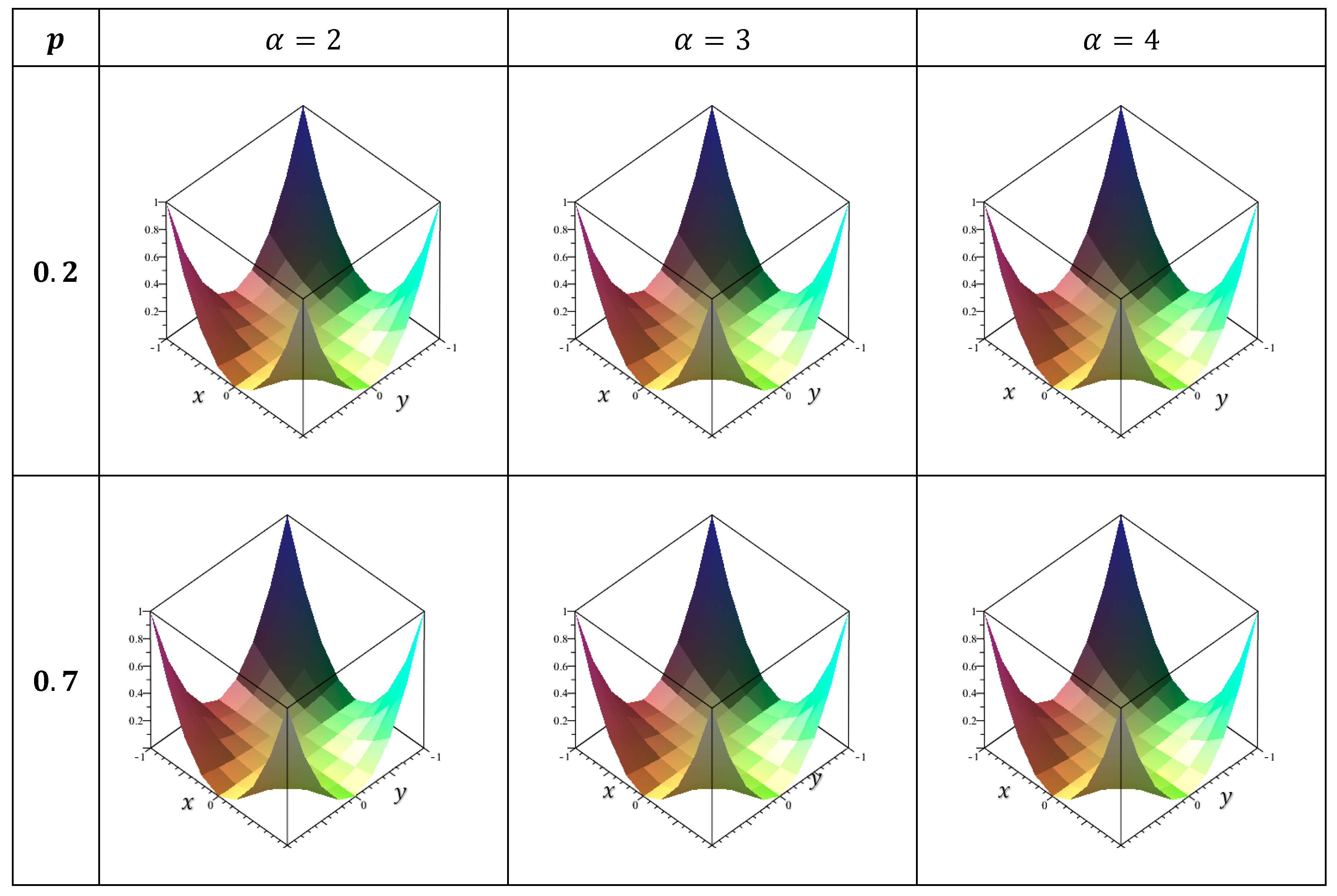
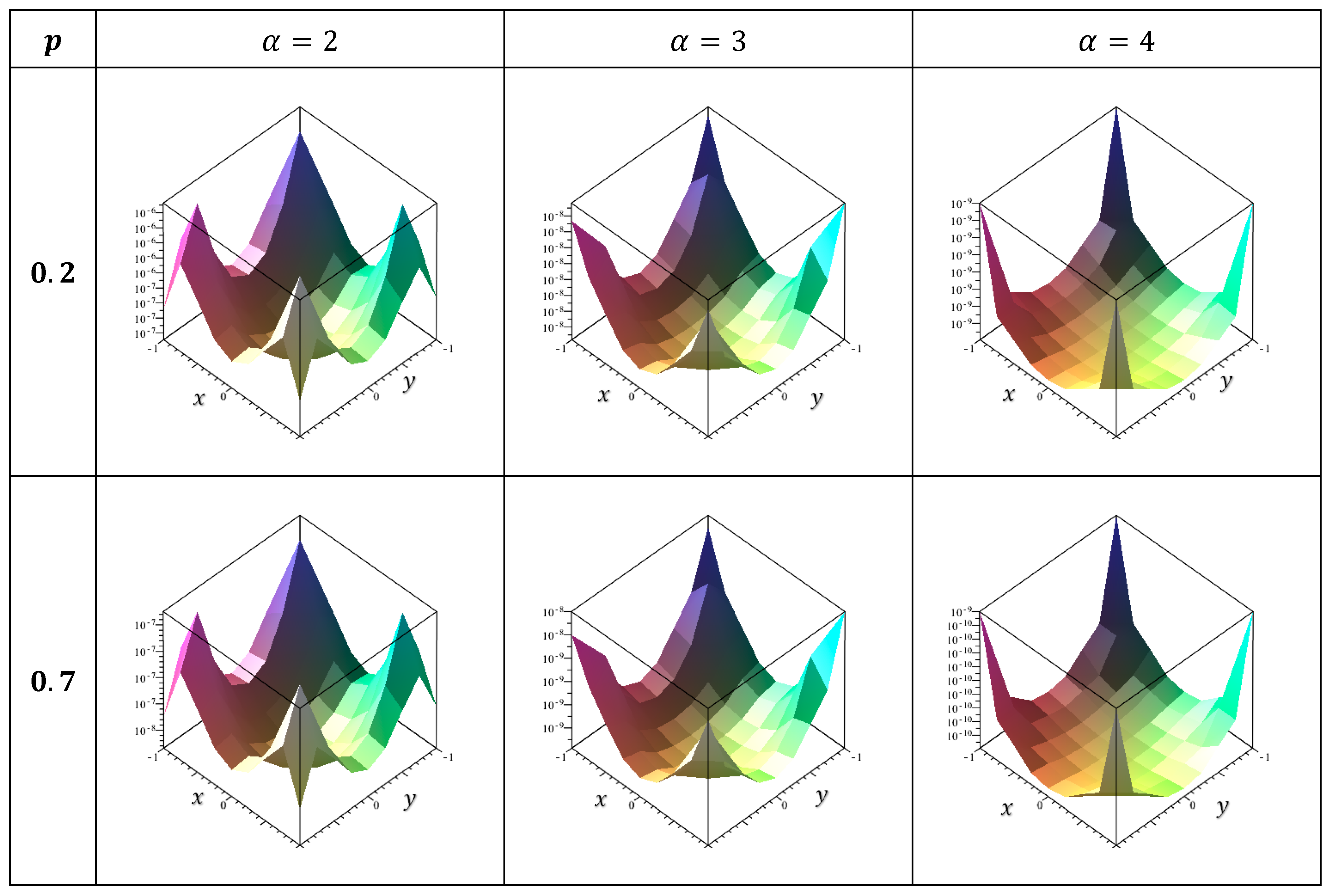
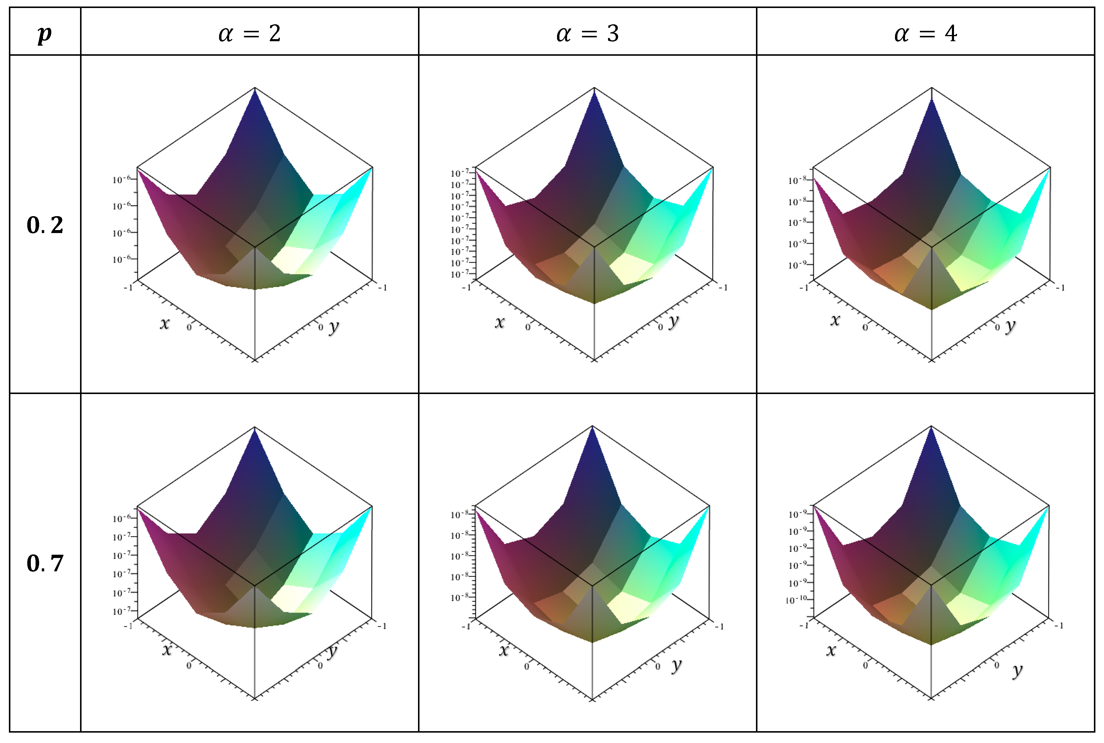
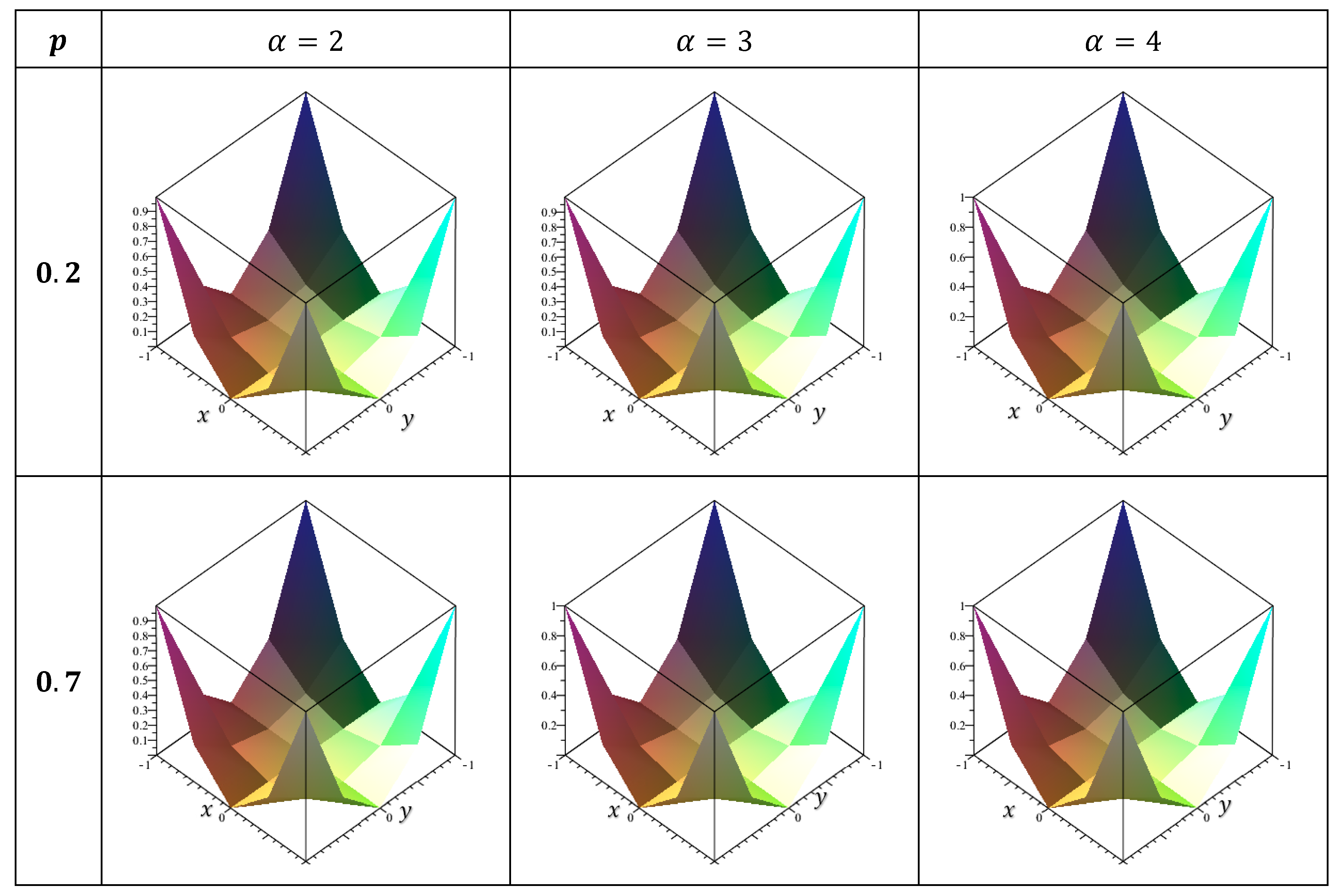
This section presents three applications that demonstrate the effects of the proposed methods on the solution of singular NMI-FrDE (4). We considered NMI-FrDE (4) with singular kernels. The algebraic system was solved numerically using the Toeplitz matrix approach. Maple18 software was used to calculate the results, accounting for the parameters μ 0 = 1 , μ 1 = 1 4 , and μ 2 = 1 2 . The exact solution is ψ x , y ; t = x 2 y 2 ( t + 0.1 ) 3 , h ( t ) = ( t + 0.1 ) 3 ,   λ ( t ) = t 2 . n = 25 units will be used to split the position plane. Numerical solutions (Num. solution) and their corresponding errors (Error) that are represented by the absolute difference between the exact solution and the numerical solution at each point ( ψ x , y ; t N u m . s o l u t i o n ), are shown at different points ( x , y ) [ 1,1 ] × [ 1,1 ] for t = 0.1 , in Table 1, Table 2, Table 3 and Table 4. Figure 1, Figure 2, Figure 3, Figure 4, Figure 5, Figure 6, Figure 7 and Figure 8 show the approximate solutions and the associated error behavior.
Application 1: Logarithmic kernel:
Consider NMI-FrDE equation with logarithmic kernel
ψ x , y ; t + 1 4 p ψ x , y ; t t p + 1 2 p + 1 ψ x , y ; t t p + 1 = f x , y ; t + t 2 1 1 1 1 ln x ζ ln y η   ψ α ζ , η ; t d ζ d η ,             α = 2 , 3 , 4 ,
under the conditions
ψ x , y ; 0 = x 2 y 2 ,             ψ x , y ; t t   t = 0 = x 2 y 2 3 .
Equation (42) can be rewritten with the aid of (43) in the form of the NMIE in
1 2 ψ x , y ; t + 0 t   p ( t s ) p Γ p + 1 + 1 4 ψ x , y ; s   d s = 1 Γ p + 1 0 t   ( t s ) p   s 2 1 1 1 1 ln x ζ ln y η   ψ α ζ , η ; t   d ζ d η   d s + F x , y ; t ,
where
F x , y ; t = 1 Γ p + 1 0 t t τ p f x , y ; τ d τ + 1 2 x 2 y 2 1 + 3   t p Γ p + 1 .
The integrals in relations (33) according to the logarithmic kernel type can be evaluated using the famous formula (see Gradshteyn and Ryzhik [22]).
u n ln ( a + b u ) d u = 1 n + 1 u n + 1 ( a ) n + 1 b n + 1 ln ( a + b u ) + k = 1 n + 1 ( 1 ) k u n k + 2 a k 1 ( n k + 2 ) b k 1 .
Application 2: Carleman kernel:
Consider NMI-FrDE equation with Carleman kernel
ψ x , y ; t + 1 4   p ψ x , y ; t t p + 1 2   p + 1 ψ x , y ; t t p + 1 = f x , y ; t + t 2 1 1 1 1   x ζ β y η γ   ψ α ζ , η ; t   d ζ d η ,               α = 2 , 3 , 4 ,
under the conditions (43).
Equation (47) can be rewritten with the aid of (43) in the form of a NMIE in
1 2   ψ x , y ; t + 0 t   p   ( t s ) p Γ p + 1 + 1 4   ψ x , y ; s   d s = 1 Γ p + 1 0 t   ( t s ) p   s 2 1 1 1 1   x ζ β x ζ γ   ψ α ζ , η ; t   d ζ d η   d s + F x , y ; t ,  
where F x , y ; t takes the form (45).
Integrals in (33) can be calculated for the Carleman function based on the formula
u n x u α d u = k = 0 n n !   u n k x u k + 1 α n k ! 1 α 2 α k + 1 α .
Application 3: Cauchy kernel:
Consider the NMI-FrDE equation with the Cauchy kernel
ψ x , y ; t + 1 4   p ψ x , y ; t t p + 1 2   p + 1 ψ x , y ; t t p + 1 = f x , y ; t + t 2 1 1 1 1     ψ α ζ , η ; t x ζ y η   d ζ d η ,               α = 2 , 3 , 4
under the conditions (43).
Equation (50) can be rewritten with the aid of (43) in the form of a NMIE in
1 2   ψ x , y ; t + 0 t   p   ( t s ) p Γ p + 1 + 1 4   ψ x , y ; s   d s = 1 Γ p + 1 0 t   ( t s ) p   s 2 1 1 1 1   ψ α ζ , η ; t x ζ y η     d ζ d η   d s + F x , y ; t ,
where F x , y ; t takes the form (45).
Integrals in (33) can be calculated for the Cauchy kernel based on the formula
u n a + b u d u =   ( a ) n b n + 1 ln a + b u 1 b k = 1 n ( 1 ) k u n k + 1 a k 1 n k + 1 b k 1   .

11. Discussion

Based on the results of previous applications, we can observe that
1.
The numerical solutions were consistently extremely near to the exact solution.
2.
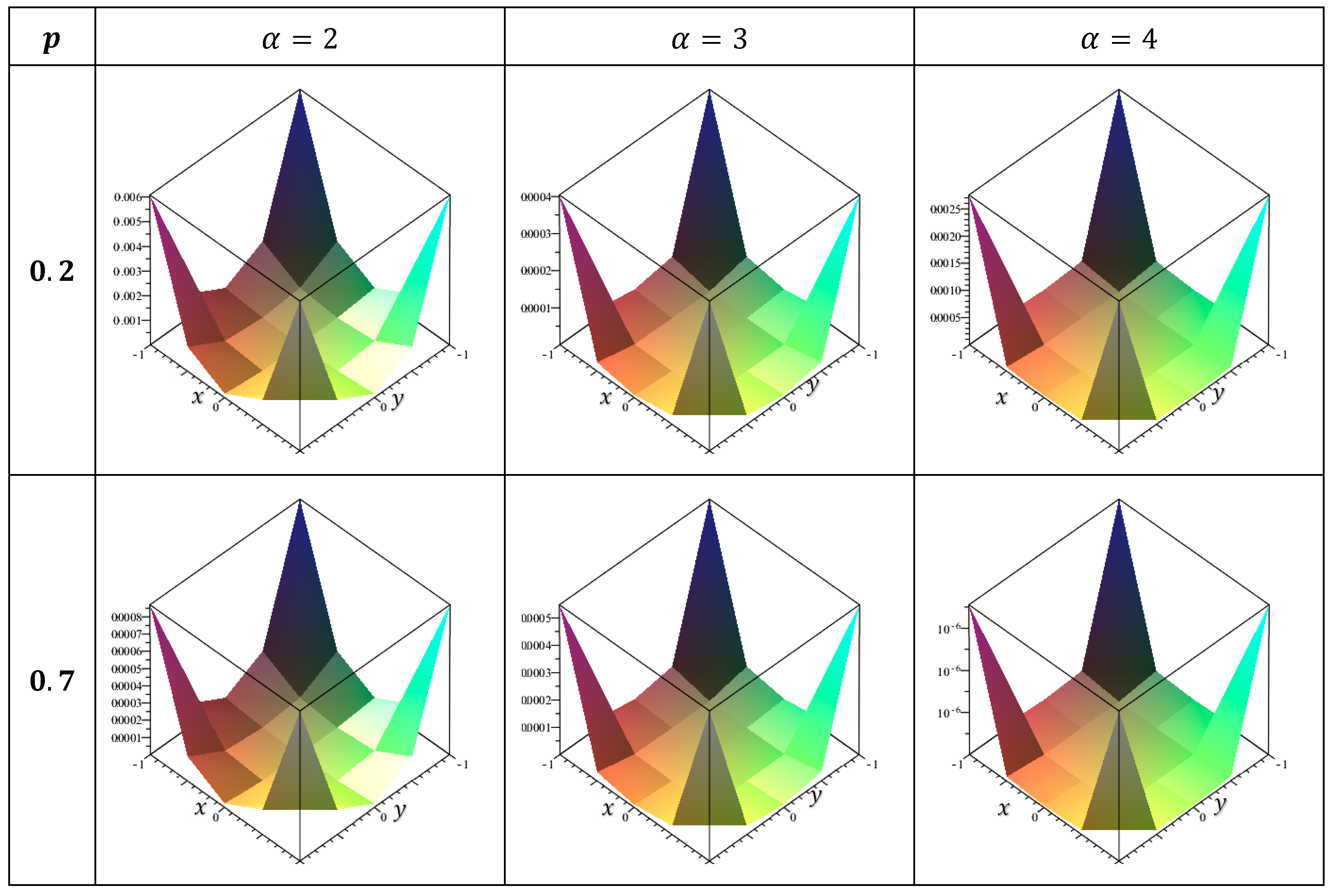
In each case studied, the error value increases as it approaches the endpoints x , y = ± 1 . Additionally, it decreases as it approaches zero at the center of the position plane.
3.
The smaller the error is, the greater is the value of α.
4.
It is clear from comparing the corresponding results of Table 2 and Table 3 that as the Carleman parameter becomes larger, the error correspondingly increases.
5.
The error decreases as the p-value increases, indicating that the accuracy in nonlinear cases is greater than the accuracy in linear cases.
6.
TMM is regarded as one of the greatest techniques for solving singular integral equations, where the solution can be obtained directly, and the singularity vanishes.
7.
The logarithmic results in Table 1 are the most accurate.
8.
The Cauchy results in Table 4 have the greatest error.
9.
The techniques used in this study preserve the symmetry characteristic of the numerical results related to the plane of position.
10.
The behavior of numerical solutions was described in Figure 1, Figure 3, Figure 5 and Figure 7. However, the corresponding errors behavior is displayed in Figure 2, Figure 4, Figure 6 and Figure 8.

12. Conclusions

From the previous study, we can deduce the following:
1.
The fractional integro-differential equation is equivalent to the phase-lag integral equation.
2.
Discussing the existence and uniqueness of the solution as well as the convergence and stability of the error is very important in discussing mathematical problems in general.
3.
In this work, special cases were derived from the general situation of the fractional integro-differential equation, and the linear relationship of the equation was also deduced from the general equation. In addition, many and various specific types were obtained from the general kernel.
4.
The investigation of the existence of a solution to the problem is classified according to the general situation of the equation to be solved and then the basic conditions for this solution: (a) Banach’s fixed point theorem must be used if the integral equation that is to be solved is of the first kind. In this case, the so-called Picard method (the method of successive approximation) fails. A theorems successive approximation approach or fixed-point theorems may be used if the equation is of the second kind. Fixed point theorems are governed by the initial conditions set to solve the problem.
5.
The Toeplitz matrix method is distinguished from all previous methods by the following properties: (a) The ability to formulate the kernel in general and to consider that the singular kernels such as the logarithmic kernel, the Caleman kernel, the Cauchy kernel, the Hilbert kernel, and finally the strongly singular kernel are special cases of the imposed kernel. (b) This method transforms the singular integrals into ordinary integrals that are easy to solve.

13. Future Work

The authors look forward to solving this type of equation in the future.
μ 0 ψ x , y ; t + μ 1   p ψ x , y ; t t p + μ 2   p + 1 ψ x , y ; t t p + 1 = f x , y ; t + L t ω k x ζ , y η   ψ α ζ , η ; t   d ζ d η ,     0 < p < 1 ,
where
L t = 0 t g ( t , τ ) ψ x , y ; τ d τ .

Author Contributions

Methodology, S.A.R. and M.A.A.; Software, S.A.R.; Formal analysis, M.A.A.; Investigation, M.A.A.; Writing—original draft, S.A.R.; Writing—review and editing, S.A.R. and M.A.A.; Project administration, M.A.A.; Funding acquisition, S.A.R. All authors have read and agreed to the published version of the manuscript.

Funding

This research work was funded by Umm Al-Qura University, Saudi Arabia, under grant number: 25UQU4280427GSSR01.

Data Availability Statement

The original contributions presented in this study are included in the article. Further inquiries can be directed to the corresponding author.

Acknowledgments

The authors extend their appreciation to Umm Al-Qura University, Saudi Arabia, for funding this research work through grant number: 25UQU4280427GSSR01.

Conflicts of Interest

The authors declare no conflict of interest.

Abbreviations

The following abbreviations are used in this manuscript:
NFIEnonlinear Fredholm integral equation
V-FIEVolterra–Fredholm integral equation
NMIEnonlinear mixed integral equation
FrI-DEsfractional integro-differential equations
NMI-FrDEnonlinear mixed integro-fractional differential equation
SNFIEssystem of nonlinear Fredholm integral equations
TMMToeplitz matrix method
NASnonlinear algebraic system

References

  1. Tarasov, V.E. Fractional integro-differential equations for electromagnetic waves in dielectric media. Theor. Math. Phys. 2009, 158, 355–359. [Google Scholar] [CrossRef]
  2. Munusamy, K.; Ravichandran, C.; Nisar, K.S.; Ghanbari, B. Existence of solutions for some functional integrodifferential equations with nonlocal conditions. Math. Methods Appl. Sci. 2020, 43, 10319–10331. [Google Scholar] [CrossRef]
  3. Verma, P.; Kumar, M. An analytical solution with existence and uniqueness conditions for fractional integro-differential equations. Int. J. Model. Simul. Sci. Comput. 2020, 11, 2050045. [Google Scholar] [CrossRef]
  4. Raad, S.; Alqurashi, K. Toeplitz matrix and Nyström method for solving linear fractional integro-differential equation. Eur. J. Pure Appl. Math. 2022, 15, 796–809. [Google Scholar] [CrossRef]
  5. Alhazmi, S.E. New model for solving mixed integral equation of the first kind with generalized potential kernel. J. Math. Res. 2017, 9, 18–29. [Google Scholar] [CrossRef]
  6. Nemati, S.; Lima, P.M.; Ordokhani, Y. Numerical solution of a class of two dimensional nonlinear Volterra integral equations using Legendre polynomials. J. Comput. Appl. Math. 2013, 242, 53–69. [Google Scholar] [CrossRef]
  7. Hafez, R.M.; Youssri, Y.H. Spectral Legendre-Chebyshev treatment of 2D linear and nonlinear mixed Volterra-Fredholm integral equation. Math. Sci. Lett. 2020, 9, 37–47. [Google Scholar]
  8. El-Sayed, A.M.A.; Ahmed, R.G. Solvability of a coupled system of functional integro-differential equations with infinite point and Riemann–Stieltjes integral conditions. Appl. Math. Comput. 2020, 370, 124918. [Google Scholar] [CrossRef]
  9. Huang, L.; Li, X.F.; Zhao, Y.; Duan, X.Y. Approximate solution of fractional integro-differential equations by Taylor expansion method. Comput. Math. Appl. 2011, 62, 1127–1134. [Google Scholar] [CrossRef]
  10. Mojahedfar, M.; Tari Marzabad, A. Solving two-dimensional fractional integrod ifferential equations by Legendre wavelets. Bull. Iran. Math. Soc. 2017, 43, 2419–2435. [Google Scholar]
  11. Li, C.; Plowman, H. Solutions of the generalized Abel’s integral equations of the second kind with variable coefficients. Axioms 2019, 8, 137. [Google Scholar] [CrossRef]
  12. Matoog, R.T. Modified Taylor’s method and nonlinear mixed integral equation. Univ. J. Integ. Eq. 2016, 4, 21–29. [Google Scholar]
  13. Abusalim, S.M.; Abdou, M.A.; Abdel-Aty, M.A.; Nili, M.E. Hybrid Functions Approach via Nonlinear Integral Equations with Symmetric and Nonsymmetrical Kernel in Two Dimensions. Symmetry 2023, 15, 1408. [Google Scholar] [CrossRef]
  14. Mahdy, A.M.S.; Abdou, M.A.; Mohamed, D.S. A computational technique for computing second-type mixed integral equations with singular kernels. J. Math. Comput. Sci. 2024, 32, 137–151. [Google Scholar] [CrossRef]
  15. Jan, A.R.; Abdou, M.A.; Basseem, M. A Physical Phenomenon for the Frac tional Nonlinear Mixed Integro-Differential Equation Using a Quadrature Nystrom Method. Fractal Fract. 2023, 7, 656. [Google Scholar] [CrossRef]
  16. Akram, T.; Ali, Z.; Rabiei, F.; Shah, K.; Kumam, P.A. Numerical Study of Nonlinear Fractional Order Partial Integro-Differential Equation with a Weakly Singular Kernel. Fractal Fract. 2021, 5, 85. [Google Scholar] [CrossRef]
  17. Abdelkawy, M.A.; Amin, A.Z.; Lopes, A.M.; Hashim, I.; Babatin, M.M. Shifted fractional-order Jacobi collocation method for solving variable-order fractional integro differential equation with weakly singular kernel. Fractal Fract. 2022, 6, 19. [Google Scholar] [CrossRef]
  18. Tariboon, J.; Ntouyas, S.K.; Sudsutad, W. Some new Riemann-Liouville fractional integral inequalities. Int. J. Math. Math. Sci. 2014, 2014, 6. [Google Scholar] [CrossRef]
  19. Podlubny, I.; Chechkin, A.; Skovranek, T.; Chen, Y.; Jara, B.M.V. Matrix approach to discrete fractional calculus II: Partial fractional differential equations. J. Comput. Phys. 2009, 228, 3137–3153. [Google Scholar] [CrossRef]
  20. Columbu, A.; Fuentes, R.D.; Frassu, S. Uniform-in-time boundedness in a class of local and nonlocal nonlinear attraction-repulsion chemotaxis models with logistics. arXiv 2023, arXiv:2311.06526. [Google Scholar] [CrossRef]
  21. Raad, S.A.; Abdou, M.A. The Effect of Fractional Order of Time Phase Delay via a Mixed Integral Equation in (2+1) Dimensions with an Extended Discontinuous Kernel. Symmetry 2025, 17, 36. [Google Scholar] [CrossRef]
  22. Gradshteyn, I.S.; Ryzhik, I.M. Table of Integrals, Series and Product; Academic Press: New York, NY, USA, 2014. [Google Scholar]
Figure 1. The numerical solution at T = 0.1 for α = 2 , 3 , 4 , according to p = 0.2 , 0.7 .
Fractalfract 09 00239 g001
Figure 2. The errors graph at T = 0.1 for p = 0.2 , 0.7 , corresponding to α = 2 , 3 , 4 .
Fractalfract 09 00239 g002
Figure 3. Using the Carlean parameter β = γ = 0.35 , the approximate solutions at T = 0.1 for p = 0.2 , 0.7 , α = 2 , 3 , 4 .
Fractalfract 09 00239 g003
Figure 4. The absolute errors at T = 0.1 for p = 0.2 , 0.7 , α = 2 , 3 , 4 , related to the Carlean parameter β = γ = 0.35 .
Fractalfract 09 00239 g004
Figure 5. The numerical solution according to the Carlean parameter β = γ = 0.6 , for p = 0.2 , 0.7 , and α = 2 , 3 , 4 , at T = 0.1 .
Fractalfract 09 00239 g005
Figure 6. The absolute errors connected to the Carlean parameter β = γ = 0.6 , at T = 0.1 for p = 0.2 , 0.7 , and α = 2 , 3 , 4 .
Fractalfract 09 00239 g006
Figure 7. The computational solution provided for α = 2 , 3 , 4 , at T = 0.1 for p = 0.2 , 0.7 .
Fractalfract 09 00239 g007
Figure 8. The absolute errors associated with α = 2 , 3 , 4 at T = 0.1 for p = 0.2 , 0.7 .
Fractalfract 09 00239 g008
Table 1. The approximate solution when p = 0.2 , 0.7 together with the associated errors.
p ( x , y ) α = 2 α = 3 α = 4
Num. SolutionErrorNum. SolutionErrorNum. SolutionError
0.2 ( ± 1 , ± 1 ) 1.000000522 5.220 × 10⁻⁷ 1.000000077 7.700 × 10⁻⁸ 1.000000008 8.10 × 10⁻⁹
( ± 0.5 , ± 1 )
( ± 1 , ± 0.5 )
0.249999061 9.394 × 10−70.24999996723.270 × 10−8 0.2499999986 1.40 × 10⁻⁹
( 0.0,0.0 ) 1.1080   × 10−71.1080 × 10−71.9989 × 10−91.9989 × 10−95.1466 × 10−11 5.1466 × 10⁻¹¹
( 0.0 , ± 1 )
( ± 1,0.0 )
4.6546   × 10−7 4.6546 × 10⁻⁷ 1.3755   × 10−8 1.3755   × 10−85.0681 × 10−105.0681 × 10⁻¹⁰
( 0.0 , ± 0.5 )
( ± 0.5,0.0 )
2.6177   × 10−7 2.6177 × 10⁻⁷ 5.1614 × 10⁻⁹ 5.1614 × 10−91.4415 × 10−101.4415 × 10⁻¹⁰
( ± 0.5 , ± 0.5 ) 0.062499392 6.0847 × 10⁻⁷ 0.062499867 1.328 × 10−80.06249999964.00 × 10−10
0.7 ( ± 1 , ± 1 ) 1.000000076 7.600 × 10⁻⁸ 1.000000010 1.100 × 10⁻⁸ 1.000000001 1.00 × 10⁻⁹
( ± 0.5 , ± 1 )
( ± 1 , ± 0.5 )
0.249999865 1.348 × 10−70.2499999964.400 × 10−9 0.249999999 2.00 × 10⁻¹⁰
( 0.0,0.0 ) 1.5829 × 10−81.5829 × 10−82.7112 × 10−102.7112 × 10−106.6448 × 10−126.6448 × 10⁻¹²
( 0.0 , ± 1 )
( ± 1 , 0.0 )
6.6495 × 10−86.6495 × 10−8 1.8656   × 10−9 1.8656   × 10−96.5434 × 10−116.5434 × 10⁻¹¹
( 0.0 , ± 0.5 )
( ± 0.5,0.0 )
3.7396   × 10−8 3.7396   × 10−8 7.0004 × 10⁻¹⁰ 7.0004 × 10−101.8611 × 10−111.8611 × 10⁻¹¹
( ± 0.5 , ± 0.5 ) 0.062499913 8.693 × 10⁻⁸ 0.062499998 1.8100 × 10−90.06249999996.00 × 10−11
Table 2. The numerical solutions for p = 0.2 , 0.7 , and β = γ = 0.35 in conjunction with the relevant errors.
p ( x , y ) α = 2 α = 3 α = 4
Num. Sol.ErrorNum. Sol.ErrorNum. Sol.Error
0.2 ( ± 1 , ± 1 ) 0.999992630 7.3700 × 10⁻⁶ 0.999999696 3.0450 × 10⁻⁷ 0.999999986 1.4200 × 10⁻⁸
( ± 0.5 , ± 1 )
( ± 1 , ± 0.5 )
0.249994314 5.6863 × 10−60.24999979212.0540 × 10−70.2499999918.9000 × 10−9
( 0.0,0.0 ) 3.2027 × 10−63.20267 × 10−61.0853 × 10−71.0853 × 10−74.5129 × 10−94.5129 × 10−9
( 0.0 , ± 1 )
( ± 1,0.0 )
4.9111   × 10−6 4.9111   × 10−6 1.8476   × 10−7 1.8476   × 10−7 8.2953   × 10−9 8.2953   × 10−9
( 0.0 , ± 0.5 )
( ± 0.5,0.0 )
3.7338   × 10−6 3.7338 × 10⁻⁶ 1.2219 × 10⁻⁷ 1.2219 × 10⁻⁷ 4.9895 × 10⁻⁹ 4.9895 × 10⁻⁹
( ± 0.5 , ± 0.5 ) 0.062495648 4.3524 × 10⁻⁶ 0.062499863 1.3691 × 10⁻⁷ 0.062499994 5.5200 × 10⁻⁹
0.7 ( ± 1 , ± 1 ) 0.999998947 1.0528 × 10⁻⁶ 0.999999958 4.1800 × 10⁻⁸ 0.999999998 1.900 × 10⁻⁹
( ± 0.5 , ± 1 )
( ± 1 , ± 0.5 )
0.249999188 8.1250 × 10−70.24999997182.8200 × 10−8 0.249999999 1.200 × 10⁻⁹
( 0.0,0.0 ) 4.5753 × 10−74.5753 × 10−71.4720 × 10−81.4720 × 10−85.8266 × 10−105.8266 × 10⁻¹⁰
( 0.0 , ± 1 )
( ± 1,0.0 )
7.0160 × 10−77.0160 × 10−7 2.5059   × 10−8 2.5059   × 10−81.0710 × 10−91.0710 × 10−9
( 0.0 , ± 0.5 )
( ± 0.5,0.0 )
5.3340   × 10−7 5.3340   × 10−7 1.6573 × 10⁻⁸ 1.6573 × 10−86.4418 × 10−106.4418 × 10⁻¹⁰
( ± 0.5 , ± 0.5 ) 0.062499378 6.2179 × 10⁻⁷ 0.0624999813 1.8670 × 10−80.062499999277.300 × 10−10
Table 3. The approximate solution together with the associated errors for p = 0.2 , 0.7 , and α = 2 , 3 , 4 , at T = 0.1 , related to the Carlean parameter β = γ = 0.6 .
p ( x , y ) α = 2 α = 3 α = 4
Num. Sol.ErrorNum. Sol.ErrorNum. Sol.Error
0.2 ( ± 1 , ± 1 ) 0.999969268 3.07323 × 10⁻⁵ 0.999998458 1.5418 × 10⁻⁶ 0.999999914 8.5700 × 10⁻⁸
( ± 0.5 , ± 1 )
( ± 1 , ± 0.5 )
0.249984678 1.5322 × 10−50.2499994435.5730 × 10−70.2499999752.5200 × 10−8
( 0.0,0.0 ) 3.5770 × 10−63.5770 × 10−61.1717 × 10−71.1717 × 10−74.7856 × 10−94.7856 × 10−9
( 0.0 , ± 1 )
( ± 1,0.0 )
1.0496   × 10−5 1.0496   × 10−5 4.2508 × 10⁻⁷ 4.2508 × 10⁻⁷ 2.0271 × 10⁻⁸ 2.0271 × 10⁻⁸
( 0.0 , ± 0.5 )
( ± 0.5,0.0 )
5.2294   × 10−6 5.2294 × 10⁻⁶ 1.5377 × 10⁻⁷ 1.5377 × 10⁻⁷ 5.9430 × 10⁻⁹ 5.9430 × 10⁻⁹
( ± 0.5 , ± 0.5 ) 0.062492357 7.6433 × 10⁻⁶ 0.062499798 2.0166 × 10⁻⁷ 0.062499993 7.3800 × 10⁻⁹
0.7 ( ± 1 , ± 1 ) 0.999995610 4.3902 × 10⁻⁶ 0.999999791 2.0920 × 10⁻⁷ 0.999999989 1.1500 × 10⁻⁸
( ± 0.5 , ± 1 )
( ± 1 , ± 0.5 )
0.249997811 2.1889 × 10−60.2499999247.5700 × 10−8 0.249999997 3.300 × 10⁻⁹
( 0.0,0.0 ) 5.1099 × 10−75.1099 × 10−71.5892 × 10−81.5892 × 10−86.1786 × 10−106.1786 × 10⁻¹⁰
( 0.0 , ± 1 )
( ± 1,0.0 )
1.4980 × 10−61.4980 × 10−6 5.7654   × 10−8 5.7654   × 10−82.6172 × 10−92.6172 × 10−9
( 0.0 , ± 0.5 )
( ± 0.5,0.0 )
7.4706   × 10−7 7.4706   × 10−7 2.0855 × 10⁻⁸ 2.0855 × 10−87.6730 × 10−107.6730 × 10⁻¹⁰
( ± 0.5 , ± 0.5 ) 0.062498908 1.0919 × 10⁻⁶ 0.062499973 2.7370 × 10−80.0624999999.600 × 10−10
Table 4. The numerical solutions and the related errors for α = 2 , 3 , 4 , and p = 0.2 , 0.7 at T = 0.1 .
p ( x , y ) α = 2 α = 3 α = 4
Num. Sol.ErrorNum. Sol.ErrorNum. Sol.Error
0.2 ( ± 1 , ± 1 ) 0.993913755 6.0862 × 10⁻³ 0.999595988 4.0401 × 10⁻⁴ 0.999972454 2.7546 × 10⁻⁵
( ± 0.5 , ± 1 )
( ± 1 , ± 0.5 )
0.249006059 9.9394 × 10−40.2499760592.3941 × 10−50.2499992077.9260 × 10−7
( 0.0,0.0 ) 4.3281 × 10−64.3281 × 10−61.3332 × 10−71.3332 × 10−75.2761 × 10−95.2761 × 10−9
( 0.0 , ± 1 )
( ± 1,0.0 )
1.6230   × 10−4 1.6230   × 10−4 7.3391   × 10−6 7.3391   × 10−6 3.8123 × 10⁻⁷ 3.8123 × 10⁻⁷
( 0.0 , ± 0.5 )
( ± 0.5,0.0 )
2.6505   × 10−5 2.6505 × 10⁻⁵ 4.3490 × 10⁻⁷ 4.3490 × 10⁻⁷ 1.0969 × 10⁻⁸ 1.0969 × 10⁻⁸
( ± 0.5 , ± 0.5 ) 0.062337680 16232 × 10−4 0.062498581 1.4187 × 10⁻⁶ 0.062499977 2.2800 × 10⁻⁸
0.7 ( ± 1 , ± 1 ) 0.999130526 8.6947 × 10⁻⁴ 0.999945204 5.4796 × 10⁻⁵ 0.999996444 3.5561 × 10⁻⁶
( ± 0.5 , ± 1 )
( ± 1 , ± 0.5 )
0.249858006 1.4199 × 10−40.2499967533.2472 × 10−6 0.249999898 1.0240 × 10⁻⁷
( 0.0,0.0 ) 6.1831 × 10−76.1831 × 10−71.8082 × 10−81.8082 × 10−86.8119 × 10−106.8119 × 10⁻¹⁰
( 0.0 , ± 1 )
( ± 1,0.0 )
2.3186 × 10−52.3186 × 10−5 9.9540   × 10−7 9.9540   × 10−74.9220 × 10−84.9220 × 10−8
( 0.0 , ± 0.5 )
( ± 0.5,0.0 )
3.7865   × 10−6 3.7865   × 10−6 5.8986 × 10⁻⁸ 5.8986 × 10−81.4162 × 10−91.4162 × 10⁻⁹
( ± 0.5 , ± 0.5 ) 0.0624768109 2.3188 × 10⁻⁵ 0.062499808 1.9243 × 10−70.0624999972.9500 × 10−9
Disclaimer/Publisher’s Note: The statements, opinions and data contained in all publications are solely those of the individual author(s) and contributor(s) and not of MDPI and/or the editor(s). MDPI and/or the editor(s) disclaim responsibility for any injury to people or property resulting from any ideas, methods, instructions or products referred to in the content.

