A Novel Fractional Integral Transform-Based Homotopy Perturbation Method for Some Nonlinear Differential Systems

Abstract

In this work, we introduce an innovative analytical–numerical approach to solving nonlinear fractional differential equations by integrating the homotopy perturbation method with the new integral transform. The Kawahara equation and its modified form, which is significant in fluid dynamics and wave propagation, serve as test cases for the proposed methodology. Additionally, we apply the fractional new integral transform–homotopy perturbation method (FNIT-HPM) to a nonlinear system of coupled Burgers’ equations, further demonstrating its versatility. All calculations and simulations are performed using Mathematica 12 software, ensuring precision and efficiency in computations. The FNIT-HPM framework effectively transforms complex fractional differential equations into more manageable forms, enabling rapid convergence and high accuracy without linearization or discretization. By evaluating multiple case studies, we demonstrate the efficiency and adaptability of this approach in handling nonlinear systems. The results highlight the superior accuracy of the FNIT-HPM compared to traditional methods, making it a powerful tool for addressing complex mathematical models in engineering and physics.

1. Introduction

Fractional differential equations (FDEs) have received a lot of attention because of how well they simulate certain complicated systems in physics and engineering [1,2]. These equations, which incorporate fractional-order derivatives, give a more thorough framework for explaining phenomena, including signal processing, diffusion-reaction dynamics, and electrical networks. As interest in fractional calculus rises, academics continue to develop new analytical and numerical techniques for finding correct and practical solutions to FDEs [3].

Several well-established mathematical approaches were introduced to approximate time–fractional differential equations, including the homotopy analysis method [4], the Laplace transform [5], the Adomian decomposition method [6], the variational parameter method [7], the promoted residual power series method [8], the homotopy perturbation method [9], the differential transform method [10], and various other iterative techniques [11]. The bilinear neural network method and the bilinear residual network method employ approximate solutions to complex equations, providing an efficient and accurate alternative to traditional numerical approaches [12]. Additionally, local fractional integral transforms have been frequently employed to derive numerical solutions for these equations [13]. Recent studies highlight the technique of residual power series in solving relaxation–oscillation equations with a fractional derivative, providing highly precise results with improved computational efficiency [14].

In a recent study, new mathematical methods have been used to better comprehend complex systems in fields such as fluid dynamics, nonlinear optics, and quantum mechanics. Kasinathan et al. (2025) investigated the controllability of higher-order fractional neutral stochastic systems, focusing on non-instantaneous impulses and state-dependent delays, using numerical simulations to mimic processes such as hearth wall disintegration [15]. Gao (2025) contributed to the study of shallow water wave equations by examining bilinear auto-Bäcklund transformations and similarity reductions in an extended time-dependent (3 + 1)-dimensional framework, thereby improving our understanding of fluid behavior in dynamic contexts [16]. Furthermore, Gao (2024) investigated hetero-Bäcklund transformations, bilinear forms, and multi-soliton solutions in a (2 + 1)-dimensional generalized modified dispersive water–wave system, which provided fresh insights into shallow water waves [17]. Furthermore, Gao (2024) used symbolic computation to examine a generalized nonlinear evolution system by combining fluid dynamics, plasma physics, nonlinear optics, and quantum mechanics [18]. These papers demonstrate the continuous evolution of mathematical tools used to solve challenging scientific problems across fields.

Integral transforms are widely used across multiple scientific and engineering fields, including applied mathematics [19], mathematical physics [20], optics [21], and image processing [22]. Classical transforms, like the Laplace [23], Sumudu [24,25], and Elzaki transforms [26], have been extensively explored for their ability to simplify complex differential equations. However, to overcome the computational limitations associated with traditional transforms, new integral transforms have been introduced to enhance accuracy and efficiency [27].

The homotopy perturbation technique (HPM) has been shown to be a very useful tool for solving nonlinear differential equations, covering ordinary, fractional, and partial differential equations. Unlike many traditional numerical techniques, the HPM does not rely on linearization or small perturbation assumptions, giving it a versatile and dependable tool for generating approximate answers [28]. It can be applied to different problems, including nonlinear wave equations [7], differential equations [8], partial differential equations [9], Volterra integral equations [10], Laplace equations [11], Burgers’ equations [13], diffusion equations [14], and predator–prey models [19].

This study aims to refine and extend existing numerical and analytical methods to deal with fractional differential equations, with an emphasis on improving computational accuracy, and demonstrating the effectiveness of these advanced solution techniques. In particular, we build upon the previous work of [27] by integrating the homotopy perturbation method (HPM) with a newly developed integral transform to efficiently solve time–fractional partial differential equations, specifically the modified Kawahara equation, together with the nonlinear system of coupled Burgers’ equations.

A key contribution of this research is the introduction of a new integral transform with the homotopy perturbation method (FNIT-HPM), which offers a powerful mathematical framework for handling complex differential equations in both engineering and science. By combining the HPM with the new integral transform (NIT) [27,28], and incorporating fractional derivatives in the Caputo sense, this approach provides a systematic and flexible method for addressing nonlinear problems with fractional components. The HPM utilizes perturbation-based approximations, while the NIT facilitates the transformation and simplification of differential equations, enhancing their solvability in fractional-order cases.

The primary objective of this work is to apply the FNIT-HPM to efficiently solve two variations of the Kawahara equation and obtain approximate solutions. The accuracy and effectiveness of the method are evaluated through numerical examples where exact solutions are known. Additionally, an error analysis is conducted to assess the reliability of the proposed approach.

This paper is structured as follows: Section 2 presents the mathematical preliminaries. Section 3 provides a detailed justification of the fractional new integral transform–homotopy perturbation method. Section 4 discusses the application of the proposed technique to the modified Kawahara equation, while Section 5 explores its application to the homogeneous form of the coupled Burgers’ equations. Finally, Section 6 summarizes the findings and conclusions of this research.

2. Mathematical Preliminaries

Definition 1

([29]). The fractional integral operator of order $\alpha$, based on the Riemann–Liouville approach, is expressed as follows:

$$I_t^{\alpha }\left[ʄ\left(x,t\right)\right]={}_a{D}_t^{-\alpha }\left[ʄ\left(x,t\right)\right]={\displaystyle \frac{1}{\Gamma (\beta )}}{\int }_0^t{(t-\mathcal{t})}^{\alpha -1}ʄ\left(x,\mathcal{t}\right)d\mathcal{t}$$

(1)

where $\Gamma \left(\alpha \right)$ represents the Gamma function. This operation is applied to a function $ʄ(x,t)$ over a time interval from $0$to$t$, where $\mathcal{t}$ is the variable of integration.

Definition 2

([5]). For the function $ʄ\left(x,t\right)$, the definition of the Caputo time–fractional derivative of order$\alpha >0$ is as follows:

$${}^{C}D_t^{\alpha }\left[ʄ\left(x,t\right)\right]={\displaystyle \frac{1}{\Gamma (\mathtt{m}-\mathsf{\beta })}}{\int }_0^t{(t-\mathcal{t})}^{\mathtt{m}-\alpha -1}{\displaystyle \frac{{\partial }^{\mathtt{m}}ʄ\left(x,t\right)}{\partial t^{\mathtt{m}}}}d\mathcal{t}$$

(2)

where $m$ is an integer greater than $\alpha$. In the case where $\alpha$ is an integer, the derivative is taken as the usual integer-order derivative.

Definition 3.

The new integral transform NIT of a function f (x), denoted by $\overline{F}\left(u\right)$, is defined by the following equation [27]:

$$\overline{F}\left(u\right)=Ƭ\left\{ʄ\left(x\right)\right\}={\int }_0^{\mathrm{\infty }}{e}^{-x}ʄ\left({\displaystyle \frac{x}{ᵴ}}\right)dx,x>0$$

(3)

where $ᵴ$ is a real number, at which the improper integral converges.

Theorem 1

(Sufficient condition). For a function 𝓰 that is piecewise continuous on ${\mathcal{R}}^{+}$and exhibits exponential growth, the transform of 𝓰 will exist for some$ᵴ$ > ${ᵴ}_0$ is a threshold.

Theorem 2

(Linear combination). If the transforms of the functions $Ƭ($Ʋ) and $Ƭ($ν) are well-defined, then for constants ${ϗ}_1,{ϗ}_2$, the linearity property holds:

$$Ƭ\left\{{\mathrm{ϗ}}_1\mathrm{Ʋ}+{\mathrm{ϗ}}_2\nu \right\}={\mathrm{ϗ}}_1Ƭ\left\{\mathrm{Ʋ}\right\}+{\mathrm{ϗ}}_2Ƭ\left\{\nu \right\}.$$

(4)

Theorem 3

($\mathtt{m}$ th Derivatives). If the functions $Ƭ$Ʋ, $Ƭ{Ʋ}^{’},$… are well defined,$\mathtt{m}=\mathrm{1,2},3,$… then

$$Ƭ\left\{{\mathrm{Ʋ}}^{\mathtt{m}}\right\}={ᵴ}^{\mathtt{m}}Ƭ\left\{\mathrm{Ʋ}\right\}-{\sum }_{ᴊ=0}^{\mathtt{m}-1}{ᵴ}^{\mathtt{m}-ᴊ}{\mathrm{Ʋ}}^{\left(ᴊ\right)}\left(0\right).$$

(5)

Definition 4.

Homotopy Perturbation Approach.

The homotopy perturbation method (HPM) is founded on the principle of homotopy within topological spaces. Consider two topological spaces, $X$ and $Y$, along with two continuous functions, $ʄ$ and $ɠ$, mapping $X$ to $Y$. These functions are considered homotopic if $\exists$ a continuous function $F:X\times \left[\mathrm{0,1}\right]\to Y$ that satisfies $F(x,0)=ʄ\left(x\right)$ and $F(x,1)=ɠ\left(x\right)$ for all $x\in X$. Essentially, this function $F$ establishes a continuous transformation, or deformation, connecting $ʄ$ and $ɠ$.

To provide a more detailed algebraic explanation, take the following basic equation:

$$L\left(s\right)=0$$

(6)

with L as any differential operator. Furthermore, a convex homotopy is defined as follows:

$$H\left(s,p\right)=\left(1-p\right)F\left(s\right)+pL\left(s\right),$$

(7)

where $F\left(s\right)$ is a functional operator with an accepted solution $v_0$ and $p$ is an embed parameter with a very tiny value in the $\left[\mathrm{0,1}\right]$ range.

Respectively, for $H\left(s,p\right)=0$, we obtain the following:

$$H\left(s,0\right)=F\left(s\right),H\left(s,1\right)=L\left(s\right)$$

(8)

This indicates that the function $H\left(s,p\right)$ continuously traces a curve path defined implicitly from an initial point $H\left(v_0,0\right)$ to a solution function $H\left(ʄ,1\right)$, So, the HPM represents the solution in a power series:

$$ʄ\left(x,t\right)={ʄ}_0+p{ʄ}_1+p^2{ʄ}_2+\dots ={\sum }_{n=0}^{\infty }{p}^n{ʄ}_n\left(x,t\right)$$

(9)

As $p$ converges to $1$ we obtain the most accurate approximated solution:

$$ʄ\left(x,t\right)=\underset{p\to 1}{\lim }ʄ={\sum }_{n=0}^{\infty }{ʄ}_n.$$

(10)

Finally, by assuming that the non-linear part of any differential is $Mʄ(x,t)$, so it can be handled by the use of He’s polynomial $H_n\left(ʄ\right)$[28] where,

$$Mʄ(x,t)={\sum }_{n=0}^{\infty }{p}^n{H}_n(ʄ),$$

(11)

and $H_n\left(ʄ\right)$ is expressed as follows:

$$H_n\left(u_0,u_1,u_2,\dots ,u_n\right)={\displaystyle \frac{1}{n!}}{\displaystyle \frac{\partial }{\partial p^n}}\left[{\sum }_{i=0}^{\infty }{p}^n{ʄ}_n\right],$$

(12)

where $n=\mathrm{0,1},2,\dots$.

3. Investigation of the Fractional New Integral Transform–Homotopy Perturbation Method

In this part, we introduce a distinctive approach for solving fractional differential equations by integrating the new integral transform with the homotopy perturbation method (FNIT-HPM). This innovative merger serves as a powerful analytical technique for obtaining approximate solutions. The process begins with the formulation of the given fractional differential equation along with its initial conditions, followed by the construction of the corresponding homotopy equation. The solution is expressed as a power series expansion, where individual components are systematically derived using the fractional new integral transform and its inverse. Through iterative computations and decomposition of nonlinear terms, an approximate analytical solution is achieved. Ultimately, by summing the series components, the final solution is obtained, demonstrating the effectiveness and practicality of this hybrid method.

Consider the next differential equation:

$$D_t^{\alpha }ʄ(x,t+Rʄ(x,t)+Mʄ(x,t)=ɠɠ(x,t),$$

(13)

with initial conditions as follows:

$$ʄ\left(x,0\right)=h\left(x\right),$$

(14)

where $ʄ\left(x,t\right)$ is an unknown function, $D_t^{\alpha }={\displaystyle \frac{{\partial }^{\alpha }}{\partial t^{\alpha }}}$ is the Caputo fractional derivative of order $\alpha$ with regard to time, $0<\alpha \le 1$, and $R,M$ indicate both nonlinear and linear portions, and $ɠ(x,t)$ is a source function.

Using the homotopy technique, we may create the following homotopy:

$$H\left(ʄ\left(x,t\right),ϸ\right)=\left(1-ϸ\right)\left[D_t^{\alpha }\right[ʄ\left(x,t\right)-ʄ\left(x,0\right)]+ϸ[D_t^{\alpha }ʄ\left(x,t\right)+Rʄ\left(x,t\right)+Mʄ\left(x,t\right)-ɠ\left(x,t\right)],$$

(15)

when $\mathrm{ϸ}=1$, Equation (15) returns to the original Equation (13).

The following form can be used to rewrite Equation (15), since $ʄ\left(x,0\right)$ is a function of $x$ only:

$$D_t^{\alpha }ʄ\left(x,t\right)+ϸ\left[Rʄ\left(x,t\right)+Mʄ\left(x,t\right)-ɠ\left(x,t\right)\right]=0,$$

(16)

The homotopy technique assumes that the answer to problem (13) can be expressed as a sequence of powers in $ϸ$ as follows:

$$ʄ\left(x,t\right)={\sum }_{n=0}^{\infty }{ϸ}^n{ʄ}_n\left(x,t\right),$$

(17)

where ${ʄ}_n\left(x,t\right)$ is the unknown function.

Given the initial circumstances (14), the new transform for Equation (16) produces the following:

$${ᵴ}^{\alpha }T\left\{\left.ʄ(x,t)\right\}\right.-{\sum }_{\mathcal{K}=0}^{n-1}{p}^{\alpha -\mathcal{K}-1}{ʄ}^{\mathcal{K}}\left(x,0\right)+ϸT\left[Rʄ\left(x,t\right)+Mʄ\left(x,t\right)-ɠ\left(x,t\right)\right]=0,$$

(18)

Using the inverse of the new transform for Equation (18), we obtain the following:

$$ʄ\left(x,t\right)-T^{-1}\left\{{\sum }_{\mathcal{K}=0}^{n-1}{\displaystyle \frac{1}{{ᵴ}^k}}{ʄ}^{\mathcal{K}}\left(x,0\right)\right\}+T^{-1}\left\{{\displaystyle \frac{1}{{ᵴ}^{\alpha }}}ϸT\left[Rʄ\left(x,t\right)+Mʄ\left(x,t\right)-ɠ\left(x,t\right)\right]\right\}=0,$$

(19)

Equation (17) can be placed into Equation (19), which results in the following:

$$\begin{gathered} \sum _{n=0}^{\infty }{ϸ}^n{ʄ}_n\left(x,t\right)-T^{-1}\left\{\sum _{\mathcal{K}=0}^{n-1}{\displaystyle \frac{1}{{ᵴ}^k}}\left(\sum _{n=0}^{\infty }{ϸ}^n{ʄ}_n^{\left(\mathcal{K}\right)}\left(x,0\right)\right)\right\} \\ +T^{-1}\left\{{\displaystyle \frac{1}{{ᵴ}^{\alpha }}}ϸT\left\{R\left({\sum }_{n=0}^{\infty }{ϸ}^n{ʄ}_n\left(x,t\right)\right)+M\left({\sum }_{n=0}^{\infty }{ϸ}^n{ʄ}_n\left(x,t\right)\right)-ɠ\left(x,t\right)\right\}\right\}=0, \end{gathered}$$

(20)

and the non-linear part will be decomposed as follows:

$$Mʄ\left(x,t\right)={\sum }_{n=0}^{\infty }{p}^n{H}_n(ʄ),$$

(21)

Additionally, by substituting the source function and initial condition terms in Equation (17), we obtain the following:

$$G\left(x,t\right)=T^{-1}\left[h\left(x\right)+{\displaystyle \frac{1}{{ᵴ}^{\alpha }}}T\left[ɠ\left(x,t\right)\right]\right],$$

(22)

Following some computations for the new transform and its inverse, we obtain the unknown functions ${ʄ}_0$, ${ʄ}_1$, ${ʄ}_2$, …. Equation (18) with $ϸ=1$ yields the solution of Equations (13) and (14) after equating the same powers of ϸ.

Substituting Equations (18)–(20) into Equation (17) we obtain the final form, as follows:

$${\sum }_{n=0}^{\infty }{p}^n{ʄ}_n(x,t)=G\left(x,t\right)-p\left\{T^{-1}\left[{\displaystyle \frac{1}{{ᵴ}^{\alpha }}}T\left[R{\sum }_{n=0}^{\infty }{ϸ}^n{ʄ}_n\left(x,t\right)+{\sum }_{n=0}^{\infty }{ϸ}^n{H}_n\left(ʄ\right)\right]\right]\right\},$$

(23)

We obtain the following approximations by comparing the coefficients of similar powers of the variable ${ϸ}^i,$ as follows:

$$\begin{gathered} {ϸ}^0:{ʄ}_0\left(x,t\right)=G\left(x,t\right) \\ {ϸ}^1:{ʄ}_1\left(x,t\right)=T^{-1}\left[{\displaystyle \frac{1}{{ᵴ}^{\alpha }}}T\left[R{ʄ}_0\left(x,t\right)+H_0\left(ʄ\right)\right]\right] \\ {ϸ}^2:{ʄ}_2\left(x,t\right)=T^{-1}\left[{\displaystyle \frac{1}{{ᵴ}^{\alpha }}}T\left[R{ʄ}_1\left(x,t\right)+H_1\left(ʄ\right)\right]\right] \\ ⋮ \\ ⋮ \\ ⋮ \\ {\mathrm{ϸ}}^{\mathrm{n}}:{\mathrm{ʄ}}_{\mathrm{n}}\left(\mathrm{x},\mathrm{t}\right)={\mathrm{T}}^{-1}\left[{\displaystyle \frac{1}{{\mathrm{ᵴ}}^{\mathsf{\alpha }}}}\mathrm{T}\left[\mathrm{R}{\mathrm{ʄ}}_{\mathrm{n}-1}\left(\mathrm{x},\mathrm{t}\right)+{\mathrm{H}}_{\mathrm{n}-1}\left(\mathrm{ʄ}\right)\right]\right]. \end{gathered}$$

(24)

Finally, the approximated solution will be obtained as follows:

$$ʄ\left(x,t\right)={\sum }_{n=0}^{\infty }{ʄ}_n(x,t)={ʄ}_0\left(x,t\right)+{ʄ}_1\left(x,t\right)+{ʄ}_2\left(x,t\right)+\dots$$

(25)

To validate the efficiency and practicality of this innovative approach, we apply the fractional new integral transform–homotopy perturbation method (FNIT-HPM) to solve two well-known fractional differential equations: the modified Kawahara equation and the coupled Burgers’ equation. The above formulas serve a significant role in mathematical physics and fluid dynamics, making them excellent benchmarks for assessing the proposed method. By implementing the FNIT-HPM on these models, we aim to showcase its precision, computational efficiency, and capability in handling nonlinear fractional systems. The obtained approximate analytical solutions will be compared with the existing techniques to highlight the advantages and reliability of this newly developed methodology.

4. Modified Kawahara Equation

The Kawahara equation and its modified form are fundamental nonlinear partial differential equations (PDEs) widely used in mathematical physics to model the propagation of long water waves influenced by mild surface tension effects. Named after Professor Toshiaki Kawahara, this equation extends the classical Korteweg–De Vries (KdV) equation by incorporating higher-order dispersive terms. These additional terms allow for a more precise representation of wave dynamics, particularly in scenarios where surface tension significantly impacts wave profile evolution.

The Kawahara equation is useful in explaining nonlinear wave behavior, particularly in shallow water dynamics, where surface tension and dispersion effects are essential. One important application is in coastal and ocean engineering, where it aids in understanding capillary gravity waves. These waves affect sediment transport, coastline erosion, and the construction of maritime infrastructure, like breakwaters and seawalls [30,31,32,33,34,35].

Accurate solutions to the fractional form of the Kawahara equation are critical for forecasting wave behavior in real-world situations. Traditional numerical methods are computationally demanding and may not always produce stable results. The fractional new integral transform–homotopy perturbation method (FNIT-HPM), presented in this paper, provides a more efficient alternative by translating complex equations into solvable forms with higher precision and convergence. This breakthrough improves wave modeling, which is useful for environmental studies, coastal infrastructure design, and natural hazard prediction, including tsunamis.

The standard Kawahara equation is frequently applied in fluid mechanics and nonlinear wave theory to describe capillary–gravity waves, plasma wave propagation, and shallow water wave interactions. The modified version enhances this framework by accounting for stronger nonlinear effects, providing a more comprehensive model for analyzing complex wave behaviors. The mathematical formulation of these equations is given as follows [28,29]:

$$D_tʄ+kʄ{ʄ}_x+l{ʄ}_{3x}-m{ʄ}_{5x}=0,$$

(26)

The modified Kawahara equation form is as follows [23]:

$$D_tʄ+k{ʄ}^2{ʄ}_x+l{ʄ}_{3x}-m{ʄ}_{5x}=0,$$

(27)

where $k$, $l$ and $m$ are constants.

In this part, we apply the fractional new integral transform–homotopy perturbation method (FNIT-HPM) to find estimated analytical results to the fractional form of the modified Kawahara equation. To evaluate the proposed approach’s accuracy and efficiency, we conduct a thorough error analysis, comparing our results to exact solutions as well as previously established analytical and numerical methods [30,31,32,33,34,35], such as the Adomian decomposition method (ADM) [35], the variational iteration method (VIM) [34], and the homotopy perturbation method (HPM) [34].

A detailed examination of the absolute error is conducted for various amounts of $x$ and $t$, demonstrating the effectiveness of the suggested technique in terms of precision and convergence. The numerical comparisons highlight the reliability of the FNIT-HPM in handling nonlinear fractional PDEs, underscoring its potential for broader applications in nonlinear wave dynamics.

4.1. Case Study 1

Consider the fractional order modified Kawahara equation as follows:

$${D_t}^{\alpha }ʄ+{ʄ}^2{ʄ}_x+{ʄ}_{3x}-{ʄ}_{5x}=0,$$

(28)

With the initial condition:

$$ʄ\left(x,0\right)={\displaystyle \frac{-72}{169}}+{\displaystyle \frac{420}{169}}\times {\displaystyle \frac{{\left(\mathrm{S}\mathrm{e}\mathrm{c}\mathrm{h}\right[qx\left]\right)}^2}{{(1+{\left(\mathrm{S}\mathrm{e}\mathrm{c}\mathrm{h}\right[qx\left]\right)}^2)}^2}},$$

(29)

which has an analytic solution as follows [5]:

$$ʄ\left(x,t\right)=-{\displaystyle \frac{72}{169}}+{\displaystyle \frac{420}{169}}\times {\displaystyle \frac{{\mathrm{S}\mathrm{e}\mathrm{c}\mathrm{h}[\frac{36t}{169}+\frac{x}{2\sqrt{13}}]}^2}{{(1+{\mathrm{S}\mathrm{e}\mathrm{c}\mathrm{h}[\frac{36t}{169}+\frac{x}{2\sqrt{13}}]}^2))}^2}},$$

(30)

where$\alpha =1$ and $q={\displaystyle \frac{1}{2\sqrt{13}}},$

Start by taking The new integral transform NIT on both sides of Equation (28) we obtain the following:

$$T\left[ʄ\left(x,t\right)\right]=ʄ\left(x,0\right)-{\displaystyle \frac{1}{{ᵴ}^{\alpha }}}T\left[{ʄ}^2{ʄ}_x\right]-{\displaystyle \frac{1}{{ᵴ}^{\alpha }}}T\left[{ʄ}_{3x}-{ʄ}_{5x}\right],$$

(31)

Apply the initial condition and taking the inverse of New Integral Transform NIT, we obtain the following:

$$\begin{gathered} ʄ\left(x,t\right)={\displaystyle \frac{-72}{169}}+{\displaystyle \frac{420}{169}}\times {\displaystyle \frac{{\left(\mathrm{S}\mathrm{e}\mathrm{c}\mathrm{h}\left[qx\right]\right)}^2}{{\left(1+{\left(\mathrm{S}\mathrm{e}\mathrm{c}\mathrm{h}\left[qx\right]\right)}^2\right)}^2}} \\ -T^{-1}\left[{\displaystyle \frac{1}{{ᵴ}^{\alpha }}}T\left[{ʄ}^2{ʄ}_x\right]\right]-T^{-1}\left[{\displaystyle \frac{1}{{ᵴ}^{\alpha }}}T\left[{ʄ}_{3x}-{ʄ}_{5x}\right]\right], \end{gathered}$$

(32)

Now, by substituting He’s polynomials and the HPM concepts on Equation (32), we obtain the following:

$$\begin{gathered} \sum _{n=0}^{\infty }{ϸ}^n{ʄ}_n\left(x,t\right)={\displaystyle \frac{-72}{169}}+{\displaystyle \frac{420}{169}}\times {\displaystyle \frac{{\left(\mathrm{S}\mathrm{e}\mathrm{c}\mathrm{h}\left[qx\right]\right)}^2}{{\left(1+{\left(\mathrm{S}\mathrm{e}\mathrm{c}\mathrm{h}\left[qx\right]\right)}^2\right)}^2}} \\ -ϸ\left\{T^{-1}\left[{\displaystyle \frac{1}{{ᵴ}^{\alpha }}}\left(\begin{array}{c}T\left[{\sum }_{n=0}^{\infty }{ϸ}^n{H}_n\left(ʄ\right)\right]+T\left[{\sum }_{n=0}^{\infty }{ϸ}^n{\left({ʄ}_n\right)}_{3x}\right]\\ -T\left[{\sum }_{n=0}^{\infty }{ϸ}^n{\left({ʄ}_n\right)}_{5x}\right]\end{array}\right)\right]\right\} \end{gathered}$$

(33)

As $H_n\left(ʄ\right)$ represents He’s polynomials of the non-linear part ${ʄ}^2{ʄ}_x$ in Equation (28):

$$H_n\left({ʄ}_0,...,{ʄ}_n\right)={\displaystyle \frac{1}{n!}}{\displaystyle \frac{\partial }{\partial {ϸ}^n}}{\left[{\left({\sum }_{i=0}^{\infty }{ϸ}^i{ʄ}_i\left(x,t\right)\right)}^2{\left({\sum }_{i=0}^{\infty }{ϸ}^i{ʄ}_i\left(x,t\right)\right)}_x\right]}_{ϸ=0},$$

(34)

Noticing that the differentiation is for $x$, we obtain the following:

$$\begin{gathered} H_0\left({ʄ}_0\right)={{ʄ}_0}^2{{ʄ}_0}_x, \\ {H}_1\left({ʄ}_0,{ʄ}_1\right)={{2{ʄ}_0{ʄ}_1{{ʄ}_0}_x+ʄ}_0}^2{{ʄ}_1}_x, \\ {H}_2\left({ʄ}_0,{ʄ}_1,{ʄ}_2\right)={\left({{ʄ}_1}^2+2{ʄ}_0{ʄ}_2\right){{{ʄ}_0}_x+2{ʄ}_0{ʄ}_1{{ʄ}_1}_x+ʄ}_0}^2{{ʄ}_2}_x, \\ ⋮ \\ ⋮ \\ {H}_{n\left(even\right)}\left({ʄ}_0,\dots ,{ʄ}_n\right)=\left(\begin{array}{c}\left({{ʄ}_{{\displaystyle \frac{n}{2}}}}^2+2{ʄ}_{{\displaystyle \frac{n}{2}}-1}{ʄ}_{{\displaystyle \frac{n}{2}}+1}+\dots +2{ʄ}_0{ʄ}_n\right){{ʄ}_0}_x\\ +\left(2{ʄ}_{{\displaystyle \frac{n}{2}}-1}{ʄ}_{{\displaystyle \frac{n}{2}}}+2{ʄ}_{{\displaystyle \frac{n}{2}}-1}{ʄ}_{{\displaystyle \frac{n}{2}}+1}+\dots +2{ʄ}_0{ʄ}_{n-1}\right){{ʄ}_1}_x\\ +\dots +{{ʄ}_0}^2{{ʄ}_n}_x\end{array}\right), \\ {H}_{n\left(odd\right)}\left({ʄ}_0,\dots ,{ʄ}_n\right)=\left(\begin{array}{c}\left(2{ʄ}_{{\displaystyle \frac{n-1}{2}}}{ʄ}_{{\displaystyle \frac{n+1}{2}}}+2{ʄ}_{{\displaystyle \frac{n-1}{2}}-1}{ʄ}_{{\displaystyle \frac{n+1}{2}}+1}+\dots +2{ʄ}_0{ʄ}_n\right){{ʄ}_0}_x\\ +\left({{ʄ}_{{\displaystyle \frac{n-1}{2}}}}^2+2{ʄ}_{{\displaystyle \frac{n-1}{2}}-1}{ʄ}_{{\displaystyle \frac{n-1}{2}}+1}+\dots +2{ʄ}_0{ʄ}_{n-1}\right){{ʄ}_1}_x\\ +\dots +{{ʄ}_0}^2{{ʄ}_n}_x\end{array}\right). \end{gathered}$$

(35)

So, by equating the coefficients of p with the same powers in (33), it leads to the following:

$$\begin{gathered} {ϸ}^0:{ʄ}_0\left(x,t\right)={\displaystyle \frac{-72}{169}}+{\displaystyle \frac{420}{169}}\times {\displaystyle \frac{{\left(\mathrm{S}\mathrm{e}\mathrm{c}\mathrm{h}\right[qx\left]\right)}^2}{{(1+{\left(\mathrm{S}\mathrm{e}\mathrm{c}\mathrm{h}\right[qx\left]\right)}^2)}^2}} \\ {ϸ}^1:{ʄ}_1\left(x,t\right)=-T^{-1}\left[{\displaystyle \frac{1}{{ᵴ}^{\alpha }}}\left(\begin{array}{c}T\left[H_0\left(x,t\right)\right]+T\left[{\left({ʄ}_0\right)}_{3x}\right]\\ -T\left[{\left({ʄ}_0\right)}_{5x}\right]\end{array}\right)\right] \\ =((630t^{\alpha }Cosh[{\displaystyle \frac{x}{2\sqrt{13}}}](1960Sinh[{\displaystyle \frac{x}{2\sqrt{13}}}]+1256Sinh[{\displaystyle \frac{3x}{2\sqrt{13}}}] \\ +5723Sinh[{\displaystyle \frac{5x}{2\sqrt{13}}}]-357Sinh[{\displaystyle \frac{7x}{2\sqrt{13}}}]-5Sinh[{\displaystyle \frac{9x}{2\sqrt{13}}}]-5Sinh[{\displaystyle \frac{11x}{2\sqrt{13}}}])) \\ /(28561\sqrt{13}{(3+Cosh[{\displaystyle \frac{x}{\sqrt{13}}}])}^7\Gamma [1+\alpha ])) \\ {ϸ}^2:{ʄ}_2\left(x,t\right)=-((945t^{2\alpha }(1284143952+2784098226\mathrm{C}\mathrm{o}\mathrm{s}\mathrm{h}[{\displaystyle \frac{x}{\sqrt{13}}}]+2521768480\mathrm{C}\mathrm{o}\mathrm{s}\mathrm{h}[{\displaystyle \frac{2x}{\sqrt{13}}}]+599380590\mathrm{C}\mathrm{o}\mathrm{s}\mathrm{h}[{\displaystyle \frac{3x}{\sqrt{13}}}] \\ -1519463424\mathrm{C}\mathrm{o}\mathrm{s}\mathrm{h}\left[{\displaystyle \frac{4x}{\sqrt{13}}}\right]-599380590\mathrm{C}\mathrm{o}\mathrm{s}\mathrm{h}[{\displaystyle \frac{3x}{\sqrt{13}}}]-1519463424\mathrm{C}\mathrm{o}\mathrm{s}\mathrm{h}[{\displaystyle \frac{4x}{\sqrt{13}}}] \\ +447647424\mathrm{C}\mathrm{o}\mathrm{s}\mathrm{h}[{\displaystyle \frac{6x}{\sqrt{13}}}]-48896059\mathrm{C}\mathrm{o}\mathrm{s}\mathrm{h}[{\displaystyle \frac{7x}{\sqrt{13}}}]+2342064\mathrm{C}\mathrm{o}\mathrm{s}\mathrm{h}[{\displaystyle \frac{8x}{\sqrt{13}}}]- \\ 1033640901\mathrm{C}\mathrm{o}\mathrm{s}\mathrm{h}\left[{\displaystyle \frac{5x}{\sqrt{13}}}\right]-22023\mathrm{C}\mathrm{o}\mathrm{s}\mathrm{h}[{\displaystyle \frac{9x}{\sqrt{13}}}]+800\mathrm{C}\mathrm{o}\mathrm{s}\mathrm{h}[{\displaystyle \frac{10x}{\sqrt{13}}}]-25\mathrm{C}\mathrm{o}\mathrm{s}\mathrm{h}[{\displaystyle \frac{11x}{\sqrt{13}}}])) \\ /(501988136{\left(3+\mathrm{C}\mathrm{o}\mathrm{s}\mathrm{h}\left[{\displaystyle \frac{x}{\sqrt{13}}}\right]\right)}^{12}\mathsf{\Gamma }[1+2\alpha ])) \\ {ϸ}^3:{ʄ}_3\left(x,t\right)=-T^{-1}\left[{\displaystyle \frac{1}{{\mathrm{ᵴ}}^{\mathsf{\alpha }}}}\left(\begin{array}{c}T\left[H_2\left(x,t\right)\right]+T\left[{\left({ʄ}_2\right)}_{3x}\right]\\ -T\left[{\left({ʄ}_2\right)}_{5x}\right]\end{array}\right)\right] \\ {ϸ}^4:{ʄ}_4\left(x,t\right)=-T^{-1}\left[{\displaystyle \frac{1}{{ᵴ}^{\alpha }}}\left(\begin{array}{c}T\left[H_3\left(x,t\right)\right]+T\left[{\left({ʄ}_3\right)}_{3x}\right]\\ -\left[{\left({ʄ}_3\right)}_{5x}\right]\end{array}\right)\right] \end{gathered}$$

(36)

Finally, the approximated solution is the summation of all components of the previous series in Equation (36) as follows:

$$ʄ\left(x,t\right)={ʄ}_0\left(x,t\right)+{ʄ}_1\left(x,t\right)+{ʄ}_2\left(x,t\right)+\dots .$$

(37)

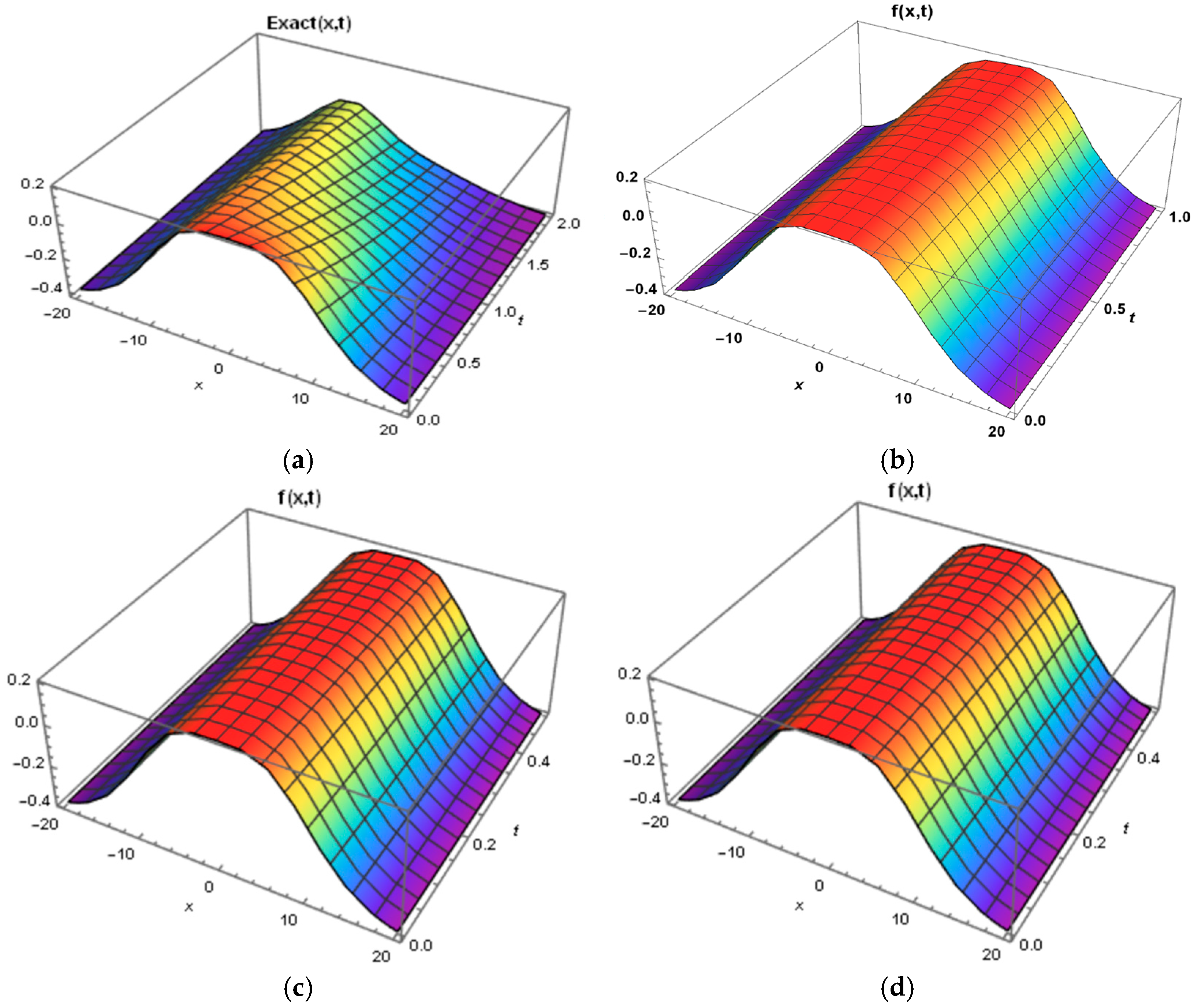
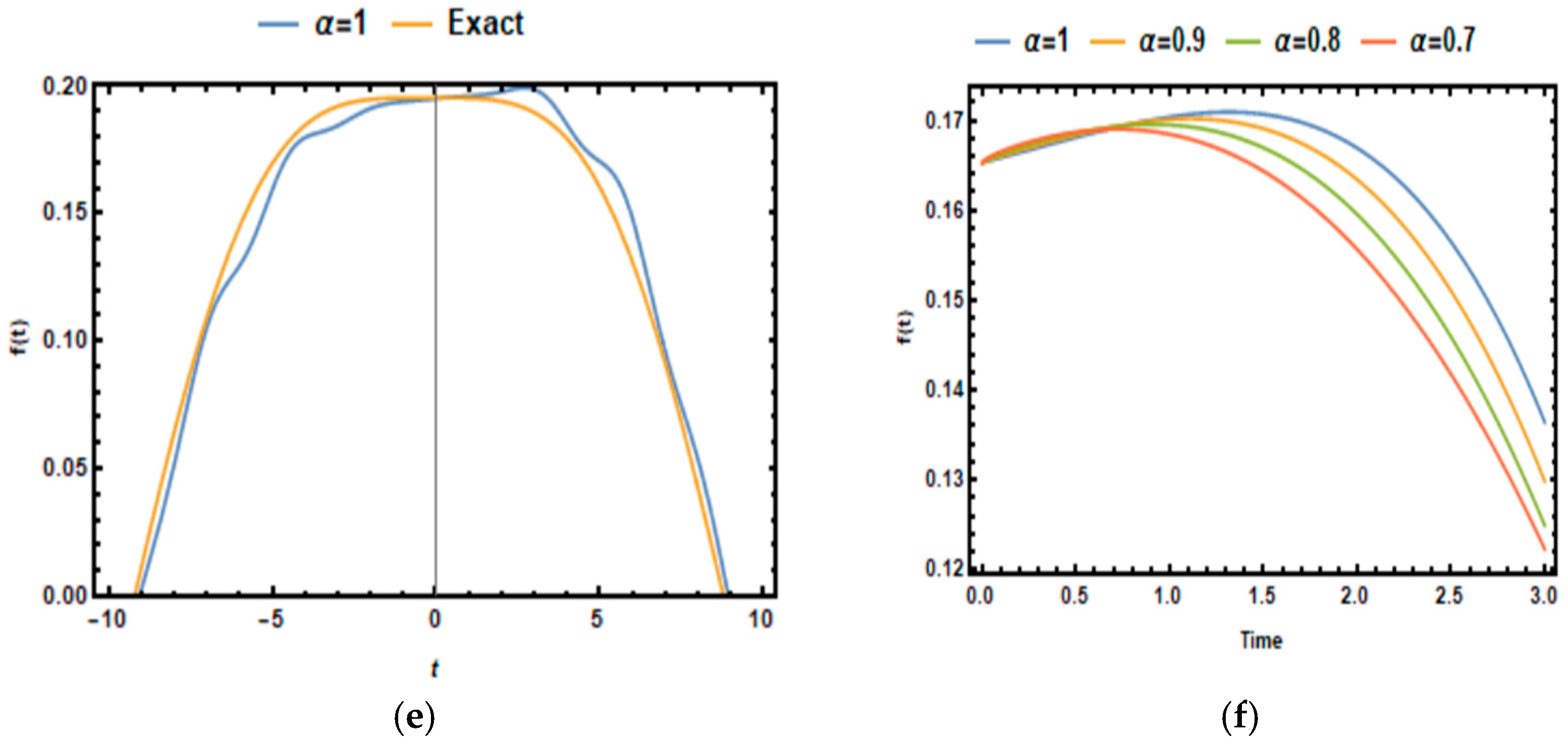
By calculating and summing up the first 15 iteration terms, we were able to obtain a suitable solution and visualize it in Figure 1.

$${ʄ}_n\left(x,t\right)={\sum }_{i=0}^{n=15}{ʄ}_i(x,t)$$

(38)

Also, we derived the absolute error for the different values of $t$ and $x$, as follows:

$$AbsoluteError=\left|\left.F\left(x,t\right)-{ʄ}_n(x,t)\right|\right.$$

(39)

where $F\left(x,t\right)$ is the given exact solution.

We derived the first 15 iteration terms to obtain a suitable solution, and visualized it in Figure 1; the absolute error was also derived in

Table 1. Absolute error when implementing the Kawahara Equations (28) and (29) via the FNIT-HPM, the VIM [34], the HPM [34], and the ADM [35].

x	t	|fexact − fFNIM−HPM|	|fexact − fRSPM|	|fexact − fVIM|	|fexact − fHPM|
−20	0.1	$4.78919\times {10}^{-12}$	7.95296 × 10−10	7.82552 × 10−9	7.95395 × 10−9
	0.2	$4.57886\times {10}^{-11}$	1.61492 × 10−9	1.56394 × 10−8	1.61571 × 10−8
	0.3	$1.79695\times {10}^{-10}$	2.45886 × 10−9	2.34416 × 10−8	2.46153 × 10−8
	0.4	$6.89615\times {10}^{-9}$	3.32711 × 10−9	3.12321 × 10−8	3.33346 × 10−8
	0.5	$1.04554\times {10}^{-9}$	4.21967 × 10−9	3.90108 × 10−8	4.23207 × 10−8
−10	0.1	$3.8441\times {10}^{-11}$	4.53022 × 10−10	4.52809 × 10−9	4.52965 × 10−9
	0.2	$2.76887\times {10}^{-11}$	9.06454 × 10−10	9.05602 × 10−9	9.05996 × 10−9
	0.3	$1.90344\times {10}^{-10}$	1.36030 × 10−9	1.35838 × 10−8	1.35875 × 10−8
	0.4	$5.63816\times {10}^{-9}$	1.81456 × 10−9	1.81115 × 10−8	1.81090 × 10−8
	0.5	1.00256 × 10−9	2.26924 × 10−9	2.26392 × 10−8	2.26209 × 10−8
0	0.1	$5.3306\times {10}^{-15}$	2.00000 × 10−10	2.00000 × 10−10	2.00000 × 10−10
	0.2	$7.1306\times {10}^{-14}$	2.00000 × 10−10	2.00000 × 10−10	2.00000 × 10−10
	0.3	$2.01022\times {10}^{-13}$	1.20000 × 10−9	1.20000 × 10−9	1.20000 × 10−9
	0.4	$6.51022\times {10}^{-12}$	2.90000 × 10−9	2.90000 × 10−9	2.90000 × 10−9
	0.5	$2.22045\times {10}^{-12}$	7.40000 × 10−9	7.40000 × 10−9	7.40000 × 10−9
10	0.1	$3.8441\times {10}^{-11}$	4.52616 × 10−10	4.52828 × 10−9	4.52558 × 10−9
	0.2	$2.76887\times {10}^{-11}$	9.04828 × 10−10	9.05680 × 10−9	9.04371 × 10−9
	0.3	$1.90344\times {10}^{-10}$	1.35664 × 10−9	1.35856 × 10−8	1.35510 × 10−8
	0.4	$5.63816\times {10}^{-9}$	1.80806 × 10−9	1.81146 × 10−8	1.80440 × 10−8
	0.5	1.00256 × 10−9	2.25908 × 10−9	2.26440 × 10−8	2.25193 × 10−8
20	0.1	$4.78919\times {10}^{-12}$	7.70965 × 10−10	7.83709 × 10−9	7.71064 × 10−9
	0.2	$4.57886\times {10}^{-11}$	1.51759 × 10−9	1.56857 × 10−8	1.51839 × 10−8
	0.3	$1.79695\times {10}^{-10}$	2.23988 × 10−9	2.35457 × 10−8	2.24256 × 10−8
	0.4	$6.89615\times {10}^{-9}$	2.93782 × 10−9	3.14172 × 10−8	2.94417 × 10−8
	0.5	$1.04554\times {10}^{-9}$	3.61140 × 10−9	3.92999 × 10−8	3.62381 × 10−8

.

4.2. Case Study 2

Consider the fractional order Kawahara equation is:

$${D_t}^{\alpha }ʄ+ʄ{ʄ}_x+{ʄ}_{3x}-{ʄ}_{5x}=0,$$

(40)

In a simple form with the initial condition:

$$ʄ\left(x,0\right)={\displaystyle \frac{105}{169}}{\mathrm{s}\mathrm{e}\mathrm{c}\mathrm{h}}^4\left(wx\right),$$

(41)

An analytic solution at$\alpha =1$ as follows [33]:

$$ʄ\left(x,t\right)={\displaystyle \frac{105}{169}}{\mathrm{sech}}^4\left(w\left(x+bt\right)\right).$$

(42)

where $w={\displaystyle \frac{1}{2\sqrt{13}}},b={\displaystyle \frac{36}{169}}$.

Start by taking NIT on both sides of Equation (40) we obtain the following:

$$T\left[ʄ\left(x,t\right)\right]=ʄ\left(x,0\right)-{\displaystyle \frac{1}{{ᵴ}^{\alpha }}}T\left[ʄ{ʄ}_x\right]-{\displaystyle \frac{1}{{ᵴ}^{\alpha }}}T\left[{ʄ}_{3x}-{ʄ}_{5x}\right],$$

(43)

Apply the initial condition and take the inverse technique’s effectiveness, as demonstrated through applying the NIT, as follows:

$$ʄ\left(x,t\right)={\displaystyle \frac{105}{169}}{\mathrm{s}\mathrm{e}\mathrm{c}\mathrm{h}}^4[wx]-T^{-1}\left[{\displaystyle \frac{1}{{ᵴ}^{\alpha }}}T\left[ʄ{ʄ}_x\right]\right]-T^{-1}\left[{\displaystyle \frac{1}{{ᵴ}^{\alpha }}}T\left[{ʄ}_{3x}-{ʄ}_{5x}\right]\right],$$

(44)

Now, by substituting He’s polynomials and the HPM concepts on Equation (44), we obtain the following:

$$\begin{gathered} \sum _{n=0}^{\infty }{ϸ}^n{ʄ}_n\left(x,t\right)={\displaystyle \frac{105}{169}}{\mathrm{s}\mathrm{e}\mathrm{c}\mathrm{h}}^4\left[wx\right] \\ -ϸ\left\{T^{-1}\left[{\displaystyle \frac{1}{u}}\left(\begin{array}{c}T\left[{\sum }_{n=0}^{\infty }{ϸ}^n{H}_n\left(ʄ\right)\right]+T\left[{\sum }_{n=0}^{\infty }{ϸ}^n{\left({ʄ}_n\right)}_{3x}\right]\\ -T\left[{\sum }_{n=0}^{\infty }{ϸ}^n{\left({ʄ}_n\right)}_{5x}\right]\end{array}\right)\right]\right\} \end{gathered}$$

(45)

As $H_n\left(ʄ\right)$ represents the non-linear term $ʄ{ʄ}_x$ in Equation (40)

$$H_n\left({ʄ}_0,\dots ,{ʄ}_n\right)=k{\displaystyle \frac{1}{n!}}{\displaystyle \frac{\partial }{\partial {ϸ}^n}}{\left[{\sum }_{i=0}^{\infty }{ϸ}^i{ʄ}_i\left(x,t\right){\left({\sum }_{i=0}^{\infty }{ϸ}^i{ʄ}_i\left(x,t\right)\right)}_x\right]}_{ϸ=0},$$

(46)

where

$$\begin{gathered} H_0\left({ʄ}_0\right)={ʄ}_0{{ʄ}_0}_x, \\ {H}_1\left({ʄ}_0,{ʄ}_1\right)={ʄ}_1{{ʄ}_0}_x+{ʄ}_0{{ʄ}_1}_x, \\ ⋮ \\ ⋮ \\ {H}_n\left({ʄ}_0,\dots ,{ʄ}_n\right)={ʄ}_n{{ʄ}_0}_x+{ʄ}_{n-1}{{ʄ}_1}_x+\dots +{ʄ}_1{{ʄ}_{n-1}}_x+{ʄ}_0{{ʄ}_n}_x, \end{gathered}$$

(47)

So, by equating the coefficients of p with the same powers in (45), it leads to the following:

$$\begin{gathered} {ϸ}^0:{ʄ}_0\left(x,t\right)={\displaystyle \frac{105}{169}}({\mathit{sech}}^{4}wx) \\ {ϸ}^1:{ʄ}_1\left(x,t\right)=-T^{-1}\left[{\displaystyle \frac{1}{{ᵴ}^{\alpha }}}\left(\begin{array}{c}T\left[H_0\left(x,t\right)\right]+T\left[{\left({ʄ}_0\right)}_{3x}\right]\\ -T\left[{\left({ʄ}_0\right)}_{5x}\right]\end{array}\right)\right] \\ ={\displaystyle \frac{7560t^{\alpha }{sech}^4[\frac{x}{2\sqrt{13}}]\mathit{tanh}[\frac{x}{2\sqrt{13}}]}{28561\sqrt{13}\Gamma [1+\alpha ]}} \\ {ϸ}^2:{ʄ}_2\left(x,t\right)={\displaystyle \frac{136080t^{2\alpha }(-3+2\mathit{cosh}[\frac{x}{\sqrt{13}}]){sech[\frac{x}{2\sqrt{13}}]}^6}{62748517\Gamma [1+2\alpha ]}}, \\ {ϸ}^3:{ʄ}_3\left(x,t\right)=((204120t^{3\alpha }((765-650\mathit{cosh}\left[{\displaystyle \frac{x}{\sqrt{13}}}\right]-9\mathit{cosh}\left[{\displaystyle \frac{x}{\sqrt{13}}}\right]+6\mathit{cosh}[{\displaystyle \frac{x}{\sqrt{13}}}]){\begin{array}{c}\\ \Gamma \left[1+\alpha \right]\end{array}}^2+140\left(-3+2\mathit{cosh}[{\displaystyle \frac{x}{\sqrt{13}}}]\right)\Gamma [1+2\alpha ]){sech[{\displaystyle \frac{x}{2\sqrt{13}}}]}^{10} \\ \mathit{tanh}[{\displaystyle \frac{x}{2\sqrt{13}}}])/\left(10604499373\sqrt{13}{\Gamma \left[1+\alpha \right]}^2\Gamma \right[1+3\alpha \left]\right)) \end{gathered}$$

(48)

Similarly, the values of ${ʄ}_4\left(x,t\right)$; ${ʄ}_5\left(x,t\right)$;…. can be obtained.

Finally, the approximated solution is the summation of all components of the previous series in Equation (48) as follows:

$$ʄ\left(x,t\right)={ʄ}_0\left(x,t\right)+{ʄ}_1\left(x,t\right)+{ʄ}_2\left(x,t\right)+{ʄ}_3\left(x,t\right)+\dots .$$

(49)

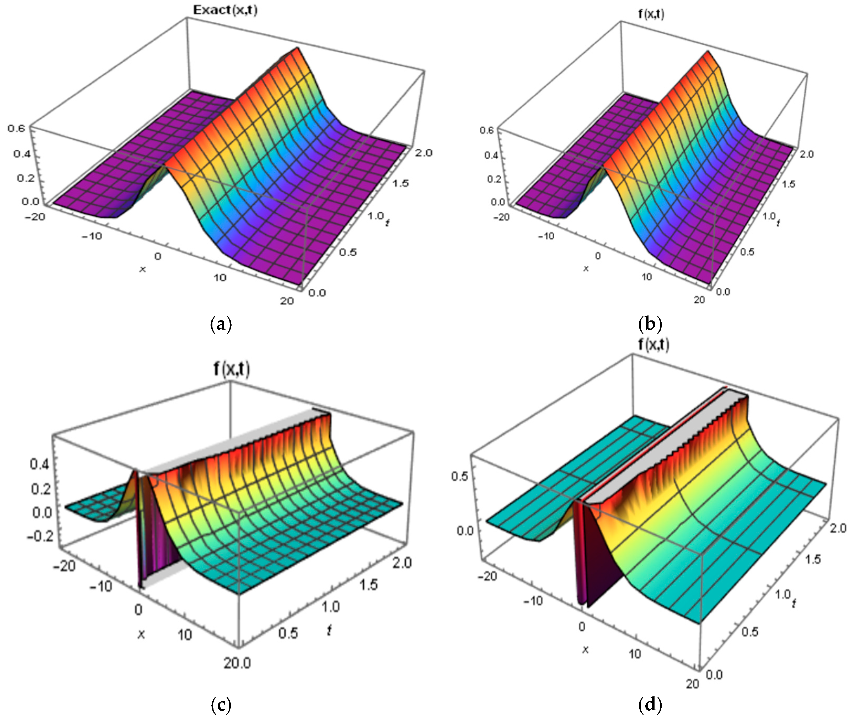
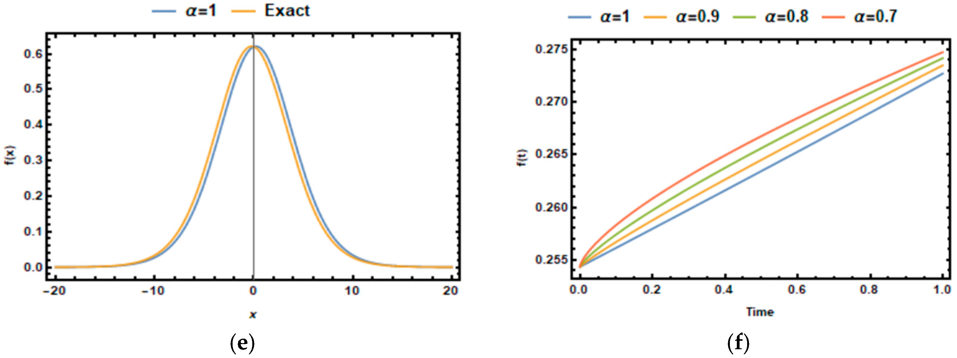
As with the previous application, we derived the first 15 iteration terms to obtain a suitable solution and visualized it in Figure 2; the absolute error was also derived in

Table 2. Absolute error of applications (40) and (41) by the FNIT-HPM, the VIM [34], the HPM [34], and the ADM methods [35].

x	t	|fexact − fFNIM−HPM|	|fexact − frspm|	|fexact − fVIM|	|fexact − fHPM|
−20	0.1	$3.48919\times {10}^{-12}$	1.58361 × 10−11	3.97274 × 10−11	1.01469 × 10−8
	0.2	$6.97886\times {10}^{-12}$	8.28473 × 10−11	3.13089 × 10−10	4.04332 × 10−8
	0.3	$1.04695\times {10}^{-11}$	5.38679 × 10−10	1.05406 × 10−9	9.06246 × 10−8
	0.4	$1.39615\times {10}^{-10}$	2.82485 × 10−9	2.49070 × 10−9	1.60493 × 10−7
	0.5	$1.74554\times {10}^{-10}$	7.28460 × 10−9	4.85110 × 10−9	2.49809 × 10−7
−10	0.1	$6.3441\times {10}^{-11}$	8.29485 × 10−10	2.46593 × 10−9	1.53191 × 10−6
	0.2	$1.26887\times {10}^{-10}$	4.83572 × 10−9	1.92434 × 10−8	6.11064 × 10−6
	0.3	$1.90344\times {10}^{-9}$	1.63892 × 10−8	6.48336 × 10−8	1.37103 × 10−5
	0.4	$2.53816\times {10}^{-9}$	7.04823 × 10−8	1.53132 × 10−7	2.43056 × 10−5
	0.5	6.90256 × 10−8	3.47678 × 10−7	2.98332 × 10−7	3.78709 × 10−5
0	0.1	$3.3306\times {10}^{-16}$	2.00732 × 10−10	1.74165 × 10−10	5.42153 × 10−6
	0.2	$0$	8.48329 × 10−10	1.77754 × 10−9	2.16847 × 10−5
	0.3	$1.11022\times {10}^{-16}$	3.18473 × 10−9	9.03168 × 10−9	4.87858 × 10−5
	0.4	$1.11022\times {10}^{-16}$	9.48372 × 10−9	2.82581 × 10−8	8.67179 × 10−5
	0.5	$2.22045\times {10}^{-16}$	4.03846 × 10−8	6.90256 × 10−8	1.35472 × 10−4
10	0.1	$6.3441\times {10}^{-11}$	6.03826 × 10−10	2.41376 × 10−9	1.54059 × 10−6
	0.2	$1.26887\times {10}^{-10}$	2.94573 × 10−9	1.94624 × 10−8	6.17975 × 10−6
	0.3	$1.90344\times {10}^{-9}$	9.89347 × 10−9	6.58172 × 10−8	1.39436 × 10−5
	0.4	$2.53816\times {10}^{-9}$	4.28345 × 10−8	1.56456 × 10−7	2.48584 × 10−5
	0.5	6.90256 × 10−8	1.38277 × 10−7	3.06352 × 10−7	3.89507 × 10−5
20	0.1	$3.48919\times {10}^{-12}$	2.28467 × 10−11	3.98825 × 10−11	1.02266 × 10−8
	0.2	$6.97886\times {10}^{-12}$	8.68913 × 10−11	3.16631 × 10−10	4.10637 × 10−8
	0.3	$1.04695\times {10}^{-11}$	5.03682 × 10−10	1.07259 × 10−9	9.27540 × 10−8
	0.4	$1.39615\times {10}^{-10}$	2.00384 × 10−9	2.54866 × 10−9	1.65539 × 10−7
	0.5	$1.74554\times {10}^{-10}$	7.28395 × 10−9	4.99298 × 10−9	2.59666 × 10−7

.

The accuracy of the FNIT-HPM method is assessed by calculating absolute errors, as presented in Table 2. These errors represent the difference between the exact solution and the approximated values at various points. The results indicate that the proposed method produces highly precise solutions, showing significantly lower error values compared to other approaches, such as the VIM, the HPM, and the ADM.

From the data, we observe that the error remains minimal for smaller values of $t$, suggesting that the FNIT-HPM method converges quickly in the early stages. As $t$ increases, a slight rise in error is noted, which is expected due to the accumulation of small numerical approximations over iterations. However, the error remains well within acceptable limits, demonstrating the robustness of the method.

Additionally, the nature of the Kawahara equation, particularly the presence of higher-order derivatives, influences the observed error patterns. Nonlinear terms tend to introduce numerical sensitivity, which can impact the precision of traditional methods. By leveraging its integral transform properties, the FNIT-HPM approach effectively reduces these errors and enhances stability.

This evaluation confirms that the FNIT-HPM is a reliable and efficient tool for solving fractional nonlinear differential equations, maintaining accuracy while improving computational efficiency.

5. Homogeneous Form of Fractional Coupled Burgers’ Equations

Now consider the solution of the homogeneous form of the coupled Burgers’ equations:

$$\left\{\begin{array}{c}{D_t}^{\alpha }ʄ-{ʄ}_{2x}-ʄ{ʄ}_x-{(ʄɠ)}_x=0,\\ {D_t}^{\alpha }ɠ-{ɠ}_{2x}-ɠ{ɠ}_x-{(ʄɠ)}_x=0\end{array}\right..$$

(50)

With the initial condition:

$$\left\{\begin{array}{c}ʄ\left(x,0\right)=\mathrm{c}\mathrm{o}\mathrm{s}\left(x\right),\\ ɠ\left(x,0\right)=\mathrm{c}\mathrm{o}\mathrm{s}\left(x\right),\end{array}\right..$$

(51)

Which has an analytic solution as follows [28]:

$$ʄ\left(x,t\right)=ɠ\left(x,t\right)=e^{-t}\mathrm{c}\mathrm{o}\mathrm{s}\left(x\right)$$

(52)

Assume that the solutions of Equation (50) can be written as a power series as follows:

$$\left\{\begin{array}{c}ʄ\left(x,t\right)=\sum _{n=0}^{\infty }{ϸ}^n{ʄ}_n\left(x,t\right),\\ ɠ\left(x,t\right)=\sum _{n=0}^{\infty }{ϸ}^n{ɠ}_n\left(x,t\right),\end{array}\right.$$

(53)

As illustrated in case study 1, start by taking FNIT on both sides of Equation (50) we obtain the following:

$$\left\{\begin{array}{c}T\left[ʄ\left(x,t\right)\right]=ʄ\left(x,0\right)-{\displaystyle \frac{1}{{ᵴ}^{\alpha }}}[T\left[{ʄ}_{2x}+ʄ{ʄ}_x+{(ʄɠ)}_x\right]],\\ T\left[ɠ\left(x,t\right)\right]=ɠ\left(x,0\right)-{\displaystyle \frac{1}{{ᵴ}^{\alpha }}}[T\left[{ɠ}_{2x}+ɠ{ɠ}_x+{(ʄɠ)}_x\right]],\end{array}\right.$$

(54)

Next, apply the initial condition and take the inverse of the FNIT:

$$ʄ\left(x,t\right)=\mathrm{c}\mathrm{o}\mathrm{s}(x)-T^{-1}\left[{\displaystyle \frac{1}{{ᵴ}^{\alpha }}}T\left[{ʄ}_{2x}\right]\right]-T^{-1}\left[{\displaystyle \frac{1}{{ᵴ}^{\alpha }}}T\left[ʄ{ʄ}_x+{(ʄɠ)}_x\right]\right],$$

(55)

Now, by substituting He’s polynomials and the HPM concepts in Equation (53), we obtain the following:

$$\left\{\begin{array}{c}{\displaystyle \sum _{n=0}^{\infty }}{ϸ}^n{ʄ}_n\left(x,t\right)=T^{-1}\left\{\cos \left(x\right)\right\}+ϸ\left\{T^{-1}\left[{\displaystyle \frac{1}{{ᵴ}^{\alpha }}}\left(\begin{array}{c}T\left[{\displaystyle \sum _{n=0}^{\infty }}{ϸ}^n{H}_n\left(ʄ\right)\right]+T\left[{\displaystyle \sum _{n=0}^{\infty }}{ϸ}^n{\left({ʄ}_n\right)}_{2x}\right]\\ +T\left[{\displaystyle \sum _{n=0}^{\infty }}{ϸ}^n\left({ʄ}_n{\left({ʄ}_n\right)}_x\right)\right]+T\left[{\displaystyle \sum _{n=0}^{\infty }}{ϸ}^n{\left({ʄ}_n{ɠ}_n\right)}_x\right]\end{array}\right)\right]\right\}\\ {\displaystyle \sum _{n=0}^{\infty }}{ϸ}^n{ɠ}_n\left(x,t\right)=T^{-1}\left\{\cos \left(x\right)\right\}+ϸ\left\{T^{-1}\left[{\displaystyle \frac{1}{{ᵴ}^{\alpha }}}\left(\begin{array}{c}T\left[{\displaystyle \sum _{n=0}^{\infty }}{ϸ}^n{H}_n\left(ɠ\right)\right]+T\left[{\displaystyle \sum _{n=0}^{\infty }}{ϸ}^n{\left({ɠ}_n\right)}_{2x}\right]\\ +T\left[{\displaystyle \sum _{n=0}^{\infty }}{ϸ}^n\left({ɠ}_n{\left({ɠ}_n\right)}_x\right)\right]+T\left[{\displaystyle \sum _{n=0}^{\infty }}{ϸ}^n{\left({ʄ}_n{ɠ}_n\right)}_x\right]\end{array}\right)\right]\right\}.\end{array}\right.$$

(56)

As $H_n\left(ʄ\right)$ represents He’s polynomials of the non-linear part ${ʄʄ}_x$, ${ɠɠ}_x$, ${(ʄɠ)}_x$ in Equation (56):

$$H_n\left({ʄ}_0,...,{ʄ}_n\right)={\displaystyle \frac{1}{n!}}{\displaystyle \frac{\partial }{\partial {ϸ}^n}}{\left[\left({\sum }_{i=0}^{\infty }{ϸ}^i{ʄ}_i\left(x,t\right)\right){\left({\sum }_{i=0}^{\infty }{ϸ}^i{ʄ}_i\left(x,t\right)\right)}_x\right]}_{ϸ=0},$$

(57)

So, by equating the coefficients of p with the same powers in (56) leads to the following:

$$\begin{gathered} {ϸ}^0:\left\{\begin{array}{c}{ʄ}_0\left(x,t\right)=T^{-1}\left\{\mathrm{c}\mathrm{o}\mathrm{s}\left(x\right)\right\}=\cos \left(x\right),\\ {ɠ}_0\left(x,t\right)=T^{-1}\left\{\mathrm{c}\mathrm{o}\mathrm{s}\left(x\right)\right\}=\cos \left(x\right),\end{array}\right. \\ {ϸ}^1:\left\{\begin{array}{c}{ʄ}_1\left(x,t\right)=T^{-1}\left[{\displaystyle \frac{1}{{ᵴ}^{\alpha }}}\left\{T\left[2{ʄ}_0{ʄ}_{0x}-{ɠ}_0{ʄ}_{0x}-{ʄ}_0{ɠ}_{0x}+{\left({ʄ}_0\right)}_{2x}\right]\right\}\right]=T^{-1}\left[-{\displaystyle \frac{1}{ᵴ}}cos(x)\right],\\ {ɠ}_1\left(x,t\right)=T^{-1}\left[{\displaystyle \frac{1}{{ᵴ}^{\alpha }}}\left\{T\left[2{ɠ}_0{ɠ}_{0x}-{ʄ}_0{ɠ}_{0x}-{ɠ}_0{ɠ}_{0x}+{\left({ɠ}_0\right)}_{2x}\right]\right\}\right]=T^{-1}\left[-{\displaystyle \frac{1}{ᵴ}}cos(x)\right],\end{array}\right. \\ {ϸ}^2:\left\{\begin{array}{c}{ʄ}_2\left(x,t\right)=T^{-1}\left[{\displaystyle \frac{1}{{ᵴ}^{\alpha }}}\left\{T\left[2{ʄ}_1{ʄ}_{0x}-{ɠ}_1{ʄ}_{0x}+2{ʄ}_0{ɠ}_{1x}-{ɠ}_0{ʄ}_{1x}-{ʄ}_1{ɠ}_{0x}-{ʄ}_0{ɠ}_{1x}+{\left({ʄ}_1\right)}_{2x}\right]\right\}\right],\\ {ɠ}_2\left(x,t\right)=T^{-1}\left[{\displaystyle \frac{1}{{ᵴ}^{\alpha }}}\left\{T\left[2{ɠ}_1{ɠ}_{0x}-{ʄ}_1{ɠ}_{0x}+2{ɠ}_0{ʄ}_{1x}-{ʄ}_0{ɠ}_{1x}-{ɠ}_1{ɠ}_{0x}-{ɠ}_0{ʄ}_{1x}+{\left({ɠ}_1\right)}_{2x}\right]\right\}\right],\end{array}\right. \\ {ϸ}^3:\left\{\begin{array}{c}{ʄ}_3\left(x,t\right)=T^{-1}\left[{\displaystyle \frac{1}{{ᵴ}^{\alpha }}}\left\{T\left[\begin{array}{c}2{ʄ}_2{ʄ}_{0x}-{ɠ}_2{ʄ}_{0x}+2{ʄ}_1{ʄ}_{1x}-{ɠ}_1{ʄ}_{1x}+2{ʄ}_0{ʄ}_{2x}\\ -{ɠ}_0{ɠ}_{2x}-{ʄ}_2{ʄ}_{0x}-{ʄ}_1{ɠ}_{2x}-{ʄ}_0{ɠ}_{2x}+{\left({ʄ}_2\right)}_{2x}\end{array}\right]\right\}\right],\\ {ɠ}_3\left(x,t\right)=T^{-1}\left[{\displaystyle \frac{1}{{ᵴ}^{\alpha }}}\left\{T\left[\begin{array}{c}2{ɠ}_2{ɠ}_{0x}-{ʄ}_2{ɠ}_{0x}+2{ɠ}_1{ɠ}_{1x}-{ʄ}_1{ɠ}_{1x}+2{ɠ}_0{ɠ}_{2x}\\ -{ʄ}_0{ʄ}_{2x}-{ɠ}_2{ɠ}_{0x}-{ɠ}_1{ʄ}_{2x}-{ɠ}_0{ʄ}_{2x}+{\left({ɠ}_2\right)}_{2x}\end{array}\right]\right\}\right],\end{array}\right. \end{gathered}$$

(58)

Finally, the approximated solution is the summation of all components of the previous series in Equation (58) as follows:

$$\left\{\begin{array}{c}ʄ\left(x,t\right)={ʄ}_0\left(x,t\right)+{ʄ}_1\left(x,t\right)+{ʄ}_2\left(x,t\right)+{ʄ}_3\left(x,t\right)+\dots .\\ ʄ\left(x,t\right)={ɠ}_0\left(x,t\right)+{ɠ}_1\left(x,t\right)+{ɠ}_2\left(x,t\right)+{ɠ}_3\left(x,t\right)+\dots .\end{array}\right.$$

(59)

As with the previous application, we derived the first 15 iteration terms, to obtain a suitable solution and visualized it in Figure 3.

$$\left\{\begin{array}{c}ʄ\left(x,t\right)=\mathit{cos}\left(x\right)\left[1-t+{\displaystyle \frac{t^2}{2!}}-{\displaystyle \frac{t^3}{3!}}+{\displaystyle \frac{t^4}{4!}}\right]=e^{-t}\mathit{cos}\left(x\right),\\ ɠ\left(x,t\right)=\mathit{cos}\left(x\right)\left[1-t+{\displaystyle \frac{t^2}{2!}}-{\displaystyle \frac{t^3}{3!}}+{\displaystyle \frac{t^4}{4!}}\right]=e^{-t}\mathit{cos}\left(x\right),\end{array}\right.$$

(60)

6. Discussion

This study focuses on solving fractional partial differential equations, particularly the modified Kawahara equation and the coupled Burgers’ equation, utilizing fractional derivatives in the Caputo sense. To achieve this, we introduce the fractional new integral transform–homotopy perturbation method (FNIT-HPM), an innovative approach that effectively integrates the new integral transform with the homotopy perturbation method. This hybrid technique establishes a structured and computationally efficient framework for deriving approximate analytical solutions to nonlinear fractional differential equations. The FNIT facilitates the simplification of complex differential operators, while the HPM ensures rapid convergence without the need for perturbation assumptions or linearization.

To evaluate its performance, the FNIT-HPM is applied to two case studies for the modified Kawahara equation and the homogeneous coupled Burgers’ equations, both formulated with Caputo fractional derivatives. These equations play a critical role in modeling nonlinear wave phenomena and fluid dynamics. The approximate solutions obtained using the FNIT-HPM have been contrasted with exact solutions and outcomes from established numerical techniques, including the variational iteration method (VIM), the homotopy perturbation method (HPM) alone, and the Adomian decomposition method (ADM). Numerical tables and graphical representations of error analysis indicate that the FNIT-HPM outperforms the existing methods in terms of accuracy and convergence speed. The reported absolute errors, particularly for small values of $x$ and $t$, reach as low as ${10}^{-12}$, demonstrating the method’s superior precision and reliability for solving fractional differential equations.

A key advantage of the FNIT-HPM is its ability to handle fractional-order differentiation, making it highly effective for physical models that exhibit memory effects and anomalous diffusion. As shown in Figure 1 and Figure 2, the approximate solutions closely align with exact solutions, especially as the fractional order parameter β approaches one. This demonstrates the versatility of the FNIT-HPM for solving time–fractional nonlinear wave equations, as well as its capacity to simulate complex physical processes that are not covered by classic integer-order differential equations.

Additionally, the successful application of the FNIT-HPM to coupled Burgers’ equations highlights its potential for addressing nonlinear coupled systems with fractional derivatives.

The efficiency of the FNIT-HPM lies in its synergistic integration of the FNIT with the homotopy perturbation approach. By simplifying the governing equations before applying perturbation techniques, the FNIT minimizes the computational burden associated with complex numerical calculations. Unlike conventional numerical methods that rely on discretization or iterative schemes prone to instability, the FNIT-HPM produces highly accurate approximations with fewer iterations and reduced computational effort.

In conclusion, the FNIT-HPM offers a powerful mathematical framework for solving nonlinear fractional partial differential equations in the Caputo sense. Its applications extend to wave propagation, fluid mechanics, and nonlinear dynamics, where high accuracy, fast convergence, and computational efficiency are essential. Given its advantages over traditional techniques, the FNIT-HPM stands as a promising alternative for fractional differential equation modeling. Future research could extend this approach to higher dimensional fractional systems, nonlinear Schrödinger equations, and chaotic fractional-order models, further solidifying its relevance in applied mathematical modeling.

7. Conclusions

This research presents an enhanced variant of the homotopy perturbation method (HPM), achieved by incorporating a novel integral transform. The proposed approach facilitates exact solutions for the Kawahara equation and nonlinear coupled systems when the derivative order is an integer $(\alpha =1$), while also yielding approximate solutions for fractional-order derivatives. The accuracy and efficiency of the FNIT-HPM method were assessed through various examples, illustrating its effectiveness in approximating both linear and nonlinear differential equations. By integrating the new integral transform with the HPM within the framework of Caputo fractional derivatives, we establish a reliable and efficient numerical methodology for handling partial differential equations, both independently and within system-based contexts.

The proposed methodology utilizes the FNIT-HPM to transform partial differential equations into a system of ordinary differential equations. This technique produces numerical results that closely align with established analytical and benchmark solutions. A comparative assessment reveals that the introduced approach outperforms conventional numerical methods in both accuracy and computational efficiency, positioning it as a promising alternative for tackling complex nonlinear partial differential equations.

The integration of the new integral transform (NIT) with the HPM under the Caputo fractional derivative framework enhances the precision and robustness of the proposed numerical method. By converting partial differential equations into a solvable set of ordinary differential equations and applying the HPM for iterative approximations, the numerical results closely align with established analytical solutions. Given its superior performance over conventional numerical techniques, the FNIT-HPM presents itself as a useful and promising option for tackling nonlinear fractional partial differential equations. In future studies, the FNIT-HPM approach could be used in more complex systems, such as higher-dimensional and multivariable partial differential equations. Furthermore, incorporating machine learning techniques into the FNIT-HPM may increase its flexibility and effectiveness in tackling a wider range of nonlinear issues. Further research could look into the practical use of the FNIT-HPM in real-world engineering and physics contexts, providing more insight into its possible applications.