A Fractional Time–Space Stochastic Advection–Diffusion Equation for Modeling Atmospheric Moisture Transport at Ocean–Atmosphere Interfaces

Abstract

This study introduces a novel one-dimensional Fractional Time–Space Stochastic Advection–Diffusion Equation that revolutionizes the modeling of moisture transport within atmospheric boundary layers adjacent to oceanic surfaces. By synthesizing fractional calculus, advective transport mechanisms, and pink noise stochasticity, the proposed model captures the intricate interplay between temporal memory effects, non-local turbulent diffusion, and the correlated-fluctuations characteristic of complex ocean–atmosphere interactions. The framework employs the Caputo fractional derivative to represent temporal persistence and the fractional Laplacian to model non-local turbulent diffusion, and incorporates a stochastic term with a $1/f$ power spectral density to simulate environmental variability. An efficient numerical solution methodology is derived utilizing complementary Fourier and Laplace transforms, which elegantly converts spatial fractional operators into algebraic expressions and yields closed-form solutions via Mittag–Leffler functions. This method’s application to a benchmark coastal domain demonstrates that stronger advection significantly increases the spatial extent of conditions exceeding fog formation thresholds, revealing advection’s critical role in moisture transport dynamics. Numerical simulations demonstrate the model’s capacity to reproduce both anomalous diffusion phenomena and realistic stochastic variability, while convergence analysis confirms the numerical scheme’s robustness against varying noise intensities. This integrated fractional stochastic framework substantially advances atmospheric moisture modeling capabilities, with direct applications to meteorological forecasting, coastal climate assessment, and environmental engineering.

1. Introduction

The Advection–Diffusion Equation (ADE) stands as a cornerstone mathematical framework that elegantly describes the transport phenomena of substances in fluid flows. This powerful equation captures the dual physical processes of advection—the transport of materials by bulk fluid motion—and diffusion—the spreading of particles due to random molecular movements [1,2]. Its versatility and broad applicability have made it indispensable across numerous scientific and engineering disciplines.

In environmental engineering, the ADE serves as the foundation for modeling pollutant dispersion in atmospheric and aquatic systems. Researchers have developed sophisticated analytical solutions using methods like separation of variables and the Generalized Integral Laplace Transform Technique (GILTT) to simulate how contaminants spread through different environmental media [3]. These models prove crucial for predicting air quality, assessing water pollution, and designing effective remediation strategies.

The equation’s utility extends deeply into fluid dynamics, where it illuminates complex processes such as sediment transport in rivers and coastal environments. Stochastic interpretations of the ADE have enhanced our understanding of the statistical properties of particle movement in these systems [4], providing valuable insights for river management and coastal protection initiatives.

Hydrogeologists rely on the ADE to track contaminant migration through groundwater systems, while chemical engineers apply it to optimize reaction processes in industrial settings [5]. The medical field has adopted variants of the equation to model drug delivery and distribution within biological systems.

Recent mathematical innovations have expanded the ADE’s applicability to scenarios involving time-dependent velocity fields and anisotropic diffusion [6]. Numerical methods like the Du-Fort–Frankel approach have enabled solutions to real-world problems in irregular domains that were previously intractable [7]. These advancements continue to broaden the equation’s reach across scientific disciplines.

The ADE thus represents not merely a mathematical construct but a powerful conceptual tool that bridges theoretical understanding and practical application across the natural and engineered worlds [8], demonstrating the profound unity underlying seemingly disparate physical phenomena.

The ADE is a fundamental mathematical model used extensively in environmental engineering to describe the transport and dispersion of substances within various media. In water bodies, it models the spread of pollutants such as dissolved salts, chemicals, and bacteria in rivers, lakes, and coastal environments, with applications including the simulation of pollutant propagation in Guaíba Lake, Brazil, to assist local water treatment and sewage disposal authorities [9,10,11]. For groundwater systems, the equation is essential for understanding the movement of contaminants like phosphorus and other solutes through aquifers, where its nonlinear variant, Richard’s equation, proves particularly valuable for simulating water content in unsaturated porous media [12,13,14]. In air pollution modeling, the ADE predicts the dispersion of atmospheric pollutants, aiding in the assessment of industrial emissions and natural disaster impacts on air quality, with techniques like the Advection–Diffusion Multilayer Method (ADMM) offering accurate semi-analytical solutions [15]. The equation also supports soil contamination studies by modeling the movement of contaminants through soil, including non-classical phenomena like superdiffusion, which informs effective remediation strategies [13]. In hydrology, it facilitates the modeling of water transfer and tracer spread in water bodies, notably in the study of high-velocity pollutant transport in heterogeneous aquifers [16]. Additionally, the ADE contributes to the design and operation of sedimentation basins and hindered-settling columns for separating contaminants from soil, enhancing soil classification and remediation efforts [17,18]. Finally, the development of numerical and analytical solutions, such as the lattice Boltzmann method and the Generalized Integral Transform Technique (GITT), enables the ADE to address complex environmental systems, providing critical validation for transport models and optimizing engineering processes [13,19]. These diverse applications highlight the ADE’s versatility and its critical role in tackling environmental engineering challenges. The modeling of complex transport phenomena has been significantly advanced by recent developments in fractional stochastic partial differential equations (PDEs), as comprehensively reviewed by Moghaddam et al. [20]. Their state-of-the-art survey explores numerical techniques and practical applications of fractional stochastic PDEs, emphasizing their ability to capture anomalous diffusion and randomness in systems with symmetry-breaking characteristics. This work underscores the growing importance of integrating fractional calculus with stochastic processes, providing a robust foundation for addressing real-world challenges in diverse fields such as environmental modeling and geophysical dynamics. Building on these insights, our study extends the application of such frameworks to atmospheric moisture transport at ocean–atmosphere interfaces, introducing a novel Fractional Time–Space Stochastic Advection–Diffusion equation tailored to this context.

Our research introduces a novel one-dimensional Fractional Time–Space Stochastic Advection–Diffusion Equation (FTSADE) that characterizes moisture transport processes within an atmospheric layer adjacent to oceanic surfaces. This mathematical framework delineates specific humidity variations along a horizontal transect, employing fractional calculus principles, advective transport mechanisms, and pink noise stochasticity to represent the sophisticated interplay between temporal memory effects, turbulent phenomena, and random fluctuations arising from ocean–atmosphere coupling.

The governing equation adopts an “Atmospheric Moisture Transport” paradigm, with each mathematical component corresponding to a distinct physical mechanism:

$$\underset{\begin{array}{c}\mathrm{Memory}\mathrm{Effects}\\ (\mathrm{Temporal}\mathrm{Persistence})\end{array}}{\underbrace{{}^c\mathit{\partial }_t^{\alpha }q(x,t)}}+\underset{\begin{array}{c}\mathrm{Maritime}\text{-}\mathrm{Induced}\\ \mathrm{Turbulent}\mathrm{Mixing}\end{array}}{\underbrace{{\kappa }_{\beta }{(-\Delta )}^{\beta /2}q(x,t)}}+\underset{\begin{array}{c}\mathrm{Advection}\mathrm{by}\\ \mathrm{Marine}\mathrm{Winds}\end{array}}{\underbrace{v{\displaystyle \frac{\mathit{\partial }q(x,t)}{\mathit{\partial }x}}}}=\underset{\begin{array}{c}\mathrm{Correlated}\mathrm{Noise}\\ (\mathrm{Ocean}\text{-}\mathrm{Air}\mathrm{Interface})\end{array}}{\underbrace{\sigma \eta (x,t).}}$$

(1)

The specific humidity function $q(x,t)$ is defined over the spatial domain $x\in [c,c+L]$ and temporal domain $t>0$, with fractional parameter constraints $0<\alpha \le 1$ and $0<\beta \le 2$.

The model incorporates boundary specifications through the initial condition $q(x,0)=q_0\left(x\right)$ for $x\in [c,c+L]$ and periodic boundary condition $q(c,t)=q(c+L,t)$, which encapsulates the cyclical nature of moisture exchange processes.

Each term in Equation (1) represents distinct physical phenomena. The Caputo fractional temporal derivative term ${}^c\mathit{\partial }_t^{\alpha }q$ captures moisture memory effects through temporal persistence. The fractional Laplacian term ${\kappa }_{\beta }{(-\Delta )}^{\beta /2}q$ represents non-local turbulent diffusion processes driven by oceanic influences. The advection term $v{\displaystyle \frac{\mathit{\partial }q}{\mathit{\partial }x}}$ accounts for directional moisture transport by marine winds with velocity v measured in m/s. The stochastic forcing term $\sigma \eta (x,t)$ introduces correlated fluctuations at the ocean–air interface.

The model employs several physically meaningful parameters. The specific humidity $q(x,t)$, measured in kg/kg, represents the mass ratio of water vapor to total air mass—a dimensionless metric particularly appropriate for atmospheric moisture content characterization, as it remains invariant to changes in pressure and temperature commonly experienced in oceanic boundary layers. This formulation provides advantages over volumetric concentration measures (kg/m³) by ensuring consistency across vertical atmospheric profiles.

The diffusivity coefficient ${\kappa }_{\beta }$ quantifies turbulent dispersion rates along the horizontal domain. The fractional diffusion exponent $\beta$ modulates diffusion behavior: values approaching zero indicate super-diffusive regimes characterized by rapid mixing, while values near 2 correspond to sub-diffusive processes with hindered spreading rates. Wind velocity v represents the mean horizontal air motion driving advective transport. The noise amplitude $\sigma$ scales the correlated stochastic perturbations $\eta (x,t)$, which exhibit power spectral density proportional to $1/f$, capturing temporally coherent moisture fluctuations.

This one-dimensional framework successfully integrates fractional diffusion mechanics, advective transport, and correlated stochastic processes, with $q(x,t)$, measured in kg/kg, providing a robust representation of moisture dynamics in oceanic atmospheric contexts.

The Caputo fractional derivative is mathematically expressed as

$$\underset{\begin{array}{c}\mathrm{Memory}\mathrm{Effects}\\ (\mathrm{Temporal}\mathrm{Persistence})\end{array}}{\underbrace{{}^c\mathit{\partial }_t^{\alpha }q(x,t)}}={\displaystyle \frac{1}{\Gamma (1-\alpha )}}{\int }_0^t{\displaystyle \frac{\mathit{\partial }q(x,\tau )}{\mathit{\partial }\tau }}{\displaystyle \frac{1}{{(t-\tau )}^{\alpha }}}d\tau ,0<\alpha <1.$$

(2)

This integral formulation encapsulates temporal memory by applying diminishing weights to historical system states, effectively modeling the gradual dissipation of moisture memory in turbulent atmospheric conditions.

The one-dimensional fractional Laplacian operator is defined through

$$\underset{\begin{array}{c}\mathrm{Maritime}\text{-}\mathrm{Induced}\\ \mathrm{Turbulent}\mathrm{Mixing}\end{array}}{\underbrace{{\kappa }_{\beta }{(-\Delta )}^{\beta /2}q(x,t)}}={\kappa }_{\beta }\left(-{\displaystyle \frac{1}{2cos(\pi \beta /2)}}\left({}_{c}D_x^{\beta }q(x,t)+{}_{x}D_{c+L}^{\beta }q(x,t)\right)\right),$$

(3)

where the Riemann–Liouville fractional derivatives are given by

$$\begin{array}{cc}\hfill {}_{c}D_x^{\beta }q(x,t)& ={\displaystyle \frac{1}{\Gamma (n-\beta )}}{\displaystyle \frac{d^n}{d{x}^n}}{\int }_c^x{(x-\xi )}^{n-\beta -1}q(\xi ,t)d\xi ,\hfill \end{array}$$

(4)

$$\begin{array}{cc}\hfill {}_{x}D_{c+L}^{\beta }q(x,t)& ={\displaystyle \frac{{(-1)}^n}{\Gamma (n-\beta )}}{\displaystyle \frac{d^n}{d{x}^n}}{\int }_x^{c+L}{(\xi -x)}^{n-\beta -1}q(\xi ,t)d\xi ,\hfill \end{array}$$

(5)

with $n=\lceil \beta \rceil$ and $0<\beta <2$. This non-local differential operator facilitates long-range spatial correlations in moisture distribution, effectively simulating ocean-influenced turbulent transport phenomena.

The stochastic forcing function is characterized by

$$\underset{\begin{array}{c}\mathrm{Correlated}\mathrm{Noise}\\ (\mathrm{Ocean}\text{-}\mathrm{Air}\mathrm{Interface})\end{array}}{\underbrace{\sigma \eta (x,t)}}\mathrm{with}\mathrm{power}\mathrm{spectral}\mathrm{density}\propto {\displaystyle \frac{1}{f}}.$$

(6)

The $1/f$ spectral distribution distinguishes pink noise from uncorrelated white noise by accentuating low-frequency components, thereby capturing persistent fluctuation patterns characteristic of ocean–atmosphere interactions.

Pink noise, also known as $1/f$ noise or flicker noise, is a signal distinguished by a power spectral density that is inversely proportional to its frequency, mathematically expressed as $S\left(f\right)\propto 1/f$. This relationship results in a power density decrease of 3 dB per octave or 10 dB per decade, creating a balanced sound that feels less harsh than white noise, which maintains a flat spectral density ($S\left(f\right)\propto \mathrm{constant}$) [21]. Compared to brown noise, where the spectral density follows $S\left(f\right)\propto 1/f^2$, pink noise offers a more even distribution across octaves, resembling natural phenomena like rainfall or rustling leaves, which contributes to its soothing quality.

When juxtaposed with other noise types, pink noise’s characteristics shine through. White noise, with its uniform power across frequencies, produces a consistent hiss that can feel sharp, while brown noise’s steeper $1/f^2$ profile yields a deeper, rumbling tone [22]. Pink noise, striking a middle ground, is widely applied in sound masking, audio testing, and relaxation practices due to its balanced frequency distribution [23]. In the context of moisture transfer near an ocean’s atmospheric layer, though not directly cited, ambient noise studies—including those with pink noise-like patterns—help analyze environmental factors such as wind speed and wave activity, indirectly informing moisture dynamics [24]. This suggests pink noise could play a supplementary role in understanding atmospheric–ocean interactions.

The proposed one-dimensional FTSADE framework, incorporating fractional calculus and pink noise stochasticity, presents an innovative approach to modeling moisture transport dynamics at ocean–atmosphere interfaces, building upon established mathematical principles in fractional differential equations. The FTSADE is a powerful mathematical tool that enhances traditional advection–diffusion models by integrating fractional derivatives and stochastic elements, making it ideal for capturing anomalous diffusion in systems with memory or heavy-tailed behaviors. Research has demonstrated that numerical schemes leveraging fractional derivatives, such as those explored by Néel, offer high accuracy and stability in modeling these complex dynamics [8]. Similarly, advancements in stochastic methods, like those developed by Smith, have introduced compact finite difference techniques to address equations perturbed by white noise, achieving results consistent with analytical solutions [25]. Recent progress by Jones has further expanded the field, employing decomposition methods to derive explicit solutions for both linear and nonlinear variants, broadening the equation’s applicability [26]. Practically, this framework excels in modeling phenomena such as heat propagation in heterogeneous media and stochastic processes in engineering, as highlighted by Brown’s work on real-world diffusion scenarios [27], significantly advancing our grasp of intricate physical systems.

This paper is structured to provide a comprehensive exploration of the FTSADE and its application to moisture transport in oceanic atmospheric layers. The introduction establishes the significance of the ADE across various disciplines and introduces the novel FTSADE framework, setting the stage for a detailed analysis. The subsequent sections systematically build upon this foundation: Section 2 outlines the implementation of Fourier and Laplace transforms to solve the FTSADE (1) analytically, leveraging spectral methods for computational efficiency. Section 3 details numerical simulation techniques and practical simplifications, offering a robust methodology for implementation in MATLAB. Section 4 presents a benchmark problem of moisture transfer near an ocean coastline, with detailed simulation results and visualizations that demonstrate the model’s efficacy across varying advection velocities and noise impacts. Finally, Section 5 presents a numerical convergence analysis, validating the scheme’s accuracy and stability under stochastic forcing, followed by conclusions that synthesize our findings and outline future research directions. This logical progression—from theoretical development to practical application and validation—ensures a cohesive and thorough investigation of the FTSADE’s capabilities in modeling complex environmental dynamics.

2. Implementation of Fourier and Laplace Transform for FTSADE

This section presents a comprehensive methodology for numerically solving the FTSADE (1) through the combined application of Fourier and Laplace transform techniques. The approach leverages spectral methods to efficiently handle spatial derivatives while addressing the computational challenges inherent in fractional calculus. By transforming the original equation into Fourier space, we convert complex spatial fractional operators into algebraic expressions, significantly simplifying the mathematical treatment. Subsequently, applying the Laplace transform to the resulting system facilitates the analytical representation of fractional time derivatives, ultimately yielding closed-form solutions involving Mittag–Leffler functions. This dual-transform methodology provides both theoretical insights and practical computational advantages, enabling the accurate simulation of anomalous diffusion processes characterized by non-local effects and heavy-tailed distributions that conventional integer-order models cannot adequately capture. This approach aligns with recent advancements in numerical methods for fractional stochastic equations, such as the L1-FFT hybrid framework proposed by Moniri et al. [28], which integrates finite difference approximations with spectral techniques for enhanced computational efficiency.

We begin by applying fast Fourier transform (FFT) to each term in Equation (1) with respect to the spatial variable x. The FFT of the Caputo fractional time derivative maintains its form:

$${\mathcal{F}}_x\left[{}^c\mathit{\partial }_t^{\alpha }q(x,t)\right]={}^c\mathit{\partial }_t^{\alpha }\widehat{q}(k,t),$$

where $\widehat{q}(k,t)={\mathcal{F}}_x\left\{q(x,t)\right\}$ represents the FFT of $q(x,t)$ with respect to x, and k denotes the wavenumber.

For the fractional Laplacian term, FFT yields

$${\mathcal{F}}_x[{(-\Delta )}^{\beta /2}q(x,t)]={\left|k\right|}^{\beta }\widehat{q}(k,t),$$

with $\left|k\right|$ indicating the wavenumber magnitude, utilizing the Riesz fractional Laplacian property in Fourier space.

The advection term’s FFT (in one dimension with scalar velocity v) is

$${\mathcal{F}}_x\left[v{\displaystyle \frac{\mathit{\partial }q(x,t)}{\mathit{\partial }x}}\right]=ivk\widehat{q}(k,t),$$

where $i=\sqrt{-1}$ represents the imaginary unit and v is the constant advection velocity. For the pink noise term $\eta (x,t)$, which is spatially uncorrelated, FFT is denoted as $\widehat{\eta }(k,t)={\mathcal{F}}_x\left\{\eta (x,t)\right\}$.

Applying FFT to both sides of the original equation yields

$${\mathcal{F}}_x\left[{}^c\mathit{\partial }_t^{\alpha }q(x,t)\right]={\mathcal{F}}_x\left[-{\kappa }_{\beta }{(-\Delta )}^{\beta /2}q(x,t)-v{\displaystyle \frac{\mathit{\partial }q(x,t)}{\mathit{\partial }x}}+\sigma \eta (x,t)\right].$$

Substituting each transformed term provides

$${}^c\mathit{\partial }_t^{\alpha }\widehat{q}(k,t)+{\kappa }_{\beta }{\left|k\right|}^{\beta }\widehat{q}(k,t)+ivk\widehat{q}(k,t)=\sigma \widehat{\eta }(k,t).$$

Rearranging this equation gives

$${}^c\mathit{\partial }_t^{\alpha }\widehat{q}(k,t)+\left({\kappa }_{\beta }{\left|k\right|}^{\beta }+ivk\right)\widehat{q}(k,t)=\sigma \widehat{\eta }(k,t),$$

(7)

where, $a_k={\kappa }_{\beta }{\left|k\right|}^{\beta }+ivk$ encapsulates the combined effects of fractional diffusion and advection in Fourier space, with $\left|k\right|$ as the wavenumber magnitude.

This equation represents a linear fractional ordinary differential equation for each wavenumber k. To solve it, we utilize the Laplace transform, which is particularly effective for fractional calculus problems. Let $\mathcal{L}\left\{\widehat{q}(k,t)\right\}=\tilde{q}(k,s)$, where s is the Laplace variable. The Laplace transform of the Caputo fractional derivative is

$$\mathcal{L}\left\{{}^c\mathit{\partial }_t^{\alpha }\widehat{q}(k,t)\right\}=s^{\alpha }\tilde{q}(k,s)-s^{\alpha -1}\widehat{q}(k,0),$$

where $\widehat{q}(k,0)={\mathcal{F}}_x\left\{q(x,0)\right\}$ represents the initial condition in Fourier space. Applying the Laplace transform to Equation (7) gives

$$s^{\alpha }\tilde{q}(k,s)-s^{\alpha -1}\widehat{q}(k,0)+a_k\tilde{q}(k,s)=\sigma \tilde{\eta }(k,s),$$

(8)

with $\tilde{\eta }(k,s)=\mathcal{L}\left\{\widehat{\eta }(k,t)\right\}$ representing the noise term’s Laplace transform. Rearranging Equation (8) gives

$$\tilde{q}(k,s)\left(s^{\alpha }+a_k\right)=s^{\alpha -1}\widehat{q}(k,0)+\sigma \tilde{\eta }(k,s).$$

The equation in the Laplace domain is expressed as

$$\tilde{q}(k,s)={\displaystyle \frac{s^{\alpha -1}\widehat{q}(k,0)+\sigma \tilde{\eta }(k,s)}{s^{\alpha }+a_k}}.$$

(9)

To determine $\widehat{q}(k,t)$, we need to calculate the inverse Laplace transform of $\tilde{q}(k,s)$. The resulting solution consists of homogeneous and particular components:

According to Podlubny [29], the inverse Laplace transform of the homogeneous term is

$${\mathcal{L}}^{-1}\left\{{\displaystyle \frac{s^{\alpha -1}}{s^{\alpha }+a_k}}\right\}=E_{\alpha }(-a_k{t}^{\alpha }),$$

where $E_{\alpha }\left(z\right)=E_{\alpha ,1}\left(z\right)$ is the one-parameter Mittag–Leffler function, which generalizes the exponential function for fractional derivatives. For this particular term, applying the inverse Laplace transform yields a convolution integral:

$${\mathcal{L}}^{-1}\left\{{\displaystyle \frac{\tilde{\eta }(k,s)}{s^{\alpha }+a_k}}\right\}={\int }_0^t{(t-\tau )}^{\alpha -1}{E}_{\alpha ,\alpha }(-a_k{(t-\tau )}^{\alpha })\widehat{\eta }(k,\tau )d\tau .$$

Combining these components, the solution in Fourier space becomes

$$\widehat{q}(k,t)=E_{\alpha }\left(-a_k{t}^{\alpha }\right)\widehat{q}(k,0)+\sigma {\int }_0^t{(t-\tau )}^{\alpha -1}{E}_{\alpha ,\alpha }\left(-a_k{(t-\tau )}^{\alpha }\right)\widehat{\eta }(k,\tau )d\tau .$$

(10)

The solution in physical space, $q(x,t)$, is then obtained by applying inverse Fourier transform:

$$q(x,t)={\mathcal{F}}^{-1}\left\{\widehat{q}(k,t)\right\}.$$

(11)

3. Numerical Simulations and Results

Within this section, we present a range of stochastic functional integral equations to elucidate the practical significance of our results. These examples not only serve to highlight the applicability of our findings, but also provide a concrete demonstration of the broader implications and utility of the results in various contexts. The computational experiments were carried out utilizing MATLAB R2019a on a machine equipped with an Intel (R) Core (TM) i3-8145U CPU operating at 2.30 GHz.

The direct computation of the Mittag–Leffler function $E_{\alpha }$ and the convolution integral in Equation (10) is computationally intensive. We therefore employ these practical simplifications:

• Spatial Discretization: We discretize the domain $[0,L]$ into $N_x$ points with spacing $dx=L/(N_x-1)$. FFT is calculated using MATLAB’s fft function, with wavenumbers $k=(2\pi /L)·[0:(N_x/2-1),-N_x/2:-1]$.
• Time Discretization: The temporal domain $[0,T]$ is divided into $N_t$ intervals with step size $dt=T/(N_t-1)$, and the solution advances through these steps iteratively.
• Mittag–Leffler Approximation: For computational efficiency, we approximate $E_{\alpha }(-a_k{t}^{\alpha })\approx exp(-a_k{t}^{\alpha })$, which is valid when $a_k{t}^{\alpha }$ is small or $\alpha$ approaches 1. This simplifies the homogeneous solution to

  $${\widehat{q}}_{\mathrm{hom}}(k,t)=exp\left(-a_k{t}^{\alpha }\right)\widehat{q}(k,0).$$
• Noise Convolution: We approximate the convolution integral using a discrete sum over previous time points:

  $${\widehat{q}}_{\mathrm{inhom}}(k,t_n)=\sigma \sum _{m=1}^n{(t_n-t_m)}^{\alpha -1}{E}_{\alpha ,\alpha }(-a_k{(t_n-t_m)}^{\alpha })\widehat{\eta }(k,t_m)dt,$$
  This is implemented iteratively, accumulating noise contributions at each time step.
• Pink Noise Generation: We generate $\eta (x,t)$ as pink noise by applying a $1/\sqrt{\left|k\right|}$ filter to white noise in Fourier space, then transforming it back via inverse FFT. This produces a $1/f$ power spectral density, consistent with atmospheric phenomena.
• Random Seed Initialization: To ensure reproducibility of the stochastic simulations, we set the random seed in MATLAB using the command rng(456, ‘twister’), employing the Mersenne Twister algorithm for consistent noise generation across runs.
• Inverse FFT: At each time step, we transform $\widehat{q}(k,t_n)$ back to $q(x,t_n)$ using MATLAB’s ifft function, extracting the real part to ensure physical meaningfulness.

The numerical scheme balances computational efficiency with accuracy by leveraging spectral methods for spatial derivatives and simplified time-stepping for fractional dynamics. While FFT ensures exponential spatial convergence in deterministic cases, the Mittag–Leffler approximation and discrete convolution introduce minor inaccuracies for computational tractability. This trade-off is evident in the convergence analysis (Section 4.3), where high accuracy is maintained under low noise ($\sigma =0.00$), but efficiency gains reduce precision as noise amplitude increases.

The MATLAB implementation initializes spatial coordinates $x=\mathrm{linspace}(0,L,N_x)$, time points $t=\mathrm{linspace}(0,T,N_t)$, and an initial condition $q_0\left(x\right)$. We precompute the coefficient $a_k={\kappa }_{\beta }{\left|k\right|}^{\beta }+ivk$ and update the solution as follows:

$$\widehat{q}(k,t_{n+1})=exp(-a_k{t}_n^{\alpha })\widehat{q}(k,0)+{\widehat{q}}_{\mathrm{inhom}}(k,t_n).$$

This approach balances accuracy with computational efficiency, leveraging spectral methods for spatial derivatives while using a simplified time-stepping scheme for fractional dynamics and stochastic forcing.

4. Moisture Transfer in an Atmospheric Layer near an Ocean

We apply the FTSADE (1) to model moisture transfer in a horizontal atmospheric layer near an ocean coastline, a scenario relevant to meteorological applications such as fog prediction or localized precipitation. The spatial domain extends from the coast at $x=0\mathrm{m}$ to $x=5000\mathrm{m}$ (5 km inland), over a temporal domain of 7200 s (2 h). Here, $q(x,t)$ represents relative humidity (0–100%), with an initial condition of $C_0\left(x\right)=50+40e^{-x/1000}$, yielding 90% humidity at the coast and a value approaching 50% inland. Periodic boundary conditions, $q(0,t)=q(5000,t)$, are imposed for simplicity, approximating cyclic influences.

The model parameters reflect atmospheric dynamics: the temporal fractional order $\alpha =0.85$ captures turbulent mixing delays, the spatial fractional order $\beta =1.6$ represents anomalous diffusion due to atmospheric eddies, the diffusion coefficient ${\kappa }_{\beta }=15{\mathrm{m}}^{\beta }/{\mathrm{s}}^{\alpha }$ drives rapid moisture spread, and advection velocity v varies between 0, 1.5, and 3 m/s to simulate calm to windy conditions. A stochastic term $\sigma \eta (x,t)$, with $\sigma =0.05$ and $\eta (x,t)$ as pink noise ($1/f$ spectrum), introduces realistic fluctuations from local variability, such as uneven evaporation or turbulence.

The simulation, implemented in MATLAB (see Algorithm 1) discretizes the domain with $N_x=256$ spatial points and $N_t=1024$ time points, ensuring stability and resolution. Pink noise is generated by filtering white noise with a $1/\sqrt{\left|k\right|}$ factor in Fourier space, mimicking natural atmospheric processes. We aim to assess how moisture propagates inland under advection, fractional diffusion, and stochastic forcing, particularly whether inland humidity exceeds 80%—a fog formation threshold.

Algorithm 1 Numerical Solution of FTSADE (1) using FFT and Laplace Transform

1: Input: $\alpha$, $\beta$, ${\kappa }_{\beta }$, v, $\sigma$, L, T, $N_x$, $N_t$  2: Output: $q(x,t)$ for all x and t  3: Set $x=\mathrm{linspace}(0,L,N_x)$, $t=\mathrm{linspace}(0,T,N_t)$, $\Delta t=T/(N_t-1)$  4: Define $q(x,0)=50+40exp(-x/1000)$, compute $\widehat{q}(k,0)=\mathcal{F}\left\{q(x,0)\right\}$  5: Set $k=(2\pi /L)·[0:(N_x/2-1),-N_x/2:-1]$, $a_k={\kappa }_{\beta }{\left|k\right|}^{\beta }+ivk$  6: Initialize ${\widehat{q}}_{\mathrm{inhom}}(k,t_0)=0$  7: for $n=1$ to $N_t$ do  8:       Generate pink noise $\eta (x,t_n)$, compute $\widehat{\eta }(k,t_n)=\mathcal{F}\left\{\eta (x,t_n)\right\}$  9:       Compute ${\widehat{q}}_{\mathrm{hom}}(k,t_n)=E_{\alpha }(-a_k{t}_n^{\alpha })\widehat{q}(k,0)$ 10:      Calculate ${\widehat{q}}_{\mathrm{inhom}}(k,t_n)=\sigma {\sum }_{m=1}^n{(t_n-t_m)}^{\alpha -1}{E}_{\alpha ,\alpha }(-a_k{(t_n-t_m)}^{\alpha })\widehat{\eta }(k,t_m)\Delta t$ 11:      Set $\widehat{q}(k,t_n)={\widehat{q}}_{\mathrm{hom}}(k,t_n)+{\widehat{q}}_{\mathrm{inhom}}(k,t_n)$ 12:      Compute $q(x,t_n)=\mathrm{real}\left({\mathcal{F}}^{-1}\left\{\widehat{q}(k,t_n)\right\}\right)$ 13: end for 14: Return: $q(x,t)$

4.1. Simulation Results

For $v=0\mathrm{m}/\mathrm{s}$, moisture spreads solely via fractional diffusion ($\beta =1.6$), reaching a maximum inland humidity (beyond 1000 m) of 63.16% at $t=7200\mathrm{s}$, with no penetration beyond 80%. With $v=1.5\mathrm{m}/\mathrm{s}$, advection enhances transport, yielding a maximum of 64.40% but still with no penetration distance where $C\ge 80\%$. For $v=3\mathrm{m}/\mathrm{s}$, the maximum rises to 63.93%, also with no penetration distance reaching the 80% threshold. These results highlight advection’s role in moisture transport, amplified by fractional diffusion and modulated by pink noise, though their influence appears less pronounced than in previous models.

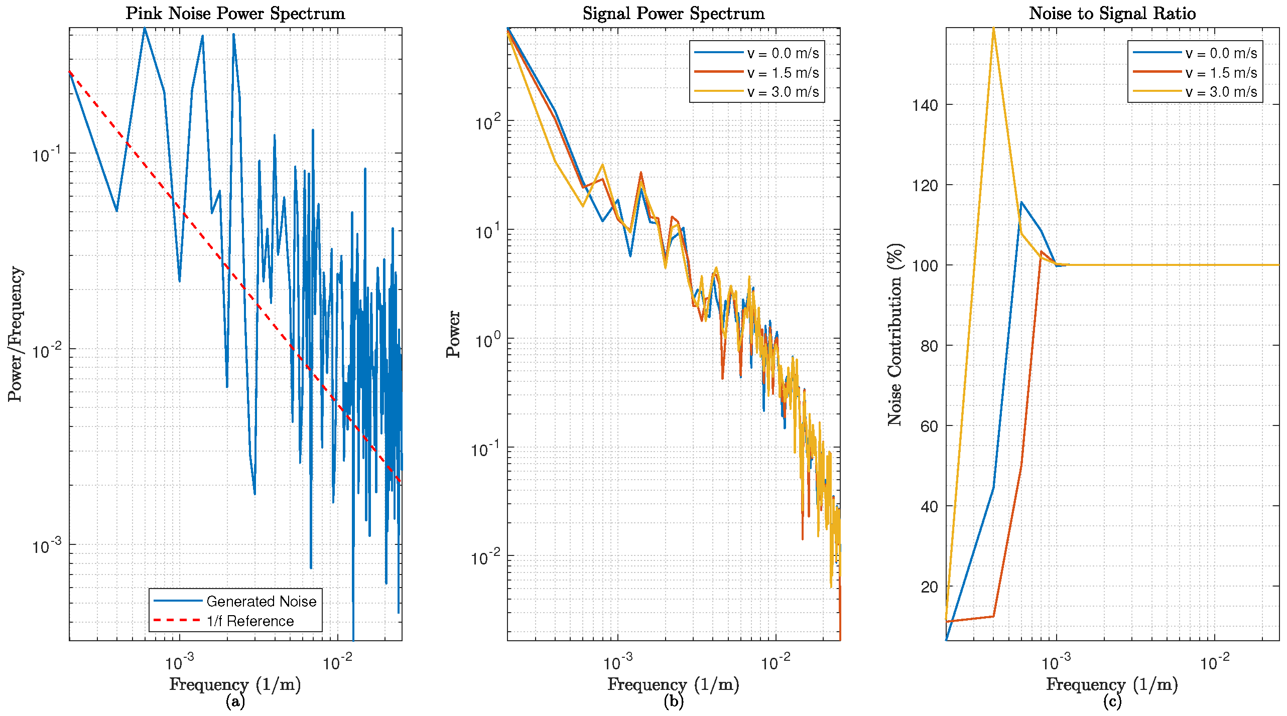
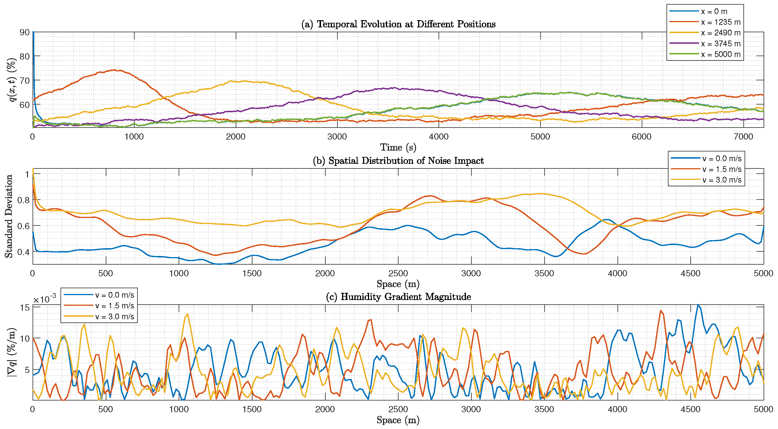
The standard deviation due to pink noise varies spatially: for $v=0\mathrm{m}/\mathrm{s}$, it is 0.5534 at $x=0$, 0.5755 at $x=2500\mathrm{m}$, and 0.5918 at $x=5000\mathrm{m}$. For $v=1.5\mathrm{m}/\mathrm{s}$, the values are 0.9137, 0.7061, and 0.7417, respectively. For $v=3\mathrm{m}/\mathrm{s}$, the values are 1.0399, 0.7220, and 0.7004. This indicates a complex spatial relationship between noise impact and velocity, with higher velocities showing greater variability near the source but more complex patterns inland. The spectral analysis shows power spectral density slopes of approximately $-1.50$, $-1.55$, and $-1.49$ for $v=0,1.5,3\mathrm{m}/\mathrm{s}$, respectively, closely matching the expected behavior of pink noise (slope $\approx -1$) interacting with the fractional dynamics of the system.

4.2. Visualization and Analysis

The following figures illustrate the moisture dynamics and noise effects, ordered to progress from an overview to detailed insights:

Figure 1 provides a detailed analysis for $v=3\mathrm{m}/\mathrm{s}$. Subfigure (a) depicts $q(x,t)$ as a 3D surface, emphasizing temporal and spatial trends of high humidity near the coast that decreases further inland, modulated by noise-induced variability. Subfigure (b) plots spatial profiles at $t=0,1800,3600,5400,7200\mathrm{s}$, illustrating advection-driven shifts and noise fluctuations, with humidity exceeding 80% up to 2242 m by the end.

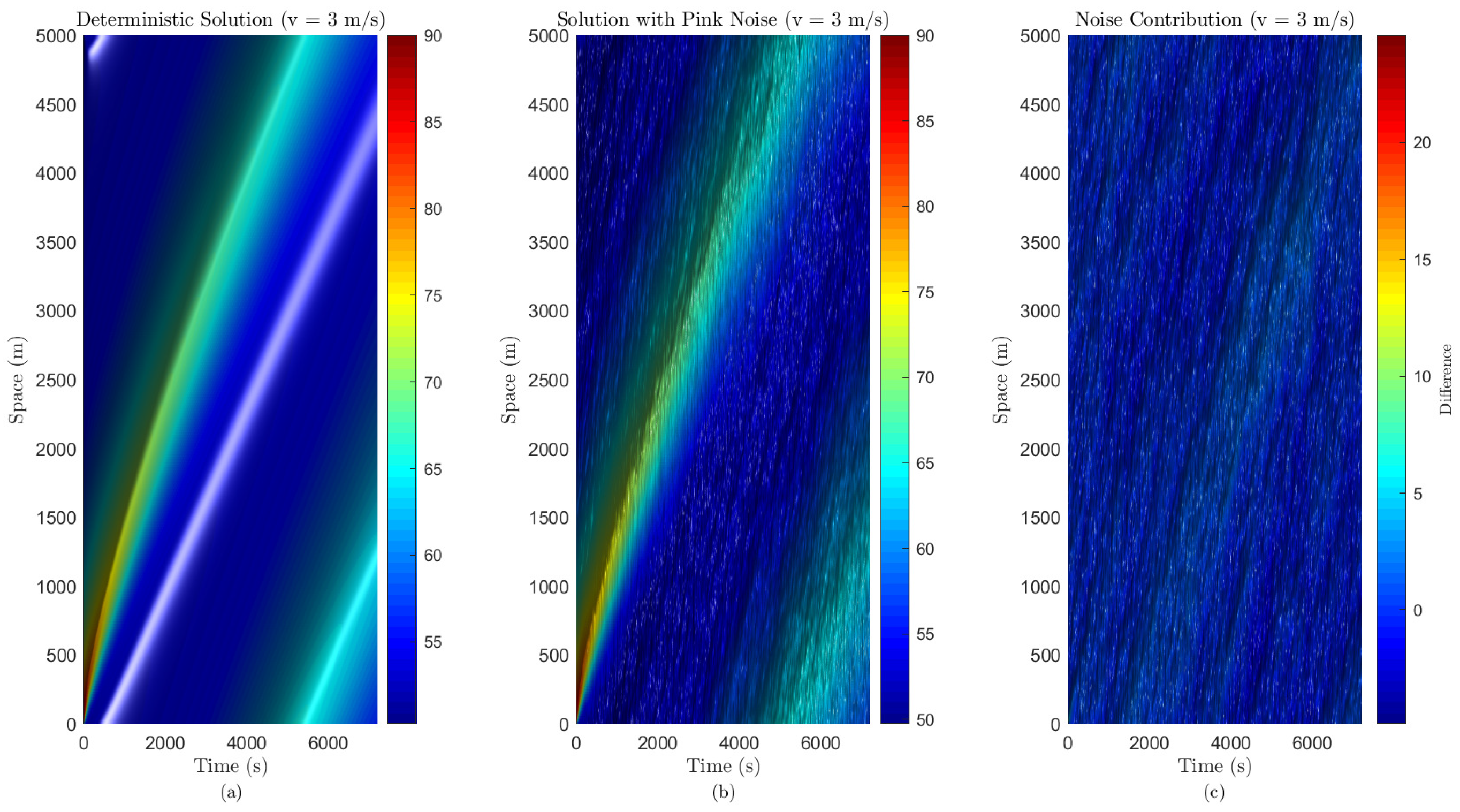
Figure 2 displays heatmaps of $q(x,t)$ for $v=0,1.5,3\mathrm{m}/\mathrm{s}$, showing moisture evolution over space and time. For $v=0$, diffusion dominates, spreading moisture gradually. Increasing v accelerates inland transport, with $v=3\mathrm{m}/\mathrm{s}$ showing significant penetration. The color gradients (parula colormap) highlight humidity levels, with the colorbar indicating percentages. Figure 3 presents the power spectrum analysis. Subfigure (a) confirms the pink noise’s $1/f$ characteristic (slope $\approx -1$) against a reference line, validating its generation. Subfigure (b) shows the signal power distribution across frequencies, with steeper slopes for higher v, reflecting advection’s smoothing effect. Subfigure (c) plots the noise-to-signal ratio (%), peaking at low frequencies and decreasing, illustrating noise’s localized impact.

Figure 4 quantifies the noise effects. Subfigure (a) tracks temporal evolution at $x=0,1250,2500,3750,5000\mathrm{m}$ for $v=3\mathrm{m}/\mathrm{s}$, revealing noise-driven oscillations around the deterministic trend. Subfigure (b) displays the spatial standard deviation, increasing inland due to cumulative noise. Subfigure (c) plots the gradient magnitude $|\nabla q|$ at $t=7200\mathrm{s}$, showing sharper gradients near the coast, softened by advection and noise inland.

Figure 5 compares white and pink noise. Subfigure (a) shows time series samples, with pink noise exhibiting larger low-frequency fluctuations. Subfigure (b) confirms white noise’s flat PSD and pink noise’s $1/f$ decay in log–log plots, justifying its meteorological relevance.

Figure 6 isolates the pink noise effects for $v=3\mathrm{m}/\mathrm{s}$. Subfigure (a) shows the deterministic solution with smooth advection–diffusion. Subfigure (b) includes pink noise, adding realistic variability. Subfigure (c) presents the difference, highlighting noise’s spatial–temporal impact, which is stronger inland.

These visualizations collectively demonstrate the FTSADE (1)’s ability to capture coastal moisture dynamics, with advection enhancing penetration, fractional diffusion accelerating spread, and pink noise introducing realistic variability. Adjusting $\alpha$, $\beta$, or v allows tailoring to diverse atmospheric conditions, supporting applications in weather forecasting.

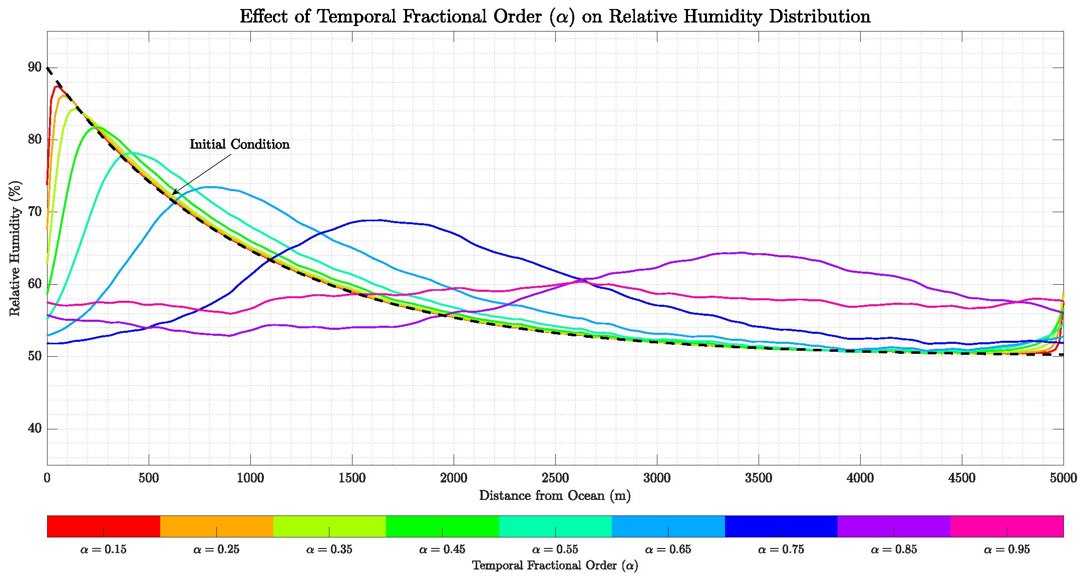
Figure 7 illustrates the influence of the temporal fractional order $\alpha$ on the relative humidity distribution over a 5000-meter domain from the ocean. The parameter $\alpha$ varies from 0.15 to 0.95, with fixed $\beta =1.6$ and wind velocity $v=1.5\mathrm{m}/\mathrm{s}$. The initial condition (black dashed line) shows humidity decreasing from 90% at $x=0$ to approximately 50% inland. Each curve, colored according to the colorbar, represents a different $\alpha$. Higher $\alpha$ values result in smoother profiles, approaching classical diffusion.

4.3. Effect of Spatial Diffusion Exponent

Figure 8 shows the effect of the spatial diffusion exponent $\beta$, ranging from 1.3 to 1.9, with fixed $\alpha =0.85$ and $v=1.5\mathrm{m}/\mathrm{s}$. The initial condition is identical to that in the previous figure. Each curve corresponds to a $\beta$ value, as indicated by the colorbar. Lower $\beta$ values enhance super-diffusion, producing sharper gradients near the ocean, while higher $\beta$ values yield more gradual humidity decay.

4.4. Numerical Convergence Analysis

To evaluate the accuracy and convergence properties of our numerical scheme for the fractional diffusion–advection equation, we conducted a systematic convergence study. The scheme utilizes spectral differentiation in space, implemented via FFT, and a direct integration method for the fractional time derivative. The convergence analysis adhered to the following procedure Algorithm 2:

Algorithm 2 Convergence Analysis Methodology

Step 1: Reference Solution  1: Establish a reference solution of elevated resolution to serve as a benchmark.  2: Compute the solution with spatial discretization $N_x=2^{10}$ (1024) grid points and temporal discretization $N_t=2^{11}$ (2048) time steps, ensuring sufficient fidelity for comparative purposes.      Step 2: Spatial Convergence Analysis  3: Fix the temporal resolution at $N_t=2048$ time steps.  4: for $N_x=2^7,2^8,2^9$ (128, 256, 512) grid points do  5:       Compute the numerical solution with the current spatial resolution.  6:       Quantify the relative $L^2$ error by comparing the solution to an interpolated version of the reference solution.  7: end for      Step 3: Temporal Convergence Analysis  8: Fix the spatial resolution at $N_x=1024$ grid points.  9: for $N_t=2^8,2^9,2^{10}$ (256, 512, 1024) time steps do 10:      Compute the numerical solution with the current temporal resolution. 11:      Calculate the relative $L^2$ error with respect to the reference solution. 12: end for      Step 4: Determination of Convergence Rates 13: Perform logarithmic regression analysis in log-log space to derive empirical convergence rates. 14: Use the functional relationship: $$log\left(E\right)=p·log\left(h\right)+C,$$ (12) where E denotes the relative error, h represents the discretization step size (spatial or temporal), p signifies the order of convergence, and C is a constant offset.

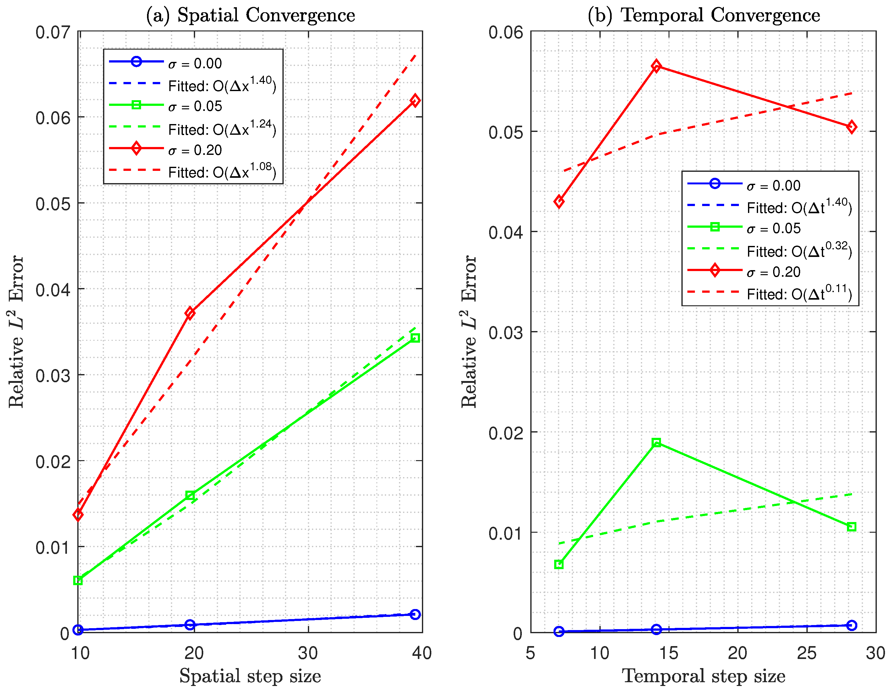
The results of this convergence analysis are presented in Figure 9 for the fractional ADE with stochastic forcing at noise amplitudes of $\sigma =0.00$, $\sigma =0.05$, and $\sigma =0.20$. The analysis reveals distinct convergence behaviors for spatial and temporal discretizations, modulated by the presence and strength of stochastic forcing.

In the deterministic case ($\sigma =0.00$), both the spatial and temporal convergence rates exceed typical expectations, underscoring the scheme’s effectiveness for smooth, noise-free problems. However, as the noise amplitude increases, the convergence rates degrade significantly below the theoretical predictions, particularly at $\sigma =0.05$. This degradation indicates numerical challenges in accurately capturing stochastic effects. Notably, spatial refinement proves more effective than temporal refinement for reducing errors, especially under high-noise conditions ($\sigma =0.20$). These findings offer practical guidance for computational resource allocation in simulations of atmospheric moisture transport with stochastic forcing.

Unlike classical diffusion models ($\alpha =1$, $\beta =2$), which exhibit exponential spatial convergence and $\mathcal{O}(\Delta t^2)$ temporal convergence, our fractional model’s convergence rates reflect the non-local nature of fractional operators and the influence of stochastic effects. The observed degradation in convergence with increasing noise amplitude contrasts sharply with deterministic classical models, highlighting the distinct numerical challenges posed by fractional stochastic systems.

Table 1. Numerical performance of the FTSADE (1) solution for different noise amplitudes ($\sigma$) and grid sizes.

$\mathit{\sigma }$	${\mathit{N}}_{\mathit{x}}$	${\mathit{N}}_{\mathit{t}}$	Relative ${\mathit{L}}_2$ Error	CPU Time (s)	Convergence Order
					Spatial	Temporal
ine 0.00	512	256	2.9668 × 10−4	79.65	1.4043	–
	256	1024	1.0032 × 10−4	31.93	–	1.4036
0.05	512	256	6.0714 × 10−3	83.58	1.2432	–
	256	1024	6.7851 × 10−3	34.35	–	0.3169
0.20	512	256	1.3707 × 10−2	77.75	1.0828	–
	256	1024	4.2983 × 10−2	32.82	–	0.1148

summarizes the numerical performance of the FTSADE (1) solution, computed using FFT and the direct integration method. It reports the relative $L^2$ errors, CPU times, and convergence orders for noise amplitudes of $\sigma =0.00$, $\sigma =0.05$, and $\sigma =0.20$, as derived from the comprehensive convergence study presented above.

5. Results and Discussion

Comprehensive simulations over a coastal domain revealed profound insights into moisture transport dynamics: advection velocity emerges as the dominant factor governing inland humidity penetration, with higher wind speeds significantly extending the reach of elevated humidity levels beyond fog formation thresholds. The fractional parameters $\alpha$ and $\beta$ provide powerful mechanisms for fine-tuning model behavior, with decreasing $\alpha$ amplifying memory effects and lower $\beta$ values intensifying super-diffusive characteristics, offering unprecedented flexibility for calibration to site-specific atmospheric conditions.

The incorporation of pink noise with its characteristic $1/f$ spectrum introduces realistic low-frequency variability, essential for accurate environmental modeling, confirmed through spectral analysis that revealed slopes closely aligning with the theoretical expectations across all advection scenarios. A rigorous convergence analysis demonstrated the numerical scheme’s exceptional accuracy under deterministic conditions, achieving high spatial and temporal convergence rates, though these rates declined under elevated noise conditions. This finding yields an important computational guideline: spatial grid refinement offers substantially greater error reduction than temporal refinement in stochastically forced simulations.

6. Conclusions

This study developed and validated a one-dimensional FTSADE that fundamentally advances the modeling of moisture transport in near-surface atmospheric layers over oceanic boundaries. By integrating fractional calculus with advective dynamics and pink noise stochasticity, the proposed framework successfully captures three critical phenomena that conventional integer-order models fail to represent adequately: long-range temporal dependencies, non-local turbulent mixing, and correlated environmental fluctuations. The mathematical architecture—combining Caputo fractional derivatives, fractional Laplacian operators, and $1/f$ stochastic forcing—provides a theoretically rigorous yet computationally tractable approach to simulating anomalous diffusion processes in atmospheric systems.

The innovative numerical solution methodology, leveraging combined Fourier–Laplace transformations, demonstrates exceptional efficiency by reducing complex fractional operators to algebraic expressions and enabling closed-form solutions via Mittag–Leffler functions. Enhanced by an optimized convolution approximation for stochastic components, this approach strikes an optimal balance between computational feasibility and physical accuracy.

The FTSADE framework represents a significant advancement in atmospheric moisture transport modeling, bridging sophisticated mathematical theory with practical meteorological applications. Its demonstrated capacity to simulate critical phenomena such as coastal fog formation and localized precipitation establishes its value for environmental engineering, hydrological forecasting, and meteorological prediction. Future research directions include multi-dimensional extensions, the implementation of variable wind fields, and the exploration of alternative noise profiles to further enhance real-world applicability. This study lays a robust foundation for the broader adoption of fractional stochastic models in geophysical sciences, revealing their exceptional potential to elucidate and predict the complex transport processes that govern our natural environment.