Abstract
Rheological complex models of various elastoviscous and viscoelastic fractional-type substances with polarized piezoelectric properties are of interest due to the widespread use of viscoelastic–plastic bodies under loading. The word “overview” used in the title means and corresponds to the content of the manuscript and aims to emphasize that it presents an overview of a new class of complex rheological models of the fractional type of ideal elastoviscous, as well as viscoelastic, materials with piezoelectric properties. Two new elementary rheological elements were introduced: a rheological basic Newton’s element of ideal fluid fractional type and a basic Faraday element of ideal elastic material with the property of polarization under mechanical loading and piezoelectric properties. By incorporating these newly introduced rheological elements into classical complex rheological models, a new class of complex rheological models of materials with piezoelectric properties described by differential fractional-order constitutive relations was obtained. A set of seven new complex rheological models of materials are presented with appropriate structural formulas. Differential constitutive relations of the fractional order, which contain differential operators of the fractional order, are composed. The seven new complex models describe the properties of ideal new materials, which can be elastoviscous solids or viscoelastic fluids. The purpose of the work is to make a theoretical contribution by introducing, designing, and presenting a new class of rheological complex models with appropriate differential constitutive relations of the fractional order. These theoretical results can be the basis for further scientific and applied research. It is especially important to point out the possibility that these models containing a Faraday element can be used to collect electrical energy for various purposes.
Keywords:
new class of rheological complex models of ideal materials of the fractional type with polarization property; ideal fluid; Faraday element with property of polarization; differential constitutive relation fractional order; internal degrees of freedom; energy dissipation; Kelvin–Voigt–Faraday model; Maxwell–Faraday model; Lethersich–Faraday model; Jeffrey–Faraday viscoelastic fluid model; Jeffrey–Faraday-F model; Burgers–Faraday model 1. Introduction
The inspiration for the design and construction of a new class of rheological complex model materials came from a lesson on classic rheological complex models contained in a chapter of the author’s university publication on elastodynamics [1], which was used to convey knowledge about rheological complex models to mechanical engineering students.
This new article provides a complete overview of a new class of fractional-type rheological complex material models with piezoelectric properties, providing complete mathematical descriptions and derivations of the fractional order, with all of the details explained for each of the new complex material models.
The author and their coauthors previously researched the dynamics of oscillating certain rheological discrete dynamic systems with one and more degrees of freedom of oscillation, of the fractional type, applying a mathematical description with differential equations of the fractional order. For details, see References [2,3,4,5]. It has been shown through new research results on the topic of elements of mathematical phenomenology and analogies of electrical and mechanical oscillators of the fractional type with a finite number of degrees of freedom of oscillation that there are linear and nonlinear modes; for details, see Reference [4].
In our previously published Reference [5], in the introductory part, we pointed to the list of references and their contents, which were inspirational for researchers and helped to achieve the new results shown in that area, as well as those that we will show in this article, so we will not list them here, nor are they included in the present list of references.
In our work in Reference [5], titled “Rheological Burgers–Faraday models and rheological dynamical systems with fractional derivatives and their application in biomechanics”, two rheological Burgers–Faraday models and the dynamics of two rheological discrete dynamical systems were created by using, without more detail, two new rheological models: a Kelvin–Voigt–Faraday fractional-type model and a Maxwell–Faraday fractional-type model. The Burgers–Faraday models described, also without more detail, in the paper are new models of the dynamical behavior of materials with coupled fields: mechanical normal stress and axial dilatation and the electric field of polarization through Faraday’s element. An analysis of the constitutive relation of differential fractional orders for Burgers–Faraday models is given, in brief.
This new article includes those models, but also with new details of mathematical descriptions and the derivation of differential constitutive relations of the fractional order and determination of their solutions, which were not presented in the previous published article [5]. This completes the presentation and overview of all of the new rheological complex models of the fractional type with piezoelectric properties, which belong to a new class of complex material models with the property of polarization of the piezoelectric elements contained in those models.
We should also mention References [6,7], of which the group of authors’ common contribution is given in the mathematical field of fractional calculus with applications in mechanics, particularly vibrations and diffusion processes, as well as wave movements in continuums.
Using the previous definition of the differential operator of the fractional order, we introduce an ideal new fluid element, Newton’s ideal viscous element, based on the differential constitutive relationship between the normal stress and the velocity of axial dilatation (fractional type).
The piezoelectric materials are used for modeling new types of rheological models of materials. It is known that piezoelectric materials have coupled tensors of mechanical and electrical states; for details, see Reference [8]. The relationships between the elements of the tensor of the mechanical stress state and the tensor of the mechanical deformation state in coupling with the tensor of the electrical state of polarization were studied for samples with different direction of polarizations; see Reference [8].
Today, the application of piezoelectric materials is widespread and they are productively used in various fields of technology and medicine, as sensors, actuators, and exciters; see References [3,5].
In addition to the keyword of the fractional type, we will often use the word Faraday, so we provide basic information about the famous scientist Michael Faraday (22 September 1791–25 August 1867).
Faraday was an English bookbinder who became interested in electricity (for details, see References [9,10]). He earned the title of assistant in Davy’s laboratory, and at the age of 19, Faraday studied with the renowned chemist Sir Humphry Davy (Sir Humphry Davy, 17 December 1778–Geneva, 29 May 1829), president of the Royal Society, and John Tatum, founder of the Civil Philosophical Society. Then, he began to conduct his own experiments. He was the first to discover that electricity produces an electrical “tension” (electric voltage), which produces an “electrotonic state”, or the polarization of matter molecules.
For the formation of complex rheological models of fractional-type materials with piezoelectric properties, we introduced a new rheological element, which we called Faraday’s rheological ideal elastic element with polarization ability and piezoelectric properties. This will be discussed in the next chapter.
Therefore, to begin with, we provide a basic short presentation of some publications on rheological complex models of the fractional type, which we will modify by parallel or series coupling with the newly introduced rheological Faraday element—an ideal elastic element with polarization capability [5].
From the published literature, we learned that rheological models are used to describe the models and compositions of building materials, yarns in the textile industry, and biomaterials. Reference [11] shows the use of ultrasonic piezoceramic materials in a practical model of an ultrasonic sprayer design. An auxiliary size distribution model for the ultrasonically produced water droplets was experimentally tested. Reference [11] inspired the author of this paper in the introduction of the new Faraday element. This sprayer design using an ultrasonic oscillator allows the formation of a new design of a fractional-type ultrasonic sprayer with piezoelectric properties in which the concentrator of variable cross-section is a fractional-type rheological element.
The contents of References [12,13,14,15] present research on rheological models in civil engineering, from studying rheological models of soft rock matrix creep [16,17] to studying composite and prestressed structures using rheological modals and presenting the corresponding classification of the rheological models used [13].
In his doctoral dissertation [18], entitled “Dynamic Behavior of the Mechanism System—the Working Object of the Weaving Process”, the author studied the dynamics and use of several rheological models of textile fibers, with which he demonstrated their use in the textile industry, while in [19], he studied the rheological modeling of yarn elongation.
Reference [20], entitled “Review: Rheological properties of living materials. From cells to tissues”, as well as Reference [21], entitled “New rheological problems involving general fractional derivatives with nonsingular power-law kernels”, present the applications of rheological models in biomaterials.
The content of [22], entitled “A fractional model for time-variant Non-Newtonian Flow”, presents new results and insights into the behavior of certain rheological models: as the author calls them, models of Non-Newtonian Flow. Reference [23] presents the results of the research of the group of authors entitled “A unified rheological model for cells and cellularised materials” and provides insights into the basic models of rheological biomaterials. The group of authors in Reference [24], entitled “Fractional rheology-informed neural networks for data-driven identification of viscoelastic constitutive models”, presents new results using fractional rheological models.
The author in Reference [25] presents the results of research and modeling of thermorheological models and thermomechanical systems using fractional-order differentials.
The following conclusions can be drawn from the published literature: First, the majority of published papers on rheological models of ideal materials refer to classical complex rheological models, which are presented in integral form, in one chapter of a university textbook [1] on the Theory of Elasticity. Second, most of the papers on rheological models are regarding applications in construction, on concrete and rock materials, and then in the textile dyeing industry with application to cotton and yarn (see References [18,19]).
The complete and integral theory of the Analytical Dynamics (Mechanics) of Discrete Hereditary Systems is presented in Reference [26], as well as some experiments to determine the kernel of theology for different rheological materials’ hereditary properties.
The generalized function of fractional-type dissipation of system energy is presented in Reference [27].
The previously cited Reference [8] contains significant knowledge about the coupled fields of mechanical and piezoelectric states.
The citation and presentation of the contents of the references from the above-mentioned list of references, which were available to the author, provide sufficient evidence of the uniqueness and originality of the author’s new scientific results presented in this manuscript. At the same time, the author is free to emphasize that the scientific results presented in this manuscript are the result of spontaneous scientific inspiration and knowledge acquired during the author’s more than half a century of dedication to science. In this sense, the list of references is only a description of the contents contained in these published references.
These rheological complex models of materials of the fractional type with piezoelectric polarization properties are suitable for studying the behavior of complex systems such as rheological oscillators or creepers of the fractional type. In addition, the obtained rheological complex models of materials also open possibilities to create numerous new materials whose performance characteristics are primarily based on combinations of their elastic, viscous, viscoelastic, elastoviscous, fractional-type, or even piezoelectric properties.
The theoretical research and scientific results on a new class of rheological complex models of fractional-type materials with piezoelectric properties, which the author presents in this paper, represent, the author emphasizes, the basis and inspiration for applications in real-world technologies, such as materials science, engineering, or biomedical applications. Of course, these results will become the basis for experimentalists to investigate this new class of material models and compile studies of the parameters of each of the theoretical models with the aim of designing technologies for practical applications in engineering and in technologies of biomedical materials with piezoelectric properties.
2. The Purpose of the Work
The purpose of the work is to make a theoretical contribution by introducing, designing, and presenting a new class of rheological materials with piezoelectric properties and corresponding differential constitutive relations.
These theoretical results can be the basis for further scientific and applied research and help provide new contributions to science and applications in various fields of technical and natural sciences, as well as in medicine. It is especially important to point out the possibility that these models containing Faraday’s elastic and piezoelectric element, through their polarization and the effect of mechanical loading and deformation, are able to collect electrical energy that can be used for various purposes, for example, for lighting bridges, for spraying fluids in conjunction with ultrasonic sprayers to refresh lawns in parks, or for covering disco club spaces and the like.
The dynamics of the newly introduced class of rheological complex models of fractional-type materials and piezoelectric properties, in this work, is theoretically studied in isothermal conditions, at constant temperature and with fractional-type properties of mechanical energy dissipation.
3. Methodology
In this manuscript, we have outlined the basics of the methodology used to carry out our set of research tasks and to describe and compile differential constitutive relations of the fractional order. Firstly, it is necessary to explain how these differential constitutive equations of the fractional order compiled when the basic elements of the structure of basic and complex rheological models of materials are connected in parallel or in series. Then, by decomposing the complex structure of the model to enable parallel connection of rheological elements, we assumed that the resulting normal stress could be obtained as the sum of the component normal stresses in the rheological elements connected in parallel. From there, we determined the differential constitutive relation of the fractional order with piezoelectric properties.
We also show, by introducing the decomposition of the velocities of axial dilatations of the fractional type, that the resulting axial velocity of the fractional-type dilatations is obtained as the sum of the component axial velocities of the fractional-type axial dilatations of the rheological elements connected in a regular manner in a complex material model. From there, the differential constitutive relation of the fractional order is obtained for the regular rheological models. We see that two approaches and two methods for describing the dynamics of the rheological complex material model and compiling the differential equations of the constitutive relations of the fractional order are used. These two methods are used to analyze the physical properties of rheological complex materials of the fractional type with piezoelectric properties. For the next phase of studying this new rheological complex model’s materials, a mathematical description was formulated consisting of one or more differential equations that need to be solved. To solve these differential relations, we used the methods of Laplace transform and inverse Laplace transform. To obtain approximate analytical expressions for the solution of the constitutive relations, we used the expansion in power series of the parameters of the Laplace transforms. We also used the expression for the inverse Laplace transform of the power.
Next, we will provide some basic information about differentiation of the fractional order, as it will be one of the most frequently used terms in this manuscript.
Differentiation of the fractional order, although it first appeared in the scientific communications of Leibniz and the Marquis L’Hospital, has only recently gained wider application in various fields of science and technology, as in References [3,4,28,29]. A brief story about the operators of generalized fractional calculus is presented in [30], while [31] decribe an application of Fractional calculus as an introduction for physicists. Generalized Fractional calculus and applications are in [32]. The analysis of fractional differential equations and fractional equations and models are presented in [33,34]. Numerical methods for Fractional calculus are described in [35,36].
Today, there are different definitions of differentiating a fractional order. For basic knowledge about differentiating a fractional order, it is very useful to read the following articled [37,38,39,40], which present the mathematical foundations and some of the applications in continuum mechanics. Publication [41,42] present generalized Mittag-Leffler functions and their properties, which are often used in some transformations of fractional order derivative expressions. For approximate calculations of some expressions with fractional order differentials, it is necessary to use numerical methods, see scientific publications [43,44,45,46], which contain some of the new numerical methods. Reference [47] contains results on Summation identities for the Kummer confluent hypergeometric function, which are useful in the application of numerical methods.
Publications [48,49] present the coupled tensors of the piezoelectric material mechanical states and electrical voltage, and their applications in ultrasonic transducers with applications in sprayers and other devices.
For background information on Michael Faraday, see References [50,51].
Articles [16] presents a classification of classical rheological models of materials in civil engineering with corresponding definitions, while
References [17,52,53] present the properties of complex structures, various classical rheological models of their creep, and their applications to civil engineering materials.
It should be noted that rheological models can also be used in the textile industry to describe yarn dynamics. The results of the application of classical linear rheological models to the study of yarn dynamics in the textile industry are given in References [54,55], for example, under the title: “Rheological modeling of yarn elongation” or “Dynamic behavior of the mechanism–Working object system of the weaving process”.
In Reference [56], the application of new rheological models of materials to biomaterials is presented, under the title “New rheological problems involving general fractional derivatives with nonsingular power-law kernels”.
In this paper, we use Caputo’s definition of the derivative of the fractional order over the differential operator of the fractional order, which we denote by , in the following form:
For example, , in which is determined as an exponent, in interval . If in the previous Equation (1), the exponent , then the application of the differential operator of the fractional order gives the first-time derivative of the time function to which it is applied. In terms of the differential operator of the fractional order, when its exponent of the fractional order is formed of rational numbers and is in the interval , including its limit values, it can be useful as a mathematical description in various applications. In the previous definition of the differential operator of the fractional order, the special function represents a special Gamma function, which is defined in the form of an integral (see Reference [57]):
which is a function of the exponent of the differential operator of the fractional order, or in the general case, is a function of the variable , in the following form:
Let us also mention the important references in which numerical methods for calculating derivatives of the fractional order are shown and explained, such as the following References [58,59,60,61,62].
In this work, we used analytical methods and analytical approaches, but researchers have access to new numerical methods and commercial software that can be used to study the dynamics of rheological complex model materials.
4. New Newton Element and Faraday Element with Polarization Properties
In this part of the paper, we introduce and use two new elementary rheological elements, one of which is the fractional type and the other ideal elastic with piezoelectric properties. These two new elementary rheological elements are the rheological basic Newton element of an ideal fluid, which is fractional type, and the basic Faraday element of an ideal elastic material with coupled mechanical and electrical fields, exhibiting polarization under mechanical loading and piezoelectric properties.
By introducing these newly introduced rheological elements into classical complex rheological models, a new class of complex rheological models of the fractional type with piezoelectric properties was obtained.
In this paper, also, we introduce the following new class of complex rheological fractional-type models with piezoelectric properties: 1*—a complex basic rheological Kelvin–Voigt–Faraday fractional-type model of elastoviscous solid material with piezoelectric properties; 2*—a complex basic rheological Maxwell–Faraday fractional-type model of viscoelastic fluid with piezoelectric properties; 3*—a complex rheological Lethersich–Faraday fractional-type model of viscoelastic fluid with piezoelectric properties; 4*—a complex rheological Jeffrey–Faraday fractional-type model of viscoelastic fluid with piezoelectric properties; 5*—a rheological complex Jeffrey–Faraday-F fractional-type model of an elastoviscous solid body with piezoelectric properties; 6*—a rheological complex Burgers–Faraday fractional-type model of viscoelastic fluid with piezoelectric properties; and 7*—a rheological complex Burgers–Faraday-F fractional-type model of an elastoviscous solid body with piezoelectric properties.
This new element of a Newtonian ideal viscous fluid is of a fractional type. The axial flow of the fractional-type fluid, which is stressed axially, has normal stress at the points of transverse transitions of the fluid flow and the fractional-type axial dilatation velocity of line elements of the fluid is in the axial direction. The constitutive relation is and is in differential-fractional-order form. This differential-fractional-order constitutive relation shows the connection between the normal stress in the axial flow of the fluid in the cross-section of the fluid flow and the velocity of the fractional-type axial dilatation of the linear elements of the fluid in the axial direction of the linear element flow of the fluid. The material constant is the viscosity coefficient of the fractional-type fluid and is determined experimentally for each fluid.
The basic dimensions of the measurements are as follows: for normal stress, , at the cross-sections, fractional-type fluid flow is measured in forces per unit area; for the fractional-type axial velocity of dilatation of the line elements in the axial direction of the fractional-type fluid flow, the length increment is given by the total length, and the unit of time depends on the exponent of the order of fractional differentiation, or can be a dimensionless quantity; and for the viscosity coefficient , it can be given in forces per square of length or surface area, and the unit of time, to a degree, corresponds to the order of fractional differentiation (see Figure 1c).
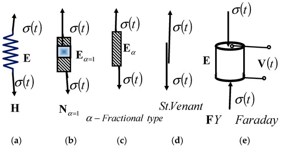
Figure 1.
Basic rheological elementary elements: (a) Hooke’s ideal elastic solid body, (b) Newton’s element of an ideal linear viscous fluid, and (d) Saint Venant’s ideal plastic material, as well as (c) the new rheological basic Newtonian model of a fractional-type ideal viscous fluid and (e) the basic Faraday element with coupled mechanical and electrical fields of an ideal elastic solid material and with piezoelectric properties.
Let us denote by the rheological Faraday element with coupled mechanical and electrical fields of an ideal elastic solid body with polarization under mechanical loading and deformation and exhibiting piezoelectric properties. When a test tube made of this piezoelectric material is subjected to axial normal stress, due to ideal elasticity, axial dilatation occurs, as well as deformation of the crystal lattice of the material, and due to ideal piezoelectricity, axial polarization of the transverse contour surfaces occurs, and electric voltage and dielectric displacement occur.
The normal stress at the points of the cross-sections can be denoted by , the axial dilatation of the axial line elements by , the electric polarization voltage by , and the dielectric displacements by . As such, the constitutive relations of the rheological Faraday ideal elastic and ideal piezoelectric elements can be expressed as follows: the relation between the electric polarization voltage and mechanical normal stress is , while the relation between the axial dilatation and the electric polarization voltage is .
These constitutive relations are linear and provide a connection between the mechanic state of normal stress and axial dilatation and the electrical state of electric voltage of the electric field of the piezoelectric material. The symbols , , and are the constants of the piezoelectric material, mechanical and electrical, and are determined experimentally. The units , , and are the units of the ideal elastic and ideal piezoelectric material constants.
In this paper, as we indicated in the Introduction, we will use the derivatives of the fractional-order functions and the fractional-order differential operator in order to describe the constitutive relation of the newly introduced viscous element of the fractional type, which we called the rheological Newton viscous element of the fractional type, with the constitutive relation of the normal stress connection and axial dilatation , i.e., the rate of axial dilatation of the fractional type in the form , where the differential operator of the fractional order is , and the fractional-order differentiation exponent has values greater than zero and less than or equal to one (), in accordance with Equation (1).
New complex rheological models of ideal materials with piezoelectric properties are obtained through parallel or serial linking of new, more complex models of the fractional type with the basic Faraday model with ideal piezoelectric properties.
5. New Class of Complex Rheological Models
We will form two basic complex rheological models of the fractional type with piezoelectric properties by connecting two basic complex rheological models, the Kelvin–Voight or Maxwell model (both fractional type), in parallel, respectively, with Faraday’s ideal elastic and piezoelectric material model—or another simple element with piezoelectric properties. The structures of these basic complex models with piezoelectric properties are shown in Figure 2 and Figure 3.
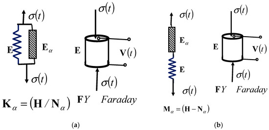
Figure 2.
Structure of two basic complex fractional-type rheological models with piezoelectric properties: (a) basic complex Kelvin–Voigt model of a solid material with the Faraday element and (b) basic complex Maxwell model of a viscoelastic fluid with the Faraday element; these can be connected in parallel or series with Faraday’s ideal piezoelectric material element to obtain new rheological complex models.
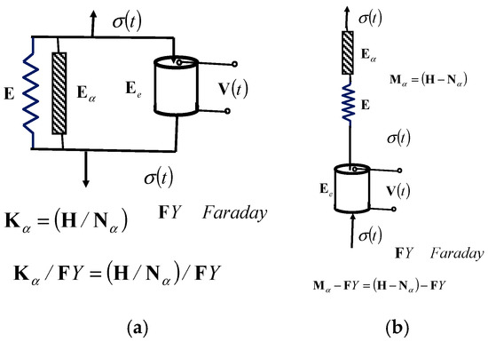
Figure 3.
Two new complex fractional-type rheological models with piezo-electric properties: (a) parallel connection structure of basic complex Kelvin–Voigt solid material model, in parallel connection with Faraday’s element, forming the new complex Kelvin–Voigt–Faraday model of a solid material; (b) series connection structure of the basic complex Maxwell model of viscoelastic fluid material, in series connection with Faraday’s element, forming the new complex Maxwell–Faraday model of a viscoelastic fluid material.
Here, we will study the properties of two new fractional-type complex rheological models with piezoelectric properties: a basic fractional-type complex rheological Kelvin–Voigt–Faraday solid model, an ideal piezoelectric model material, and a basic fractional-type complex rheological Maxwell–Faraday model of a viscoelastic fluid, which is also an ideal piezoelectric model material.
The first model has the parallel connection structure of the basic fractional-type complex rheological Kelvin–Voight solid model in parallel connection with Faraday’s ideal piezoelectric model material, as shown in Figure 2a and Figure 3a.
The second one has the series connection structure of the basic complex rheological Maxwell model of a fractional-type viscoelastic fluid material in series connection with Faraday’s ideal elastic and piezoelectric material element, as shown in Figure 2b and Figure 3b.
The constitutive relations of the normal stress and axial dilatation , i.e., the velocity of axial dilatation of the fractional type, are given in the following form (see Figure 2 for more details on the model compositions):
where is the differential operator of the fractional-order exponent , determined by Equation (1), where the fractional-order differentiation exponent has values greater than zero and less than or equal to one ().
5.1. New Basic Complex Rheological Kelvin–Voigt–Faraday Model of the Fractional Type with Piezoelectric Properties
The structural formula of the rheological complex Kelvin–Voigt–Faraday fractional-type model with piezoelectric propertied is .
The resulting normal stress at the ends of the basic rheological complex Kelvin–Voigt–Faraday model, consisting of the basic rheological complex Kelvin–Voigt fractional-type model in parallel with the Faraday ideal elastic and piezoelectric material element, is equal to the sum of the normal stresses of the elements connected in parallel (see Figure 2a, Figure 3a, and Figure 4a,b).
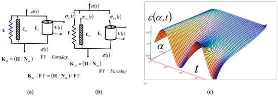
Figure 4.
Rheological basic complex Kelvin–Voigt–Faraday fractional-type model with piezoelectric properties: (a) structure of the model; (b) decomposition of the model; (c) subsequent elasticity of the material’s surface.
In addition, the electric polarization voltage in Faraday’s ideal piezoelectric material element is equal to
Equation (6) is a differential constitutive relation of the fractional order and gives the relationship between the normal stress of the fractional-type rheological basic complex Kelvin–Voight–Faraday model with piezoelectric properties and the axial dilatation , or the axial dilatation rate of the fractional-type material, . It is a constitutive relation of the fractional order, as follows:
The fractional-order differential constitutive relation given in Equation (8) for the rheological basic complex Kelvin–Voigt–Faraday model, a complex rheological material, is in the general form. By applying the Laplace transform to the previous differential constitutive relation given in Equation (8), we obtain the Laplace transform of the axial dilatation of that model as a differential function of the Laplace transform of the normal stress, in the following form:
where is the Laplace operator in the following form:
This Laplace operator can be applied to the following expression:
Equation (9) is the product of two Laplace transforms: one Laplace transform, , is of the normal stress , and the other, , which concluded that these two functions and are also in convolution with the axial dilatation function . As such, the following equation can be derived:
The expression is much smaller than one; that is, . Therefore, we can expand the expression to powers of the order and write it in the following form (see Reference [27]):
Next, the inverse Laplace transform of the previous Equation (13) can be obtained in the following form:
Based on the property of the three functions, which are in convolution and for which it is true that
we can write the convolution integral in the following form:
Both Equations (15) and (16), i.e., the convolution integrals, are integral constitutive equations relating the axial dilatation and normal stress of the rheological basic complex fractional-type Kelvin–Voigt–Faraday model with piezoelectric polarization properties.
The Faraday element in the complex Kelvin–Voigt–Faraday model of the fractional type, due to deformation, axial dilatation , and normal stress , enters a state of polarization, with its axial dilatation calculated using Equation (17), and the electric voltage stored in that element is expressed in the following form:
In the resting case of a rheological basic complex Kelvin–Voigt–Faraday fractional-type model in parallel with Faraday’s ideal elastic and piezoelectric model of the material at a very slow load change, when we can assume that the fractional-type axial dilatation rate is small and tends to zero (), the material behaves as a basic ideal elastic material, and the normal stress of the material is almost proportional to the dilatation :
If the normal stress at the ends of a rheological basic complex Kelvin–Voigt–Faraday model, in the case where it is in parallel with the Faraday ideal piezoelectric material element, suddenly rises from zero to some finite value, , which remains constant in the following time interval, then we are interested in the behavior of this basic model of the complex material.
If we assume that the normal stress rises suddenly to some value and remains constant , then the following can be determined:
In order to find the time dependence of the axial dilatation of the rheological basic complex Kelvin–Voigt–Faraday fractional-type model, in parallel with Faraday’s ideal piezoelectric material element, we first apply the Laplace transform to the previous differential fractional-order constitutive equation and obtain the Laplace transform of axial dilatation in the following form:
The solution for the axial dilatation as a function of time for the basic complex Kelvin–Voigt–Faraday model, in parallel with Faraday’s element, when suddenly subjected to a constant normal stress and held at a constant normal stress , is the inverse Laplace transform of Equation (21):
Next, it is necessary to determine the approximate analytical expression for the time function as the inverse Laplace transform of the previous expression and transfer it into the time domain.
As such, it is necessary to develop the expression in order by powers of , which is a complex number, using the formula (see References [4,5,57,63]). As such,
The inverse Laplace transform now gives an analytically approximate expression for the time-domain axial dilatation for the basic complex rheological Kelvin–Voigt–Faraday fractional-type model with piezoelectric properties, when suddenly subjected to a constant normal stress and kept under constant normal stress in the following form:
The dielectric displacement (shift) , represented as and in the polarized Faraday element included in parallel in the basic complex rheological Kelvin–Voigt–Faraday fractional-type model with piezoelectric properties, can be expressed in the following form:
This model of a complex rheological Kelvin–Voigt–Faraday material of the fractional type with piezoelectric properties, with the parallel connection structure of the basic complex rheological Kelvin–Voight model of a solid elastoviscous fractional-type material in parallel connection with Faraday’s ideal piezoelectric material model, possesses the property of post-elasticity, when axial dilatation lags behind normal stress .
In Figure 4c, the surface of the subsequent elasticity of that basic complex rheological Kelvin–Voigt–Faraday material of the fractional type with piezoelectric properties is presented in a coordinate system with coordinate axes: the elongation of axial dilatation , the exponent of fractional-order differentiation, in an interval greater than zero and less than or equal to one (), and time.
The rheological complex Kelvin–Voigt–Faraday fractional-type model, with piezoelectric properties has no internal degree of freedom.
5.2. New Basic Complex Rheological Maxwell–Faraday Model
We will now further study the properties of a new basic complex rheological model, a fractional-type model with piezoelectric properties that has a series connection structure of the basic complex rheological Maxwell model of a viscoelastic fluid material, a fractional type model, in series connection with a Faraday ideal elastic and piezoelectric model material. As a result, a new rheological basic complex Maxwell–Faraday model, a fractional-type model with piezoelectric properties, is obtained. See Figure 2b and Figure 3b.
Throughout the entire basic complex model with the Hooke ideal elastic element , the Newton viscous element of the fractional type , and the Faraday ideal elastic and piezoelectric material element, the normal stress in all the regularly connected elements is the same, while the resulting fractional-type dilatation velocity is equal to the sum of the dilatation velocities of the elements , , and in the order connection. Figure 5b shows the component dilatations of these regularly connected elements of the complex rheological complex basic Maxwell–Faraday model of the fractional type.
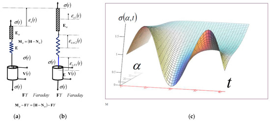
Figure 5.
Rheological basic complex Maxwell–Faraday fractional-type model with piezoelectric properties: (a) structure of the model; (b) decomposition of the model; (c) normal stress relaxation of the model’s surface.
Faraday’s ideal elastic and piezoelectric material model was added to a rheological basic complex Maxwell’s model of the fractional type, whose structural formula is , to create a new rheological basic complex Maxwell–Faraday model.
When using Hooke’s ideal elastic solid element , Newton’s fractional-type viscous element , and Faraday’s ideal elastic and piezoelectric material element, throughout the entire basic complex model , the velocity of axial dilatation of the fractional type through the entire element is equal to the sum of the axial dilatation velocities of the elements, , , and in a regular series connection, so in the sum of the axial dilatation rates, we use the dilatation rates of the fractional-type equation . See Figure 5a,b. In Figure 5b, the decomposition of the axial dilatation of the new rheological basic complex Maxwell–Faraday model is presented and component dilatations are visible.
The normal stress is the same throughout the entirety of the new rheological basic complex Maxwell–Faraday model of the fractional type with piezoelectric properties, so we can determine the differential constitutive relations of each basic rheological element in this series connection; as such, the same normal stresses are a function of the resulting dilatation of the model (see Figure 5b):
The differential constitutive relations between the normal stress and velocity axial dilatation of the fractional type (see Figure 5b for an illustration of the idea of decomposition by dilatations) of each of the regularly connected elements of the complex structure of the Maxwell–Faraday model are determined by Equation (26), as shown previously.
For Hooke’s ideal elastic element, the normal stress is and is linearly related to the dilatation, and the velocity of fractional-type dilatation is a function of the normal stress of the fractional-type equation . For the new ideal viscous Newtonian element of the fractional-type fluid, the normal stress is differentially related by fractional order to the velocity of fractional-order axial dilatation . The velocity of fractional-type axial dilatation is expressed in terms of the normal stress . For the ideal elastic Faraday element with piezoelectric properties, the mechanical normal stress is linearly related to the axial dilatation and the electrical voltage due to the polarization of the Faraday element by mechanical strain, and also the dielectric displacements and are linearly related to the mechanical normal stress or dilatation. For this Faraday element, the velocity of fractional-type axial dilatation is a function of the velocity of fractional-type normal stress in the form .
The electric voltage can be expressed as and the dielectric displacement (shift) as , , and in the polarized Faraday’s element included in serial in the basic complex model.
Figure 5a presents the basic complex Maxwell–Faraday model and Figure 5b presents the decomposition into component axial dilatations of rheological elements of the basic complex Maxwell–Faraday model of the fractional type with piezoelectric properties. This figure shows and explains how the differential constitutive relations of the fractional order are constructed.
The resulting velocity of axial dilatation of the basic complex Maxwell–Faraday model of the serial structure is equal to the sum of the component fractional-type axial dilatation velocities of Newton’s fractional-type viscous element , of Hooke’s ideal elastic element , and of Faraday’s ideal elastic element with the property of piezoelectricity, and can be expressed in the following form:
As such, and therefore , , and , resulting in . Therefore, the sum can be expressed as follows (see Figure 5b):
Next, based on the previous analysis, it follows that this sum of fractional-type axial dilatations in the rheological basic complex Maxwell–Faraday model is of the following form (see Figure 5b):
The last inhomogeneous ordinary differential Equation (29) of the fractional order is a differential constitutive relation of the fractional-order exponent , highlighting the axial dilatation and normal stress relationship of the rheological basic complex Maxwell–Faraday model of the fractional type with piezoelectric properties.
The last inhomogeneous differential constitutive equation, Equation (29), of fractional-order exponent can be solved by applying the Laplace transform , which gives the following:
Then, expanding in order by powers of the complex parameter, we obtain the following:
Using the property of the three functions being convolved, as well as the relationship between their Laplace transforms and the convolution integral, in a similar way as in [5], we can produce the following convolution integral:
Equation (32), which is the convolution integral, represents an approximate analytical expression of the dependence of the normal stress in the basic complex Maxwell–Faraday model, as a function of the total axial dilatation over time, and is also the constitutive integral equation of that model.
If the material in the basic complex Maxwell–Faraday model is suddenly loaded to a certain value of normal stress , it will respond to an elastic deformation, , created instantaneously in Hooke’s ideal elastic element and Faraday’s piezoelectric element. This is because due to a sudden load added immediately at the beginning of the observation of the behavior of the material of the basic complex Maxwell–Faraday model, flow in the regularly connected modified Newton viscous element, in this case, in the viscous fluid, does not come to the fore. If we prevent the development of axial dilatation, assuming that the velocity of axial dilatation tends to zero, , then the normal stress is a function of time, which needs to be determined.
When the normal stress rate of the fractional type of the rheological basic complex Maxwell–Faraday model tends to zero, , then the normal mechanical stress tends to a value proportional to the axial dilatation rate of the fractional type, :
In order to find the dependence of the normal stress on time, when we keep the model of the material of the rheological basic complex Maxwell–Faraday model of the fractional type with piezoelectric properties at some constant velocity of fractional-type axial dilatation, , the following can be determined:
Then, we apply the Laplace transformation to that fractional-order functional dependence outlined in Equation (34), and after applying the Laplace transformation to the previous differential constitutive relation in Equation (34) for the special case of the state of the model material, we obtain the following:
Then, by arranging the Laplace transform to the previous constitutive relation in Equation (35), we obtain .
By solving the obtained relation using , the Laplace transform of the normal stress as a function of time in the rheological basic complex Maxwell–Faraday model can be given in Equation (36).
Next, it is necessary to determine an approximate analytical solution for the normal stress as a function of time, in a rheological basic complex Maxwell–Faraday model, as the inverse Laplace transformation of the previous Equation (36) and move from the complex domain of the Laplace transformation to the time domain.
To this end, it is necessary to develop the expression in order of powers of , which is a complex number, using the formula (see References [4,5,58,63]). Therefore,
The inverse Laplace transform of the previous expression , given in Equation (36), now gives an approximate analytical solution for in the time domain, in a basic complex Maxwell–Faraday model, in the form of a power order by degrees of time, in the following form:
The electric voltage polarization field of the Faraday element included serially in the rheological basic complex Maxwell–Faraday model of the fractional type with piezoelectric properties can be determined as follows:
And dielectric displacement is in the following form:
We can see from the previous solution (38), and from the graph of the relaxation surface of , that, in that case, the normal stress will asymptotically decrease and tend to zero, as shown in Figure 5c. The occurrence of a decrease in normal stress with the passage of time at a constant velocity of axial dilatation, , is referred to as the normal stress relaxation of the material in the basic complex Maxwell–Faraday model. The studied material of the rheological basic complex fractional-type Maxwell–Faraday model with piezo-electric properties is a viscoelastic fluid of the fractional type with piezoelectric properties and can be used as a model for describing the properties of metals at very high temperatures and with piezoelectric properties.
The new rheological basic complex Maxwell–Faraday model has two internal degrees of freedom.
5.3. New Rheological Complex Lethersich–Faraday Model of a Viscoelastic Material
In this section, we study the new rheological complex Lethersich–Faraday model of an ideal material of the fractional type with piezoelectric properties in two variants: 1*—when Faraday’s ideal elastic material with polarization properties is connected in parallel with the rheological Kelvin–Voigt structure, as shown in Figure 6b; and 2*—when Faraday’s ideal elastic material with polarization properties is connected in parallel with the rheological Newtonian viscous fluid element, as shown in Figure 6c. In the first case, labeled 1*, the rheological complex Lethersich–Faraday model of an ideal fractional-type material with piezoelectric properties has the properties of a viscoelastic material and has the structural formula . The second case, labeled 2*, is the rheological complex Lethersich–Faraday model of an ideal material, which has the properties of an elastoviscous solid material and has the structural formula .
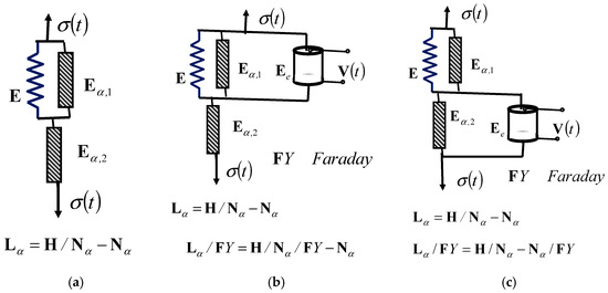
Figure 6.
Three new rheological complex Lethersich–Faraday fractional-type models: (a) structure of the complex linear Lethersich viscoelastic fluid model; (b) structure of the new rheological complex Lethersich–Faraday viscoelastic fluid model; and (c) structure of the new rheological complex Lethersich–Faraday’s elastoviscous solid model.
In Figure 6, three new rheological complex Lethersich fractional-type models, in two variants, are visible. In Figure 6a, the structure of the new Lethersich viscoelastic fluid material model is presented. Figure 6b shows the structure of the new Lethersich–Faraday model of viscoelastic fluid with polarization properties, with Faraday’s element connected in parallel with the Kelvin–Voigt model. Figure 6c shows the structure of the new Lethersich–Faraday-F elastoviscous solid model with polarization properties, with Faraday’s element connected in parallel with Newton’s viscous fluid element.
5.3.1. The Rheological Complex Linear Lethersich–Faraday Model of an Ideal Material with Piezoelectric Properties
This model contains the following parallel-connected elements: Hooke’s element of an ideal elastic material, Newton’s linear element of an ideal viscous fluid, and Faraday’s ideal elastic and piezoelectric element (which form, in parallel connection, the Kelvin–Voigt–Faraday linear model of an ideal material, with the quality of subsequent ecstaticity). They all form a sequential connection with the linear Newtonian element of an ideal viscous fluid. Let us now denote the specific axial deformations and axial dilatations of the Newtonian elements of an ideal viscous fluid in the rheological basic complex linear Kelvin–Voigt–Faraday model of an ideal solid elastoviscous material with piezoelectric properties by and . To establish the total axial dilatation of this new rheological linear Lethersich–Faraday model of an ideal material with piezoelectric properties, which is serially connected in the Kelvin–Voigt–Faraday model with the Newtonian linear element of an ideal viscous fluid, we calculate the sum of these axial dilatations: .
The constitutive relation between the normal stress at the points of the cross-sections of the test tube and the axial dilatations of the linear elements for the rheological complex Lethersich–Faraday linear model of an ideal material with piezoelectric properties is obtained from the relation of the sum of the component velocities of the axial dilatations in the form . For Newton’s model of an ideal linear viscous fluid, the following applies:
Alternatively, for the rheological basic complex Kelvin–Voigt–Faraday ideal model of an ideal solid body with piezoelectric properties, the sum of the dilatations can be calculated as follows:
It follows that the axial dilatation as a function of time can be written in the following form:
in which is the initial axial dilatation of the rheological basic complex Kelvin–Voigt–Faraday ideal linear model of an ideal solid body with piezoelectric properties.
Then, by differentiating in time the previous expression for the axial expansion in Equation (43) of the rheological basic Kelvin–Voigt–Faraday linear model of an ideal body with piezoelectric properties and adding the axial dilatation velocity of the Newtonian linear element of an ideal viscous fluid to the axial dilatation velocity of the rheological basic Lethersich–Faraday ideal linear material model, we obtain the following expression:
Equation (44) represents the differential constitutive relation of the connection between the velocity of axial dilatation and the normal stress of the new rheological complex Lethersich–Faraday linear model of an ideal viscoelastic fluid body with piezoelectric properties.
5.3.2. New Rheological Complex Lethersich–Faraday Model in the Form of Viscoelastic Fluid
The rheological complex fractional-type Lethersich–Faraday model of an ideal material with piezoelectric properties, as shown in Figure 6b, contains the following parallel-connected elements: Hooke’s element of an ideal elastic material, Newton’s fractional-type element of an ideal viscous fluid, and Faraday’s ideal elastic piezoelectric element material (which make up, in parallel connection, a basic fractional-type Kelvin–Voigt–Faraday model of an ideal material with piezoelectric properties and with the quality of subsequent elastity). These elements are in series connection with Newton’s element of an ideal fractional-type viscous fluid.
Let us now denote the specific axial deformations and axial expansions of Newton’s elements of an ideal viscous fluid in the model presented in Figure 6b and in the rheological complex Lethersich–Faraday model of an ideal fractional-type material with piezoelectric properties by and . And for the total axial dilatation of this Lethersich–Faraday model, which is a series connection of the rheological basic complex Kelvin–Voigt–Faraday model of an ideal fractional-type solid body with piezoelectric properties and Newton’s element of an ideal viscous fractional-type fluid, we obtain the sum of these axial expansions and dilatations: .
The differential constitutive relay connection between normal stress and axial dilatations for the rheological complex Lethersich–Faraday model of an ideal fractional-type material with piezoelectric properties is obtained from the relation of the sum of component axial velocities of axial dilatations in the form , that is, the sum of the fractional-type axial dilatation velocities: . For Newton’s element of an ideal viscous fractional-type fluid, the sum can be calculated as follows:
Meanwhile, for the rheological basic complex fractional-type Kelvin–Voigt–Faraday ideal model of an elastoviscous body with piezoelectric properties, the sum of the normal stresses can be calculated as follows:
From this, it follows that the rate of velocity of axial dilatation, of the fractional type, through the rheological basic complex Kelvin–Voigt–Faraday model of an ideal solid material of the fractional type with piezoelectric properties is the solution of an inhomogeneous differential equation of the fractional order, as follows:
Next, let us apply, as in the previous paragraph, the Laplace transform to the previous inhomogeneous differential equation of the fractional order:
On the right-hand side, we have the product of two Laplace transforms of each function, which can be viewed as two functions, which are in convolution. So, we need to determine the inverse transforms of each of those functions individually: and .
The solution of the inhomogeneous differential equation of the fractional order, shown in Equation (47), which describes the axial dilatation through the rheological complex Kelvin–Voigt–Faraday model of an ideal material of the fractional type with piezoelectric properties, is a convolution integral that can be written as follows (see References [64,65,66]):
in which is the initial axial dilatation of the rheological complex Kelvin–Voigt–Faraday ideal model of an ideal visvoelastic fractional-type fluid body with piezoelectric properties.
Then, by differentiating in time the previous expression of axial dilatation shown in Equation (49) of the rheological basic Kelvin–Voigt–Faraday model of an ideal elastoviscous solid body, as well as adding the axial dilatation velocity of the elementary Newtonian element of an ideal fractional-type viscous fluid, to obtain the axial dilatation velocity of the rheological complex Lethersich–Faraday model of an ideal visclastic fluid material, we obtain the following expression:
From the structure, shown in Figure 6b, of the rheological complex Lethersich–Faraday model of this ideal viscoelastic fluid material, which is formed by a series connection of the rheological basic Kelvin–Voigt–Faraday elastoviscous solid material and Newton’s element of an ideal viscous fluid of the fractional type, and from the properties of the models of these ideal materials that we have identified, the first being subsequent elasticity and the second being normal stress relaxation, it can be seen that the rheological complex Lethersich–Faraday material possesses both properties of subsequent elasticity and stress relaxation and that it is a more complex model of the material than its substructures.
The rheological complex Lethersich–Faraday model of an ideal viscoelastic fluid material belongs to the group of rheological viscoelastic creepers.
The new rheological complex Lethersich–Faraday model has one internal degree of freedom of mobility.
5.4. New Rheological Complex Lethersich–Faraday-F Model of an Elastoviscous Solid Material
As we emphasized in the previous Section 5.3, in Figure 6c, the second model of the new rheological complex Lethersich–Faraday-F model of a fractional-type ideal material with piezoelectric properties has the properties of an elastoviscous solid material and has the structural formula . It consists of a regular connection of the rheological basic Kelvin–Voigt model of a fractional-type elastoviscous solid material and the rheological Newton–Faraday model of a fractional-type elastoviscous solid and piezoelectric material with the ability to polarize under deformation and loading.
This rheological model, the second rheological complex Lethersich–Faraday-F model of an ideal elastoviscous solid material, belongs to a group of rheological elastoviscous oscillators.
The second new rheological complex Lethersich–Faraday-F model of an elastoviscous material has one internal degree of freedom of mobility at the point of regular connection of the substructure.
The constitutive relationship of the second rheological complex Lethersich–Faraday model of a fractional-type elastoviscous solid material with piezoelectric properties is determined by the sum of the fractional-type dilatations of the following component substructures: the rheological basic Kelvin–Voigt model of a fractional-type elastoviscous solid material and the rheological Newton–Faraday model of a fractional-type elastoviscous solid of the piezoelectric polarized material. The normal stress through the entire structure of the rheological complex Lethersich–Faraday model of a fractional-type elastoviscous solid material with piezoelectric properties is the same, which means that the resultant normal stress is also the same in the rheological basic complex Kelvin–Voigt model of a fractional-type elastoviscous solid material and in the rheological Newton–Faraday model of a fractional-type elastoviscous solid with piezoelectric properties.
For the rheological Newton–Faraday model, in which they are measured in parallel, the resulting normal stress should be determined as the sum of the normal stresses in the Newton and Faraday models, as follows:
5.5. New Rheological Complex Jeffrey–Faraday Model of a Viscoelastic Fluid Material
In this section, we study the new rheological complex Jeffrey–Faraday model of an ideal fractional-type material with piezoelectric properties, in two variants: 1*—when Faraday’s ideal elastic material with polarization properties is connected in parallel with Hooke’s rheological ideal elastic element, as shown in Figure 7b; and 2*—when Faraday’s ideal elastic material with polarization properties is connected in parallel with the Newton rheological elementary fractional-type viscous fluid element or the rheological basic complex Maxwell viscoelastic fluid model, as shown in Figure 7c. The first case, labeled 1*, is the rheological fractional-type complex Jeffrey–Faraday model of an ideal material with piezoelectric properties, which has the properties of a viscoelastic fluid material and has the structural formula . The second case, labeled 2*, is the rheological fractional-type complex Jeffrey–Faraday model of an ideal material with piezoelectric properties, which has the properties of an elastoviscous solid material and has the structural formula or .
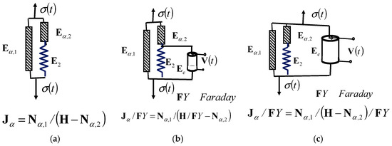
Figure 7.
Three new Jeffrey rheological complex fractional-type models: (a) new Jeffrey viscoelastic fluid model; (b) new Lethersich–Faraday viscoelastic fluid model; (c) new Jeffrey–Faraday-F elastoviscous solid model.
In Figure 7, three new rheological complex Jeffrey fractional-type models, in two variants, are visible. In Figure 7a, the structure of the new rheological complex Jeffrey fractional-type viscoelastic fluid material model is presented. Figure 7b shows the structure of the new rheological complex Jeffrey–Faraday fractional-type model of a viscoelastic fluid with piezoelectric properties, with Faraday’s piezoelectric element connected in parallel with Hooke’s ideal elastic element. Figure 7c shows the new Jeffrey–Faraday elastoviscous solid model, with Faraday’s element connected in parallel with Newton’s fractional-type viscous fluid element.
5.5.1. The Rheological Complex Linear Jeffrey–Faraday Model of an Ideal Material with Piezoelectric Properties
This model contains Hooke’s element of an ideal elastic material and Faraday’s ideal elastic and piezoelectric element connected in parallel, and they are in a sequential connection with the linear Newtonian element of an ideal viscous fluid and in parallel connection with another linear Newtonian element of an ideal viscous fluid. Let us now denote the specific axial deformations and axial dilatations of the linear Newtonian elements of an ideal viscous fluid and the rheological Hooke model of an ideal solid element material by and . And to obtain the total axial dilatation of this new rheological linear complex Jeffrey–Faraday model of an ideal viscoelastic model material with piezoelectric properties, we calculate the sum of these axial dilatations as follows: .
The rheological linear complex Jeffrey–Faraday model of an ideal viscoelastic fluid material with piezoelectric properties, similar to that shown in Figure 7b, contains a parallel connection of Newton’s linear element of an ideal viscous fluid and Maxwell’s model of an ideal viscoelastic material with a parallel connection to Hooke’s ideal elastic model and Faraday’s element of an ideal piezoelectric and ideal elastic material, for which there are individually constitutive relations between normal stress and axial dilatation, i.e., axial dilatation velocity, in the following form:
From here, by integrating Equation (57), the following can be determined:
Then, by adding and , we obtain the resulting normal stress in the rheological linear complex Jeffrey–Faraday model of an ideal viscoelastic fluid material with bolariyation under deformation, shaped by piezoelectric properties, in the following form:
This is measured over the velocity (rate) of axial dilatation as a function of time in the form of Equation (59).
5.5.2. New Rheological Complex Jeffrey–Faraday Model of a Viscoelastic Fluid Material
The new rheological complex Jeffrey–Faraday model of an ideal fractional-type viscoelastic fluid material with piezoelectric properties, as shown in Figure 7b, contains a parallel connection of a Newtonian element of an ideal fractional-type viscous fluid and a new basic complex Maxwell model of an ideal fractional-type viscoelastic material, for which Hooke’s ideal elastic element is connected in parallel to Faraday’s ideal piezoelectric and ideal elastic material elements, which are individually serially connected.
For the first elementary Newtonian element of an ideal fractional-type viscous fluid, the velocity of axial dilatation can be expressed in the following form:
For the second Newtonian element of an ideal fractional-type viscous fluid, in terms of the rate of velocity of fractional-type axial dilatation, the constitutive diferential relation of the element showing the diferential relation between normal stress and velocity rate of axial dilatation, of the fractional order, is in the following form:
For Hooke’s ideal elastic element connected in parallel in the model with Faraday’s ideal piezoelectric and ideal elastic material model, there are individually constitutive relations between normal stress and axial dilatation, i.e., the fractional-type dilatation rate of velocity, which take the following forms:
For Hooke’s element,
For Faraday’s element,
The rates of velocity of the dilatations of the fractional type of these two parallel-connected elements, Hooke’s ideal elastic element and Faraday’s elements of the ideal piezoelectric and ideal elastic material model, are equal, so and the following equation can be formed:
The sum of the normal stresses in parallel elements, i.e., Hooke’s ideal elastic element and Faraday’s element of the ideal piezoelectric and ideal elastic material, can be expressed in the following form:
As such, we have determined through the entire series connection of the structure of new complex Jeffrey–Faraday model of an ideal viscoelastic fluid material, shown in Figure 7b. The velocity of axial dilatation of Newton’s element of viscous fluid, connected in series with the parallel-connected Hooke’s ideal elastic element and Faraday’s ideal piezoelectric model and ideal elastic material model, can be expressed as follows:
Then, the sum of the fractional-type axial dilatation velocity rates of the two parallel elements, Hooke’s element and Faraday’s elastic material, and Newton’s element of an ideal viscous fluid, which is regularly related to them, can be expressed in the following form:
This value is equal to the axial dilatation velocity of the first Newtonian element of an ideal viscous fluid, which is connected in parallel with them, as shown in Figure 7b:
We now determine the normal stress in the first Newtonian viscous fluid element, using the previous velocity of axial dilatation, which we determined using the following equation:
The normal voltage can be expressed in the following form:
Next, we can write a differential constitutive fractional-order relation for the complete rheological complex Jeffrey–Faraday model of an ideal fractional-type viscoelastic fluid material with piezoelectric properties, shown in Figure 7b, which contains a serial connection of a Newtonian element of an ideal fractional-type viscous fluid and a rheological basic complex Maxwell–Faraday model of an ideal fractional-type viscoelastic material with piezoelectric properties, to which Hooke’s ideal elastic element is connected in parallel with the element of Faraday’s ideal piezoelectric and ideal elastic material model with coupled mechanical and electrical fields.
For all those rheological elements of different material properties, we determined the differential constitutive relations individually, on the basis of which we now write that the resulting normal stress of this model is in the form of the sum of the component normal stresses in the parallel branches of the complex Jeffrey–Faraday model of an ideal viscoelastic fluid material, shown in Figure 7b, in the following form:
The preceding constitutive relation shown in Equation (74) is in the form of an inhomogeneous differential relation of fractional-order exponent , where . From the previous relation, we form an ordinary inhomogeneous fractional differential equation of the following form:
It gives the relation between the dilatation of Hooke’s element and the resulting normal stress in the structure of the complex Jeffrey–Faraday model of an ideal viscoelastic fluid material, shown in Figure 7b, which can also be written in the following form:
From this, it can be determined that
because
in which is the axial dilatation of the elements. Next, we need to determine the solutions of this inhomogeneous ordinary differential equation of the fractional order which is in the following form, adapted from Equation (77):
Alternatively, it can be transformed as follows:
Using Equation (77), the inhomogeneous differential equation of fractional-order exponent is solved by applying the Laplace transform, then developing it in a degrees series and then returning it, with the inverse Laplace transform, as follows:
Then, the following can be determined:
At constant axial dilatation of the rheological complex Jeffrey–Faraday model of an ideal viscoelastic fluid material, relaxation of normal stress occurs.
The new rheological complex Jeffrey–Faraday model has one internal degree of freedom of mobility.
5.6. New Rheological Complex Jeffrey–Faraday Model as an Elastoviscous Solid Material
In this section, we study the second variant of the new rheological complex Jeffrey–Faraday-F model of an ideal elastoviscous fractional-type solid material with piezoelectric properties, when Faraday’s ideal elastic element with polarization properties is connected in parallel with the rheological fractional-type Newtonian viscous fluid element or the rheological basic complex Maxwell viscoelastic fluid model, as shown in Figure 7c. As we wrote in this case, it is the rheological complex Jeffrey–Faraday model of a fractional-type ideal material with piezoelectric properties, which has the properties of an elastoviscous solid material and has the structural formula or .
The rheological complex Jeffrey–Faraday model of a fractional-type elastoviscous solid and piezoelectric material has the ability to polarize under deformation and loading.
This rheological model, the second rheological complex Jeffrey–Faraday-F model of an ideal elastoviscous solid material, belongs to a group of rheological elastoviscous oscillators.
The second new rheological complex Jeffrey–Faraday-F model has one internal degree of freedom of mobility at the point of regular connection in its substructure.
The constitutive relation of the second rheological complex Jeffrey–Faraday-F model of an elastoviscous solid material is easily determined by the sum of the component normal stresses of two elementary rheological elements connected in parallel in a basic complex model: the Newtonian ideal viscous fluid element and the Faraday element in one rheological basic complex Maxwell model of an elastoviscous fluid, as shown in Figure 7c.
The normal stress through the entire structure of the rheological complex Jeffrey–Faraday-F model of an elastoviscous solid material is the resultant normal stress of the components:
The normal stress at the points of the cross-section is the same throughout the entire modified Maxwell model , so we can write the constitutive relations of each basic rheological element in this series connection; as such, the normal stresses in the dilatation function are
The velocity rate of axial dilatation of the fractional-type rheological basic complex Maxwell model , the fractional-type equal to the sum of the dilatation rates, the fractional-type Newtonian viscous element , and Hooke’s ideal elastic element can be expressed in the following form:
From this, it can be determined that and therefore and . As such, it follows that a sum (see Figure 7c) can be used for axial dilatation analysis:
This model has the property of subsequent elasticity, and the structure model of the rheological complex Jeffrey–Faraday-F model of an elastoviscous solid material in the substructure of the basic complex Maxwell model exhibits normal stress relaxation. The structure of the rheological complex Jeffrey–Faraday-F model of an elastoviscous solid material has the property of subsequent elasticity.
This rheological model, the second rheological complex Jeffrey–Faraday-F model of an ideal elastoviscous solid material, belongs to the group of rheological elastoviscous oscillators.
The second new rheological complex Jeffrey–Faraday model of a fractional-type elastoviscous material with piezoelectric properties has one internal degree of freedom of mobility at the point of regular connection in its substructure.
5.7. New Rheological Complex Burgers–Faraday Model of a Viscoelastic Fluid Material
In this section, we study two new rheological complex Burgers–Faraday models of an ideal fractional-type material with piezoelectric properties: 1*—when Faraday’s ideal elastic element with polarization properties is connected in parallel with the rheological basic complex Kelvin–Voigt ideal elastoviscous fluid model, as shown in Figure 8b; and 2*— when Faraday’s ideal elastic element with polarization properties is connected in parallel with the rheological basic complex Maxwell viscoelastic fluid model, as shown in Figure 8c. The first case, labeled 1*, is the rheological complex Burgers–Faraday model of an ideal material, which has the properties of a viscoelastic fluid material and has the structural formula , .
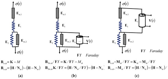
Figure 8.
Three new rheological complex Burgers fractional-type models: (a) new complex Burgers viscoelastic fluid model; (b) new complex Burgers–Faraday fractional-type viscoelastic fluid model with piezoelectric properties; (c) new complex Burgers–Faraday-F elastoviscous solid model with piezoelectric properties.
The second case, labeled 2*, is the rheological complex Burgers–Faraday-F model of an ideal material, which has the properties of an elastoviscous solid material and has the structural formula , ; see Figure 8c.
In Figure 8, the structures of three new rheological complex Burgers models, one Burgers model as well as two Burgers–Faraday models, are presented. Figure 8a shows a new complex Burgers fractional-type viscoelastic fluid model. Figure 8b shows a new complex Burgers–Faraday viscoelastic fluid material model. In Figure 8c, a new complex Burgers–Faraday-F elastoviscous solid material model is visible.
The second rheological complex Burgers–Faraday model of an ideal viscoelastic fluid material with piezoelectric properties is shown in Figure 8b, and represents a series connection of the rheological basic complex Maxwell viscoelastic fluid model and the rheological basic complex Kelvin–Voight–Faraday elastoviscous solid model (with a piezoelectric element connected in parallel with the Faraday element). Both rheological basic complex models are of the fractional type; one is formed of an ideal viscoelastic fluid and the second of elastoviscous solid materials.
The structural formula of the Burgers–Faraday viscoelastic fluid material is in the form .
The third rheological complex Burgers–Faraday model of an ideal elastovisous solid material with piezoelectric properties is shown in Figure 8c, and represents a series connection of the rheological basic complex Maxwell–Faraday elastoviscous solid model (with a piezoelectric element connected in parallel with the Faraday element) and the rheological basic complex Kelvin–Voight elastoviscous solid model. Both rheological basic complex models are of the fractional type, and both utilize ideal and different viscoelastic solid material models. The constitutive relations (equations of coupled mechanical normal stress and axial expansions) of this rheological complex material model are now easily determined using the following structural formula: .
5.7.1. New Rheological Complex Burgers–Faraday Linear Model of a Linear Viscoelastic Fluid Material with Piezoelectric Properties
First, we will study the properties of the new rheological complex Burgers–Faraday linear model of a linear viscoelastic fluid material with piezoelectric properties, which has a structure similar and analogous to the structure of the model shown in Figure 8b, in which the Newton elements are linear.
The total axial dilatation of the complex linear-type Burgers–Faraday viscoelastic fluid model of an ideal material with piezoelectric properties is equal to the sum of the component axial dilatations , , and , of the component substructure, as well as the basic complex Maxwell and Kelvin–Voigt–Faraday models (complex model with Faraday’s element connected in parallel). The mechanical normal stress in all of the cross-sections of the component substructures of the basic complex models is the same throughout the entire complex Burgers–Faraday model. Based on this analysis and these derived conclusions, we can determine the following:
Let us differentiate the first constitutive relation shown in Equation (89) from the previous system, and replace the terms from the third constitutive equation of the previous system given in Equations (90) and (91); based on that, we can write the following constitutive relation for the complex Burgers–Faraday linear model of an ideal viscoelastic fluid material:
Next, the last constitutive relation shown in Equation (92) can be differentiated once more in time to obtain the following:
Let us now multiply Equation (90) by and Equation (94) by and combine them with for the component Kelvin–Voigt–Faraday complex model of an ideal material with piezoelectric properties so that we obtain the following relation:
Finally, we obtain the following differential relationship between the mechanical normal stress and the first and third derivatives by time of the axial dilatation in the following form:
5.7.2. New Rheological Complex Burgers–Faraday Model of a Fractional-Type Viscoelastic Fluid Material
The rheological complex Burgers–Faraday model of an ideal viscoelastic fluid material is shown in Figure 8b, and represents, as we explain, a series connection of the rheological basic complex Maxwell viscoelastic fluid material model and the rheological basic complex Kelvin–Voight–Faraday elastoviscous solid material model (with a Faraday piezoelectric element connected in parallel). Both rheological basic complex models are of the fractional type, and utilize ideal viscoelastic fluids as well as elastoviscous solid materials. The constitutive relations are differential equations of the fractional order of coupled mechanical normal stress and axial expansions. The structural formula of this rheological complex material model is expressed in the following form: , .
The constitutive relations (equations of relation between normal stress and axial dilatation) of this complex material model, a modified Burgers–Faraday model of an ideal fractional-type material with piezoelectric properties, contain derivatives of the fractional-order exponent , where , by time.
The total axial dilatation of the rheological complex Burgers–Faraday ideal fractional-type viscoelastic fluid material model with the piezoelectric properties of an ideal material is equal to the sum of the component axial dilatations , , and of the component substructure, as well as the rheological complex basic models: the rheological basic complex Maxwell and the rheological basic complex Kelvin–Voigt–Faraday models (complex model with a parallel-connected Faraday ideal elastic element with piezoelectric properties). Mechanical normal stresses in all cross-sections of the component substructure of the basic complex models are equal throughout the entire rheological complex Burgers–Faraday viscoelastic fluid model: . Based on this analysis and the derived conclusions, we can determine the following relations:
Let us differentiate the first constitutive relation using the differential operator of fractional-order exponent , , from the previous system, as shown in Equation (98), and replace the terms from the third constitutive formula in Equation (99) of the previous system; based on that, we could write the constitutive relation for the rheological complex Burgers–Faraday model of an ideal viscoelastic fluid material in the following form:
or
As throughout the viscoelastic fluid model structure , the normal stress is equal to , the previous two equations of the fractional order can be expressed as follows:
These last two relations between normal stress and axial dilatation are coupled differential constitutive relations of the fractional-order exponent of the structure model of the ideal rheological viscoelastic fluid material model, which is shown in Figure 8b.
To repeat, of the ideal viscoelastic fluid material with piezoelectric properties, with the fractional-derivative-order exponent , where , represents the regular serial connection of the Maxwell and Kelvin–Voight–Faraday models, both rheological complex fractional-type models of an ideal material with piezoelectric properties, one utilizing a viscoelastic fluid and the second an elastoviscous solid, and in regular sequential conection gives the final results for the viscoelastic fluid material model. And under certain conditions, of the ideal viscoelastic fluid material with piezoelectric properties, with fractional-derivative-order exponent , where , has properties of subsequent elasticity and/or relaxation of normal stress in its substructure.
From this system, expressed in Equations (102) and (103), of differential constitutive relations of the fractional-order exponent , where , we can eliminate the velocity of dilatation of this fractional type and obtain only one differential constitutive relation highlighting the connection between the normal stress and axial dilatation of the structure of the rheological complex Burgers–Faraday model of an ideal fractional-type viscoelastic fluid material with piezoelectric properties in the domain of the Laplace transform, as follows:
Next, let us integrate the second equation, Equation (105), into the first equation, Equation (104), to obtain one relation:
And next, by applying the inverse Laplace transform in Equation (106), it is possible to obtain the convolutional integral and the time function of the normal stress from the axial dilatation of the structure for the rheological complex Burgers–Faraday model of an ideal fractional-type material with piezoelectric properties.
This rheological model, the second rheological complex Burgers–Faraday-F model of ideal viscoelastic fluid material, belongs to a group of rheological viscoelastic creepers.
The second new rheological complex Burgers–Faraday model of a fractional-type viscoelastic fluid material with piezoelectric properties has two internal degrees of freedom of mobility at the points of regular connection in its substructure.
5.8. Second New Rheological Complex Burgers–Faraday-F Model of an Elastoviscous Solid Material
Next, we will analyze the constitutive relations of the substructure of the second new complex Burgers–Faraday-F model of an elastoviscous solid material, when a Faraday element is connected in parallel to the substructure of a basic complex Maxwell model.
Along the entire substructure of the complex Maxwell model, the normal stress is the same, and the velocity of axial dilatation in individual regularly connected elements can be expressed as follows: in the Hooke element, it is , i.e., , while in the Newton element of a fractional-type fluid, it is . The total velocity of axial dilatation in the substructure of the Maxwell viscoelastic material can now be expressed in the following form:
If we apply the Laplace transform to the previous differential constitutive relations expressed in Equations (107) and (119) of the fractional-order exponent , where , we obtain the following:
We obtained the previous relationship shown in Equation (110) as the relationship between the Laplace transform of the axial dilatation in the Maxwell model and the Laplace transform of the normal stress in that model, which is a substructure of the complex Burgers–Faraday-F model.
The fractional-type axial dilatation velocity in a parallel-connected Faraday element with Maxwell’s model is expressed in the following form:
Next, using the previous differential constitutive relationship demonstrated in Equation (111), of the fractional-order exponent , where , it can be determined that , in a substructure consisting of a Faraday element connected in parallel with a Maxwell model, which together form the substructure of the complex Burgers–Faraday-F model, is equal to
If we apply the Laplace transform to the previous constitutive relation of the fractional order, we obtain the following:
We obtained the previous expression as the relationship between the Laplace transform of the normal stress in a Faraday element with piezoelectric properties, connected in parallel with the rheological basic complex Maxwell model of the fractional type, and the Laplace transform of the normal stress in the Maxwell model, which is a substructure of the complex Burgers–Faraday-F model.
The total normal stress in the Maxwell–Faraday model, which contains a parallel-connected Faraday element, which is a substructure of the complex Burgers–Faraday-F model, can be expressed as follows:
If we apply the Laplace transform to the previous constitutive relationship expressed in Equation (114), using the fractional-order exponent , where , we obtain the following:
We obtained the previous expression as the relationship between the Laplace transform of in the basic complex Maxwell–Faraday elastoviscous solid model, which contains a parallel-connected Faraday element, which is a substructure of the complex Burgers–Faraday-F model, and the Laplace transform of in the basic Maxwell–Faraday model.
Next, we use the knowledge that the substructure of the complex Burgers–Faraday-F elastoviscous solid material consists of the order of two substructures—the structure of the basic complex Maxwell–Faraday elastoviscous solid material model and the substructure consisting of the solid material—and we write the following differential constitutive relations of fractional-order exponent , where :
Next, we establish the following system, including the differential constitutive relations of the fractional-order exponent , where , of the complex Burgers–Faraday-F elastoviscous solid material model in the following form:
These differential constitutive relations of fractional-order exponent , where , as shown in Equations (119)–(124), give the relationships of axial dilatation and normal stress for the complex Burgers–Faraday-F elastoviscous solid material, as well as the normal stresses and axial dilatations in the substructures of the basic complex Kelvin–Voigt elastoviscous solid material and the basic complex Maxwell–Faraday elastoviscous solid material.
If we apply the Laplace transform to the previous two differential constitutive relations of fractional-order exponent , where , as shown in Equations (129)–(124), we obtain the following relations:
These differential constitutive relations of the fractional-order exponent , where , give the connections between the Laplace transformations of the normal stress and the Laplace transformations of the axial dilatation of the complex Burgers–Faraday-F elastoviscous solid material, and the axial dilatations , namely , and the normal stresses , namely , in the substructures of the basic complex Kelvin–Voigt elastoviscous solid material and the basic complex Maxwell–Faraday elastoviscous solid material.
This new model, the second complex Burgers–Faraday-F model of an ideal elastoviscous solid material, belongs to a group of rheological elastoviscous oscillators.
The second new complex Burgers–Faraday-F model, has two internal degrees of freedom of mobility at the points of regular connections in its substructures.
6. Discussion
Based on the derived differential constitutive relations, differential equations, fractional-order calculations, Laplace transformations, dynamics of the rheological complex material models, and approximate analytical solutions, as well as the attached properties of the structures and models and our analysis of them, in our final considerations, we define a number of conclusions in the form of theorems. These theorems are as follows:
Theorem 1.
From the structural scheme of the rheological complex models, we can identify the differences between the types of models, and it is therefore possible to divide the rheological complex models into two groups. The first group is a group of rheological elastoviscous solid bodies with the potential to oscillate and the other is a group of fractional-type rheological viscoelastic fluid materials with the potential to creep.
Theorem 2.
If at least one of Newton’s viscous fluid elements, of the fractional type, is regularly serially connected in the structure independently, and is not in parallel connection or part of another parallel connection with any Hooke ideal elastic elements or Faraday ideal elastic piezoelectric elements in a complex rheological model, then it has the model and structure of a viscoelastic fluid material. In this case, the electrical voltage of the Faraday element changes according to the creep dynamics.
Theorem 3.
If each of Newton’s viscous fluid elements, of the fractional type, is connected in a parallel or intra-parallel connection with one of Hooke’s ideal elastic elements or Faraday’s ideal elastic and piezoelectric elements, then the rheological complex material model is an elastoviscous solid material model, with the potential to oscillate. In this case, the electric voltage of the Faraday element oscillates.
Theorem 4.
Each regular connection of one of Newton’s fluid elements, of the fractional type, introduces one internal degree of freedom of movement in the complex rheological model, in addition to the external degrees of freedom of movement present in complex rheological models.
Theorem 5.
Basic rheological complex models are constructed from at least two rheological models connected in parallel or in series. These are basic complex models that belong to the class of fractional-type models and have piezoelectric properties, and include the rheological basic complex Kelvin–Voigt–Faraday model in parallel connection with three rheological elements and the rheological basic complex Maxwell–Faraday model in series connection with three serially connected rheological elements.
Theorem 6.
The rheological basic complex Kelvin–Voigt–Faraday model, which is in parallel connection with three rheological elements, is a fractional-type model of an elastoviscous solid material with piezoelectric properties and the property of subsequent elasticity.
The rheological basic complex Maxwell–Faraday model, which is in series connection with three serially connected rheological elements, is a fractional-type model of a viscoelastic fluid material with piezoelectric properties and the property of normal stress relaxation.
Table 1 shows a tabular comparative overview of this new class of complex rheological models of the fractional type of ideal materials with piezoelectric properties. In the vertical columns of Table 1, rheological complex models of elastoviscous solid materials and rheological complex models of fractional-type viscoelastic fluid materials with piezoelectric properties are compared. In the first row of Table 1, the basic rheological complex Kelvin–Voigt–Faraday and Maxwell–Faraday models are shown, which contain the same three basic rheological elements: in the first model, they are all in a parallel coupling, and in the second model, they are all in a series coupling. In the other horizontal rows of Table 1, other rheological complex models are compared in pairs containing the same rheological elements in terms of number and properties, but in which the type of material model is changed by parallel attachment of the Faraday element to another substructure in the model, from elastoviscous solid to viscoelastic fluid materials.

Table 1.
Tabular comparative overview of a new class of complex rheological models of the fractional type of ideal materials with piezoelectric properties.
7. Concluding Considerations
For each rheological model from the newly introduced class of rheological complex fractional-type material models with piezoelectric polarization properties, whose dynamics we have studied and presented in the previous sections, we can introduce the assumption that these are standard light models, which are of negligible mass, but with the properties of possessing potential energy and polarization during mechanical deformations and dissipating mechanical energy due to the fractional-type axial dilatation rate. Then, we can use these standard light rheological models of the fractional type with piezoelectric properties as models of rigid body binding in rheological discrete dynamic systems and consider the dynamics of newly created rheological discrete dynamic systems, which will be explained in more detail in the following works (see References [1,2,3]).
Rheological complex models of elastoviscous and viscoelastic fractional-type materials with polarized piezoelectric properties of various substances are of interest due to the widespread use of viscoelastic–plastic bodies under loading.
In this paper, new standard light complex rheological models of ideal fractional-type materials with piezoelectric properties are obtained by parallel or serial binding of basic complex rheological fractional-type models with rheological ideal elastic Faraday elements with piezoelectric properties.
The rheological Faraday element, which is an ideal elastic element and has ideal piezoelectric properties, is a rheological element with a coupled mechanical and electric field, and has the properties of polarization when it is deformed in the area of elastic deformation under the external action of load.
In this paper, we presented a large number of completely new scientific results about rheological complex material models and gave important ideas and theoretical foundations for further research into the properties of these rheological discrete dynamic systems of the fractional order with piezoelectric properties.
In addition, we have opened a wide field for further research into the properties of rheological discrete dynamic systems with many degrees of freedom of movement, both discrete and continuous systems of the fractional type and with coupled mechanical and piezoelectric fields. We have laid the fundamental foundations and presented ideas for those studies.
In the end, we can emphasize that all structural formulas of rheological complex models of substances are assembled analogously, like those in chemistry or those of complex electric circuits. Analogies, written by the founder of the Serbian School of Mathematics, Mihailo Pćetrović, one of the three doctoral students of well-known French scientist Julius Henri Poicare in References [67,68,69,70,71], enabled the transfer of acquired knowledge from one scientific field to another.
A new direction of research into the dynamics of the newly introduced class of rheological models of fractional-type materials with piezoelectric properties in non-isothermal conditions has been suggested. This is a very important direction of research for future projects.
In this work, we used analytical methods and analytical approaches, but researchers have access to new modern numerical methods and commercial software that can be used to study the dynamics of rheological discrete dynamic systems with a finite number of degrees. These can be used to solve systems of differential equations of the fractional order, including those with nonlinearities, and to study the phenomena of nonlinear rheological oscillations of the fractional type with piezoelectric properties, or nonlinear rheological creepers of the fractional type with piezoelectric properties.
The manuscript presents the differential constitutive relations of the fractional type for each of the new rheological complex models of materials of the fractional type with piezoelectric properties. Both of them present a mathematical description and represent the validation of each of the models. Validation can also be experimental, and the author is convinced that the theoretical results presented in the paper will inspire experimenters to experimentally validate the theoretical results.
At the end, the paper presents the basic principles of connecting rheological elements into basic complex and more complex material models. It is shown that rheological models can be connected in parallel and in series. It is also shown by decomposition of basic complex models that differential constitutive relations of the fractional order can be composed using the sum of component normal stresses for parallel-connected elements or the sum of axial dilatations for regularly connected elements. These two approaches can be used to construct more complex hybrid rheological material models.
Funding
This research received no external funding.
Data Availability Statement
The original contributions presented in this study are included in the article. Further inquiries can be directed to the corresponding author.
Acknowledgments
The author would like to thank the reviewers and the Assistant Editor for their useful comments and suggestions that improved the quality of the manuscript.
Conflicts of Interest
The author declares no conflicts of interest.
References
- Hedrih, R.K. Izabrana Poglavlja Teorije Elastičnosti (Selected Chapters of Theory of Elasticity); Prošireno i Dopunjeno izdanje; Mašinski Fakultet u Nišu: Niš, Serbia, 1988; p. 425. Available online: http://elibrary.matf.bg.ac.rs/handle/123456789/3766?show=full (accessed on 5 December 2024).
- Hedrih, K.S.; Machado, J.T. Discrete fractional order system vibrations. Int. J. Non-Linear Mech. 2015, 73, 2–11. [Google Scholar] [CrossRef]
- Hedrih, K.R.; Hedrih, A.N. The Kelvin–Voigt visco-elastic model involving a fractional-order time derivative for modelling torsional oscillations of a complex discrete biodynamical system. Acta Mech. 2023, 234, 1923–1942. [Google Scholar] [CrossRef]
- Hedrih, K.R.; Milovanovic, G.V. Elements of mathematical phenomenology and analogies of electrical and mechanical oscillators of the fractional type with finite number of degrees of freedom of oscillations: Linear and nonlinear modes. Commun. Anal. Mech. 2024, 16, 738–785. [Google Scholar] [CrossRef]
- Hedrih, K.R.; Hedrih, A.N. Rheological Burgers–Faraday Models and Rheological Dynamical Systems with Fractional Derivatives and Their Application in Biomechanics. Fractal Fract. 2024, 8, 742. [Google Scholar] [CrossRef]
- Zorica, D.M.; Cveticanin, S.M. Dissipative and generative fractional RLC circuits in the transient regime. Appl. Math. Comput. 2023, 459, 128227. [Google Scholar] [CrossRef]
- Jelic, S.Z.; Zorica, D.M. Energy balance for fractional anti-Zener and Zener models in terms of relaxation modulus and creep compliance. Appl. Math. Model. 2023, 123, 688–728. [Google Scholar] [CrossRef]
- Zorica, D.; Oparnica, L. Energy dissipation for hereditary and energy conservation for non-local fractional wave equations. Philos. Trans. R. Soc. A-Math. Phys. Eng. Sci. 2020, 378, 20190295. [Google Scholar] [CrossRef] [PubMed]
- Zorica, D.M.; Atanackovic, T.M.; Vrcelj, Z.; Novakovic, B. Dynamic Stability of Axially Loaded Nonlocal Rod on Generalized Pasternak Foundation. J. Eng. Mech. 2017, 143, D4016003. [Google Scholar] [CrossRef]
- Rabotnov, Y.N. Creep Problems in Structural Members; Series in Applied Mathematics and Mechanics; North-Holland Publishing: Amsterdam, The Netherlands, 1969. [Google Scholar]
- Escalante-Martínez, J.E.; Gómez-Aguilar, J.F.; Calderón-Ramón, C.; Morales-Mendoza, L.J.; Cruz-Orduna, I.; Laguna-Camacho, J.R. Experimental evaluation of viscous damping coefficient in the fractional underdamped oscillator. Adv. Mech. Eng. 2016, 8, 1687814016643068. [Google Scholar] [CrossRef]
- Gómez-Aguilar, J.F.; Yépez-Martínez, H.; Calderón-Ramón, C.; Cruz-Orduña, I.; Escobar-Jiménez, R.F.; Olivares-Peregrino, V.H. Modeling of a mass-spring-damper system by fractional derivatives with and without a singular kernel. Entropy 2015, 17, 6289–6303. [Google Scholar] [CrossRef]
- Gómez-Aguilar, J.F. Analytic solutions and numerical simulations of mass-spring and damperspring systems described by fractional differential equations. Rom. J. Phys. 2015, 60, 311–323. [Google Scholar]
- Gómez-Aguilar, J.F.; Rosales, J.J.; Bernal, J.J. Mathematical modelling of the massspring-damper system—A fractional calculus approach. Acta Univ. 2012, 22, 5–11. [Google Scholar] [CrossRef]
- Gómez-Aguilar, J.F.; Rosales-García, J.J.; Bernal-Alvarado, J.J.; Córdova-Fraga, T.; Guzmán-Cabrera, R. Fractional mechanical oscillators. Rev. Mex. FCA 2012, 58, 348–352. [Google Scholar]
- Miličić, I.M.; Vlajić, L.M. Models of Civil Engineering–Classification and Definition, Conference Paper, Conference DQM-2006, Belgrade. Available online: https://www.researchgate.net/publication/289098053/ (accessed on 5 December 2024).
- Tomović, Z. Reološki model puzanja matriksa meke stijene (Rheologica model od of soft rocks of creep). Mater. I Konstr. 2007, 50, 3–19. [Google Scholar]
- Oldham, K.B.; Spanier, J. The Fractional Calculus; Academic Press: New York, NY, USA, 1974. [Google Scholar]
- Ross, B. A brief history and exposition of the fundamental theory of fractional calculus. In Fractional Calculus and Its Applications: Proceedings of the International Conference Held at the University of New Haven, June 1974; Springer: Berlin/Heidelberg, Germany, 2006; pp. 1–36. [Google Scholar] [CrossRef]
- Miller, K.S.; Ross, B. An Introduction to the Fractional Calculus and Fractional Differential Equations; Wiley: New York, NY, USA, 1993. [Google Scholar]
- Letnikov, A.V. Theory of differentiation with an arbitrary index. Mat. Sb. 1868, 3, 1–66. [Google Scholar]
- Letnikov, A.V. An explanation of the concepts of the theory of differentiation of arbitrary index. Mat. Sb. 1872, 6, 413–445. [Google Scholar]
- Samko, S.G.; Kilbas, A.A.; Marichev, O.I. Fractional Integrals and Derivatives–Theory and Applications; Gordon and Breach Science Publishers: Amsterdam, The Netherlands, 1993. [Google Scholar]
- Das, S. Functional Fractional Calculus; Springer: Berlin/Heidelberg, Germany, 2011. [Google Scholar] [CrossRef]
- Debnath, L. A brief historical introduction to fractional calculus. Int. J. Math. Educ. Sci. Technol. 2004, 35, 487–501. [Google Scholar] [CrossRef]
- Machado, J.T.; Kiryakova, V.; Mainardi, F. Recent history of fractional calculus. Commun. Nonlinear Sci. Numer. Simulat. 2011, 16, 1140–1153. [Google Scholar] [CrossRef]
- Kilbas, A.A.; Srivastava, H.M.; Trujillo, J.J. Theory and Applications of Fractional Differential Equations; Elsevier: Amsterdam, The Netherlands, 2006. [Google Scholar]
- Mainardi, F. Fractional Calculus and Waves in Linear Viscoelasticity. An Introduction to Mathematical Models; Imperial College Press: London, UK, 2010. [Google Scholar] [CrossRef]
- Podlubny, I. Fractional Differential Equations; Academic Press: New York, NY, USA, 1999. [Google Scholar]
- Kiryakova, V. A brief story about the operators of generalized fractional calculus. Fract. Calc. Appl. Anal. 2008, 11, 203–220. [Google Scholar]
- Herrmann, R. Fractional Calculus—An Introduction for Physicists; World Scientific: Singapore, 2014. [Google Scholar] [CrossRef]
- Kiryakova, V. Generalized Fractional Calculus and Applications; Pitman Research Notes I Mathematics Series, 301; Longman Scientific & Technical: Harlow, UK, 1994. [Google Scholar]
- Diethelm, K. The Analysis of Fractional Differential Equations; Springer: Berlin/Heidelberg, Germany, 2010. [Google Scholar] [CrossRef]
- Sandev, T.; Tomovski, Ž. Fractional Equations and Models. Theory and Applications; Springer: Cham, Switzerland, 2019. [Google Scholar] [CrossRef]
- Li, C.; Zeng, F. Numerical Methods for Fractional Calculus; CRC Press: Boca Raton, FL, USA, 2015. [Google Scholar] [CrossRef]
- Baleanu, D.; Diethelm, K.; Scalas, E.; Trujillo, J.J. Fractional Calculus: Models and Numerical Methods; World Scientific: Singapore, 2012. [Google Scholar]
- Wolfram, S. The Mathematica Book; Wolfram Media, Inc.: Champaign, IL, USA, 2003. [Google Scholar]
- Esmaeili, S.; Shamsi, M.; Luchko, Y. Numerical solution of fractional differential equations with a collocation method based on M¨untz polynomials. Comput. Math. Appl. 2011, 62, 918–929. [Google Scholar] [CrossRef]
- Atanacković, T.; Pilipović, S.; Stanković, B.; Zorica, D. Fractional Calculus with Applications in Mechanics: Vibrations and Diffusion Processes; Wiley-ISTE: London, UK, 2014. [Google Scholar]
- Atanacković, T.; Pilipović, S.; Stanković, B.; Zorica, D. Fractional Calculus with Applications in Mechanics: Wave Propagation, Impact and Variational Principles; Wiley-ISTE: London, UK, 2014. [Google Scholar]
- Garrappa, R.; Popolizio, M. Evaluation of generalized Mittag-Leffler functions on the real line. Adv. Comput. Math. 2013, 39, 205–225. [Google Scholar] [CrossRef]
- Gorenflo, R.; Loutchko, J.; Luchko, Y. Computation of the Mittag-Leffler function and its derivatives. Fract. Calc. Appl. Anal. 2002, 5, 491–518. [Google Scholar]
- Luo, M.J.; Milovanovi´c, G.V.; Agarwal, P. Some results on the extended beta and extended hypergeometric functions. Appl. Math. Comput. 2014, 248, 631–651. [Google Scholar] [CrossRef]
- Mitrinović, D.S.; Djoković, D.Ž. Special Functions (Specijalne Funkcije); Gradjevinska Knjiga: Beograd, Serbia, 1964; p. 267. [Google Scholar]
- Novati, P. Numerical approximation to the fractional derivative operator. Numer. Math. 2014, 127, 539–566. [Google Scholar] [CrossRef]
- Milovanovic, G.V.; Rathie, A.K. On a quadratic transformation due to Exton and its generalization. Hacet. J. Math. Stat. 2019, 48, 1706–1711. [Google Scholar] [CrossRef]
- Milovanović, G.V.; Rathie, A.K.; Vasović, N.M. Summation identities for the Kummer confluent hypergeometric function 1F1(a; b; z). Kuwait J. Sci. 2023, 50, 190–193. [Google Scholar] [CrossRef]
- Perić, L. Spregnuti Tenzori Stanja Piezoeletričnih Materijala (Coupled Tensors of the Piesoelectric Material States). Ph.D. Thesis, Faculty of Mechanical Engineering in Niš, Niš, Serbia, 2005. (In Serbian). [Google Scholar]
- Hedrih, K.S.; Babović, V.; Šarković, D. An auxi liary size distribution model for the ultrasonically produced water droplets. In Experimental Thermal and Fluid Science–ETF; Elsevier: Amsterdam, The Netherlands, 2006; Volume 30, pp. 559–564. [Google Scholar] [CrossRef]
- Thomas, J.M. Michael Faraday and The Royal Institution: The Genius of Man and Place (PBK); CRC Press: Boca Raton, FL, USA, 1991; ISBN 978-0-7503-0145-9. [Google Scholar]
- Thompson, S. Michael Faraday, His Life and Work; Cassell and Company: London, UK, 1901; ISBN 978-1-4179-7036-0. [Google Scholar]
- Đurić, M. Teorija Spregnutih i Prethodno Napregnutih Konstrukcija, SANU, (Theory of Coupled and Prestressed Construction); Serbian Academy of Science and Arts, Bool (SANU): Beograd, Serbia, 1963. [Google Scholar]
- Mihailović, V.; Landović, A. The Relation Properties of Concrete and Their Characteristic in Rheological Models; ZBORNIK RADOVA 19; Univerzitet u Novom Sadu, GraĊevinski Fakultet Subotici: Subotica, Serbia, 2010. [Google Scholar]
- Stoiljkoic, D.T. Rheological modeling of yarn elongation. Tekstil 2007, 56, 554–561. [Google Scholar]
- Stoiljkoic, D.T. Dinamicko Ponasanje Sistema Mehanizam–Radni Objekat Tkackog Procesa. Ph.D. Thesis, Masinski Fakultet u Nišu, Niš, Serbia, 1992. [Google Scholar]
- Yang, X.-J. New rheological problems involving general fractional Derivatives with nonsingular power-law kernels. Proc. Rom. Acad. Ser. A 2018, 19, 45–52. [Google Scholar]
- Yang, X.; Chen, W.; Xiao, R.; Ling, L. A Fractional Model for Time-Variant Non-Newtonian Flow. Therm. Sci. 2017, 21, 61–68. [Google Scholar] [CrossRef]
- Verdier, C. Review: “Rheological properties of living materials. From cells to tissues”. J. Theor. Med. 2003, 5, 67–91. [Google Scholar]
- Bonfanti, A.; Fouchard, J.; Khalilgharibi, N.; Charras, G.; Kabla, A. A unified rheological model for cells and cellularised materials. R. Soc. Open Sci. 2020, 7, 190920. [Google Scholar] [CrossRef] [PubMed]
- Dabiri, D.; Saadat, M.; Mangal, D.; Jamali, S. Fractional rheology-informed neural networks for data-driven identification of viscoelastic constitutive models. Rheol. Acta 2023, 62, 557–568. [Google Scholar] [CrossRef]
- Fabrizio, M. Fractional rheological models for thermomechanical systems. Dissipation and free energies. Fract. Calc. 2014, 17, 206–223. [Google Scholar] [CrossRef]
- Goroško, O.A.; Hedrih, K. Analitička Dinamika (Mehanika) Diskretnih Naslednih Sistema, (Analytical Dynamics (Mechanics) of Discrete Hereditary Systems); University of Niš: Niš, Serbia, 2001; p. 426. ISBN 86-7181-054-2. (In Serbian) [Google Scholar]
- Hedrih, K.R. Generalized Function of Fractional Order Dissipation of System Energy and Extended LAGRANGE Differential Lagrange Equation in Matrix Form; Dedicated to 86th Anniversary of Radu MIRON’S Birth; Kawaguchi Institute of Mathematics Society: Kawaguchi, Japan, 2014; Volume 75, pp. 35–51. [Google Scholar]
- Bačlić, B.S.; Atanacković, T.M. Stability and creep of a fractional derivative order viscoelastic Rod. In Bulletin T, CXXI de L’Academie Serbe des Sciences st de Arts-2000; Class des Sciences Mathematques et Naturelles Sciences Mathematiques; L’Academie Serbe des Sciences st de Arts: Belgrade, Serbia, 2000; pp. 115–131. [Google Scholar]
- Rašković, D. Teorija Oscilacija (Theory of Oscillatins), 2nd ed.; Naućna Knjiga: Beograd, Serbia, 1965; Available online: http://elibrary.matf.bg.ac.rs/handle/123456789/4754 (accessed on 5 December 2024).
- Rašković, D. Analitička Mehanika (Analytical Mechanics), Mašinski Fakultet Kragujevac. 1974. Available online: http://elibrary.matf.bg.ac.rs/handle/123456789/3778 (accessed on 5 December 2024).
- Rašković, D. Teorija Elastičnosti (Theory of Elasticity); Naućna knjiga: Beograd, Serbia, 1985; Preface and Index Notation: Hedrih (Stevanović) K.R.; Available online: http://elibrary.matf.bg.ac.rs/handle/123456789/37656 (accessed on 5 December 2024).
- Petrović, M. Elements of Mathematical Phenomenology; Serbian Royal Academy: Belgrade, Serbia, 1911. [Google Scholar]
- Petrović, M. Mecanismes Communs Aux Phenomenes Disparames, Nouvelle Collection Scientifique; F´elix Alcan: Paris, France, 1921. [Google Scholar]
- Petrović, M. Phenomenological Mapping; Serbian Royal Academy: Belgrade, Serbia, 1933. [Google Scholar]
- Pilipović, S.; Milovanović, G.; Mijajlovič, Ž.; Ćosović, T.; Stepanović, N.; Ivanović, T.R.; Radovanov, Ž.; Seleši, D. Mihailo Petrović Alas: Life, Work, Times–On the Occasion of the 150th Anniversary of his Birth; Serbian Academy of Sciences and Arts: Belgrade, Serbia, 2019. [Google Scholar]
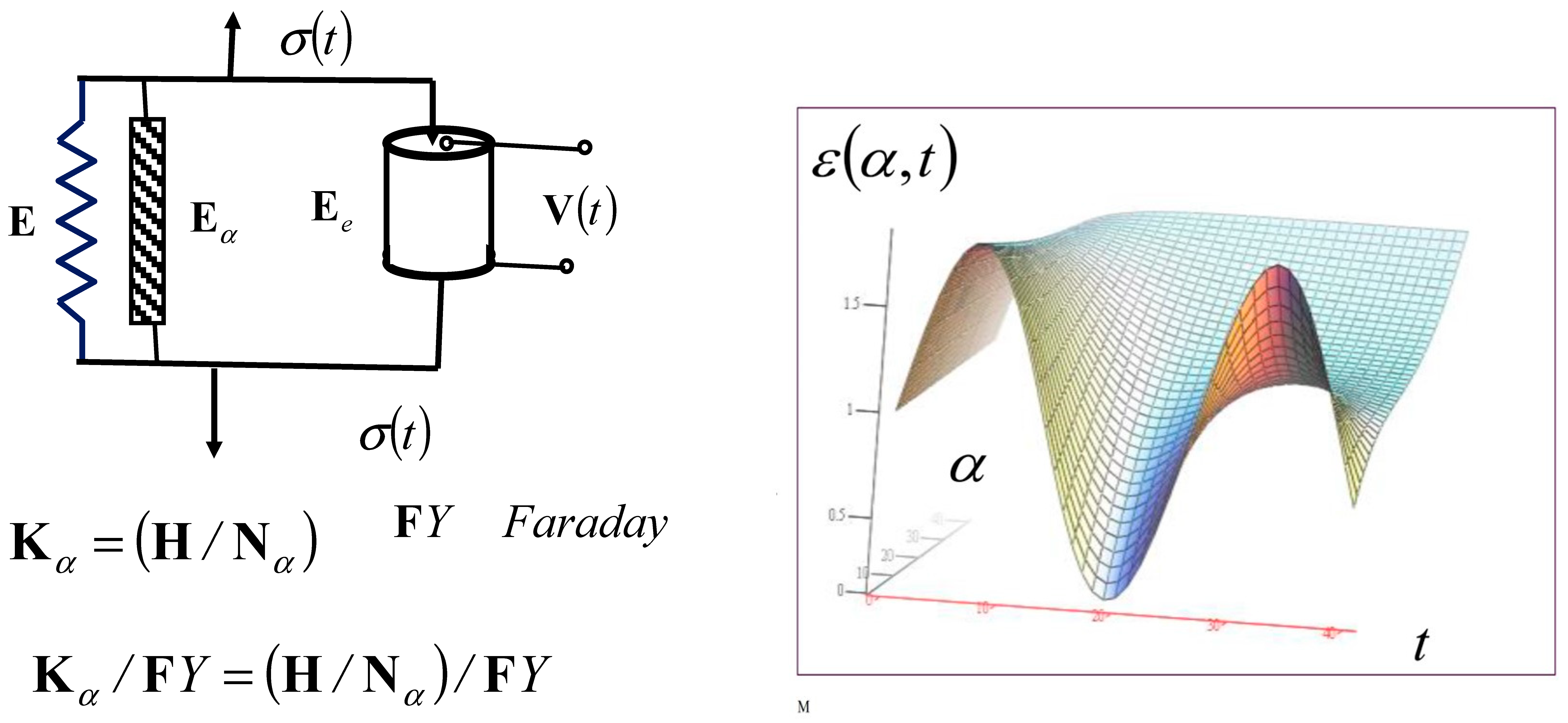
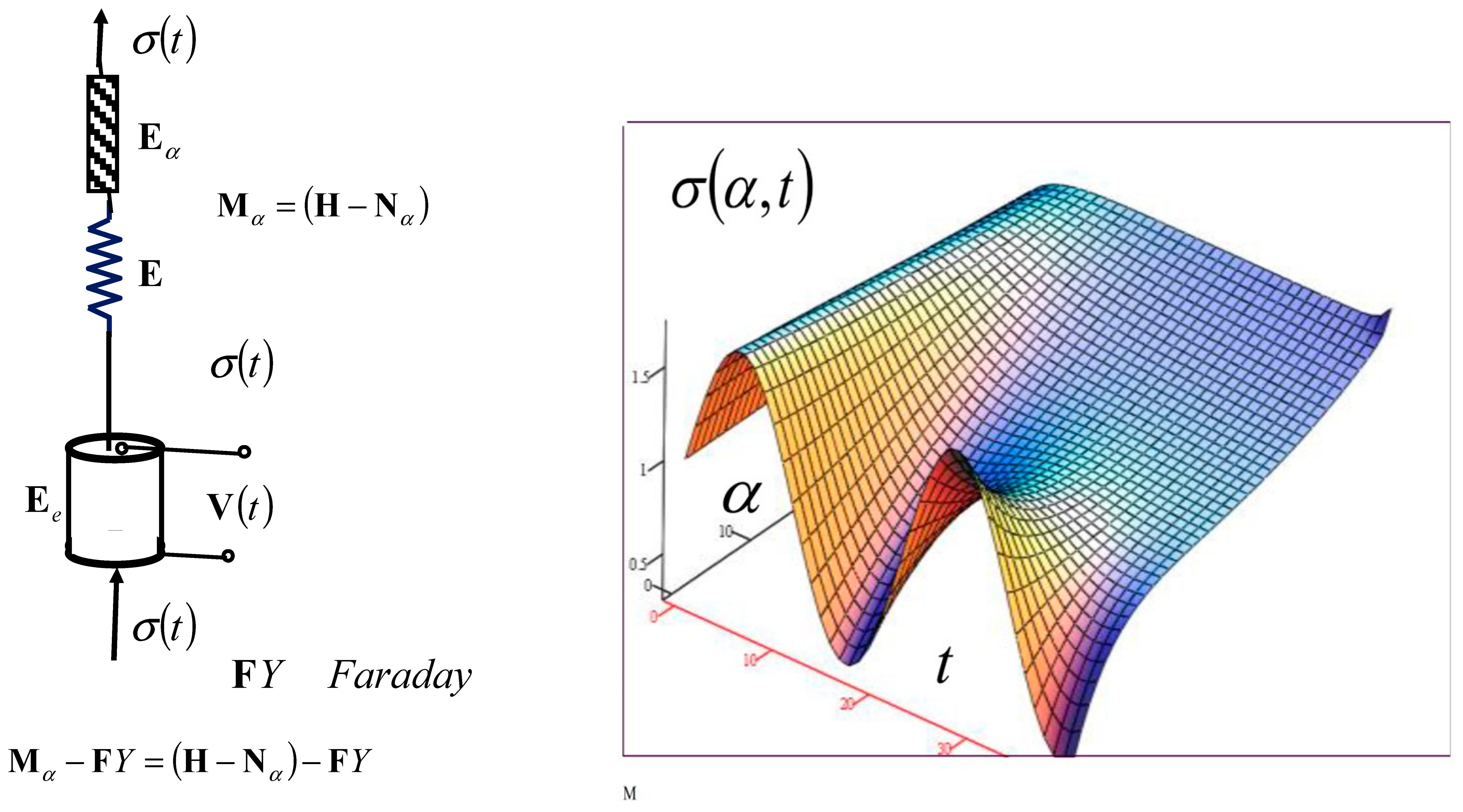
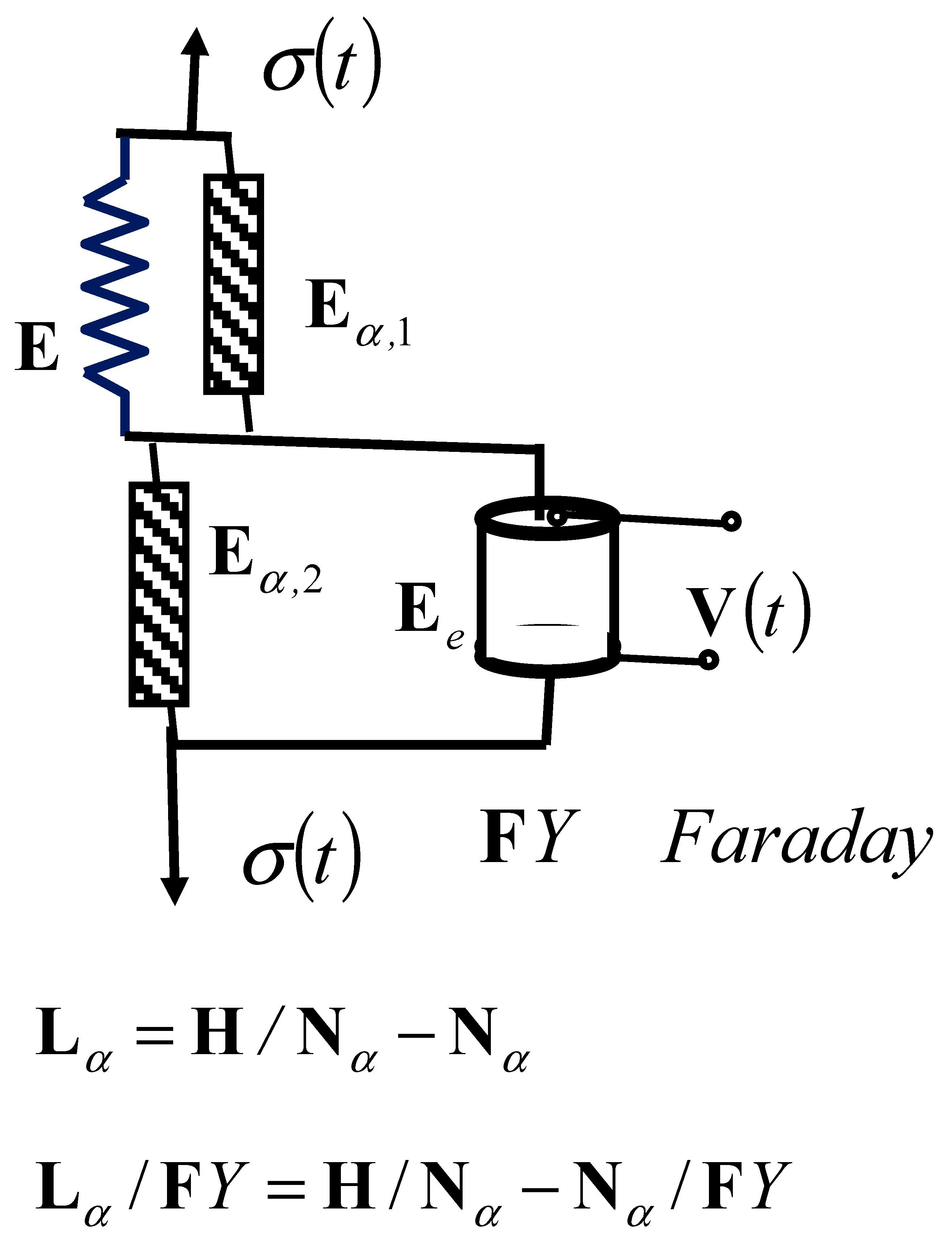
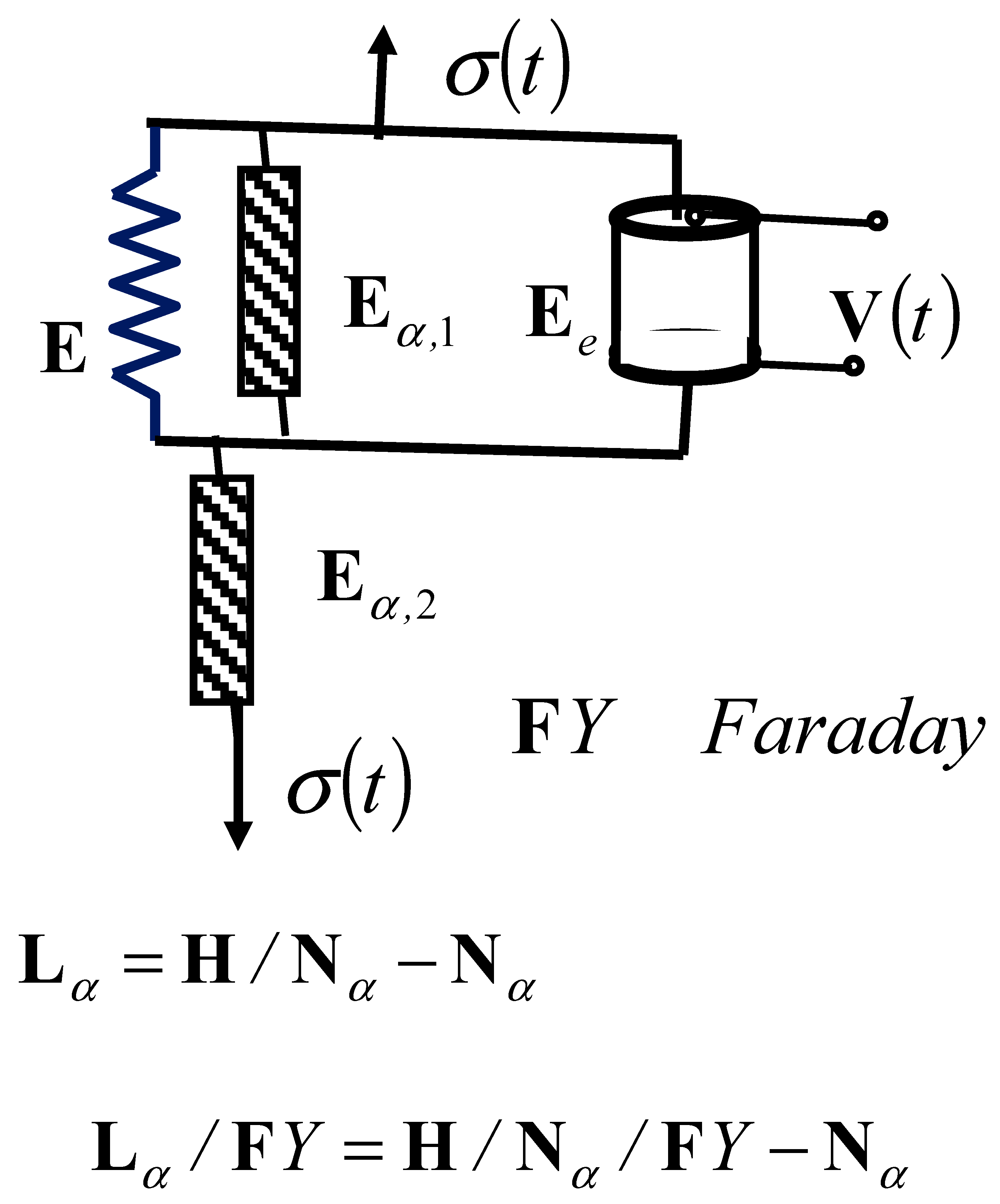
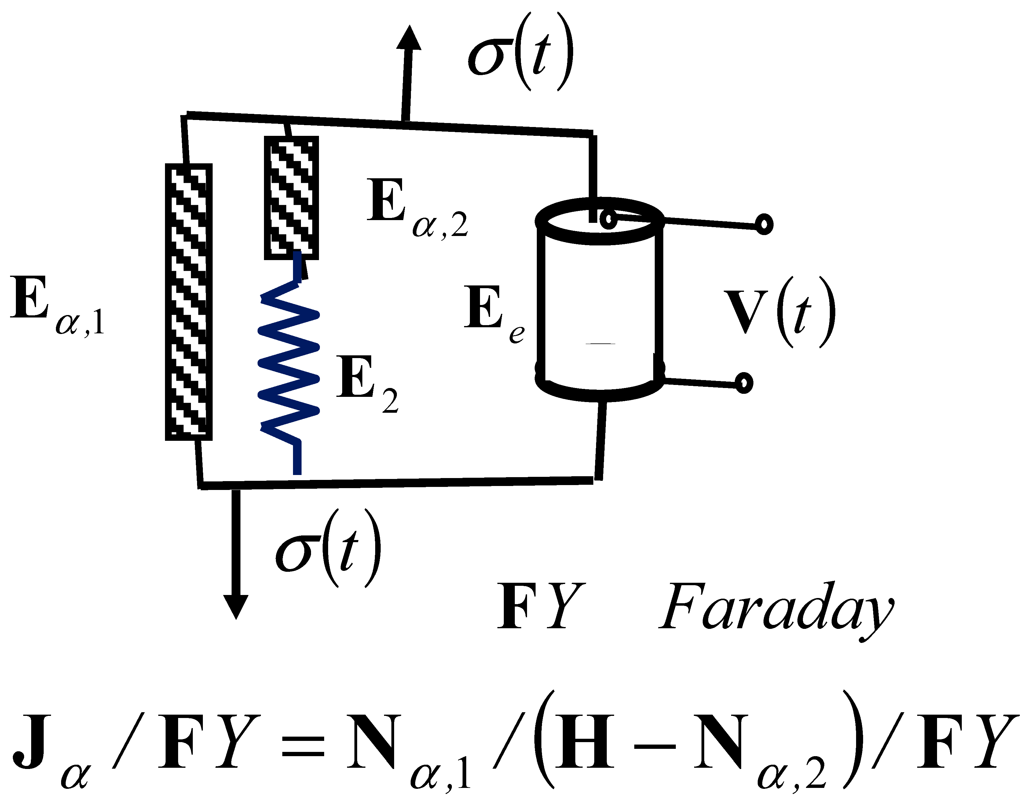
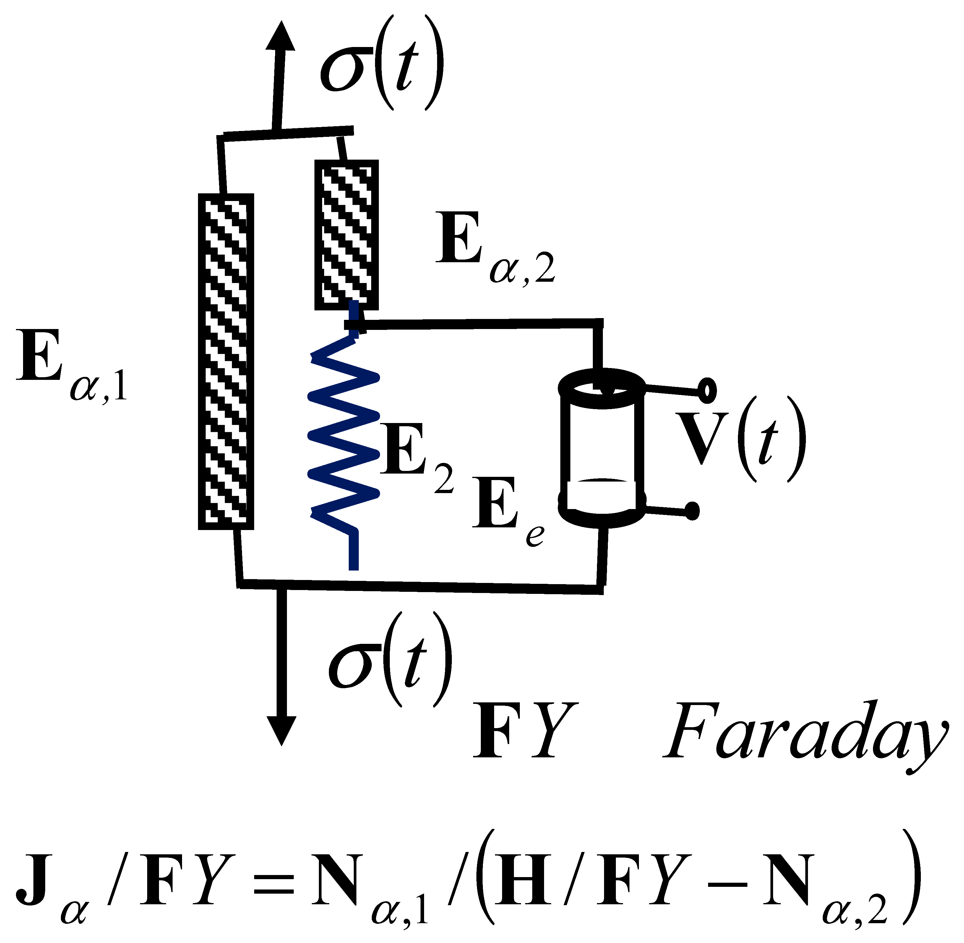
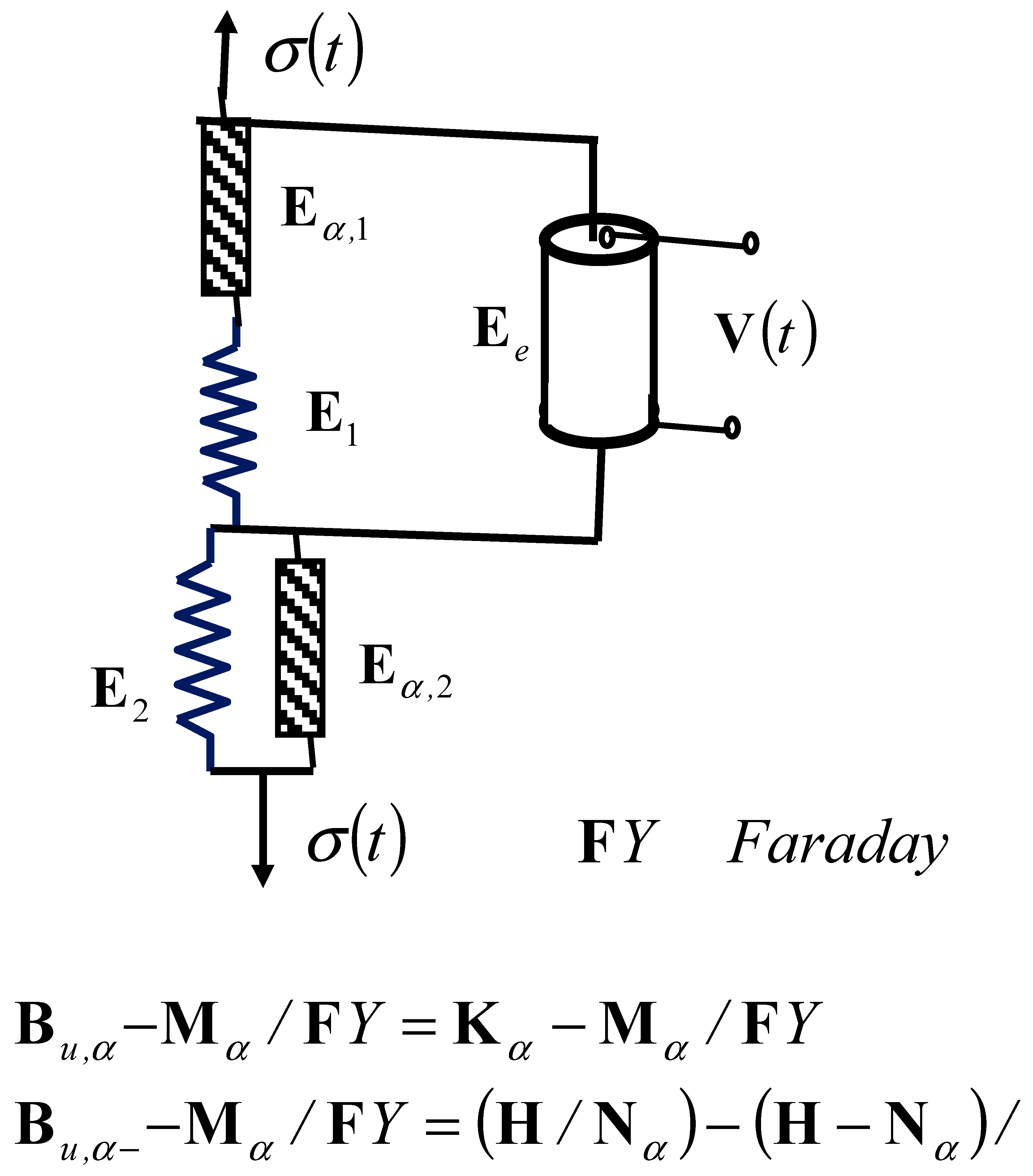
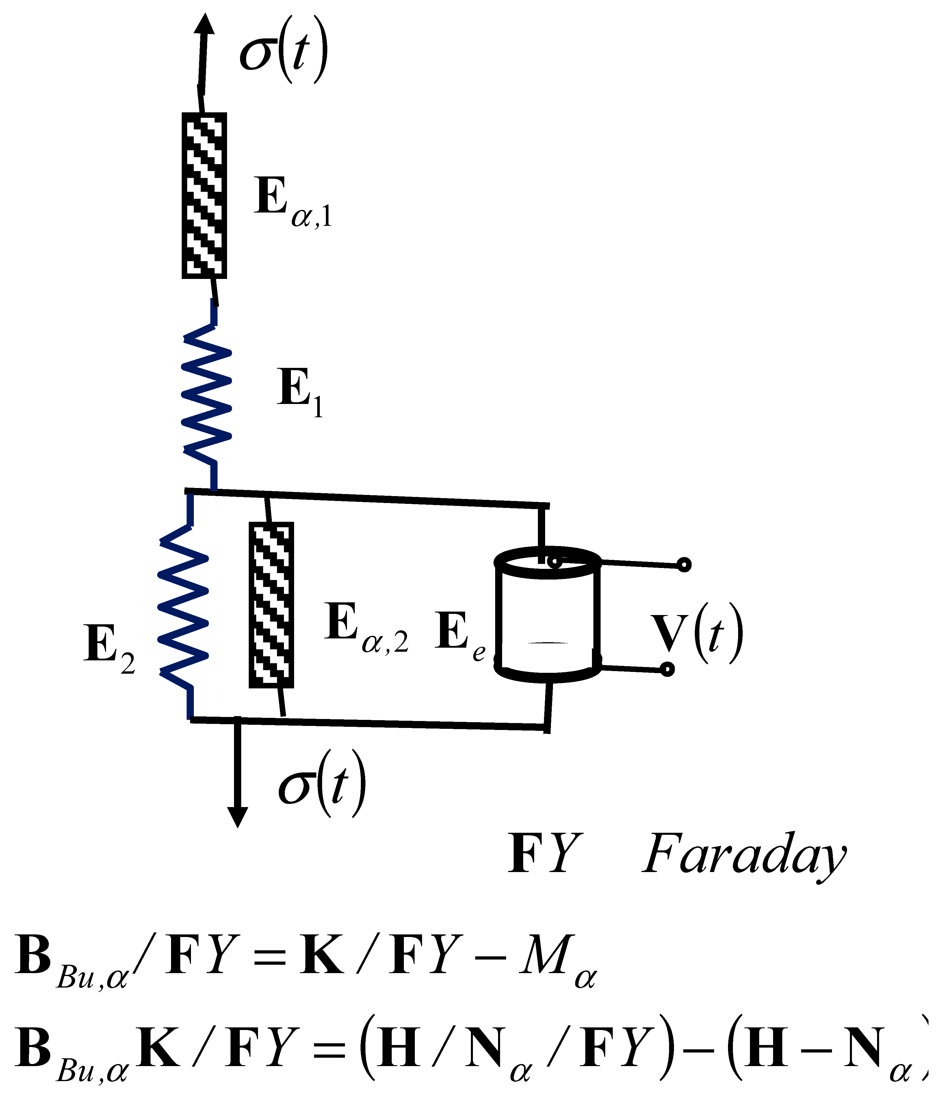
Disclaimer/Publisher’s Note: The statements, opinions and data contained in all publications are solely those of the individual author(s) and contributor(s) and not of MDPI and/or the editor(s). MDPI and/or the editor(s) disclaim responsibility for any injury to people or property resulting from any ideas, methods, instructions or products referred to in the content. |
© 2025 by the author. Licensee MDPI, Basel, Switzerland. This article is an open access article distributed under the terms and conditions of the Creative Commons Attribution (CC BY) license (https://creativecommons.org/licenses/by/4.0/).