Integrating Multifractal Features into Machine Learning for Improved Prediction

Abstract

This study investigates the multifractal characteristics of the tanker freight market from 1998 to 2024. Using multifractal detrended fluctuation analysis (MF-DFA) and multifractal detrending moving average (MF-DMA), we analyze temporal correlations and volatility, revealing subtle differences in multifractal features before and after 2010. We further examine the influence of key external factors—including economic disturbances (the 2008 financial crisis), technological innovations (the 2014 Shale Oil Revolution), supply chain disruptions (the COVID-19 pandemic), and geopolitical uncertainties (the Russia–Ukraine conflict)—on market complexity. Building on this, a predictive framework is introduced, leveraging the Baltic Dirty Tanker Index (BDTI) to forecast Brent oil prices. By integrating multifractal analysis with machine learning models (e.g., XGBoost, LightGBM, and CatBoost), our framework fully exploits the predictability from the freight index to oil prices across the above four major global events. The results demonstrate the potential of combining multifractal analysis with advanced machine learning models to improve forecasting accuracy and provide actionable insights during periods of heightened market volatility. On average, the coefficient of determination (R²) increases by approximately 62.65% to 182.54% for training and 55.20% to 167.62% for testing, while the mean squared error (MSE) reduces by 60.83% to 92.71%. This highlights the effectiveness of multifractal analysis in enhancing model performance, especially in more complex market conditions post-2010.

1. Introduction

The global tanker freight market plays a crucial role in the shipping industry and has long been a focus for both academicians and industry practitioners [1,2,3]. This market exhibits complex behaviors driven by geopolitical events [4,5,6], economic conditions [7], technological innovations, and environmental policies [8]. Its inherent volatility and multi-scale temporal correlations further complicate the study of market dynamics [9,10]. Understanding these trends is essential for stakeholders seeking to navigate market shifts and leverage technological advancements [11,12,13,14,15,16,17,18].

Despite growing interest in this field, several key gaps remain. There is a need for a deeper understanding of how multifractal dynamics in the tanker freight market interact with external influences, such as geopolitical tensions, economic cycles, and environmental policies [4,9]. Additionally, more interdisciplinary research is required, integrating insights from complexity economics, financial engineering, and operations research to develop more advanced methodologies for analyzing and managing risks in this evolving market [19,20,21].

Complexity economics provides an interdisciplinary framework that integrates economics, information science, physics, and operations research [22,23,24]. It recognizes agent heterogeneity, imperfect information, and dynamic system behavior, offering valuable insights into energy and tanker freight markets [4,12,25,26,27,28]. Fractals, characterized by self-similarity and fragmented geometric structures, have become an effective tool in complexity economics [29,30]. Early methodologies, such as Hurst’s rescaled range analysis, struggled to assess long-range dependencies in nonstationary series [31]. To address this, Castro et al. introduced a novel approach for multi-affine fractal exponents and correlation coefficients [32], while Peng et al. developed a detrended fluctuation analysis (DFA) to quantify long-term correlations [33]. However, DFA was limited in capturing multi-scale and fractal structures, necessitating the development of multifractal detrended fluctuation analysis (MF-DFA) by Kantelhardt et al. [34], which has since become a standard tool for multifractal characterization [35,36]. In parallel, the detrending moving average (DMA) technique emerged as an effective method for analyzing long memory in nonstationary time series [37,38,39]. By refining the moving average function, DMA excels in detecting scaling properties [40], with MF-DMA extending its application to higher dimensions. This method helps distinguish true multifractality—arising from nonlinear correlations—from spurious effects caused by fat-tailed probability distributions [41,42]. Kwapien et al. further confirmed that true multifractality in time series originates from temporal correlations using both analytical and numerical evidence [43].

To provide a clearer understanding of the methods used in this study, we present a comparative chart outlining the key differences between the MF-DFA, MF-DMA, and conventional methods. As shown in

Table 1. Comparison of MF-DFA, MF-DMA, and conventional methods.

Method	Core Principle	Advantages	Limitations	Applicability
MF-DFA	Detrends time series and analyzes multifractal behavior	Captures nonlinear, scale-dependent fluctuations	Can be technically complex	Well-suited for non-stationary data
MF-DMA	Uses moving averages for detrending and multifractal analysis	Simpler implementation than MF-DFA	May be less robust under certain conditions	Good for smoother data trends
Conventional Methods	Often rely on linear assumptions or static models	Easier to implement and interpret	Fail to capture dynamic, multifractal behavior	Limited when dealing with high complexity

, this comparison highlights the core principles, advantages, limitations, and applicability of each method in analyzing multifractal behavior in the tanker freight market.

Research on tanker freight rate volatility is a key area in maritime economics, influencing the broader global economy. These studies explore the interplay of factors such as crude oil prices, charter rates, fleet size, and policy changes [13,14,15,16,17,18,19,44]. Multifractal analysis has gained traction in this field for its ability to capture asymmetric market risks, revealing varying responses to upward and downward trends and identifying distinct scaling behaviors [45]. Unlike traditional methods, multifractality recognizes that freight rates exhibit a spectrum of fractal characteristics rather than a single fluctuation pattern [46,47,48,49]. It accounts for both small and large market movements, offering a nuanced perspective on data correlations, particularly during turbulent periods, such as the 2008 financial crisis and the COVID-19 pandemic [4,12,46]. This study aims to analyze the market’s evolving complexity, providing insights into its long-term dynamics and informing strategies to mitigate the impact of unpredictable market changes and crises. This study tries to comprehend the intricate, multifaceted nature of the market to provide a comprehensive understanding of the market’s complexity and its evolution over time and design strategies that buffer the fallout from unpredictable market shifts or crises.

The research is driven by the following key questions: (a) How has the multifractal nature of the tanker freight market evolved across two distinct periods—1998–2010 and 2010–2024—and what insights does this evolution provide regarding market behavior and systemic risks? (b) What role do temporal correlations and inherent volatility play in shaping the complex structure of the market, and how do these factors contribute to the observed multifractal dynamics? (c) How do external factors shape the complexity and multifractal characteristics of the tanker freight market, particularly through financial crises, supply chain disruptions, regulatory interventions, technological advancements in energy efficiency, and carbon emission policies? (d) Can tanker freight rates, specifically the Baltic Dirty Tanker Index (BDTI, a vital benchmark that assesses the cost of shipping dirty petroleum products, including crude oil, on selected routes within the Baltic region), be used to predict Brent oil prices during periods of heightened market complexity, and how do multifractal features enhance the predictive power of such models?

This study investigates the complexity and multifractal characteristics of the Baltic Clean and Dirty Tankers markets from 1998 to 2023. Using MF-DFA, we analyze clean and dirty tanker freight rates, specifically the TC2 and TD7 routes, from 28 January 1998, to 12 January 2024. To examine market patterns following major fluctuations, we compare Period I (1998–2010) and Period II (2010–2024). Additionally, to better understand the multifractality of Baltic Dirty Tanker Index (BCTI, a widely recognized benchmark that tracks freight rates for large capesize vessels and reflects global shipping market conditions), we employ MF-DMA to quantify three key components: linear correlation, nonlinear correlation, and fat-tailed probability distribution.

Building on this foundational analysis, we further extend the scope of our research to explore the predictive potential of freight rates in forecasting Brent oil prices, particularly during periods of heightened market volatility and complexity. Traditionally, most studies have focused on forecasting freight rates based on oil price movements, reflecting the conventional economic logic that oil prices drive downstream costs, including shipping. Numerous studies support this view, emphasizing the dominant role of oil prices in shaping the freight market. For instance, Alizadeh and Nomikos (2004) examined the cost-of-carry relationship between oil futures and freight markets, but found no significant link that would allow freight rates to predict oil price movements [50]. Similarly, Gavriilidis et al. (2018) utilized GARCH-X models and demonstrated that oil price shocks, particularly demand and precautionary demand shocks, significantly affect freight rate volatility, yet their findings did not establish freight rates as an effective predictor of oil price fluctuations [14]. Shi et al. (2022) further explored the dynamic dependence between these markets through a copula-MIDAS-X model, concluding that oil price non-supply shocks played a crucial role in shaping freight rate behavior, while freight rates themselves lacked substantial feedback effects on oil prices [51]. Furthermore, Siddiqui and Basu (2020), by decomposing cyclical components of oil prices and freight rates, reaffirmed the prevailing view that oil prices generally lead freight rate movements over medium- to long-term cycles, underscoring the asymmetric influence of oil prices over the shipping sector [18]. However, freight rates, due to their responsiveness to supply–demand dynamics, vessel utilization rates, and macroeconomic shifts, may serve as valuable leading indicators for oil prices. This study, therefore, adopts an innovative perspective by investigating whether BDTI can predict Brent oil prices and how multifractal features contribute to the accuracy of such predictions.

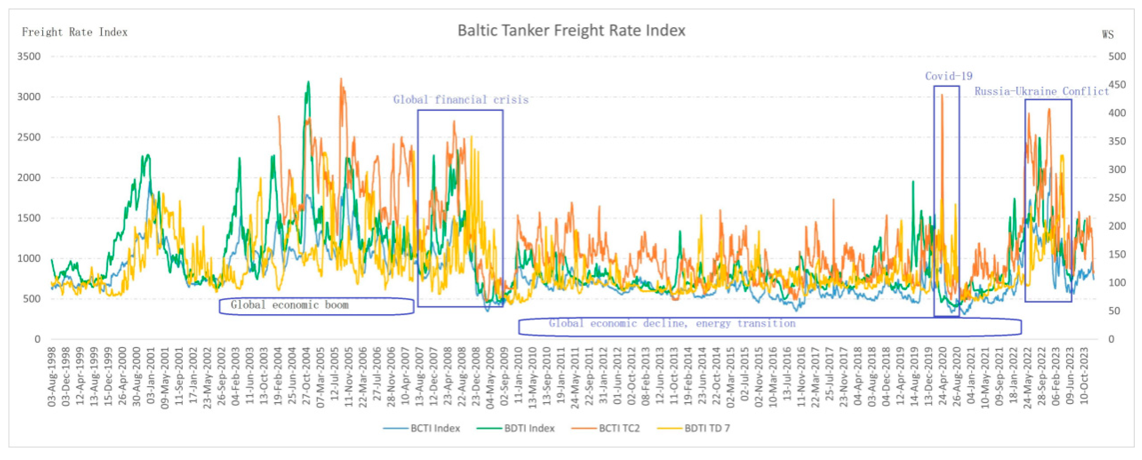
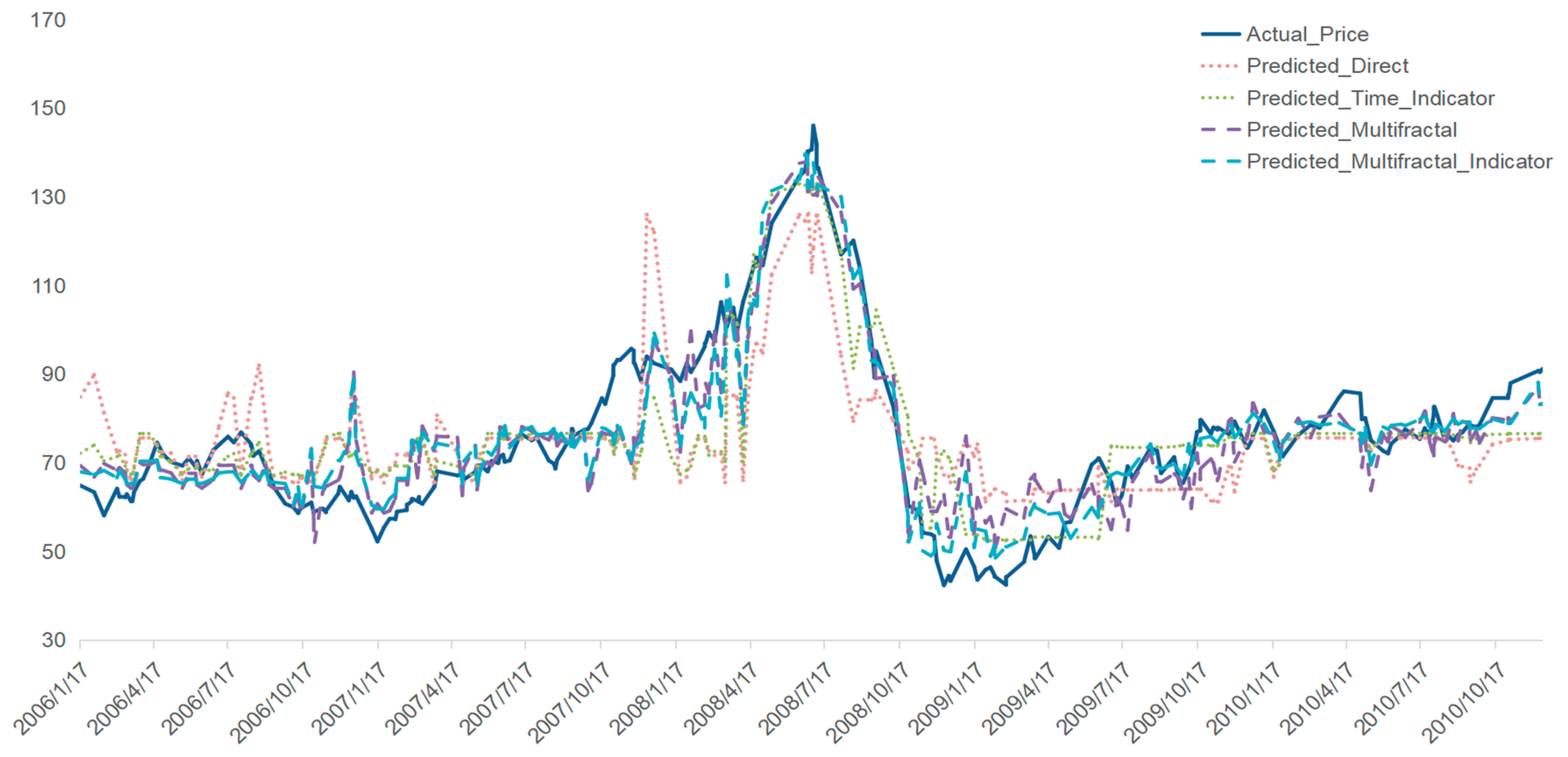
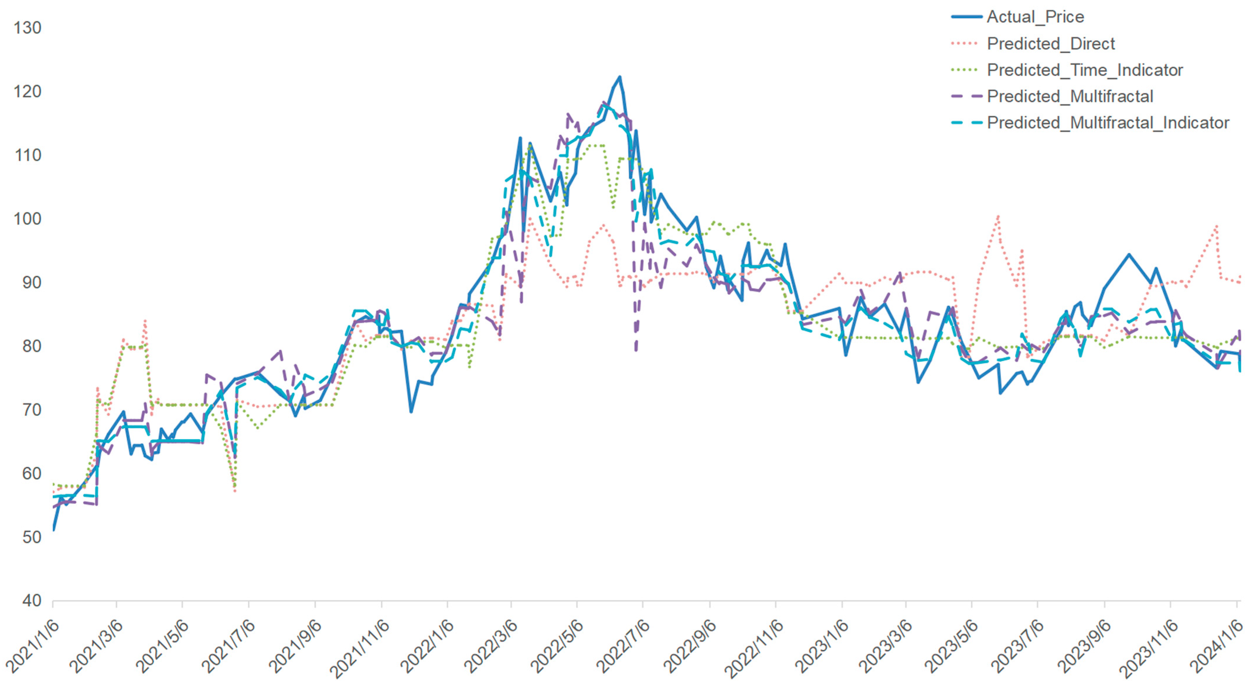
To address this question, we examine four distinct periods characterized by major global events that significantly influenced market dynamics: (1) 2006–2010: marked by the 2008 global financial crisis, which caused widespread disruptions in financial and commodity markets; (2) 2013–2016: defined by the 2014 Shale Oil Revolution, which reshaped global energy supply dynamics; (3) 2019–2021: dominated by the COVID-19 pandemic, leading to unprecedented supply chain disruptions; and (4) 2021–2024: influenced by the Russia–Ukraine conflict, introducing severe geopolitical uncertainties and energy market volatility.

For each period, we develop predictive models using BDTI data as the primary feature, incorporating multifractal characteristics extracted via MF-DFA, such as the Hurst exponent and multifractal spectrum. To capture market dynamics during global events, these models are further enhanced with crisis period indicators. To improve prediction robustness, we employ stacking regression, integrating XGBoost, LightGBM, and CatBoost as base learners [52,53,54]. XGBoost, known for its scalability and efficiency, delivers state-of-the-art performance across various machine learning tasks [55]. Ridge Regression serves as the meta-learner, refining the final predictions. By structuring these powerful algorithms systematically, we enhance the accuracy and stability of our models, ensuring more reliable and insightful outcomes [56].

The major contribution of this study is summarized as follows. The methodology evaluates the individual and combined effects of multifractal features and crisis indicators on predictive accuracy. This comprehensive framework not only assesses the predictive capacity of freight rates for oil prices but also provides deeper insights into how economic and geopolitical crises influence market dynamics. In addition, this study offers valuable insights for investors, energy companies, and policymakers. For investors, the enhanced predictive models enable better risk management and informed decision-making, especially during periods of market volatility. Companies can optimize trading strategies and hedge against price fluctuations by leveraging the predictive power of the Baltic Dirty Tanker Index (BDTI) and multifractal features. Policymakers can develop more effective regulations to promote market stability and mitigate systemic risks by understanding the multifractal nature of tanker freight markets. Overall, this research provides a robust framework for stakeholders to explore market complexities and enhance resilience in the face of global uncertainties. The integration of multifractal analysis with predictive modeling demonstrates the potential for advanced analytics to effectively navigate the complexities of modern financial markets.

The paper structure is as follows: Section 2 introduces the MF-DFA and MF-DMA methods, and Section 3 describes the Baltic Clean and Dirty Tanker Indexes and the data used in the analysis. Section 4 presents the empirical results, including the multifractal characteristics of freight rate returns, the impact of structural breaks across different periods, and the predictive performance of the proposed framework under varying market conditions. Section 5 discusses the implications of the findings for market participants, including investors, energy companies, and policymakers, and suggests potential directions for future research. Section 6 concludes the study with key insights and future research directions.

2. Methods

2.1. The Multifractal Detrended Fluctuation Analysis Method

The following introduction of the MF-DFA method is based on the work by Kantelhardt et al. (2002) [34].

Here are the general steps of the MF-DFA method on the series $x\left(i\right)$, where $i=1,2,\dots ,N$ and $N$ is the length of the series. $\overline{x}$ stands for the average value of series $x\left(i\right)$.

Assuming that $x\left(i\right)$ are increments of a random walk process around the mean $\overline{x}$, the “trajectory” or “profile”, by the signal integration, could be expressed as

$$\mathrm{y}\left(\mathrm{i}\right)={\sum }_{\mathrm{k}=1}^{\mathrm{i}}\left[\mathrm{x}\right(\mathrm{k})-\overline{\mathrm{x}}], \mathrm{i}=1,2,\dots ,\mathrm{N}$$

(1)

Segment Division: We divide the integrated series into $N_s=\mathrm{i}\mathrm{n}\mathrm{t}\left(N/s\right)$, non-overlapping segments of equal length $s$. Generally, the length $N$ of the series is not a multiple of the considered time scale $s$, and a short part may remain at the end of the profile $y\left(i\right)$. Not to disregard this remaining part, this procedure is repeated in reverse, starting from the end. So, $2N_s$ segments are obtained.

Detrending: The local trend for each of the $2N_s$ segments could be calculated by a least-square fit of the series. Then, the variance is determined by

$${\mathrm{F}}^2(\mathrm{s},\mathrm{v})=1/\mathrm{s}\times {\sum }_{\mathrm{i}=1}^{\mathrm{s}}\left\{\mathrm{y}\right[(\mathrm{v}-1)\mathrm{s}+\mathrm{i}]-{\mathrm{y}}_{\mathrm{v}}\left(\mathrm{i}\right){\}}^2$$

(2)

For each segment $v$, $v=1,\dots ,Ns$ and

$${\mathrm{F}}^2(\mathrm{s},\mathrm{v})=1/\mathrm{s}\times {\sum }_{\mathrm{i}=1}^{\mathrm{s}}\left\{\mathrm{y}\right[(\mathrm{N}-(\mathrm{v}-{\mathrm{N}}_{\mathrm{s}})\mathrm{s}+\mathrm{i}]-{\mathrm{y}}_{\mathrm{v}}\left(\mathrm{i}\right){\}}^2$$

(3)

for $v=\mathrm{N}\mathrm{s}+1,\dots ,2\mathrm{N}\mathrm{s}$. Here, $y_v\left(i\right)$ is the fitting line in segment $v$.

Fluctuation Function ${\mathrm{F}}_{\mathrm{q}}\left(\mathrm{s}\right)$: All segments are averaged to obtain the $q$-th order fluctuation function by

$${\mathrm{F}}_{\mathrm{q}}\left(\mathrm{s}\right)=\left\{1/\mathrm{s}\times {\mathrm{N}}_{\mathrm{s}}\right.{\left.{\sum }_{\mathrm{v}=1}^{2{\mathrm{N}}_{\mathrm{s}}}\left[{\mathrm{F}}^2(\mathrm{s},\mathrm{v}{)}^{\mathrm{q}/2}\right]\right\}}^{1/\mathrm{q}}$$

(4)

where the index variable $q$ can generally take any real value except zero.

Scaling Exponent $h_q$: Repeating the above steps for several time scales $\mathrm{s}$, $F_q\left(s\right)$ will increase as $s$ increases. The scaling behavior of the fluctuation functions could be analyzed using log–log plots $F_q\left(s\right)$ versus $s$ for each value of $q$. A power-law between $F_q\left(s\right)$ and $s$ exists, as shown in Equation (5), when the series $x\left(i\right)$ exhibits a long-range power-law correlation.

$${\mathrm{F}}_{\mathrm{q}}\left(\mathrm{s}\right)\approx {\mathrm{s}}^{{\mathrm{h}}_{\mathrm{q}}}$$

(5)

However, because of the diverging exponent, the averaging procedure of Equation (4) could not be applied directly to calculate the value $h_0$, which corresponds to the limit $h_q$ as $q\to 0$. Instead, we must employ a logarithmic averaging procedure using Equation (6).

$${\mathrm{F}}_0\left(\mathrm{s}\right)=\exp \left\{1/4\times {\mathrm{N}}_{\mathrm{s}}\right.\left.{\sum }_{\mathrm{v}=1}^{2{\mathrm{N}}_{\mathrm{s}}}\ln \left[{\mathrm{F}}^2(\mathrm{s},\mathrm{v})\right]\right\}\approx {\mathrm{s}}^{{\mathrm{h}}_0}$$

(6)

The exponent $h_q$ generally depends on $q$. For the stationary series, $h_2$ is the well-defined Hurst exponent $H$. Therefore, $h_q$ is called the generalized Hurst exponent. In a special case, when $h_q$ is independent of $q$, it is defined as a monofractal series. The distinct scaling patterns exhibited by small and large fluctuations have a substantial impact on the relationship between the $q$-th-order Hurst exponent $h_q$ and the scaling parameter $q$. In the case of positive $q$, segments $v$ characterized by a significant deviation from the expected trend, i.e., those with large variances, will exert a dominant influence on the average $q$-order Hurst exponent $F_q\left(s\right)$. Consequently, a positive $q$ captures the scaling behavior of the segments $v$ with notable fluctuations, which typically correspond to smaller scaling exponents in multifractal time series. Conversely, for negative $q$ values, the segments $v$ with smaller variances take precedence in determining the average $q$-order Hurst exponent $F_q\left(s\right)$. Hence, a negative $q$ describes the scaling behavior of segments $v$ with minor fluctuations, which generally exhibit larger scaling exponents in multifractal time series. This intricate interplay between $q$, the scaling behavior of different segments $v$, and the corresponding fluctuations provides valuable insights into the multifractal nature of the time series, shedding light on how various levels of variance impact the overall scaling exponents.

Let us take a simple example using a small synthetic time series of length $\mathrm{N}=100$:

Step 1: Calculate the profile by subtracting the mean and performing the cumulative sum:

$$\mathrm{y}\left(\mathrm{i}\right)=\sum _{\mathrm{k}=1}^{\mathrm{i}}\left[\mathrm{x}\right(\mathrm{k})-\overline{\mathrm{x}}], \mathrm{i}=1,2,\dots ,100$$

Step 2: Divide the profile into segments of size $s=10$, resulting in 10 segments.

Step 3: Perform local detrending for each segment by fitting a linear polynomial (least-squares fit) and subtracting the fit from the data.

Step 4: Calculate the fluctuation function for different values of q, e.g., q = 1, 2, −1.

Step 5: Analyze the scaling of $F_q\left(s\right)$ with $s$ and estimate the generalized Hurst exponent $h_q$.

This procedure allows you to assess the multifractal characteristics of the time series, as the scaling behavior reveals information about the correlation and variance of the series across different scales.

The multifractal spectrum $f\left(\alpha \right)$ is another tool to characterize multifractality in a series. $f\left(\alpha \right)$ can be obtained by Equation (7):

$$\mathsf{\tau }\left(\mathrm{q}\right)=\mathrm{q}{\mathrm{h}}_{\mathrm{q}}-1$$

(7)

and then the Legendre transform

$$\mathsf{\alpha }=\mathrm{d}\mathsf{\tau }/\mathrm{dq}$$

(8)

$$\mathrm{f}\left(\mathrm{q}\right)=\mathrm{q}\mathsf{\alpha }-\mathsf{\tau }\left(\mathrm{q}\right)$$

(9)

where $\alpha$ is the Holder exponent value, which indicates the strength of singularity. When $f\left(\alpha \right)$ is broader, it indicates a stronger multifractality or complexity.

The width of the spectrum could be

$$\mathsf{\Delta }\mathsf{\alpha }={\mathsf{\alpha }}_{\max }-{\mathsf{\alpha }}_{\min }$$

(10)

where ${\alpha }_{max}$ and ${\alpha }_{min}$ indicate the maximum and minimum values, respectively.

We name MF-DFA1, MF-DFA2, and MF-DFA3 separately with polynomial order $m=1,2,3$. Here, we apply MF-DFA1 and MF-DFA2 to investigate the BCTI, BDTI, and specific routes of TC2 and TD7.

To realize this process, we use Matlab R2024b and Jupyter Notebook (https://jupyter.org/).

2.2. The Multifractal Detrending Moving Average Method

The following brief introduction of the MF-DMA method is based on the works of Gu and Zhou (2010) [41].

Assuming time series $x\left(t\right)$, $t=1,2,\cdots ,N$, and $N$ is the length of the series. We construct a new series:

$$\mathrm{y}\left(\mathrm{t}\right)={\sum }_{\mathrm{i}=1}^{\mathrm{t}}\mathrm{x}\left(\mathrm{i}\right),\mathrm{t}=1,2,\cdots ,\mathrm{N}$$

(11)

In the next step, $\tilde{y}\left(t\right)$ indicates the moving average function. To calculate the sequence of cumulative totals, we slide a window of fixed size across the sequence:

$$\stackrel{\mathrm{~}}{\mathrm{y}}\left(\mathrm{t}\right)=1/\mathrm{n}\times {\sum }_{\mathrm{k}=-⌊\left(\mathrm{n}-1\right)\mathsf{\theta }⌋}^{⌈\left(\mathrm{n}-1\right)\left(1-\mathsf{\theta }\right)⌉}\mathrm{y}(\mathrm{t}-\mathrm{k})$$

(12)

where $n$ is the size of window, $⌊x⌋$ is the largest integer but not greater than $x$, $⌈x⌉$ is the smallest integer but not smaller than $x$, and $\theta$ is the position parameter, varying from 0 to 1. Here $\tilde{y}\left(t\right)$ is calculated over $⌈\left(n-1\right)\left(1-\theta \right)⌉$ data points from the preceding period but $⌊\left(n-1\right)\theta ⌋$ data points from the subsequent period. We must notice three special cases with different $\theta$ values. The backward-moving average, where $\theta =0$ and $\tilde{y}\left(t\right)$, is calculated using all the past data points. $\theta =0.5\mathrm{r}$ efers to the centered moving average, where $\tilde{y}\left(t\right)$ is calculated over half past and half future data points. $\theta =1$ represents the forward-moving average, where $\tilde{y}\left(t\right)$ is based on the trend of future data points. In this context, we utilize the selected case $\theta =0$, as it has demonstrated superior performance compared to the other two alternatives, based on the evidence presented in references [37,41,43].

Subsequently, we eliminate the moving average component $\tilde{y}\left(i\right)$ from the series $y\left(i\right)$ to eliminate any underlying trend, resulting in a residual sequence $\epsilon \left(i\right)$:

$$\mathsf{\epsilon }\left(\mathrm{i}\right)=\mathrm{y}\left(\mathrm{i}\right)-\stackrel{\mathrm{~}}{\mathrm{y}}\left(\mathrm{i}\right)$$

(13)

where $\mathrm{n}-⌊\left(\mathrm{n}-1\right)\mathsf{\theta }⌋\le \mathrm{i}\le \mathrm{N}-⌊(\mathrm{n}-1)\mathsf{\theta }⌋$.

Then, the residual series $\epsilon \left(i\right)$ is divided into $N_n$ ($N_n=⌊N/n-1⌋$) non-overlapping segments, each of equal length $n$. These segments can be represented as ${\epsilon }_v\left(i\right)=\epsilon (l+i)$ for $1\le i\le n$, where $l=(v-1)n$. We can obtain the root-mean-square function $F_v\left(n\right)$ using Equation (14).

$${\mathrm{F}}_{\mathrm{v}}^2\left(\mathrm{n}\right)=1/\mathrm{n}\times {\sum }_{\mathrm{i}=1}^{\mathrm{n}}{\mathsf{\epsilon }}_{\mathrm{v}}^2\left(\mathrm{i}\right),$$

(14)

Additionally, the $q$-th-order overall fluctuation function $F_q\left(n\right)$ is expressed as

$${\mathrm{F}}_{\mathrm{q}}\left(\mathrm{n}\right)={\left\{1/{\mathrm{N}}_{\mathrm{n}}\times {\sum }_{\mathrm{v}=1}^{{\mathrm{N}}_{\mathrm{n}}}{\mathrm{F}}_{\mathrm{v}}^{\mathrm{q}}\left(\mathrm{n}\right)\right\}}^{1/\mathrm{q}}, \mathrm{q}\ne 0$$

(15)

$$\ln \left[{\mathrm{F}}_0\left(\mathrm{n}\right)\right]=1/{\mathrm{N}}_{\mathrm{n}}\times {\sum }_{\mathrm{v}=1}^{{\mathrm{N}}_{\mathrm{n}}}\ln \left[{\mathrm{F}}_{\mathrm{v}}\left(\mathrm{n}\right)\right], \mathrm{q}=0$$

(16)

When the values of $n$ varies, we can get the power-law relation between $F_q\left(n\right)$ and $n$ in Equation (17):

$${\mathrm{F}}_{\mathrm{q}}\left(\mathrm{n}\right)~{\mathrm{n}}^{\mathrm{h}\left(\mathrm{q}\right)}$$

(17)

Finally, the multifractal scaling exponent $\tau \left(q\right)$ and multifractal spectrum $f\left(q\right)$ could be defined similarly to that of the above MF-DFA.

2.3. The Effective Multifractality

According to the references [57,58], the total multifractal spectrum could be intricately divided into three parts: the nonlinear (NL) and linear correlation (LM), and the probability density function (PDF). This decomposition is captured by Equation (18):

$$\mathsf{\Delta }\mathsf{\alpha }=\mathsf{\Delta }{\mathsf{\alpha }}_{\mathrm{NL}}+\mathsf{\Delta }{\mathsf{\alpha }}_{\mathrm{LM}}+\mathsf{\Delta }{\mathsf{\alpha }}_{\mathrm{PDF}}$$

(18)

It is important to emphasize that both the linear correlation component $\mathsf{\Delta }{\alpha }_{LM}$ and the nonlinear correlation component $\mathsf{\Delta }{\alpha }_{NL}$ represent temporal correlations [2,5]. Specifically, the linear correlation component is attributed to finite-size effects [52,58]. Furthermore, it is noteworthy that $\mathsf{\Delta }{\alpha }_{LM}$, indicating the linear correlation component, can be computed using semi-analytical formulas of an explicit form, offering a comprehensive quantitative characterization of this phenomenon [39]. A type of computational deviation stemming from the sample number constraints is defined as the finite-size effect in reference [26]. In essence, smaller time series sizes lead to greater computation deviations. To mitigate the impact of sample size limitations, especially for small sample sizes <10,000, it is necessary to calculate and exclude the linear correlation component from the true multifractality. Consequently, the true multifractality, denoted as $\mathsf{\Delta }{\alpha }_{eff}$, which encompasses the nonlinearity component $\Delta {\alpha }_{NL}$ and the PDF component $\mathsf{\Delta }{\alpha }_{PDF}$, is determined [40,57,59].

To depict the spectrum of multifractality, it is important to conduct an analysis that involves both the elimination of the linear correlation component stemming from the sample size limitations (sample size < 10,000 points) and the decomposition of the remaining two effective parts [57,59,60]. This quantitative analysis can be achieved through the creation of two new series: the shuffled and the surrogate time series. The shuffled time series is generated through the shuffled original series. During this process, the temporal correlations are disrupted, while the probability distribution remains unaltered [43,59].

The creation of surrogate data is accomplished through a two-stage procedure. Initially, the process ensures that the surrogate data match the original volatility time series in terms of probability distribution, which is executed through a transformation technique described in reference [48]. Subsequently, the surrogate time series is manipulated to include linear correlations by applying an improved version of the amplitude-adjusted Fourier transform (IAAFT), as detailed in reference [57]. To gain a thorough grasp of the surrogate time series construction process, it is recommended that readers refer to the comprehensive explanation in the reference [26].

2.4. Machine Learning: Three Learners

After careful consideration of various machine learning models, we selected XGBoost, LightGBM, and CatBoost for their superior performance in handling structured data and regression tasks. Below is the justification for choosing these models over others:

These models have demonstrated strong predictive capabilities in numerous benchmarks and real-world applications, consistently outperforming other models such as Random Forest or Support Vector Machines in our preliminary experiments. XGBoost includes built-in regularization mechanisms (L1 and L2), which effectively mitigate the risk of overfitting, thereby maintaining good generalization, even with complex datasets. LightGBM utilizes a histogram-based algorithm, significantly improving training speed and memory efficiency when dealing with large datasets. This made it a suitable choice for the large-scale data scenarios in our study. CatBoost’s ability to handle categorical variables natively, without extensive pre-processing or encoding, reduces the risk of manual errors and improves overall model performance. This feature was particularly advantageous given the nature of the data we worked with.

Overall, we selected and combined three learners (XGBoost, LightBGM, and CatBoost) from machine learning to form our stacking regression model. Therefore, the introduction of machine learning is based on three studies conducted, respectively, by Chen T and Guestrin C [52]; Ke G, Meng Q, and Finley T [53]; and Prokhorenkova L, Gusev G, and Vorobev A [54].

XGBoost is a scalable tree boosting system, which first uses tree boosting in a nutshell to regularize the learning objective:

$$\mathrm{L}\left(\mathsf{\varphi }\right)={\sum }_{\mathrm{i}}\mathrm{l}(\widehat{{\mathrm{y}}_{\mathrm{i}}},{\mathrm{y}}_{\mathrm{i}})+{\sum }_{\mathrm{k}}\mathsf{\Omega }({\mathrm{f}}_{\mathrm{k}})$$

(19)

where $\Omega (f)={\rm Y}{\rm T}+{\displaystyle \frac{1}{2}}\lambda {‖\omega ‖}^2$, $l(\widehat{y_i},y_i)$ is the loss function, $y^i$ is the predicted value, $y_i$ is the target value, ${\rm Y}$ and $\lambda$ are the regularization parameters, ${\rm T}$ is the number of trees, ${‖\omega ‖}^2$ represents the square of the output score on each tree’s leaf nodes (equivalent to L2 regularization), and $k$ represents the index of the tree.

Then, the system adds ft to minimize the objective and uses second-order approximation to quickly optimize the objective in the general setting. The corresponding optimal is

$${\stackrel{\mathrm{~}}{\mathrm{L}}}^{\left(\mathrm{t}\right)}\left(\mathrm{q}\right)=-1/2\times {\sum }_{\mathrm{j}=1}^{\mathrm{T}}{\displaystyle \frac{{\left({\sum }_{\mathrm{i}\in {\mathrm{I}}_{\mathrm{j}}}{\mathrm{g}}_{\mathrm{i}}\right)}^2}{{\sum }_{\mathrm{i}\in {\mathrm{I}}_{\mathrm{j}}|}{\mathrm{h}}_{\mathrm{i}}+\mathsf{\lambda }}}+\mathsf{{\rm Y}}\mathsf{{\rm T}}$$

(20)

In the final stage, it is necessary to scale the newly added weights and perform column sampling to prevent overfitting (similar to random forests). XGBoost also includes a split finding algorithm, where the basic greedy algorithm enumerates all possible splits, calculates the gain for each split, and then selects the split with the maximum gain. The approximate algorithm, on the other hand, proposes candidate split points by mapping continuous features into bins and then aggregating statistics to find the optimal solution. In summary, XGBoost introduces a new sparse-aware algorithm and weighted quantile sketch, where caching access patterns, data compression, and partitioning are key, thus enabling the solution of real-world scale problems with minimal resources.

LightGBM is an efficient Gradient Boosting Decision Tree (GBDT) algorithm proposed by Ke et al. at the NIPS conference in 2017. It addresses the efficiency and scalability issues associated with high-dimensional features and large datasets by introducing two innovative techniques: gradient-based one-side sampling (GOSS) and exclusive feature bundling (EFB). The GOSS technique excludes data instances with small gradients, using only the remaining instances to estimate the information gain, thereby significantly reducing the amount of data processed while maintaining the accuracy of information gain estimation. The EFB technique reduces the number of features by bundling mutually exclusive features that rarely take non-zero values simultaneously, such as one-hot encoded features in text mining. LightGBM safely bundles these exclusive features together, constructing the same feature histograms from feature bundles as from individual features through a carefully designed feature scanning algorithm, thus reducing the complexity of histogram construction from O(#data×#feature) to O(#data×#bundle), where #bundle is much smaller than #feature, significantly accelerating the training of GBDT. Experimental results show that LightGBM is over 20 times faster in training on multiple public datasets, while achieving nearly the same accuracy as traditional GBDT. These achievements not only demonstrate the superior performance of LightGBM in handling large-scale datasets but also provide new directions for the optimization of GBDT algorithms.

CatBoost introduced two algorithmic improvements: ordered boosting and an innovative algorithm for handling categorical features, corresponding to the Ordered mode and Plain mode (built-in ordered TS standard GBDT algorithm). For the Plain mode, multiple random permutations are first used to calculate gradients and TS, evaluate candidate splits, update the support model to construct decision trees, and then perform a complexity comparison and analysis with the standard GBDT algorithm, culminating in the greedy construction of high-order feature combinations. CatBoost identified and analyzed the problem of prediction shift, proposing ordered boosting and ordered TS as solutions, and demonstrated superior performance in multiple benchmark tests.

2.5. Predictive Methodology Overview

To investigate how freight rates can help predict Brent oil prices in different periods, we employed the following methodology across four distinct periods (Periods I–IV). In

Table 2. Distinct historical phases and global market shifts.

Period	Date Range	Global Event
Period I	1 January 2006–31 December 2010	2008 Global financial crisis, which severely impacted financial markets worldwide
Period II	30 June 2013–30 June 2016	2014 Shale Oil Revolution, which altered the global energy supply
Period III	1 January 2019–1 January 2021	COVID-19 pandemic, which led to unprecedented disruptions in global supply chains
Period IV	1 January 2021–12 January 2024	2022 Russia–Ukraine conflict, which introduced geopolitical uncertainty and significant energy price fluctuations

The table summarizes the four distinct periods analyzed, each characterized by major global events that significantly influenced financial markets. This table is used to provide a context for understanding the complexities involved in the predictive modeling of Brent oil prices during these turbulent times.

, each of these periods corresponds to a significant global event that profoundly affected both freight rates and oil prices.

We used a segmented (or “dummy variable”) regression approach to identify these structural breaks in the overall time series. For each suspected break period, the following regression model was estimated:

$$\mathrm{B}\mathrm{D}\mathrm{T}\mathrm{I}\_\mathrm{I}\mathrm{n}\mathrm{d}\mathrm{e}\mathrm{x}={\mathsf{\beta }}_0+{\mathsf{\beta }}_1\times \mathrm{t}\mathrm{i}\mathrm{m}\mathrm{e}\_\mathrm{n}\mathrm{u}\mathrm{m}+{\mathsf{\beta }}_2\times \mathrm{d}\mathrm{u}\mathrm{m}\mathrm{m}\mathrm{y}+{\mathsf{\beta }}_3\times \mathrm{t}\mathrm{i}\mathrm{m}\mathrm{e}\_\mathrm{n}\mathrm{u}\mathrm{m}\times \mathrm{d}\mathrm{u}\mathrm{m}\mathrm{m}\mathrm{y}+\mathsf{\epsilon }$$

(21)

where time_num is the continuous time variable, dummy is a binary indicator that equals 1 during the period under investigation (the suspected structural break period) and 0 otherwise, time_dummy is the interaction term (time_num × dummy), ${\mathsf{\beta }}_0$ (constant) is the baseline level of the BDTI_Index during non-break periods, ${\mathsf{\beta }}_1 (\mathrm{t}\mathrm{i}\mathrm{m}\mathrm{e} \mathrm{t}\mathrm{r}\mathrm{e}\mathrm{n}\mathrm{d}) \mathrm{i}\mathrm{s}$ the general time trend (slope) during non-break periods, ${\mathsf{\beta }}_2$ (level effect) is the coefficient on the dummy variable, which captures any abrupt shift (jump) in the level of the BDTI_Index during the break period, and ${\mathsf{\beta }}_3$ (trend change) is the coefficient of the interaction term, indicating a change in the time trend (slope) during the break period. The overall trend during the break period becomes ${\mathsf{\beta }}_1+{\mathsf{\beta }}_3$.

We perform t-tests on ${\mathsf{\beta }}_2$ and ${\mathsf{\beta }}_3$. A statistically significant ${\mathsf{\beta }}_2$ (with p < 0.05) indicates a significant level shift during the break period. A statistically significant ${\mathsf{\beta }}_3$ (with p < 0.05) indicates that the time trend during the break period is significantly different from that of the non-break periods. If both coefficients are statistically significant, this provides strong evidence of a structural break—meaning that the time series exhibits a significant change in both its level and trend in the period under study.

Table 3. Summary of regression results.

Period	Date Range	${\mathsf{\beta }}_0$ (Constant)	${\mathsf{\beta }}_1$ (Time Trend)	${\mathsf{\beta }}_2$ (Level Effect)	${\mathsf{\beta }}_3$ (Trend Change)	R2	F-Statistic
Period I	1 January 2006–31 December 2010	1213.46	−0.0458	1164.12	−0.3128	0.122	294.0
Period II	30 June 2013–30 June 2016	1239.16	−0.0449	−1177.3	0.1633	0.116	277.6
Period III	1 January 2019–1 January 2021	1227.55	−0.0462	2942.44	−0.3864	0.098	229.3
Period IV	1 January 2021–12 January 2024	1325.69	−0.0798	−6776.74	0.8258	0.206	549.6

below summarizes the key statistics from the regression models for the four time periods. All coefficients are statistically significant (p < 0.001), reinforcing the conclusion that each of these periods represents a structural break. By incorporating dummy variables and their interactions with time, our regression models reveal that each of the four time periods exhibits statistically significant changes in both the level and trend of the BDTI_Index. This dual change is strong evidence of structural breaks. The summary table provides the essential statistics to support this claim, making it clear to reviewers that the changes observed are not random fluctuations but rather systematic shifts in the time series.

For each of these periods, we employed the same predictive approach to understand the effect of multifractal features on forecasting oil prices. Specifically, freight rates (BDTI) were utilized alongside different feature sets to predict Brent oil prices, with the following principles:

Direct Prediction Using BDTI: As a baseline, we predicted Brent prices using only BDTI data.

Addition of Crisis Period Indicator: An indicator variable was introduced to capture the effect of significant events—for instance, the 2020 COVID-19 pandemic, particularly between December 2019 and June 2020. This indicator took the value of 1 during the crisis and 0 otherwise to help the model account for the dramatic market shifts.

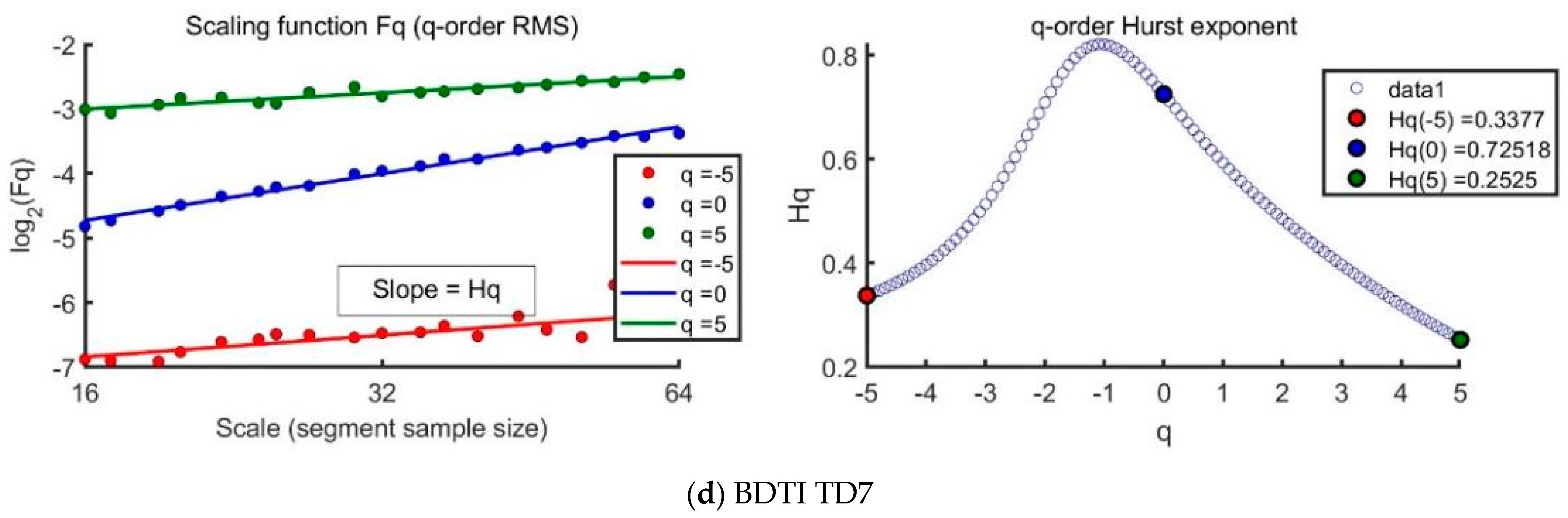
Addition of Multifractal Features: Multifractal features extracted using multifractal detrended fluctuation analysis (MFDFA) were included to capture complex market behaviors. We computed the Hurst exponent for various q-values (ranging from −5 to 5) to quantify the complexity and self-similarity within the time series.

Combination of Crisis Indicators and Multifractal Features: Both crisis indicators and multifractal features were included to examine their combined effect on prediction accuracy.

To optimize the performance of the machine learning models, we conducted a systematic hyperparameter tuning process for each base learner. Hyperparameter tuning was performed using a grid search combined with K-fold cross-validation to identify the best combination of parameters that minimized overfitting and maximized model performance. For each model, we defined a search space for key parameters, such as n_estimators, learning_rate, max_depth, and regularization terms, and evaluated different combinations using cross-validation. This process helped ensure that the selected hyperparameters were optimal for achieving robust and accurate predictions.

To combine these features for predicting Brent oil prices, we employed a stacking regression model consisting of the following base learners:

XGBoost: Capable of handling high-dimensional feature spaces and mitigating overfitting, XGBoost was used with 300 estimators, a learning rate of 0.01, and a maximum depth of 3.

LightGBM: Known for its efficient handling of large datasets, LightGBM was configured similarly to XGBoost to provide complementary strengths in feature learning.

CatBoost: Particularly effective in dealing with categorical features and reducing pre-processing requirements, CatBoost was employed with 300 iterations and a learning rate of 0.01.

The predictions from these base learners were then integrated using a Ridge Regression model as the meta-learner. This stacking approach allows the model to capture a diverse range of data patterns and interactions, thereby improving the robustness of predictions.

To provide a measure of uncertainty in the predictions, we calculated 95% confidence intervals for the predicted Brent oil prices. These intervals were derived using bootstrap resampling, offering a range within which the true values are likely to fall with 95% certainty.

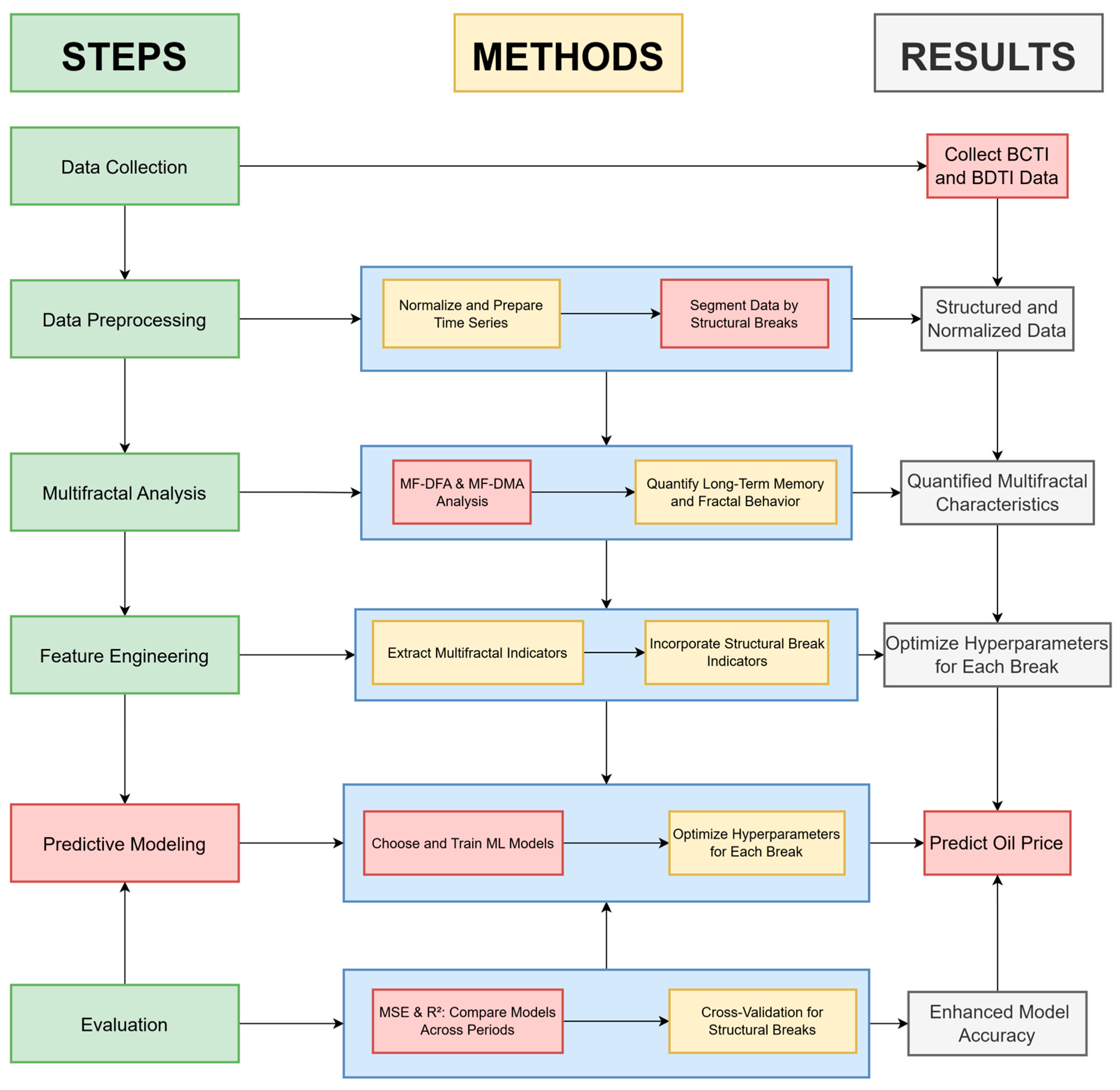
To provide a clear visual representation of the methodology, the following flowchart in Figure 1 outlines the framework for multifractal analysis and predictive modeling, which uses the Baltic Dirty Tanker Index (BDTI) and its application to Brent crude oil price prediction.

3. Data Description

The Baltic Clean Tanker Index (BCTI) is a widely tracked benchmark that measures the cost of shipping clean petroleum products, such as refined oil, on specific routes within the Baltic region [2,7,10,14]. It serves as a vital indicator for gauging freight rates and understanding the supply and demand dynamics within the clean tanker market. The BCTI’s fluctuations influence various economic sectors, making it an essential tool for industry stakeholders, analysts, and investors seeking insights into energy market trends and shipping conditions. Therefore, we pay great attention to the BCTI and specific route of TC2 from the Continent to USAC with a clean tanker size of 37,000 mt. Similarly, the Baltic Dirty Tanker Index (BDTI) serves as a key indicator for understanding freight rates and evaluating the supply and demand dynamics within the dirty tanker market. A specific route of TD7 from the North Sea to the Continent with a dirty tanker size of 80,000 mt is selected for analysis.

The sample for daily BCTI and BDTI covers the period from 28 January 1998 to 12 January 2024. The sample size includes 6413 and 6358 points, respectively, which is enough for multifractal models [36,37,38,39,40,41]. However, the data for BCTI TC2 comprise 5014 points, as the data begin from 4 March 2004. The data of BDTI TD7 include 6234 points, as we could not get the records for the year 2023. The statistical results of the sample time series are listed in

Table 4. Statistics of tanker freight rate returns.

Series\Statistics	Size	Mean	Std.	Min.	Max.
BCTI	6413	2.28 × 10−5	0.02	−0.57	0.29
BCTI TC2	5014	−2.37 × 10−4	0.04	−0.37	0.58
BDTI	6358	6.44 × 10−5	0.02	−0.38	0.24
BDTI TD7	6234	8.27 × 10−5	0.05	−0.50	0.46

. Figure 2 describes the BCTI and BDTI of the sample observations. There are big volatilities in the year 2008 under the global financial crisis, in the year 2020 when the COVID-19 broke out, and in the year 2022 when geographic conflict happened. Figure 3 records the BCTI and BDTI logarithmic changes (that is, $lnP\left(t\right)/P\left(t-1\right)$), which are widely applied to calculate daily volatilities, and the returns often help to decrease non-stationarities, though it is not required in multifractal methods [12,39].

4. Analysis of Results

4.1. Multifractality in Dirty and Clean Tanker Freight Rate Returns

The Hurst exponent serves as a metric that quantifies the expansion rate of the root-mean-square (RMS) deviation in a time series as the observational window, or scale, increases. This measure provides insights into the monofractal properties of the data [11,28,33,35]. Within the framework of a multifractal time series, localized fluctuations, or root-mean-square (RMS) deviations, tend to attain notably high magnitudes in segments that correspond to intervals of substantial volatility. Conversely, these deviations exhibit significantly lower magnitudes in segments characterized by periods of minimal fluctuation [32,33,34]. Figure 4a,d on the left illustrates that for multifractal time series, these slopes $h_q$ vary depending on the value of q. The distinction between the q-order RMS for positive and negative fluctuations is more pronounced at smaller segment widths than at larger ones. This is because smaller segments are more sensitive to local variability within a specific period, whereas larger segments encompass multiple periods and tend to average out the differences in fluctuation magnitude. As q increases, the q-order RMS for a multifractal time series generally decreases, as shown on the right side of Figure 4a,d. Both BCTI and BDTI returns exhibit multifractal characteristics, indicating that their fluctuation patterns are not uniform across different scales and require a more nuanced analysis to understand their underlying dynamics [12,43].

4.2. Multifractal Characteristics of Tanker Freight Fluctuation Under Structural Breaks

The logarithmic return of BCTI and BDTI and the specific routes in Figure 2 suggest that there were significant fluctuations in 2008, 2020, and 2022, coinciding with financial crises (COVID-19 or geographic conflict), which is in accordance with the references [7,9,12,45]. According to the references, big events such as the global financial crisis can lead to structural breaks in time series [46,47]. Therefore, we divide the sample data BDTI into two parts: Period I, from 28 January 1998 to 1 December 2010, and period II, from 2 December 2010 to 12 January 2024, to delve into the changing external factors’ effects on the multifractalities.

The study of multifractal time series often involves various scaling exponents, among which the q-order Hurst exponent $h_q$ is prominent. However, the local Hurst exponent $h_t$ has proved advantageous in detecting specific time points of structural change within a time series [47,48,49,56,57]. This local perspective aligns with q-order Hurst values $h_q$ for extreme fluctuations, correlating positively or negatively depending on the q value’s sign. The utility of the local Hurst exponent $Ht$ is particularly evident when financial time series experience sudden disturbances. It pinpoints how these shocks modify the series’ inherent scale-invariant features on a localized level [23,24,25,26,27]. Visualized through histograms, the temporal variations of the local Hurst exponent $Ht$ offer a probability distribution $Ph$ of these changes (illustrated in Figure 5e for the first period and Figure 5f for the second period). Complementing this, the multifractal spectrum—delineated by the parameters $f\left(\alpha \right)$ and $\alpha$—captures the breadth of multifractality within the series (depicted in Figure 5e for the first period and Figure 5f for the second period). An increasing spectrum breadth denotes growing structural disparities between periods marked by minor and major fluctuations [25,26,27,28]. The research employs multifractal spectrum width $\mathsf{\Delta }\alpha$ as a measure of multifractality level. The results presented in Figure 5e,f confirm strong multifractality in both examined periods of the Baltic Dirty Tanker Index (BDTI) returns. These findings align with previous research outlined in references [17,18], solidifying the observed characteristics of the market across different analytic methodologies. Figure 5a,c shows that both the BCTI and BDTI markets have multifractal characteristics, though they are different from the specific routes of TC2 and TD7 in Figure 5b,d.

4.3. Temporal Dynamics of Tanker Freight Market Complexity Using the MF-DMA Method

In Figure 6a, the multifractality from PDF is $\mathsf{\Delta }{\alpha }_{PDF}=0.48$, while the total multifractality from the three parts is $\mathsf{\Delta }\alpha =0.90$. The multifractality from linear correlation and PDF is $\mathsf{\Delta }{\alpha }_{LM}+\mathsf{\Delta }{\alpha }_{PDF}=0.61$, so the multifractality from the nonlinear correlation is $\mathsf{\Delta }{\alpha }_{NL}=0.29$. The true multifractality $\mathsf{\Delta }{\alpha }_{eff}=\mathsf{\Delta }{\alpha }_{PDF}+\mathsf{\Delta }{\alpha }_{NL}=0.77$. The results in Figure 6a–f are listed in

Table 5. MF-DMA results for tanker freight rates.

Title 1	$\mathsf{\Delta }\mathit{\alpha }$	$\mathsf{\Delta }{\mathit{\alpha }}_{\mathit{P}\mathit{D}\mathit{F}}$	$\mathsf{\Delta }{\mathit{\alpha }}_{\mathit{L}\mathit{M}}+\mathsf{\Delta }{\mathit{\alpha }}_{\mathit{P}\mathit{D}\mathit{F}}$	$\mathsf{\Delta }{\mathit{\alpha }}_{\mathit{N}\mathit{L}}$	$\mathsf{\Delta }{\mathit{\alpha }}_{\mathit{e}\mathit{f}\mathit{f}}$
BCTI	0.90	0.48	0.61	0.29	0.77
BCTI TC2	0.86	0.23	0.39	0.47	0.70
BDTI	0.58	0.28	0.52	0.06	0.34
BDTI TD7	1.03	0.28	0.50	0.53	0.81
BDTI 1998–2010	0.60	0.29	0.54	0.06	0.35
BDTI 2010–2023	0.72	0.35	0.62	0.10	0.45

.

The multifractality analysis of the Baltic Clean Tankers market in Figure 6a reveals significant insights into its dynamics. A multifractality value of 0.90 for the original data points to a highly complex market with pronounced multifractal behavior due to strong correlations at various time scales. A lesser, but still substantial, multifractality value of 0.61 in the surrogate data indicates that multifractality persists without temporal correlations, suggesting that price change distributions inherently contribute to market complexity. The shuffled data’s multifractality value at 0.48, the lowest observed, illustrates the crucial role of temporal ordering in market behavior. These values collectively attest to the market’s intricate and nonlinear interactions across scales [43].

The multifractality analysis for the Baltic Clean Tankers in Figure 6a,b, inclusive of the specific 37,000 tonnage route, elucidates distinct market dynamics. The original data for the entire market and the targeted route yield high multifractality values of 0.9 and 0.86, respectively, underscoring considerable multifractal behavior. However, subsequent surrogate and shuffled data yield diminished multifractality values of 0.61 and 0.48 for the broader market, and 0.39 and 0.23 for the specific route, respectively. These reductions upon data modification suggest inherent temporal organization as a key contributor to multifractality [26,27,28,43]. The analysis underscores the influence of data structure on the assessment of market complexity and multifractal characteristics.

The multifractal analysis of the Baltic Dirty Tankers market data in Figure 6c reveals varying degrees of market complexity. An original multifractality value of 0.58 indicates a moderately complex market structure with self-similarity across time scales. The surrogate data’s 0.52 multifractality value suggests that nontrivial scaling behavior persists even after the removal of some structural correlations. This denotes inherent complexity within the price change distribution itself [14,26,27,28]. A notably lower multifractality value of 0.28 in the shuffled data emphasizes the importance of chronological order, indicating that temporal organization significantly contributes to the market’s multifractal nature [43].

The multifractal analysis for the Baltic Dirty Tankers market on a specific route TD7 at the 80,000-tonnage level in Figure 6d exhibits a high degree of market complexity, with original data yielding a multifractality value of 1.03. This denotes a rich multifractal structure and extensive self-similarity across temporal scales. Upon surrogate treatment, multifractality is markedly reduced to 0.5, indicating diminished multifractal behavior upon the exclusion of certain structural and temporal correlations. Further declines to a multifractality value of 0.28 in the shuffled data underscore the pivotal role of temporal sequencing in fostering multifractal properties.

4.4. Predictive Applications: Using BDTI to Predict Brent Oil Prices

4.4.1. Understanding Complexity for Specific Periods and Motivation for Predictive Modeling

The comparative assessment of the Baltic Dirty Tankers from the specified periods of 1998 to 2010 and 2010 to 2023 in Figure 6e,f can provide valuable insights into the temporal changes in multifractal nature and complexity within the market dynamics. The original multifractality value of 0.72 in the first period decreases to 0.60, suggesting a potential reduction in complexity and multifractal behavior. For the period of 1998 to 2010, the surrogate data yield a multifractality value of 0.62, indicating a decrease in complexity compared to the original data, similar to the period from 2010 to 2023. The shuffled data provide additional insights into the temporal changes in multifractality [26,43]. For the period of 1998 to 2010, the shuffled data yield a multifractality value of 0.35, reflecting a notable reduction in complexity compared to the original and surrogated data. Likewise, for the period from 2010 to 2023, the value further decreases to 0.29, signaling a continued decrease in complexity during the later period. Overall, the period from 2010 to 2023 exhibits higher multifractality values across all data types, indicating a stronger multifractal nature and greater complexity [16,26,27,28].

These findings prompted our interest in understanding the underlying driving factors behind this marked increase in market complexity post-2010. To gain deeper insights, we apply a novel predictive approach using freight rates (BDTI) to predict Brent oil prices during distinct periods, aiming to explore the predictive power of freight rates in different market phases.

4.4.2. Predictive Results and Analysis for Periods I–IV

In this section, we focus on predicting Brent oil prices for the four key periods identified in Section 2.5. These periods include Period I (1 January 2006 to 31 December 2010) during the 2008 global financial crisis, Period II (30 June 2013 to 30 June 2016) amid the 2014 Shale Oil Revolution, Period III (1 January 2019 to 1 January 2021) during the COVID-19 crisis, and Period IV (1 January 2021 to 12 January 2024) following the 2022 Russia–Ukraine conflict. The predictive process begins with the Baltic Dirty Tanker Index (BDTI) as the main feature, along with additional features that were introduced in Section 2.5.

The resulting predictions for Periods I–IV are illustrated in Figure 7–10, where multiple models are compared against the actual Brent oil prices. The models include

Predicted_Direct: Predictions made using only BDTI data.

Predicted_Time_Indicator: Incorporating the crisis time indicator to assess the effect of the COVID-19 pandemic.

Predicted_Multifractal: Including multifractal features derived from the BDTI to understand the impact of market complexity.

Predicted_Multifractal_Indicator: Utilizing both the crisis indicator and multifractal features to determine their combined influence.

In Period I, the 2008 global financial crisis had a profound effect on both freight rates and oil prices. Figure 7 shows the predictive results, indicating that the inclusion of multifractal features and crisis indicators significantly improved prediction accuracy compared to the direct approach.

In Period II, during the 2014 Shale Oil Revolution, the predictive model that included multifractal features outperformed the direct prediction, as shown in Figure 8. The Predicted_Multifractal_Indicator model captured the complex fluctuations caused by shifts in the energy supply landscape more effectively.

In Period III, the COVID-19 pandemic triggered unprecedented volatility in global markets, significantly impacting freight rates and oil prices. Figure 9 shows that incorporating both crisis indicators and multifractal features markedly improved prediction accuracy compared to the direct approach. Notably, the Predicted_Multifractal_Indicator model effectively captured the rapid market fluctuations during the early stages of the pandemic, demonstrating robust performance under extreme volatility.

Finally, in Period IV, the 2022 Russia–Ukraine conflict introduced significant geopolitical uncertainty. As shown in Figure 10, the Predicted_Multifractal_Indicator model once more achieved the most accurate fit, characterized by diminished error margins and a closer correspondence to actual price fluctuations. This outcome underscores the utility of incorporating multifractal features into the model, particularly during periods marked by elevated volatility.

Overall, although the Predicted_Direct model exhibits noticeable discrepancies during periods of elevated volatility, integrating multifractal features in the Predicted_Multifractal approach significantly enhances the model’s capacity to capture complex market dynamics. As a result, the forecasts better align with actual price movements. Moreover, the Predicted_Multifractal_Indicator model refines these predictions further by incorporating both the crisis indicator and the multifractal features, consistently achieving the closest fit across all four periods.

4.4.3. Robustness Analysis of Prediction Methods

Above, we presented several intuitive figures that provide a visual comparison of the predictive performance of different models across the four periods. Now, we proceed to a more detailed quantitative analysis to corroborate these visual observations with empirical metrics. Specifically, we focus on the predictive accuracy as measured by the (MSE) and R² values, which offer critical insights into the effectiveness of incorporating multifractal features and crisis indicators into the forecasting models.

Table 6. MSE values for training and test sets across Periods I–IV.

		Period I	Period II	Period III	Period IV
Direct Prediction	Train MSE	185.91	557.19	82.25	90.88
	Test MSE	186.12	539.10	114.72	114.66
Prediction with Crisis Period Indicator	Train MSE	104.45	422.13	65.49	35.46
	Test MSE	109.53	400.39	71.48	39.55
Prediction with MFDFA Features	Train MSE	56.50	40.61	13.09	20.47
	Test MSE	72.90	56.82	25.93	35.69
Prediction with Indicator and MFDFA	Train MSE	49.85	35.80	9.16	12.18
	Test MSE	62.19	40.76	15.82	16.76

presents the mean squared error (MSE) values for both the training and test sets across all periods, demonstrating the improvement in predictive accuracy after incorporating multifractal features. As shown in the figure, the inclusion of these features significantly reduces the MSE values across all four periods, with the greatest improvements observed in Periods II, III, and IV. This suggests that the predictive models benefited substantially from the added complexity of multifractal characteristics, especially in the post-2010 periods, when market dynamics became increasingly intricate.

Table 7. R² scores for training and test sets across Periods I–IV.

		Period I	Period II	Period III	Period IV
Direct Prediction	Train R2	0.53	0.34	0.49	0.54
	Test R2	0.52	0.35	0.40	0.50
Prediction with Crisis Period Indicator	Train R2	0.73	0.50	0.59	0.82
	Test R2	0.72	0.52	0.62	0.83
Prediction with MFDFA Features	Train R2	0.86	0.95	0.92	0.90
	Test R2	0.81	0.93	0.86	0.85
Prediction with Indicator and MFDFA	Train R2	0.87	0.96	0.94	0.94
	Test R2	0.84	0.95	0.92	0.93

displays the R² scores for both the training and test sets, providing insights into the proportion of variance explained by the models. Predictive models with multifractal features exhibit substantially higher R² values compared to direct prediction models. Specifically, for Periods II, III, and IV, the Predicted_Multifractal_Indicator model achieves R² values close to or exceeding 0.9, indicating a strong fit to the actual data. Interestingly, the enhancement in predictive performance is less pronounced for Period I, suggesting that the multifractal characteristics during this earlier period were less influential compared to the more recent periods. This aligns with our previous observations that post-2010 periods exhibited greater multifractality and complexity, thereby benefiting more from the incorporation of multifractal features.

To provide a more comprehensive understanding, Figure 11 and

Table 8. Percentage improvements in MSE and R² with multifractal features in predictive models across Periods I–IV.

	Period I	Period II	Period III	Period IV
Train MSE	69.61%	92.71%	84.09%	77.48%
Test MSE	60.83%	89.46%	77.40%	68.87%
Train R2	62.65%	182.54%	88.60%	66.16%
Test R2	55.20%	167.62%	117.14%	68.28%

illustrates the substantial percentage improvements in MSE and R² when multifractal features are incorporated into the predictive models for each period. For instance, during Period II, the R² for training improves by approximately 182.54%, and the R² for testing by 167.62%, highlighting a dramatic enhancement in model performance when multifractal features are added. Similarly, Period III shows an 88.60% improvement in training R² and a 117.14% increase in testing R², emphasizing the importance of capturing complex dynamics during high volatility phases, such as those triggered by the COVID-19 pandemic. Notably, the improvements in Periods II, III, and IV are significantly greater compared to Period I, which only shows modest gains, reinforcing the notion that market dynamics after 2010 became more intricate and multifaceted. This distinct difference in performance can be attributed to increased globalization, advancements in technology, and heightened geopolitical sensitivity after 2010, all contributing to more complex and unpredictable market interactions. These findings underscore that the multifractal characteristics are especially relevant for capturing the nuances of post-2010 market behavior, making the predictive models significantly more effective for later periods.

Such findings are critical as they highlight the evolving nature of the oil market and underscore the importance of adapting predictive methodologies to account for changes in market structure and dynamics. The enhanced performance of models that integrate multifractal characteristics, particularly during times of increased market complexity, suggests that conventional linear models may lack the capacity to fully capture the intricate dynamics of contemporary financial markets. By utilizing multifractal analysis, stakeholders can achieve a deeper understanding of market dynamics and enhance their decision-making processes, particularly during times of instability.

5. Discussion of Results

From the discussion, one may conclude that this study successfully unravels the multifaceted complexity of the Baltic Tanker Freight market using multifractal analysis techniques and advanced machine learning models. By integrating the Baltic Dirty Tanker Index (BDTI) as a leading indicator, we demonstrate that freight rates can effectively predict Brent oil prices, particularly during heightened market volatility caused by global crises, such as the 2008 financial crisis, the 2014 Shale Oil Revolution, the COVID-19 pandemic, and the Russia–Ukraine conflict. The findings reveal that multifractal characteristics, such as the generalized Hurst exponent and multifractal spectrum, significantly enhance the predictive accuracy of the models, outperforming traditional approaches that rely solely on linear or unidirectional relationships [7,8,9]. Moreover, the stacking regression framework combining XGBoost, LightGBM, CatBoost, and Ridge Regression validates the robustness of the proposed methodology, aligning closely with contemporary machine learning advancements [26,58,60]. These results provide actionable insights for policymakers, energy companies, and investors, emphasizing the utility of multifractal analysis in managing systemic risks and navigating energy market volatility [4,5,6].

5.1. Resolution and Discussion of Key Research Questions

The results indicate that the multifractal complexity of the tanker freight market intensified over time, particularly after 2010. The expansion of the multifractal spectrum width suggests a shift from crisis-driven volatility to a market increasingly shaped by regulatory changes, technological advancements, and macroeconomic dynamics. Beyond these general factors, our findings reveal that major external shocks—such as the 2008 global financial crisis, the 2014 Shale Oil Revolution, the COVID-19 pandemic, and the Russia–Ukraine conflict—each introduced distinct structural changes in market behavior, further reinforcing the role of multifractal analysis in capturing such transformations. The increasing multifractality implies that systemic risks have grown, as heightened market complexity makes price movements more sensitive to external shocks. These findings highlight the evolving nature of the freight market and underscore the necessity of adaptive risk management strategies to mitigate the effects of rising uncertainty.

Furthermore, temporal correlations and volatility play a significant role in shaping market dynamics. The MF-DFA and MF-DMA analyses show that long-range dependencies and nonlinear patterns are evident in the freight rate time series, influencing both short-term fluctuations and long-term trends. The Hurst exponent confirms that persistent correlations are present, suggesting that freight rate changes are not purely random but follow structured patterns across different time scales. Additionally, decomposing multifractal properties reveal that both nonlinear dependencies and heavy-tailed distributions contribute to market complexity. These results reinforce the importance of incorporating multifractal analysis alongside traditional econometric models to improve market forecasting and risk assessment.

The role of external shocks and structural shifts is also evident in the analysis. Significant global events, such as the 2008 financial crisis, the 2014 Shale Oil Revolution, the COVID-19 pandemic, and the Russia–Ukraine conflict, have introduced structural breaks and heightened multifractal behavior. For instance, the financial crisis caused abrupt market contractions, while the Shale Oil Revolution led to fundamental shifts in supply–demand balances. The COVID-19 pandemic resulted in extreme volatility due to unprecedented supply chain disruptions, and the Russia–Ukraine conflict further exacerbated oil price instability. These findings suggest that external shocks not only increase short-term volatility but also contribute to long-term changes in market complexity, highlighting the need for more adaptive analytical techniques.

The predictive utility of the Baltic Dirty Tanker Index (BDTI) in forecasting Brent oil prices is particularly evident during periods of heightened market uncertainty. While traditional models often assume that oil prices drive freight rates, the results suggest that freight rates, influenced by supply chain dynamics and macroeconomic conditions, can serve as leading indicators of oil price movements [17,18]. The inclusion of multifractal characteristics, such as the Hurst exponent and multifractal spectrum, significantly improves forecast accuracy, especially during market turbulence. This highlights the advantages of integrating multifractal features into predictive models to better capture the nonlinearity and evolving structure of global energy markets.

5.2. Guiding Energy Market Decisions Through Predictive Insights

The findings of this study provide actionable insights for investors, energy companies, and policymakers, particularly in managing risks and making strategic decisions during periods of economic and geopolitical instability. Investors can use the predictive framework to anticipate oil price fluctuations, adjust portfolios, and optimize trading strategies. For example, during market disruptions, such as the 2008 financial crisis or the 2022 Russia–Ukraine conflict, early signals from freight rate trends could help investors mitigate exposure to volatile price swings. Energy companies can integrate these insights into hedging strategies, contract negotiations, and operational planning. By leveraging freight rate-based predictions, firms can proactively adjust chartering and fuel procurement strategies to minimize cost fluctuations and supply chain risks.

Policymakers can utilize these findings to enhance market stability by incorporating freight rate indicators into early warning systems. Predictive insights can help regulators anticipate disruptions in the energy supply chain and implement timely interventions, such as adjusting strategic petroleum reserves or introducing temporary regulatory measures. By demonstrating the predictive value of freight indices and the power of multifractal analysis, this study offers a practical framework for industry stakeholders to navigate the complexities of the global energy market with greater confidence and strategic foresight.

5.3. Additional Considerations and Future Directions

While the proposed framework demonstrates strong predictive capability, an important question remains: To what extent can the model generalize beyond the Baltic Dirty Tanker Index (BDTI)? The BDTI serves as a key indicator within the tanker freight market, yet future research should assess whether similar multifractal properties extend to other freight indices, such as the Baltic Clean Tanker Index (BCTI) or liquefied natural gas (LNG) freight rates. If these indices exhibit similar complexity patterns, it would reinforce the broader applicability of the methodology across various maritime and energy markets. Additionally, expanding the dataset to include diverse market indicators, such as global trade volumes, bunker fuel prices, and macroeconomic indicators, may further enhance predictive robustness and applicability.

Furthermore, while our model effectively captures major macroeconomic and geopolitical disruptions, regulatory and policy changes represent an additional dimension of uncertainty that warrants further exploration. The implementation of environmental regulations, such as the IMO 2020 sulfur cap, has introduced significant cost adjustments in the shipping industry, altering freight rate structures. Similarly, carbon pricing policies and regional emission trading schemes could further influence market behavior. Future research could incorporate such policy-driven variables into predictive modeling frameworks, enabling more comprehensive assessments of regulatory impacts on energy and freight markets.

In addition, an important consideration in financial and energy market forecasting is how to further enhance the predictive power of multifractal analysis. While this study successfully integrates machine learning models, deeper insights may be gained by leveraging advanced deep learning techniques that can dynamically adapt to the multifractal characteristics of the tanker freight market. Long short-term memory (LSTM) networks and transformer-based architectures, which have shown exceptional ability in capturing long-range dependencies, could be tailored to incorporate multifractal features such as the generalized Hurst exponent and multifractal spectrum. By embedding these features within attention mechanisms or hierarchical temporal modeling, deep learning methods could potentially refine the detection of structural shifts and volatility patterns in freight markets. Future studies could explore hybrid approaches that integrate deep learning techniques with multifractal feature engineering, allowing for a more adaptive and robust forecasting framework that better captures the evolving complexity of global energy markets.

While our predictive framework demonstrates strong forecasting accuracy, several challenges may arise in real-world trading applications. First, the model’s reliance on historical freight rate data means that sudden, unprecedented market disruptions—such as geopolitical crises or extreme weather events—may introduce unaccounted volatility, requiring adaptive recalibration. Second, integrating multifractal features into trading algorithms demands computational efficiency, as real-time market conditions require fast decision-making. Third, liquidity constraints in the tanker freight and oil futures markets may affect the practical execution of trading strategies based on model predictions, particularly during periods of high volatility. Addressing these challenges through adaptive learning techniques, real-time data integration, and further testing under different market conditions would enhance the robustness and practical applicability of the proposed approach.

Despite these contributions, it is important to acknowledge the inherent limitations of our approach. While the predictive models exhibit high accuracy, they remain reliant on historical data patterns, which may not always generalize to unprecedented market conditions. The emergence of unforeseen economic or geopolitical shocks could introduce structural changes that require continuous model adaptation. Future research should explore adaptive forecasting techniques that integrate real-time data streams, such as satellite-based vessel tracking or high-frequency trading data, to enhance responsiveness to rapid market shifts.

In conclusion, this study demonstrates the significant potential of multifractal analysis and machine learning in accurately forecasting energy prices during periods of high volatility. The findings not only advance the theoretical understanding of tanker freight markets, but also provide practical tools for stakeholders to manage uncertainty and enhance decision-making. By successfully integrating multifractal features and advanced predictive models, this study offers a robust framework that can serve as a foundation for future research. Moving forward, further refinements and broader applications of the proposed methodology may uncover additional insights into the intricate relationships shaping global energy markets, paving the way for more resilient and adaptive forecasting strategies.

6. Conclusions

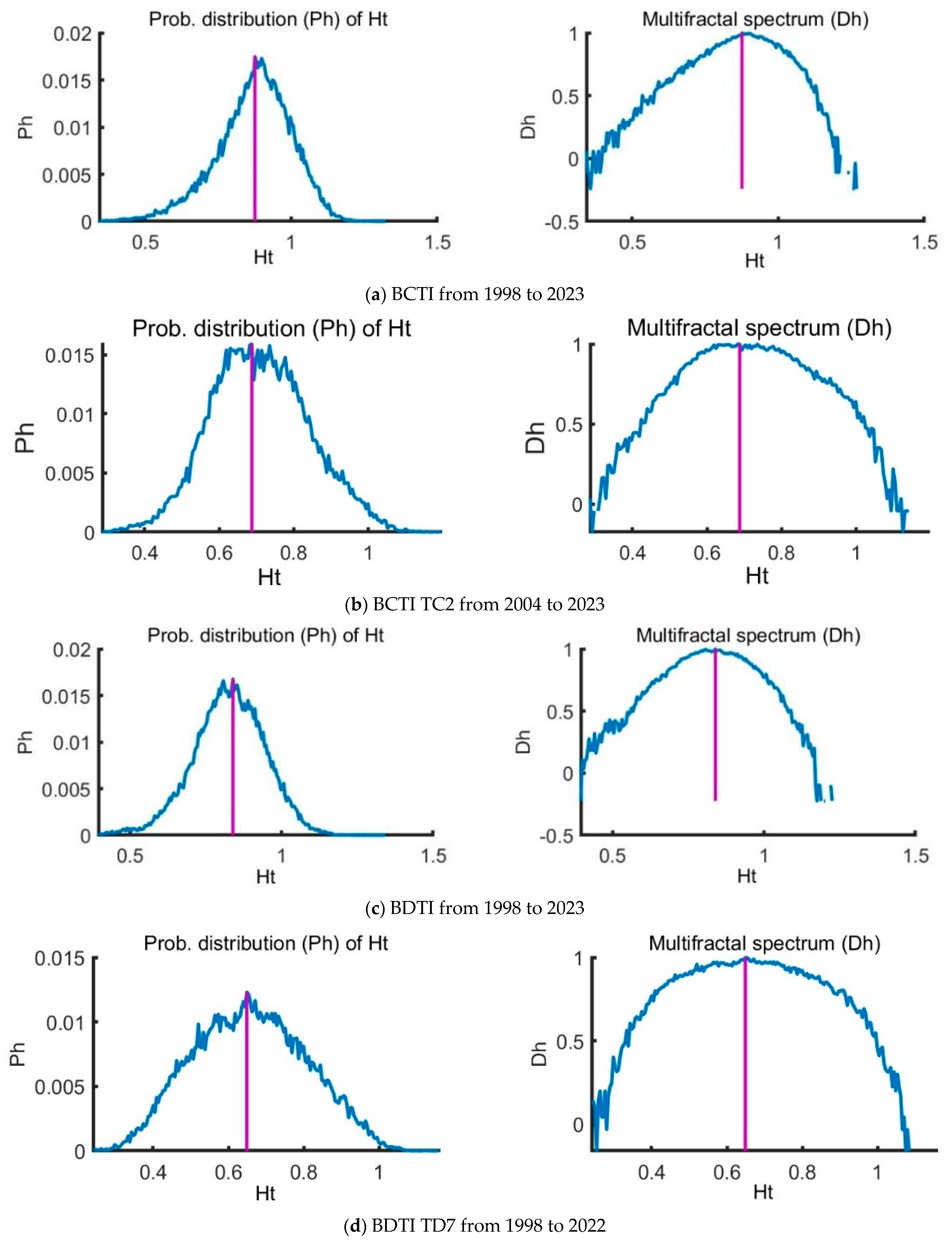
This study employs MF-DMA to analyze the Baltic tanker freight market. The findings reveal a strong multifractal structure, with total multifractality reaching 0.90 in the clean tanker market, driven by a fat-tailed probability distribution (0.48) and nonlinear correlations (0.29). Analysis of the TC2 route (37,000 ton) confirms its multifractal nature, though reduced after shuffling and surrogating, highlighting the role of temporal structure. The clean tanker market reflects a tight supply–demand balance, with freight rates responding sharply to external factors.

For dirty tankers, the study identifies moderate complexity, with multifractality at 0.58, decreasing under surrogate and shuffled conditions. In the TD7 route (80,000 ton), multifractality peaks at 1.03 but declines when temporal and structural correlations are removed, confirming the impact of chronological sequencing.

The comparison of multifractal dynamics between 1998–2010 and 2010–2024 reveals notable differences in market behavior, reflecting the influence of technological, regulatory, and environmental factors.

Based on these findings, this study establishes a predictive framework integrating BDTI, multifractal features, and crisis indicators to forecast Brent oil prices. Analysis of four major global events—the 2008 financial crisis, the 2014 Shale Oil Revolution, COVID-19, and the Russia–Ukraine conflict—demonstrates how external factors shape market dynamics. Using stacking regression (XGBoost, LightGBM, CatBoost, and Ridge Regression) enhances predictive accuracy, reinforcing the role of freight rates as leading indicators in energy markets.

This study provides strong empirical evidence that tanker freight rates, particularly the Baltic Dirty Tanker Index (BDTI), can serve as leading indicators for Brent oil prices. While conventional economic models often assume that oil prices drive freight rates, our results indicate that freight rates, shaped by supply chain dynamics and macroeconomic shifts, contain valuable predictive signals for oil prices. By leveraging the multifractal properties of freight indices, the proposed model significantly improves prediction accuracy, particularly during periods of heightened market uncertainty. The findings highlight the potential of incorporating maritime freight market signals into broader energy market forecasting models.

Multifractal analysis enhances machine learning-based forecasting methods by providing a more refined understanding of market dynamics, particularly in capturing nonlinear patterns and structural shifts. By incorporating multifractal features such as the Hurst exponent and multifractal spectrum, the predictive framework improves the ability to recognize variations in market complexity over different time periods. This approach complements traditional forecasting models by offering deeper insights into the evolving nature of financial time series, especially in the tanker freight and oil markets. The results indicate that integrating multifractal characteristics helps refine model predictions, improving stability and reducing errors, particularly during periods of heightened volatility and structural transitions.

In conclusion, this study combines multifractal analysis and predictive modeling to provide a comprehensive framework for understanding and navigating the complexities of the Baltic tanker freight market. By revealing the evolving multifractal dynamics and demonstrating the predictive power of freight rates, the research underscores the importance of integrating multifractal characteristics into forecasting models. The findings offer practical implications for strategic decision-making, operational resilience, and risk management in the shipping and energy industries. Subsequent research endeavors should expand upon this foundational framework by integrating additional datasets, optimizing predictive algorithms, and investigating the interactions between multifractal properties and other market indicators to further enhance prediction accuracy and application scope.