Control of Semilinear Differential Equations with Moving Singularities

Abstract

In this paper, we present a control problem related to a semilinear differential equation with a moving singularity, i.e., the singular point depends on a parameter. The particularity of the controllability condition resides in the fact that it depends on the singular point, which in turn depends on the control variable. We provide sufficient conditions to ensure that the functional determining the control is continuous over the entire domain of the parameter. Lower and upper solutions techniques combined with a bisection algorithm is used to prove the controllability of the equation and to approximate the control. An example is given together with some numerical simulations. The results naturally extend to fractional differential equations.

1. Introduction and Preliminaries

Differential equations are crucial in solving practical problems in many scientific fields, such as physics, chemistry, biology, economics, engineering, etc., modeling many real-world processes. However, the complexity of these phenomena often introduces various parameters that can significantly influence the outcome. A particularly intriguing problem in this context is identifying the parameters that ensure a specific quantity (e.g., density, energy) related to the solution of the differential equation reaches a desired value. This challenge naturally leads to a control problem.

Our study has two strong motivations.

(a) 

The first motivation concerns differential equations with moving singularities, which frequently appear in nonlinear models from applied sciences, such as physics and mathematical biology [1].

(b) 

The second one relates to the control of such models, aiming to reach a desired state of the process. For example, if the state variable represents a density, one might be interested in controlling its cumulative value or average. This corresponds precisely to our control problem in Section 2.

Mathematical models expressed through equations with singularities include the Briot–Bouquet equation, which has applications in complex analysis, specifically in the theory of univalent functions; equations arising in Michaelis–Menten kinetics, modeling oxygen diffusion in cells; the Thomas–Fermi equation in atomic physics; and the Emden–Fowler equation, in the study of phenomena in non-Newtonian fluid mechanics [1,2,3].

Inspired by the investigation in [4,5,6], this paper will explore the following problem:

$$\left\{\begin{array}{c}{u}^{\prime }\left(t\right)=f(t,u\left(t\right),\lambda ),t\in \left[0,\theta \left(\lambda \right)\right)\hfill \\ u\left(0\right)=u_0\left(\lambda \right).\hfill \end{array}\right.$$

(1)

Here, $f:[0,\infty )\times \mathbb{R}\times (0,\infty )\to \overline{\mathbb{R}}(:=\mathbb{R}\cup \{\pm \infty \})$ is a function that possesses a singularity in the first variable, influenced by the third one, that is, for each $\lambda >0$, there exists $\theta \left(\lambda \right)>0$, such that

$$\underset{\begin{array}{c}t\to \theta \left(\lambda \right)\\ t<\theta \left(\lambda \right)\end{array}}{lim}f(t,x,\lambda )=\pm \infty \mathrm{for}\mathrm{almost}\mathrm{all}x\in \mathbb{R}.$$

Throughout this paper, we use $u_{\lambda }$ to denote the unique solution to problem (1) for a given $\lambda >0$. Since the singularity point $\theta \left(\lambda \right)$ varies with $\lambda$, the differential Equation (1) is said to have a moving singularity.

For each $\lambda >0$, we consider the functional ${\psi }_{\lambda }:C[0,\theta \left(\lambda \right))\to \overline{\mathbb{R}}$,

$${\psi }_{\lambda }\left(u\right)={\int }_0^{\theta \left(\lambda \right)}u\left(s\right)ds,$$

(2)

where the integration over the noncompact interval $\left[0,\theta \left(\lambda \right)\right)$ is understood in the usual sense (see, e.g., [7]),

$${\int }_0^{\theta \left(\lambda \right)}u\left(s\right)ds=\underset{\begin{array}{c}t\to \theta \left(\lambda \right)\\ t<\theta \left(\lambda \right)\end{array}}{lim}{\int }_0^{t}u\left(s\right)ds.$$

Our goal in this paper is the following control problem:

Problem 1

(Control problem). Find ${\lambda }^{*}>0$ such that

$${\psi }_{{\lambda }^{*}}\left(u_{{\lambda }^{*}}\right)=p,$$

(3)

where $p\in \mathbb{R}$ is a given value.

The particularity of the controllability condition resides in the fact that it depends on the singular point, which in turn depends on the control variable. To establish sufficient conditions for the existence of a solution to this control problem, we first guarantee that the mapping $\phi :\left(0,\infty \right)\to \mathbb{R}$,

$$\phi \left(\lambda \right)={\psi }_{\lambda }\left(u_{\lambda }\right),$$

(4)

is well-defined and continuous on $(0,\infty )$. Then, we are able to use a lower and upper solution argument to guarantee the existence of a ${\lambda }^{*}$ with the desired property (3). Moreover, by the  bisection algorithm, we have a method of approximation of the value ${\lambda }^{*}.$

Control problems on a fixed interval that require one to find a parameter in order to achieve a specific controllability condition are well-documented in the literature (see, e.g., [8,9,10]). The novelty of this paper lies in determining such a parameter where each solution is defined on a different interval. This approach requires a more refined analysis and leads to more complex problems.

The main assumptions we use in our analysis are as follows:

(h1) 

For each $\lambda >0$ and $0<\epsilon <\theta \left(\lambda \right)$, there exists a constant $L=L(\lambda ,\epsilon )$, such that for all $x,\overline{x}\in \mathbb{R}$ and for all $t\in \left[0,\theta \left(\lambda \right)-\epsilon \right]$, we have

$$|f(t,x,\lambda )-f(t,\overline{x},\lambda )|\le L(\lambda ,\epsilon )|x-\overline{x}|.$$

(h1) 

The mappings

$$\lambda \mapsto \theta \left(\lambda \right),\lambda \mapsto u_0\left(\lambda \right),\lambda \mapsto L(\lambda ,\epsilon )(\mathrm{for}\mathrm{each}\epsilon >0),$$

are continuous. Additionally, the map $(t,x,\lambda )\mapsto f(t,x,\lambda )$ is continuous for $t\in [0,\theta (\lambda \left)\right)$, $x\in \mathbb{R}$, and $\lambda \in (0,\infty )$.

In the next lemma, we show that assumptions (h1) and (h2) are sufficient to guarantee the existence of a unique solution of problem (1).

Lemma 1.

Under assumptions (h1) and (h2), for each $\lambda >0$ there exists a unique solution $u_{\lambda }\in C[0,\theta \left(\lambda \right))$ of problem (1). Moreover, this solution satisfies the integral equation

$$u_{\lambda }\left(t\right)=u_0\left(\lambda \right)+{\int }_0^{t}f(s,u_{\lambda }\left(s\right),\lambda )ds,$$

(5)

for all $t\in \left[0,\theta \left(\lambda \right)\right).$

Proof. 

Let $\lambda >0$. For each $0<\epsilon <\theta \left(\lambda \right)$, we consider the initial value problem on the cut-off domain,

$$\left\{\begin{array}{cc}{u}^{\prime }\left(t\right)=f(t,u\left(t\right),\lambda ),\hfill & t\in \left[0,\theta \left(\lambda \right)-\epsilon \right]\hfill \\ u\left(0\right)=u_0\left(\lambda \right).\hfill \end{array}\right.$$

(6)

From assumption (h1), the mapping $x\mapsto f(t,x,\lambda )$ is Lipschitz continuous with the Lipschitz constant $L_{\lambda ,\epsilon }$. Therefore, problem (6) has a unique solution (see, e.g., [11,12]). The conclusion follows immediately by letting $\epsilon \to 0$ and using the uniqueness of the solution on each interval $[0,\theta (\lambda )-\epsilon ]$. Relation (5) can be easily deduced by taking the integral in (1) from 0 to $t.$    □

Example 1.

The model for $f(t,x,\lambda )$ is given by

$$f(t,x,\lambda )={\displaystyle \frac{x}{\lambda -t}}.$$

Clearly, there is a singularity at $\theta \left(\lambda \right)=\lambda$. However, when the first variable is restricted to a compact interval $[0,\lambda -\epsilon ]$ with $0<\epsilon <\theta \left(\lambda \right)$, the function f is Lipschitz continuous with $L(\lambda ,\epsilon )={\displaystyle \frac{1}{\epsilon }}$ the Lipschitz constant. If we set $u_0\left(\lambda \right)={\displaystyle \frac{1}{\lambda }}>0$, the unique solution of the problem (1) is

$$u_{\lambda }\left(t\right)={\displaystyle \frac{1}{\lambda -t}},\mathrm{for}\mathrm{all}t\in [0,\lambda ).$$

Remark 1.

Without imposing further assumptions beyond (h1) and (h2), we cannot generally expect φ to be well-defined and continuous on $(0,\infty )$. For instance, consider the case where

$$f(t,x,\lambda )={\displaystyle \frac{1}{\lambda {(\lambda -t)}^{\frac{1}{\lambda }+1}}}\mathrm{and}{u}_0\left(\lambda \right)={\displaystyle \frac{1}{{\lambda }^{1/\lambda }}}.$$

Clearly, both assumptions (h1) and (h2) are satisfied. Straightforward calculations yield

$$u_{\lambda }\left(t\right)={(\lambda -t)}^{-{\displaystyle \frac{1}{\lambda }}},$$

for each $\lambda >1$. Consequently,

$$\phi \left(\lambda \right)={\displaystyle \frac{1}{\lambda -1}}{\lambda }^{{\displaystyle \frac{2\lambda -1}{\lambda }}}.$$

This implies that $\phi \left(\lambda \right)\in \mathbb{R}$ for $\lambda >1$, but 

$$\underset{\begin{array}{c}\lambda \to 1\\ \lambda >1\end{array}}{lim}\phi \left(\lambda \right)=\infty .$$

The paper is structured as follows: Section 2 presents the original results on the controllability of equations with moving singularities. Before establishing the main result (Theorem 6), we derive several auxiliary results concerning the continuous dependence of solutions on the control parameter and the continuity of the control functional with respect to the control variable. In Section 3, we provide a theoretical algorithm for obtaining the solution of the control problem using the method of lower and upper solutions. We also provide an example that illustrates the applicability of the obtained results. Finally, in Section 4 we suggest a possible extension of our approach to fractional differential equations with moving singularities.

In the following, we present some well-known results from the literature that will be used throughout this paper. The first result is the Arzelà–Ascoli theorem (see, e.g., [13,14]).

Theorem 1

(Arzelà–Ascoli theorem). A subset $F\subset \left({C[a,b],|·|}_{\infty }\right)$, where ${|·|}_{\infty }$ is the supremum norm, is relatively compact if and only if it is uniformly bounded and equicontinuous, that is, there exists $M>0$ with

$${\left|u\right|}_{\infty }\le M,forallu\in F,$$

and for every $\epsilon >0$, there exists $\delta \left(\epsilon \right)>0$ such that

$$\left|u\left(x\right)-u\left(y\right)\right|\le \epsilon ,forx,y\in [a,b]with\left|x-y\right|\le \delta \left(\epsilon \right)andallu\in F.$$

The next lemma provides an alternative condition to ensure the convergence of a sequence based on the behavior of its sub-sequences (see, e.g., [15] (Lemma 1.1)).

Theorem 2.

Let X be a topological space, and let $\left(x_n\right)$ be a sequence in X with the following property: there exists $x\in X$, such that, from any sub-sequences of $\left(x_n\right)$, a further sub-sequences can be extracted that converges to x. Then, the entire sequence $\left(x_n\right)$ converges to x.

Finally, we have the well-known Grönwall’s lemma (see, [16,17]).

Theorem 3

(Grönwall inequality). Let $u,v\in C[a,b]$. If there exists a constant $c>0$ such that

$$\left|u\left(t\right)\right|\le c+{\int }_a^t\left|u\left(s\right)\right|\left|v\left(s\right)\right|dsfort\in [a,b],$$

then

$$\left|u\left(t\right)\right|\le cexp\left({\int }_a^t\left|v\left(s\right)\right|ds\right)fort\in [a,b].$$

2. Auxiliary Lemmas and New Controllability Result

2.1. Proprieties of the Solutions $u_{\lambda }$

In this section, we present some properties of the solutions to problem (1), which will be used later in our analysis.

Lemma 2.

Assume that assumptions (h1) and (h2) hold. Then, given any sequence of positive real numbers $\left({\lambda }_k\right)$ converging to some ${\lambda }^{*}>0$, the sequence of solutions $\left(u_{{\lambda }_k}\right)$ converges uniformly to $u_{{\lambda }^{*}}$ on any interval $[0,\theta \left({\lambda }^{*}\right)-\epsilon ]$, with $0<\epsilon <min\left\{{inf}_{k\in \mathbb{N}}\theta \left({\lambda }_k\right),\theta \left({\lambda }^{*}\right)\right\}$.

Proof. 

Let $\left({\lambda }_k\right)$ be a sequence of positive real numbers with ${\lambda }_k\to {\lambda }^{*}>0$ as $k\to \infty$, and let

$$0<\epsilon <min\left\{\underset{k\in \mathbb{N}}{inf}\theta \left({\lambda }_k\right),\theta \left({\lambda }^{*}\right)\right\}.$$

(7)

Since the mapping $\lambda \mapsto \theta \left(\lambda \right)$ is continuous, there exists $k_0\in \mathbb{N}$, such that

$$\theta \left({\lambda }^{*}\right)-\epsilon \le \theta \left({\lambda }_k\right)-{\displaystyle \frac{\epsilon }{2}},$$

for all $k\ge k_0$. Clearly, the choise of $\epsilon$ given in guarantees that both $\theta \left({\lambda }^{*}\right)-\epsilon$ and $\theta \left({\lambda }_k\right)-{\displaystyle \frac{\epsilon }{2}}$ are strictly positive, for all $k\ge k_0.$

Using condition (h1), for each $k\ge k_0$, there exists $L\left({\lambda }_k,{\displaystyle \frac{\epsilon }{2}}\right)>0$, such that

$$\left|f\left(t,x,{\lambda }_k\right)-f\left(t,\overline{x},{\lambda }_k\right)\right|\le L\left({\lambda }_k,{\displaystyle \frac{\epsilon }{2}}\right)\left|x-\overline{x}\right|$$

for all $t\in [0,\theta \left({\lambda }_k\right)-\epsilon ]$ and all $x,\overline{x}\in \mathbb{R}$. Moreover, from the continuity of the mapping $\lambda \mapsto L\left(\lambda ,{\displaystyle \frac{\epsilon }{2}}\right)$, there exists a positive real number $\overline{L}>0$, such that

$$L\left({\lambda }_k,{\displaystyle \frac{\epsilon }{2}}\right)\le \overline{L}\mathrm{for}\mathrm{all}k\ge k_0.$$

Furthermore, using the Arzelà–Ascoli theorem, we show that the set

$$A:=\left\{u_{{\lambda }_k}:[0,\theta \left({\lambda }^{*}\right)-\epsilon ]\to \mathbb{R},k\ge k_0\right\}$$

is relatively compact in $C[0,\theta \left({\lambda }^{*}\right)-\epsilon ]$. First, we establish the uniform boundedness of the set A. Let $k\ge k_0$ and let $t\in [0,\theta \left({\lambda }^{*}\right)-\epsilon ]$. Using the integral form (5) of $u_{{\lambda }_k}$, we obtain

$$\begin{array}{ccc}\hfill \left|u_{{\lambda }_k}\left(t\right)\right|& \le & \left|u_0\left({\lambda }_k\right)\right|+{\int }_0^t\left|f(s,u_{{\lambda }_k}\left(s\right),{\lambda }_k)-f(s,0,{\lambda }_k)\right|ds+{\int }_0^t\left|f(s,0,{\lambda }_k)\right|ds\hfill \\ & \le & \left|u_0\left({\lambda }_k\right)\right|+{\int }_0^t{e}^{s\rho }{e}^{-s\rho }\overline{L}\left|u_{{\lambda }_k}\left(s\right)\right|ds+{\int }_0^t\left|f(s,0,{\lambda }_k)\right|ds\hfill \\ & \le & {\left|u_{{\lambda }_k}\right|}_{\rho }{\displaystyle \frac{\overline{L}}{\rho }}{e}^{t\rho }+M,\hfill \end{array}$$

(8)

where

$${\left|u\right|}_{\rho }=\underset{t\in [0,\theta \left({\lambda }^{*}\right)-\epsilon ]}{sup}{e}^{-t\rho }\left|u\left(t\right)\right|,$$

is the Bielecki norm on $C[0,\theta \left({\lambda }^{*}\right)-\epsilon ]$, and 

$$M=\underset{k\ge k_0}{sup}\left(\left|u_0\left({\lambda }_k\right)\right|+{\int }_0^{\theta \left({\lambda }^{*}\right)-\epsilon }\left|f\left(s,0,{\lambda }_k\right)\right|ds\right).$$

Note that $M<\infty$. Indeed, the continuity of the mapping $(t,\lambda )\mapsto f(t,0,\lambda )$ guarantees that it is uniformly bounded on the compact set

$$(t,\lambda )\in \left[0,\theta \left({\lambda }^{*}\right)-\epsilon \right]\times \left[\underset{k\ge k_0}{inf}{\lambda }_k,\underset{k\ge k_0}{sup}{\lambda }_k\right],$$

since ${inf}_{k\ge k_0}{\lambda }_k>0\mathrm{and}{sup}_{k\ge k_0}{\lambda }_k<\infty .$ Dividing (8) by $e^{t\rho }$ and taking the supremum over $[0,\theta \left({\lambda }^{*}\right)-\epsilon ]$, we obtain

$${\left|u_{{\lambda }_k}\right|}_{\rho }\le {\displaystyle \frac{\overline{L}}{\rho }}{\left|u_{{\lambda }_k}\right|}_{\rho }+M.$$

(9)

Thus, if we choose $\rho >\overline{L}$, relation (9) ensures the uniform boundedness of the sequence ${\left(u_{{\lambda }_k}\right)}_{k\ge k_0}$. Let D be an upper bound for this sequence, that is,

$$D=\underset{\begin{array}{c}t\in [0,\theta \left({\lambda }^{*}\right)-\epsilon ]\\ k\ge k_0\end{array}}{sup}\left|u_{{\lambda }_k}\left(t\right)\right|.$$

For any $t,\overline{t}\in [0,\theta \left({\lambda }^{*}\right)-\epsilon ]$ and $k\ge k_0$, one has

$$\left|u_{{\lambda }_k}\left(t\right)-u_{{\lambda }_k}\left(\overline{t}\right)\right|\le \left|{\int }_{\overline{t}}^t\left|f(s,u_{{\lambda }_k}\left(s\right),{\lambda }_k)\right|ds\right|\le \overline{M}\left|t-\overline{t}\right|,$$

where

$$\overline{M}=\underset{\begin{array}{c}t\in [0,\theta \left({\lambda }^{*}\right)-\epsilon ]\\ \left|x\right|\le D,k\ge k_0\end{array}}{sup}\left|f(t,x,{\lambda }_k)\right|.$$

Consequently, the set A is equicontinuous. By the Arzelà–Ascoli theorem, there exists a sub-sequences $\left(u_{{\lambda }_{k_n}}\right)$ of $\left(u_{{\lambda }_k}\right)$ that converges uniformly to $u^{*}$ on $[0,\theta \left({\lambda }^{*}\right)-\epsilon ]$.

We now show that

$$u^{*}\left(t\right)=u_{{\lambda }^{*}}\left(t\right)\mathrm{for}\mathrm{all}t\in [0,\theta \left({\lambda }^{*}\right)-\epsilon ].$$

Let $t\in [0,\theta \left({\lambda }^{*}\right)-\epsilon ]$. Then

$$\begin{array}{cc}\hfill \left|u^{*}\left(t\right)-u_{{\lambda }^{*}}\left(t\right)\right|& \le \left|u_{{\lambda }_{k_n}}\left(t\right)-u_{{\lambda }^{*}}\left(t\right)\right|+\left|u_{{\lambda }_{k_n}}\left(t\right)-u^{*}\left(t\right)\right|\hfill \\ \hfill & \le \left|u_0\left({\lambda }_{k_n}\right)-u_0\left({\lambda }^{*}\right)\right|+{\int }_0^t\left|f\left(s,u_{{\lambda }_{k_n}}\left(s\right),{\lambda }_{k_n}\right)-f\left(s,u_{{\lambda }^{*}}\left(s\right),{\lambda }^{*}\right)\right|ds\hfill \\ \hfill & +\left|u_{{\lambda }_{k_n}}\left(t\right)-u^{*}\left(t\right)\right|\hfill \\ \hfill & \le {\int }_0^t\left|f\left(s,u_{{\lambda }_{k_n}}\left(s\right),{\lambda }_{k_n}\right)-f\left(s,u_{{\lambda }^{*}}\left(s\right),{\lambda }_{k_n}\right)\right|ds\hfill \\ \hfill & +{\int }_0^t\left|f\left(s,u_{{\lambda }^{*}}\left(s\right),{\lambda }_{k_n}\right)-f\left(s,u_{{\lambda }^{*}}\left(s\right),{\lambda }^{*}\right)\right|ds\hfill \\ \hfill & +\left|u_{{\lambda }_{k_n}}\left(t\right)-u^{*}\left(t\right)\right|+\left|u_0\left({\lambda }_{k_n}\right)-u_0\left({\lambda }^{*}\right)\right|\hfill \\ \hfill & \le {\displaystyle \frac{e^{\rho t}}{\rho }}\overline{L}{\left|u_{{\lambda }_{k_n}}-u_{{\lambda }^{*}}\right|}_{\rho }+{\int }_0^t\left|f\left(s,u_{{\lambda }^{*}}\left(s\right),{\lambda }_{k_n}\right)-f\left(s,u_{{\lambda }^{*}}\left(s\right),{\lambda }^{*}\right)\right|ds\hfill \\ \hfill & +\left|u_{{\lambda }_{k_n}}\left(t\right)-u^{*}\left(t\right)\right|+\left|u_0\left({\lambda }_{k_n}\right)-u_0\left({\lambda }^{*}\right)\right|.\hfill \end{array}$$

(10)

Multiplying (10) by $e^{-\rho t}$ and taking the supremum over $[0,\theta \left({\lambda }^{*}\right)-\epsilon ],$ we find

$$\begin{array}{ccc}\hfill {\left|u^{*}-u_{{\lambda }^{*}}\right|}_{\rho }& \le & {\displaystyle \frac{\overline{L}}{\rho }}{\left|u_{{\lambda }_{k_n}}-u_{{\lambda }^{*}}\right|}_{\rho }+{\int }_0^t\left|f\left(s,u_{{\lambda }^{*}}\left(s\right),{\lambda }_{k_n}\right)-f\left(s,u_{{\lambda }^{*}}\left(s\right),{\lambda }^{*}\right)\right|ds\hfill \\ & & +{\left|u_{{\lambda }_{k_n}}-u^{*}\right|}_{\infty }+\left|u_0\left({\lambda }_{k_n}\right)-u_0\left({\lambda }^{*}\right)\right|.\hfill \end{array}$$

(11)

Since the last three terms from the right hand side of (11) tends to zero and

$${\left|u_{{\lambda }_{k_n}}-u_{{\lambda }^{*}}\right|}_{\rho }\to {\left|u^{*}-u_{{\lambda }^{*}}\right|}_{\rho },$$

choosing $\rho >\overline{L}$, we find that ${\left|u^{*}-u_{{\lambda }^{*}}\right|}_{\rho }=0,$ which means that

$$u_{{\lambda }^{*}}\left(t\right)=u^{*}\left(t\right)\mathrm{for}\mathrm{all}t\in [0,\theta \left({\lambda }^{*}\right)-\epsilon ].$$

The conclusion of our theorem now follows directly from Theorem 2. Indeed, for any sub-sequences $\left(u_{{\lambda }_k}\right)$, using the same procedure described above, we can extract a further sub-sequences that converges to $u_{{\lambda }^{*}}$ on the interval $[0,\theta \left({\lambda }^{*}\right)-\epsilon ]$. Therefore, Theorem 2 applies and guarantees that, on $[0,\theta \left({\lambda }^{*}\right)-\epsilon ]$, the entire sequence $\left(u_{{\lambda }_k}\right)$ converges to $u_{{\lambda }^{*}}$.    □

For any $\epsilon >0$, we denote

$$B_{\epsilon }:={\theta }^{-1}\left([2\epsilon ,\infty )\right)=\left\{\lambda >0:\theta \left(\lambda \right)\ge 2\epsilon \right\}.$$

In the following two results, for some $\epsilon >0$ and $\lambda \in B_{\epsilon }$, we establish certain properties of the solutions $u_{\lambda }$ over the interval $[0,\theta (\lambda )-\epsilon ]$. Since $\lambda$ belongs to $B_{\epsilon }$, it follows that $\theta \left(\lambda \right)-\epsilon \ge \epsilon >0$.

Lemma 3.

Assume that conditions (h1) and (h2) hold. Then, for each $\epsilon >0$, there is a continuous function

$${\tau }_{\epsilon }:B_{\epsilon }\to \left(0,\infty \right),$$

such that

$$\left|u_{\lambda }\left(t\right)\right|\le {\tau }_{\epsilon }\left(\lambda \right)forallt\in \left[0,\theta \left(\lambda \right)-\epsilon \right],$$

and every $\lambda \in B_{\epsilon }.$

Proof. 

Let $\epsilon >0$ be fixed with $B_{\epsilon }$ nonempty, $\lambda \in B_{\epsilon }$ and $t\in [0,\theta (\lambda )-\epsilon ]$. Using the integral form (5) of $u_{\lambda }$, straightforward computations yield,

$$\left|u_{\lambda }\left(t\right)\right|\le M_1+{\int }_0^t\left|f(s,u_{\lambda }\left(s\right),\lambda )-f(s,0,\lambda )\right|,$$

where

$$M_1=\left|u_0\left(\lambda \right)\right|+{\int }_0^{\theta \left(\lambda \right)-\epsilon }\left|f(s,0,\lambda )\right|ds.$$

From (h2), there exists $L(\lambda ,\epsilon )>0$, such that

$$\left|f(s,x,\lambda )-f(s,0,\lambda )\right|\le L(\lambda ,\epsilon )\left|x\right|,$$

for all $s\in [0,\theta (\lambda )-\epsilon ]$ and all $x\in \mathbb{R}.$ Thus,

$$\left|u_{\lambda }\left(t\right)\right|\le M_1+L(\lambda ,\epsilon ){\int }_0^t\left|u_{\lambda }\left(s\right)\right|ds.$$

(12)

Using Grönwall’s lemma in (12) gives

$$\left|u_{\lambda }\left(t\right)\right|\le M_1{e}^{\left(\theta \right(\lambda )-\epsilon )L(\lambda ,\epsilon )}:={\tau }_{\epsilon }\left(\lambda \right)\mathrm{for}\mathrm{all}t\in [0,\theta (\lambda )-\epsilon ],$$

while the continuity of $\lambda \mapsto \theta \left(\lambda \right),L(\lambda ,\epsilon )$ ensures that ${\tau }_{\epsilon }$ is continuous.    □

In the next result, we prove an important relation between the solutions $u_{\lambda }$ and the integral.

Theorem 4.

For every $\epsilon >0$, the mapping $\xi :B_{\epsilon }\to \mathbb{R}$,

$$\xi \left(\lambda \right):={\int }_0^{\theta \left(\lambda \right)-\epsilon }{u}_{\lambda }\left(s\right)ds,$$

is continuous.

Proof. 

Let $\epsilon >0$ such that $B_{\epsilon }$ is nonempty, and let $\left({\lambda }_k\right)\subset B_{\epsilon }$ be a sequence with ${\lambda }_k\to \lambda$ as $k\to \infty$. Clearly, $\lambda \in B_{\epsilon }$ as the set $B_{\epsilon }$ is closed. Lemma 2 guarantees that $u_{{\lambda }_k}$ converges uniformly to $u_{\lambda }$ on the interval $[0,\theta (\lambda )-\epsilon ]$. Therefore, using Lemma 3, we have

$$\begin{array}{ccc}\hfill \left|\xi \left({\lambda }_k\right)-\xi \left(\lambda \right)\right|& \le & {\int }_0^{\theta \left(\lambda \right)-\epsilon }\left|u_{{\lambda }_k}\left(s\right)-u_{\lambda }\left(s\right)\right|ds+\left|{\int }_{\theta \left(\lambda \right)-\epsilon }^{\theta \left({\lambda }_k\right)-\epsilon }\left|u_{{\lambda }_k}\left(s\right)\right|ds\right|\hfill \\ & \le & {\int }_0^{\theta \left(\lambda \right)-\epsilon }\left|u_{{\lambda }_k}\left(s\right)-u_{\lambda }\left(s\right)\right|ds+{\tau }_{\epsilon }\left({\lambda }_k\right)\left|\theta \left({\lambda }_k\right)-\theta \left(\lambda \right)\right|.\hfill \end{array}$$

(13)

Since the continuity of ${\tau }_{\epsilon }$ ensures that the sequence $\left({\tau }_{\epsilon }\left({\lambda }_k\right)\right)$ is uniformly bounded, we deduce that the right-hand side of inequality (13) converges to zero, implying that $\xi \left({\lambda }_k\right)$ converges to $\xi \left(\lambda \right)$. Finally, since the above result holds for any sequence within $B_{\epsilon }$, we conclude our proof.    □

2.2. The Continuity of $\phi$

In this subsection, we prove that the mapping $\phi$ defined in (4) is well defined and continuous. As noted in Remark 1, assumptions (h1) and (h2) alone are insufficient to guarantee that $\phi$ is well-defined on $(0,\infty )$. Thus, we introduce the next growth condition on the function f, aligning it with the typical model described in Example 2 from below.

(h3) 

There exists a constant $a>1$ such that, for all $\lambda >0$, one has

$$\left|f(t,x,\lambda )\right|\le {\displaystyle \frac{\left|x\right|}{a\left(\theta \right(\lambda )-t)}}+C_{\lambda }$$

for all $t\in [0,\theta (\lambda \left)\right)$ and all $x\in \mathbb{R}$, where $C_{\lambda }\ge 0$ and the map $\lambda \mapsto C_{\lambda }$ is continuous.

Lemma 4.

Under assumptions (h1)–(h3), for any sequence of positive real numbers $\left({\lambda }_k\right)$ converging to some $\lambda >0$, and for every $\epsilon >0$, there exists $\delta =\delta \left(\epsilon \right)>0$ and $k_0=k\left(\epsilon \right)$, such that

$$\left|{\int }_{\theta \left({\lambda }_k\right)-\delta }^{\theta \left({\lambda }_k\right)}{u}_{{\lambda }_k}\left(s\right)ds\right|<\epsilon forallk\ge k\left(\epsilon \right).$$

Proof. 

Assume the contrary. Then, we may find a sequence $\left({\lambda }_k\right)$ with ${\lambda }_k>0$ for all k, ${\lambda }_k\to \lambda >0$ as $k\to \infty$, and $\epsilon >0$, such that, for any $\delta ,$ let it be ${\delta }_n={\displaystyle \frac{1}{n}}$ and any $k_0,$ say $k_0=n$$\left(n\in \mathbb{N}\right),$ there is $k_n\ge n$, such that

$$\left|{\int }_{\theta \left({\lambda }_{k_n}\right)-{\delta }_n}^{\theta \left({\lambda }_{k_n}\right)}{u}_{{\lambda }_{k_n}}\left(s\right)ds\right|\ge \epsilon .$$

(14)

From (5) and (h3), one has

$$\left|u_{{\lambda }_{k_n}}\left(t\right)\right|\le \mathcal{C}+{\int }_0^t{\displaystyle \frac{|u_{{\lambda }_{k_n}}\left(s\right)|}{a(\theta \left({\lambda }_{k_n}\right)-s)}}ds,$$

(15)

for all n and all $t\in [0,\theta \left({\lambda }_{k_n}\right))$, where

$$\mathcal{C}=\underset{n\in \mathbb{N}}{sup}\left\{|u_0\left({\lambda }_{k_n}\right)|+\theta \left({\lambda }_{k_n}\right)C_{{\lambda }_{k_n}}\right\}<\infty .$$

Applying Grönwall’s lemma to (15) yields

$$\begin{array}{cc}\hfill \left|u_{{\lambda }_{k_n}}\left(t\right)\right|& \le \mathcal{C}exp\left({\int }_0^t{\displaystyle \frac{1}{a(\theta \left({\lambda }_{k_n}\right)-s)}}ds\right)\hfill \\ \hfill & =\mathcal{C}{\displaystyle \frac{\theta {\left({\lambda }_{k_n}\right)}^{1/a}}{{(\theta \left({\lambda }_{k_n}\right)-t)}^{1/a}}},\hfill \end{array}$$

for all $t\in [0,\theta \left({\lambda }_k\right))$. Consequently,

$$\left|{\int }_{\theta \left({\lambda }_{k_n}\right)-{\delta }_n}^{\theta \left({\lambda }_{k_n}\right)}{u}_{{\lambda }_{k_n}}\left(s\right)ds\right|\le \tilde{\mathcal{C}}{\delta }_n^{{\displaystyle \frac{a-1}{a}}},$$

(16)

where

$$\tilde{\mathcal{C}}=\mathcal{C}{\displaystyle \frac{a}{a-1}}\underset{n\in \mathbb{N}}{sup}\left\{\theta {\left({\lambda }_{k_n}\right)}^{1/a}\right\}.$$

The conclusion follows immediately passing to limit in (16) with $n\to \infty$, which leads to a contradiction with (14). The required proof is thus completed.    □

Theorem 5.

Assume that conditions (h1)–(h3) are satisfied. Then, the mapping $\phi :\left(0,\infty \right)\to \mathbb{R},$

$$\phi :\left(0,\infty \right)\to \mathbb{R},\phi \left(\lambda \right)={\int }_0^{\theta \left(\lambda \right)}{u}_{\lambda }\left(s\right)ds$$

is well-defined and continuous.

Proof. 

Note that, for each $\lambda >0$, the integral

$${\int }_0^{\theta \left(\lambda \right)}{u}_{\lambda }\left(s\right)ds$$

is convergent. Indeed, following the same steps as in the proof of Lemma 4, we conclude that, for each $\lambda >0$, there are positive real numbers $c_1,c_2$, such that

$$\left|u_{\lambda }\left(t\right)\right|\le {\displaystyle \frac{c_1}{{(\theta \left(\lambda \right)-t)}^{1/a}}}+c_2,$$

(17)

for all $t\in \left[0,\theta \left(\lambda \right)\right).$ Consequently, integrating relation (17) from 0 to $\theta \left(\lambda \right)$ gives

$${\int }_0^{\theta \left(\lambda \right)}\left|u_{\lambda }\left(s\right)\right|ds\le c_3\theta {\left(\lambda \right)}^{{\displaystyle \frac{a-1}{a}}}+c_4<\infty ,$$

where $c_3,c_4$ are constants dependent on $\lambda$. Thus, $\phi$ is well-defined.

To prove its continuity, consider any sequence $\left({\lambda }_k\right)$ with ${\lambda }_k>0$ for all k, ${\lambda }_k\to \lambda >0$ as $k\to \infty$, and any $\epsilon >0$. Then, from Lemma 4, there exists ${\delta }^{\prime }>0$ and $k_0$, such that

$$\left|{\int }_{\theta \left({\lambda }_k\right)-{\delta }^{\prime }}^{\theta \left({\lambda }_k\right)}{u}_{{\lambda }_k}\left(s\right)ds\right|<\epsilon \mathrm{for}\mathrm{all}k\ge k_0.$$

(18)

Additionally, since the integral given $\phi \left(\lambda \right)$ is convergent, we can find ${\delta }^{\prime \prime }>0$, such that [7] (p. 51)

$$\left|{\int }_{\theta \left(\lambda \right)-{\delta }^{\prime \prime }}^{\theta \left(\lambda \right)}{u}_{\lambda }\left(s\right)ds\right|<\epsilon .$$

(19)

Denote $\delta :=min\{{\delta }^{\prime },{\delta }^{\prime \prime }\}$. Based on Lemma 3, the mapping

$$\lambda \mapsto {\int }_0^{\theta \left(\lambda \right)-\delta }{u}_{\lambda }\left(s\right)ds$$

is continuous. Consequently, we find $k_1$, such that

$$\left|{\int }_0^{\theta \left({\lambda }_k\right)-\delta }{u}_{{\lambda }_k}\left(s\right)ds-{\int }_0^{\theta \left(\lambda \right)-\delta }{u}_{\lambda }\left(s\right)ds\right|\le \epsilon \mathrm{for}\mathrm{all}k\ge k_1.$$

(20)

Thus, from (18)–(20), one has

$$\begin{array}{cc}\hfill \left|{\int }_0^{\theta \left({\lambda }_k\right)}{u}_{{\lambda }_k}\left(s\right)ds-{\int }_0^{\theta \left(\lambda \right)}{u}_{\lambda }\left(s\right)ds\right|& \le \epsilon +\left|{\int }_{\theta \left({\lambda }_k\right)-\delta }^{\theta \left({\lambda }_k\right)}{u}_{{\lambda }_k}\left(s\right)ds\right|+\left|{\int }_{\theta \left(\lambda \right)-\delta }^{\theta \left(\lambda \right)}{u}_{\lambda }\left(s\right)ds\right|\hfill \\ \hfill & \le 3\epsilon ,\hfill \end{array}$$

for all $k\ge max\left\{k_0,k_1\right\}.$ This proves that $\phi \left({\lambda }_k\right)\to \phi \left(\lambda \right).$ The conclusion is now immediate since the convergent sequence $\left({\lambda }_k\right)$ was arbitrarily chosen.    □

Theorem 5 leads immediately to the following controllability result when a lower solution and an upper one are known.

Theorem 6.

Assume that conditions (h1)–(h3) hold and that there exist $\underline{\lambda },\overline{\lambda }>0$, such that

$$\phi \left(\underline{\lambda }\right)<p\mathrm{and}\phi \left(\overline{\lambda }\right)>p.$$

Then, there is ${\lambda }^{*},$ intermediate between $\underline{\lambda }$ and $\overline{\lambda },$ such that ${\psi }_{{\lambda }^{*}}\left(u_{{\lambda }^{*}}\right)=p.$

Proof. 

The conclusion follows directly by applying Darboux’s intermediate value theorem to the continuous function $\phi$ (see, e.g., [18] (Theorem 4.23)).    □

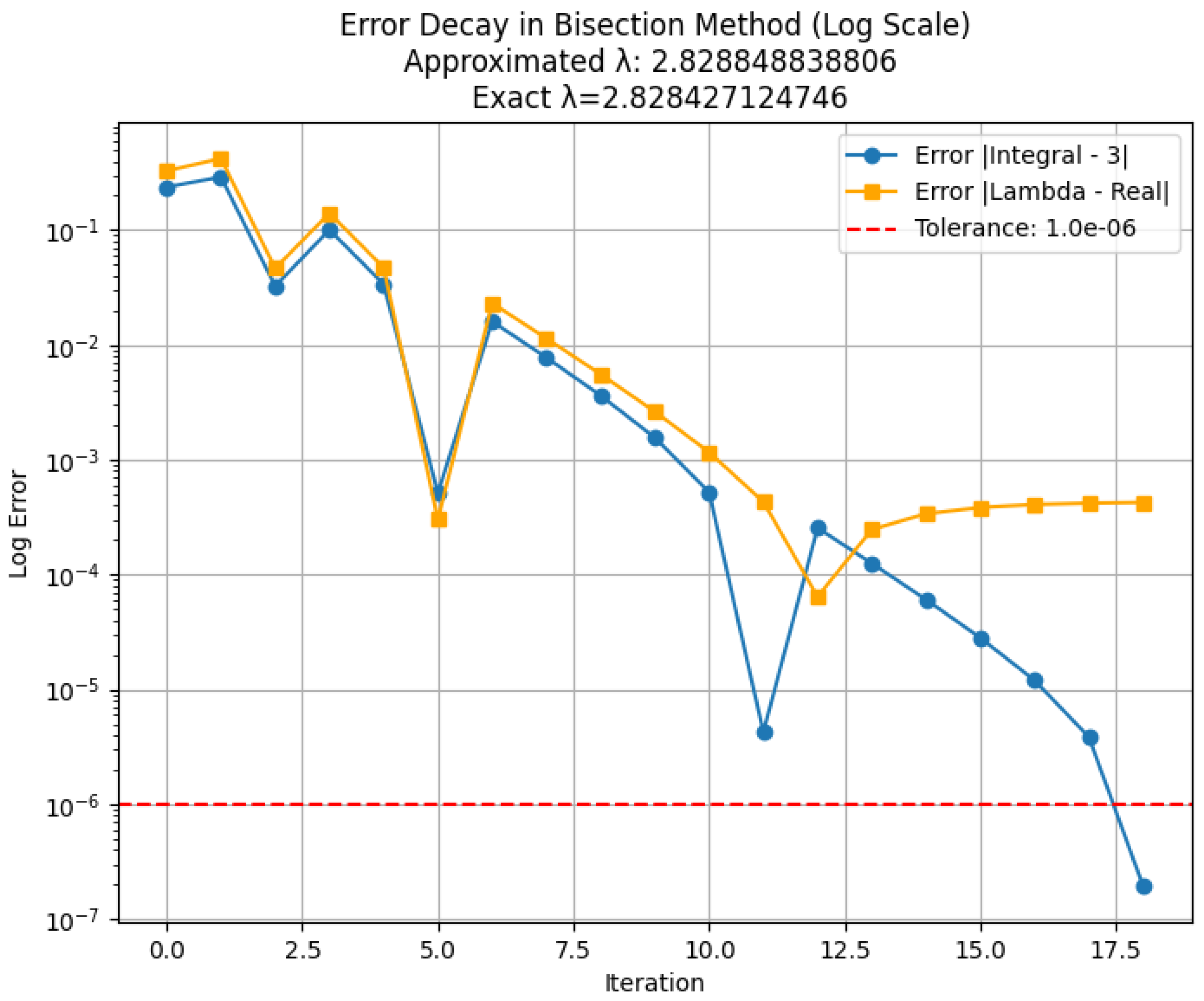
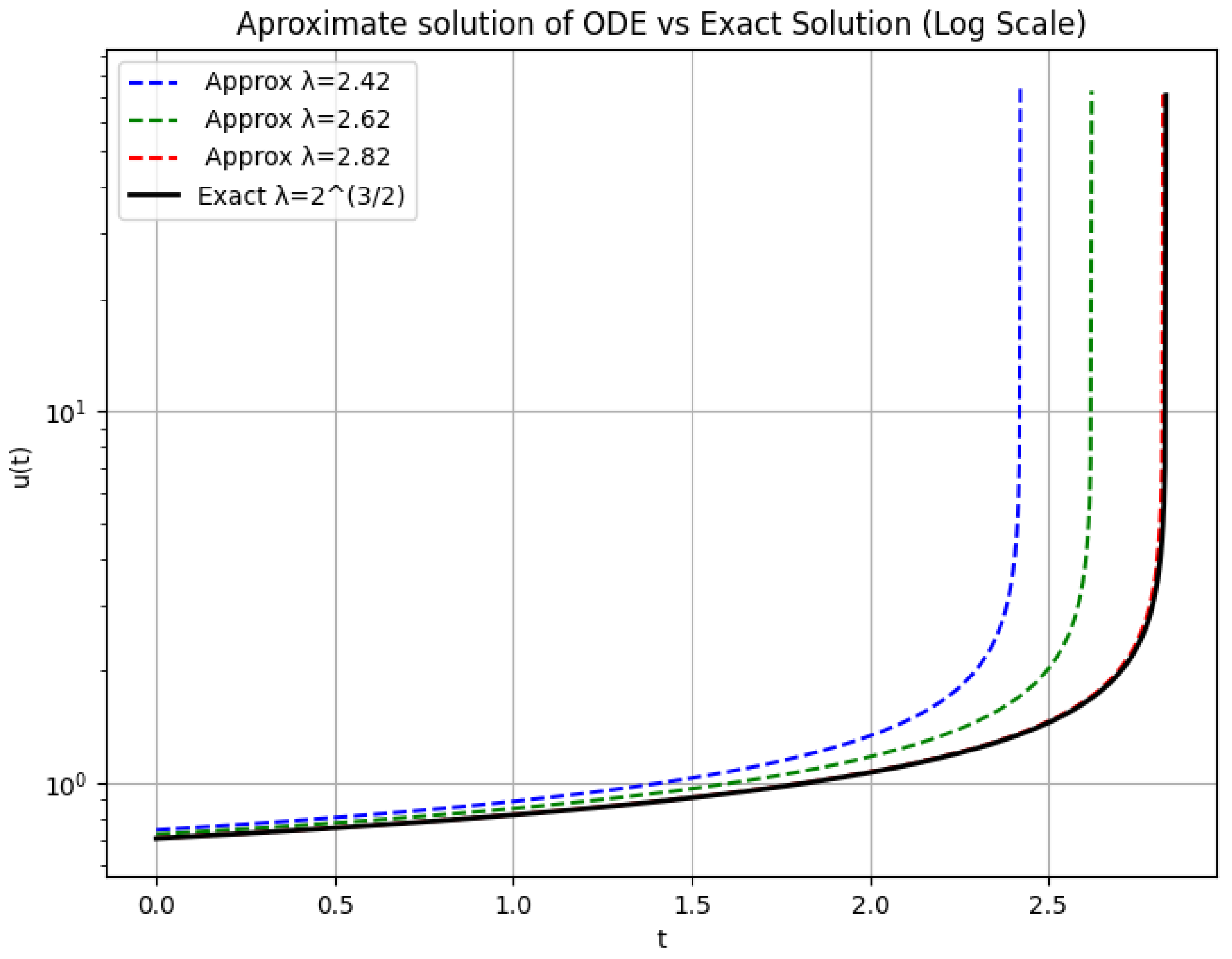
3. Approximate Solving of the Control Problem

Starting from the lower and upper solutions $\underline{\lambda },$ $\overline{\lambda },$ one can approximate ${\lambda }^{*}$ by using the following algorithm (Algorithm 1). For a similar use of this method, we refer the reader to [19].    

Algorithm 1: Bisection algorithm

Step 0 (initialization): $k:=0,{\underline{\lambda }}_0:=\underline{\lambda },$${\overline{\lambda }}_0:=$$\overline{\lambda }$. Step $k\left(k\ge 1\right):$ compute $\lambda :={\displaystyle \frac{{\underline{\lambda }}_{k-1}+{\overline{\lambda }}_{k-1}}{2}};$ If $\phi \left(\lambda \right)=p,$ then ${\lambda }^{*}=\lambda$ and we are finished; If $\phi \left(\lambda \right)<p,$ then set ${\underline{\lambda }}_k:=\lambda$ and ${\overline{\lambda }}_k:={\overline{\lambda }}_{k-1}$ and repeat Step k with $k:=k+1;$ If $\phi \left(\lambda \right)>p,$ then set ${\underline{\lambda }}_k:={\underline{\lambda }}_{k-1}$ and ${\overline{\lambda }}_k:=\lambda$ and repeat Step k with $k:=k+1;$ Stop criterion: if $\left|\phi \left(\lambda \right)-p\right|\le \epsilon ,$ then $\lambda \simeq {\lambda }^{*}$ (with error $\epsilon$).

We note that this step-by-step algorithm iteratively approximates the control solution. At each step, based on the obtained feedback, either the subsolution or the supersolution is improved.

Theorem 7.

Under assumptions (h1)–(h3), the bisection algorithm is convergent to a solution ${\lambda }^{*}$ of the control problem.

Proof. 

If the algorithm does not stop after a finite number of steps, then it generates two bounded and monotone (so convergent) sequences, $\left({\underline{\lambda }}_k\right)$ and $\left({\overline{\lambda }}_k\right),$ which in addition satisfy

$$\left|{\overline{\lambda }}_k-{\underline{\lambda }}_k\right|={\displaystyle \frac{\left|\overline{\lambda }-\underline{\lambda }\right|}{2^k}}\left(k\ge 0\right),$$

(21)

$$\phi \left({\underline{\lambda }}_k\right)<p,\phi \left({\overline{\lambda }}_k\right)>p.$$

(22)

From (21), the two sequences have the same limit denoted ${\lambda }^{*},$ while from (22), in virtue of the continuity Theorem 5, we obtain

$$\phi \left({\lambda }^{*}\right)\le p\mathrm{and}\phi \left({\lambda }^{*}\right)\ge p.$$

Hence, $\phi \left({\lambda }^{*}\right)=p$ as desired. □

Example 2.

A typical example of function f satisfying conditions (h1)–(h3) is

$$f(t,x,\lambda )={\displaystyle \frac{x}{a(\lambda -t)}},$$

(23)

where $a>1$. Clearly, $\theta \left(\lambda \right)=\lambda$. If in addition we take $u_0\left(\lambda \right)={\lambda }^{-{\displaystyle \frac{1}{a}}}$, we obtain the unique solution of problem (1),

$$u_{\lambda }\left(t\right)={\displaystyle \frac{1}{{(\lambda -t)}^{\frac{1}{a}}}}.$$

Therefore,

$$\phi \left(\lambda \right)={\int }_0^{\lambda }{u}_{\lambda }\left(s\right)ds={\displaystyle \frac{a}{a-1}}{\lambda }^{{\displaystyle \frac{a-1}{a}}},$$

which is well-defined and continuous on $(0,\infty )$.

We conclude this example with some numerical simulations for the function f defined in (23), with $a=3$. Our aim is to determine ${\lambda }^{*}$ such that $\phi \left({\lambda }^{*}\right)=3$. The exact value is known to be ${\lambda }_{\mathrm{exact}}=2^{{\displaystyle \frac{3}{2}}}$. For the lower and upper solutions of the control problem, we take $\underline{\lambda }=1$ and $\overline{\lambda }=4$, respectively, while the tolerance $\epsilon$ is chosen to be $\epsilon ={10}^{-6}$.

In Figure 1, the blue curve represents the error between $\phi \left(\lambda \right)$ and $p=3$, where $\lambda$ at each step k is $\lambda :={\displaystyle \frac{{\underline{\lambda }}_{k-1}+{\overline{\lambda }}_{k-1}}{2}},$ while the orange curve represents the difference between the calculated value of $\lambda$ and the exact value ${\lambda }_{\mathrm{exact}}$. After 18 iterations, the approximate value of the control is found to be

$${\lambda }^{*}=2.828848838806.$$

In Figure 2, the graph of $u_{\lambda }$ is plotted for the last three values of $\lambda$ obtained from the bisection algorithm (those corresponding to the lowest error in the previous figure). We see that, for $\lambda =2.82$, the graph of the function $u_{\lambda }$ almost overlaps with the graph of $u_{{\lambda }_{\mathrm{exact}}}$.

Remark 2.

The conclusion of Theorem 5 clearly remains valid under assumptions (h1)–(h3), if, instead of the functionals ${\psi }_{\lambda }$, we consider the functionals

$${\overline{\psi }}_{\lambda }\left(u\right)={\int }_0^{\theta \left(\lambda \right)}\left|u\left(s\right)\right|ds,$$

and instead of φ we correspondingly take

$$\tilde{\phi }\left(\lambda \right)={\int }_0^{\theta \left(\lambda \right)}\left|u_{\lambda }\left(s\right)\right|ds.$$

Moreover, we can extend this result to $L_p$ type functionals of the form

$${\overline{\psi }}_{\lambda }\left(u\right)={\left({\int }_0^{\theta \left(\lambda \right)}{\left|u\left(s\right)\right|}^{p}ds\right)}^{{\displaystyle \frac{1}{p}}},$$

where $1\le p<\infty$. In this case, if we replace (h3) by condition

(h3^′) 

, there exists a constant $a>p$ such that, for all $\lambda >0$, one has

$$\left|f(t,x,\lambda )\right|\le {\displaystyle \frac{\left|x\right|}{a\left(\theta \right(\lambda )-t)}}+C_{\lambda },$$

for all $t\in [0,\theta (\lambda \left)\right)$ and all $x\in \mathbb{R}$, where $C_{\lambda }\ge 0$ and the map $\lambda \mapsto C_{\lambda }$ is continuous.

4. Extension to Fractional Differential Equations

The above results can be generalized to fractional differential equations with moving singularities. Such problems more accurately describe various physical, biological, or medical processes (see, e.g., [20,21,22,23]). Therefore, our results related to problem (1) can be extended to the following problem:

$$\begin{array}{c}\hfill \left\{\begin{array}{c}{}^{c}D^{\alpha }u\left(t\right)=f(t,u\left(t\right),\lambda ),t\in [0,\theta \left(\lambda \right))\hfill \\ u\left(0\right)=u_0\left(\lambda \right),\hfill \end{array}\right.\end{array}$$

where ${}^{c}D^{\alpha }$ is the Caputo fractional derivative and $0<\alpha <1$. As shown in the literature, the above problem is equivalent to the Voltera integral equation:

$$u_{\lambda }\left(t\right)=u_0\left(\lambda \right)+{\displaystyle \frac{1}{\Gamma \left(\alpha \right)}}{\int }_0^t{(t-s)}^{\alpha -1}f(s,u\left(s\right),\lambda )ds.$$

Note that, in our case, the control problem remain unchanged, i.e., find $\lambda$ such that

$${\int }_0^{\theta \left(\lambda \right)}{u}_{\lambda }\left(s\right)ds=p.$$

Since our entire analysis is grounded in the integral form of the Cauchy problem, we can easily extend the proof steps to address this more general case. The flexibility of the integral formulation allows for the adaptation of our methods without significant modifications. By imposing conditions similar to those outlined in (h1) and (h2), we can rigorously establish the controllability of the problem.

5. Conclusions

The analyzed control problem in this paper is atypical in several aspects: (a) it refers to equations with singularity; (b) the singularity itself depends on the control variable; (c) the controllability condition involves the moving singularity. All these aspects make the analysis much more complex and adapted to the specifics of the problem. The working techniques can also be taken into account for the investigation of other types of singular equations and controllability conditions, including singular partial differential equations (see, e.g., [6]). We believe and anticipate that the ideas and techniques used in this article will have the high degree of suitability for the specifics of each individual problem in future research.

References

1. Torres, P.J. Mathematical Models with Singularities: A Zoo of Singular Creatures; Atlantis Press: Amsterdam, The Netherlands, 2015. [Google Scholar]
2. O’Regan, D. Theory of Singular Boundary Value Problems; World Scientific Publishing: River Edge, NJ, USA, 1994. [Google Scholar]
3. Callegari, A.; Nachman, A. A nonlinear singular boundary value problem in the theory of pseudoplasitc fluids. SIAM J. Appl. Math. 1980, 38, 275–282. [Google Scholar]
4. Gingold, H. Rosenblat, S. Differential equations with moving singularities. SIAM J. Math. Anal 1976, 7, 942–957. [Google Scholar]
5. Gingold, H. Introduction to differential equations with moving singularities. Rocky Mt. J. Math. 1976, 6, 571–574. [Google Scholar] [CrossRef]
6. Fila, M.; Takahashi, J.; Yanagida, E. Solutions with moving singularities for a one-dimensional nonlinear diffusion equation. Math. Ann. 2024, 390, 5383–5413. [Google Scholar] [CrossRef]
7. Nicolescu, M.; Dinculeanu, N.; Marcus, S. Manual de Analiză Matematicăa (II); Editura Didactică şi Pedagogică: Bucureşti, Romania, 1964. (In Romanian) [Google Scholar]
8. Haplea, I.Ş.; Parajdi, L.G.; Precup, R. On the controllability of a system modeling cell dynamics related to leukemia. Symmetry 2021, 13, 1867. [Google Scholar] [CrossRef]
9. Precup, R. On some applications of the controllability principle for fixed point equations. Results Appl. Math. 2022, 13, 100236. [Google Scholar] [CrossRef]
10. Coron, J.M. Control and Nonlinearity; AMS: Providence, RI, USA, 2007. [Google Scholar]
11. Coddington, E.A. An Introduction to Ordinary Differential Equations; Dover: New York, NY, USA, 1961. [Google Scholar]
12. Precup, R. Ordinary Differential Equations; De Gruyter: Berlin, Germany, 2018. [Google Scholar]
13. O’Regan, D.; Precup, R. Theorems of Leray-Schauder Type and Applications; CRC Press: Boca Raton, FL, USA, 2002. [Google Scholar]
14. Ciarlet, G. Linear and Nonlinear Functional Analysis with Applications; SIAM: Philadelphia, PA, USA, 2013. [Google Scholar]
15. Le Dret, H. Nonlinear Elliptic Partial Differential Equations; Springer: Berlin, Germany, 2018. [Google Scholar]
16. Gronwall, T.H. Note on the derivatives with respect to a parameter of the solutions of a system of differential equations. Ann. Math. 1919, 20, 292–296. [Google Scholar]
17. Pachpatte, B.G.; Ames, W.F. Inequalities for Differential and Integral Equations; Academic Press: Cambridge, MA, USA, 1997. [Google Scholar]
18. Rudin, W. Principles of Mathematical Analysis; MacGraw-Hill: New York, NY, USA, 1976. [Google Scholar]
19. Parajdi, L.G.; Precup, R.; Haplea, I.S. A method of lower and upper solutions for control problems and application to a model of bone marrow transplantation. Int. J. Appl. Math. Comput. Sci. 2023, 33, 409–418. [Google Scholar]
20. Samko, S.G.; Kilbas, A.A.; Marichev, O.I. Fractional Integrals and Derivatives: Theory and Applications; Gordon and Breach Science Publishers: Yverdon, Switzerland, 1993. [Google Scholar]
21. Kilbas, A.A.; Trujillo, J.J. Differentiale equations of fractional order: Methods, results and problems-I. Appl. Anal. 2001, 78, 153–192. [Google Scholar]
22. Benchohra, M.; Hamani, S.; Ntouyas, S.K. Boundary value problems for differential equations with fractional order and nonlocal conditions. Nonlinear Anal. 2009, 71, 2391–2396. [Google Scholar] [CrossRef]
23. Podlubny, I. Fractional Differential Equations; Mathematics in Sciences and Engineering; Academic Press: San Diego, CA, USA, 1999; Volume 198. [Google Scholar]
Figure 1. Error decay in the bisection method.
Fractalfract 09 00198 g001
Figure 2. Approximate solution u λ vs. exact solution u λ exact .
Fractalfract 09 00198 g002
Disclaimer/Publisher’s Note: The statements, opinions and data contained in all publications are solely those of the individual author(s) and contributor(s) and not of MDPI and/or the editor(s). MDPI and/or the editor(s) disclaim responsibility for any injury to people or property resulting from any ideas, methods, instructions or products referred to in the content.