Tempered Riemann–Liouville Fractional Operators: Stability Analysis and Their Role in Kinetic Equations

Abstract

Mathematics and physics are deeply interconnected. In fact, physics relies on mathematical tools like calculus and differential equations. The aim of this article is to introduce tempered Riemann–Liouville (RL) fractional operators and their properties with applications in mathematical physics. The tempered RL substantial fractional derivative is also defined, and its properties are discussed. The Laplace transforms (LTs) of the introduced fractional operators are evaluated. The Hyers–Ulam stability and the existence of a novel tempered fractional differential equation are examined. Moreover, a fractional integro-differential kinetic equation is formulated, and the LT is used to find its solution. A growth model and its graphical representation are established, highlighting the role of novel fractional operators in modeling complex dynamical systems. The developed mathematical framework offers valuable insights into solving a range of scenarios in mathematical physics.

1. Introduction

In many different scientific fields, fractional calculus is a helpful tool for explaining complicated phenomena. In simple terms, it is classical calculus extended to non-integer orders. Recent studies have shown that fractional calculus is used to represent a wide range of systems with different properties and long-term reliability. Developments in fractional operators like Riemann–Liouville and Gerasimov–Caputo by such works as [1,2] have made effective solutions of fractional differential equations possible. In order to address ever more complex problems in mathematical physics, this has motivated the development of more specialized operators.

The Tautochrone issue was solved by Abel [3], who is credited with spreading the use of fractional calculus. Furthermore, a variety of domains, including the theory of groups, electromagnetic theory [4], polymer compounds [5], fluid mechanics [6], quantum mechanics [7], wave theory [8], the study of biophysics [9], spectral analysis [10] and other fields, have employed the use of fractional calculus. Despite its long history, fractional calculus has attracted more attention in recent years due to the incredible outcomes it yields when applied to modeling real-world problems [11,12]. Since fractional calculus has multiple fractional operators, researchers can choose the one that best fits their particular modeling requirements, which is what makes it special.

Notable definitions of fractional operators include ones by Grünwald–Letnikov, Caputo, Riemann–Liouville and Hadamard [13,14]. These formulations, which use single kernel integrals, are commonly used in the study of memory effect issues [15]. Fractional derivatives are characterized by fractional calculus via the fractional integral [16]. Fractional operators come in many forms; however, tempered fractional operators have attracted significant interest due to their practical applications. These serve as an extension of fractional calculus and exhibit flexible behavior to solve more complex problems compared to existing operators. As far as we know, the initial formulations of fractional integration incorporating weak singular and exponential kernels were documented in Buschmann’s prior research [17]. For alternative definitions of tempered fractional integration, refer to the works found in books [16,18,19] and their associated references. The generalized tempered Riemann–Liouville fractional (RLF) calculus model has garnered growing attention in recent years due to its applications in stochastic and dynamical systems. Although prior research has focused mostly on numerical techniques and applications, there has been a relatively small amount of research focusing on pure analytical elements of this model. Our goal in this work is to perform a thorough analysis of the operators and rigorously establish several kinds of mathematical facts regarding them. These results are fundamental to developing the theoretical foundation of the tempered fractional calculus model.

This article is structured as follows: Section 2 presents the essential context with definitions of the fractional differential and integral operators mentioned above and statements of a few fundamental facts concerning them. In Section 3, we introduce the new form of the tempered fractional integral and discuss its boundedeness and fundamental properties. In Section 4, we present the corresponding derivative of the newly defined fractional operator and its properties, such as the inverse property. In Section 5, we evaluate the LT of newly introduced operators. In Section 6, we develop a new form of the tempered fractional differential equation and establish its uniqueness, existence and Hyers–Ulam stability criteria. In Section 7, we focus on examining the new generalized fractional kinetic integro-differential equation and we establish its solution. In Section 8, we summaries our primary findings and possible directions for further study in this field.

2. Preliminaries

In this section, we provide a brief summary of significant preliminary work before beginning our new investigation. Diaz et al. [20] outlined the definitions for the $\mathbf{k}$-gamma and $\mathbf{k}$-beta functions as follows:

Definition 1.

The $\mathbf{k}$-gamma function, which extends the traditional Γ function, is described as follows:

$${\Gamma }_{\mathbf{k}}\left(\varrho \right)=\underset{n\to \infty }{lim}{\displaystyle \frac{n!{\mathbf{k}}^n{\left(n\mathbf{k}\right)}^{\frac{\varrho }{\mathbf{k}}-1}}{{\left(\varrho \right)}_{n,\mathbf{k}}}},\mathbf{k}>0,\mathbf{R}\left(\varrho \right)>0,$$

where ${\left(\varrho \right)}_{n,\mathbf{k}}=\varrho (\varrho +\mathbf{k})(\varrho +2\mathbf{k})...(\varrho +(n-1)\mathbf{k}),n\ge 1$ is referred the Pochhammer $\mathbf{k}$ symbol. Another representation can be stated as

$${\Gamma }_{\mathbf{k}}\left(\varrho \right)=\underset{0}{\overset{\infty }{\int }}{\vartheta }^{\varrho -1}{e}^{{\displaystyle \frac{-{\vartheta }^{\mathbf{k}}}{\mathbf{k}}}}d\vartheta ,\mathbf{R}\left(\varrho \right)>0.$$

Obviously, $\Gamma \left(\varrho \right)={lim}_{\mathbf{k}\to 1}{\Gamma }_{\mathbf{k}}\left(\varrho \right)$ and ${\Gamma }_{\mathbf{k}}\left(\varrho \right)={\mathbf{k}}^{{\displaystyle \frac{\varrho }{\mathbf{k}}}-1}\Gamma \left({\displaystyle \frac{\varrho }{\mathbf{k}}}\right)$.

Definition 2.

The $\mathbf{k}$-beta function can be stated by the following relations for $\Re \left(\varrho \right),\Re \left(\beta \right)>0$ and $\mathbf{k}>0$:

$$B_{\mathbf{k}}(\varrho ,\beta )={\displaystyle \frac{1}{\mathbf{k}}}{\int }_0^1{\tau }^{{\displaystyle \frac{\varrho }{\mathbf{k}}}-1}{(1-\tau )}^{{\displaystyle \frac{\beta }{\mathbf{k}}}-1}d\tau .$$

The identity $B_{\mathbf{k}}(\varrho ,\beta )={\displaystyle \frac{{\Gamma }_{\mathbf{k}}\left(\varrho \right){\Gamma }_{\mathbf{k}}\left(\beta \right)}{{\Gamma }_{\mathbf{k}}(\varrho +\beta )}}$ describes the relation between the functions ${\Gamma }_{\mathbf{k}}$ and $B_{\mathbf{k}}$.

The following definition defines the RLF integrals presented in [11]:

Definition 3.

Let Φ∈$L_1[\sigma ,\delta ]$. Then, RLF integrals of order $\varrho >0$ are defined by

$$({\mathcal{I}}_{{\sigma }^{+}}^{\varrho }\Phi )\left(\vartheta \right)={\displaystyle \frac{1}{\Gamma \left(\varrho \right)}}{\int }_{\sigma }^{\vartheta }{(\vartheta -\zeta )}^{\varrho -1}\Phi \left(\zeta \right)d\zeta ,\vartheta >\sigma ,$$

and

$$({\mathcal{I}}_{{\delta }^{-}}^{\varrho }\Phi )\left(\vartheta \right)={\displaystyle \frac{1}{\Gamma \left(\varrho \right)}}{\int }_{\vartheta }^{\delta }{(\zeta -\vartheta )}^{\varrho -1}\Phi \left(\zeta \right)d\zeta ,\vartheta <\delta .$$

If we set $\varrho =1$, the RLF integral becomes equivalent to the classical integral. An overview of the fundamental descriptions and modified structures of the tempered Riemann–Liouville fractional (TRLF) integral operators, as presented in [21,22] is currently being conducted and is given by the following definition:

Definition 4.

Let Φ∈$L_1[\sigma ,\delta ]$. Then, TRLF integral operators of order $\varrho >0$ are defined by

$$({\mathcal{I}}_{{\sigma }^{+}}^{(\varrho ,\lambda )}\Phi )\left(\vartheta \right)={\displaystyle \frac{1}{\Gamma \left(\varrho \right)}}{\int }_{\sigma }^{\vartheta }{(\vartheta -\zeta )}^{\varrho -1}{e}^{-\lambda (\vartheta -\zeta )}\Phi \left(\zeta \right)d\zeta ,\vartheta \in [\sigma ,\delta ],$$

and

$$({\mathcal{I}}_{{\delta }^{-}}^{(\varrho ,\lambda )}\Phi )\left(\vartheta \right)={\displaystyle \frac{1}{\Gamma \left(\varrho \right)}}{\int }_{\vartheta }^{\delta }{(\zeta -\vartheta )}^{\varrho -1}{e}^{-\lambda (\zeta -\vartheta )}\Phi \left(\zeta \right)d\zeta ,\vartheta \in [\sigma ,\delta ].$$

Definition 5.

([23,24]). Suppose that Φ is a function that is continuous on $[0,\infty )$. When $n-1<\varrho <n$, $\lambda \ge 0$, and n is a positive integer, the TRLF derivative is defined as follows:

$$\begin{array}{cc}\hfill ({\mathcal{D}}_{a^{+}}^{(\varrho ,\lambda )}\Phi )\left(\vartheta \right)=& e^{-\lambda \vartheta }{\mathcal{D}}_{a^{+}}^{\varrho }(e^{\lambda \vartheta }\Phi )\left(\vartheta \right)\hfill \\ \hfill & ={\displaystyle \frac{e^{-\lambda \vartheta }}{\Gamma (n-\varrho )}}{\displaystyle \frac{d^n}{{d\vartheta }^n}}{\int }_a^{\vartheta }{(\vartheta -\zeta )}^{n-\varrho -1}{e}^{\lambda \zeta }\Phi \left(\zeta \right)d\zeta ,\forall 0<\zeta <\vartheta <\infty ,\hfill \end{array}$$

where $n=\left[\varrho \right]+1$, and ${\mathcal{D}}_{a^{+}}^{\varrho }(e^{\lambda \vartheta }\Phi )\left(\vartheta \right)$ denotes the RLF derivative [25].

Fahad et al. [26] introduced the generalized LT, which is defined as follows:

Definition 6.

Given real-valued functions Φ and ℧ defined on the interval $[a,\infty )$, where $\mho \left(\vartheta \right)$ is continuous and ${\mho }^{\prime }\left(\vartheta \right)>0$ for all ϑ in the interval $[a,\infty )$, the generalized LT of Φ can be expressed as

$$L_{\mho }\{\Phi \left(\zeta \right)\}\left(u\right)={\int }_a^{\infty }{e}^{-u(\mho (\zeta )-\mho (a\left)\right)}\Phi \left(\zeta \right){\mho }^{\prime }\left(\zeta \right)d\zeta ,$$

which holds for every value of u.

Theorem 1.

([26]). Let $\Phi \in AC[a,\vartheta )$ have the ℧-exponential order. The generalized LT of $\mathcal{D}\Phi$ exists if $\mathcal{D}\Phi$ is a piecewise continuous function on each interval $[a,T]$ and

$${\mathbf{L}}_{\mho }\{\mathcal{D}\Phi \}\left(u\right)=u{\mathbf{L}}_{\mho }\{\Phi \left(\vartheta \right)\}\left(u\right)-\Phi \left(a\right).$$

Theorem 1 can be generalized as follows:

Theorem 2.

Let Φ be in the class $A{C}^{n-1}[a,\vartheta )$, such that ${\mathcal{D}}^{\mathbf{l}},\Phi$ for $\mathbf{l}=0,1,2,\dots ,n-1$ is of the ℧-exponential order. If ${\mathcal{D}}^n\Phi$ is a piecewise continuous function on each interval $[a,T]$, then the generalized LT of ${\mathcal{D}}^n\Phi$ exists and

$${\mathbf{L}}_{\mho }\{{\mathcal{D}}^n\Phi \}\left(u\right)=u^n{\mathbf{L}}_{\mho }\{\Phi \left(\vartheta \right)\}\left(u\right)-\sum _{\mathbf{l}=0}^{n-1}{u}^{n-\mathbf{l}-1}{\Phi }_{\mathbf{l}}\left(a\right).$$

Definition 7.

([26]). The specification of the convolution of Φ and ℧ functions is given by

$$\begin{array}{cc}\hfill (\Phi {\ast }_{\mho }h)\left(\vartheta \right)=& {\int }_a^{\vartheta }\left({\mho }^{-1}(\mho \left(\vartheta \right)+\mho \left(a\right)-\mho \left(\zeta \right))\right)\hfill \\ \hfill & \times \Phi \left({\mho }^{-1}(\mho \left(\vartheta \right)+\mho \left(a\right)-\mho \left(\zeta \right))\right)h\left(\zeta \right){\mho }^{\prime }\left(\zeta \right)d\zeta .\hfill \end{array}$$

3. A New Form of a Tempered Riemann–Liouville Fractional Integral

In this section, we define a new form of the TRLF integral and examine its boundedness and certain characteristics.

Definition 8.

Let Φ be a function that is continuous on the finite real interval $[a,b]$. Then, the extended TRLF integral of order ϱ is defined by

$$({}_{\mathbf{k}}\mathcal{I}_{a^{+}}^{(\varrho ,\lambda )}\Phi )\left(\vartheta \right)={\displaystyle \frac{1}{\mathbf{k}{\Gamma }_{\mathbf{k}}\left(\varrho \right)}}{\int }_a^{\vartheta }{(\vartheta -\zeta )}^{{\displaystyle \frac{\varrho }{\mathbf{k}}}-1}{e}^{-\lambda (\vartheta -\zeta )}\Phi \left(\zeta \right)d\zeta ,\vartheta \in [a,b],$$

(1)

where $\varrho ,\mathbf{k}>0$ and $\lambda \ge 0$.

Remark 1.

It is important to highlight that this integral operator includes numerous fractional integral operators. By setting $\mathbf{k}=1$, we obtain the TRLF integral [21,22]. By choosing $\lambda =0$, the $\mathbf{k}$-RLF integral is obtained [27]. The choice of parameters $\mathbf{k}=1$ and $\lambda =0$ allows us to obtain the RLF integral [11].

Next, we introduce the space in which the new form of TRLF integrals is bounded.

Definition 9.

Let a function Φ be defined on the interval $[a,b]$ and $X^p(a,b)$, with $1\le p\le \infty$ being a space of Lebesgue measurable functions. Then, we have ${\Vert \Phi \Vert }_{X^p}<\infty$, such that

$${\Vert \Phi \Vert }_{X^p}=[{\int }_a^b\mid \Phi \left(\vartheta \right)e^{-\lambda \vartheta }{\mid }^{p}d\vartheta {]}^{{\displaystyle \frac{1}{p}}},1\le p<\infty ,$$

$\lambda \ge 0$ and

$${\Vert \Phi \Vert }_{X^{\infty }}=esssu{p}_{a\le \vartheta \le b}|\Phi \left(\vartheta \right)|<\infty .$$

Note that $\Phi \in X^p(a,b)$⇔$e^{-\lambda \vartheta }\Phi \left(\vartheta \right)\in L_p(a,b)$ for $1\le p<\infty$ and $\Phi \in X_{\mho }^{\infty }(a,b)$⇔$e^{-\lambda \vartheta }\Phi \left(\vartheta \right)\in L_{\infty }(a,b)$.

Theorem 3.

Let $\varrho >0$, $\mathbf{k}>0$, $\lambda \ge 0$, $1\le p\le \infty$ and $\Phi \in X^p(a,b)$. Then, ${}_{\mathbf{k}}\mathcal{I}_{a^{+}}^{(\varrho ,\lambda )}\Phi$ is bounded in $X^p(a,b)$, i.e.,

$$\Vert {}_{\mathbf{k}}\mathcal{I}_{a^{+}}^{(\varrho ,\lambda )}\Phi \Vert X^p\le {\displaystyle \frac{{(b-a)}^{\frac{\varrho }{\mathbf{k}}}}{{\Gamma }_{\mathbf{k}}(\varrho +1)}}{\Vert \Phi \Vert }_{X^p}.$$

Proof. 

Assuming $1\le p<\infty$, we obtain

$$\begin{array}{cc}\hfill & \Vert {}_{\mathbf{k}}\mathcal{I}_{a^{+}}^{(\varrho ,\lambda )}\Phi \Vert X^p\hfill \\ \hfill & =\left[{\int }_a^b\right|{\displaystyle \frac{1}{\mathbf{k}{\Gamma }_{\mathbf{k}}\left(\varrho \right)}}{\int }_a^{\vartheta }{(\vartheta -\zeta )}^{{\displaystyle \frac{\varrho }{\mathbf{k}}}-1}{e}^{-\lambda (\vartheta -\zeta )}{e}^{-\lambda \zeta }\Phi \left(\zeta \right)d\zeta {|}^{p}d\vartheta {]}^{{\displaystyle \frac{1}{p}}}\hfill \\ \hfill & ={\displaystyle \frac{1}{\mathbf{k}{\Gamma }_{\mathbf{k}}\left(\varrho \right)}}\left[{\int }_a^b\right|{\int }_a^{\vartheta }{(\vartheta -\zeta )}^{{\displaystyle \frac{\varrho }{\mathbf{k}}}-1}{e}^{-\lambda \vartheta }\Phi \left(\zeta \right)d\zeta {|}^{p}d\vartheta {]}^{{\displaystyle \frac{1}{p}}}.\hfill \end{array}$$

(2)

By substituting $\vartheta =v$ and $\zeta =u$ on the right side of (2), we have

$$\begin{array}{cc}\hfill & {\Vert }_{\mathbf{k}}{\mathcal{I}}_{a^{+}}^{\varrho }{\Phi \Vert }_{X^p}\hfill \\ \hfill & ={\displaystyle \frac{1}{\mathbf{k}{\Gamma }_{\mathbf{k}}\left(\varrho \right)}}[{\int }_a^b|{\int }_a^{\vartheta }{(v-u)}^{{\displaystyle \frac{\varrho }{\mathbf{k}}}-1}{e}^{-\lambda v}\Phi \left(u\right)du{|}^{p}dv{]}^{{\displaystyle \frac{1}{p}}}.\hfill \end{array}$$

By utilizing Minkowski’s inequality, we have

$$\begin{array}{cc}\hfill & \Vert {}_{\mathbf{k}}\mathcal{I}_{a^{+}}^{\varrho }\Phi \Vert X^p\hfill \\ \hfill & \le {\displaystyle \frac{1}{\mathbf{k}{\Gamma }_{\mathbf{k}}\left(\varrho \right)}}{\int }_a^b|\Phi \left(u\right)e^{-\lambda u}|{\left[{\int }_u^b{(v-u)}^{({\displaystyle \frac{\varrho }{\mathbf{k}}}-1)p}dv\right]}^{{\displaystyle \frac{1}{p}}}du\hfill \\ \hfill & \le {\displaystyle \frac{1}{\mathbf{k}{\Gamma }_{\mathbf{k}}\left(\varrho \right)}}{\int }_a^b|\Phi \left(u\right)|{\left[{\displaystyle \frac{{(b-u)}^{(\frac{\varrho }{\mathbf{k}}-1)p+1}}{(\frac{\varrho }{\mathbf{k}}-1)p+1}}\right]}^{{\displaystyle \frac{1}{p}}}du.\hfill \end{array}$$

By applying Hölder’s inequality, we obtain

$$\begin{array}{cc}\hfill \Vert {}_{\mathbf{k}}\mathcal{I}_{a^{+}}^{(\varrho ,\lambda )}\Phi \Vert X^p& \le {\displaystyle \frac{1}{\mathbf{k}{\Gamma }_{\mathbf{k}}\left(\varrho \right)}}{\left[{\int }_a^b{|\Phi \left(u\right)e^{-\lambda u}|}^{p}du\right]}^{{\displaystyle \frac{1}{p}}}\hfill \\ \hfill & \times {\left[{\int }_a^b{\left({\displaystyle \frac{{(b-u)}^{(\frac{\varrho }{\mathbf{k}}-1)p+1}}{(\frac{\varrho }{\mathbf{k}}-1)p+1}}\right)}^{{\displaystyle \frac{q}{p}}}du\right]}^{{\displaystyle \frac{1}{q}}},\hfill \end{array}$$

where ${\displaystyle \frac{1}{p}}+{\displaystyle \frac{1}{q}}=1$.

$$\begin{array}{cc}\hfill {\Vert {}_{\mathbf{k}}\mathcal{I}_{a^{+}}^{\varrho }\Phi \Vert }_{X^p}& \le {\displaystyle \frac{1}{\mathbf{k}{\Gamma }_{\mathbf{k}}\left(\varrho \right)}}{\left[{\int }_a^b{|\Phi \left(\zeta \right)e^{-\lambda \zeta }|}^{p}d\zeta \right]}^{{\displaystyle \frac{1}{p}}}{\left[{\int }_a^b{\left({\displaystyle \frac{{(b-u)}^{(\frac{\varrho }{\mathbf{k}}-1)p+1}}{(\frac{\varrho }{\mathbf{k}}-1)p+1}}\right)}^{{\displaystyle \frac{q}{p}}}du\right]}^{{\displaystyle \frac{1}{q}}}\hfill \\ \hfill & \le {\displaystyle \frac{{(b-a)}^{\frac{\varrho }{\mathbf{k}}}}{{\Gamma }_{\mathbf{k}}(\varrho +1)}}{\Vert \Phi \Vert }_{X^p}.\hfill \end{array}$$

For $p=\infty$, we obtain

$$\begin{array}{c}\hfill \left|({}_{\mathbf{k}}\mathcal{I}_{a^{+}}^{\varrho }\Phi (\vartheta )\right|={\displaystyle \frac{{(b-a)}^{\frac{\varrho }{\mathbf{k}}}}{{\Gamma }_{\mathbf{k}}(\varrho +1)}}{\Vert \Phi \Vert }_{X^{\infty }}.\end{array}$$

This completes the proof of the result. □

Theorem 4.

Suppose Φ to be a function that is continuous on $[a,b]$ and $\mathbf{k}>0$, $\lambda \ge 0$, which allows us to obtain the following:

$${}_{\mathbf{k}}\mathcal{I}_{a^{+}}^{(\beta ,\lambda )}\Phi [{}_{\mathbf{k}}\mathcal{I}_{a^{+}}^{(\varrho ,\lambda )}\Phi \left(\vartheta \right)]={}_{\mathbf{k}}\mathcal{I}_{a^{+}}^{(\varrho ,\lambda )}[{}_{\mathbf{k}}\mathcal{I}_{a^{+}}^{(\beta ,\lambda )}\Phi \left(\vartheta \right)]={}_{\mathbf{k}}\mathcal{I}_{a^{+}}^{(\varrho +\beta ,\lambda )}\Phi \left(\vartheta \right),$$

for all $\varrho ,\beta >0$ and $\vartheta \in [a,b]$.

Proof. 

By utilizing Definition 8 and Dirichlet’s formula, we obtain

$$\begin{array}{cc}\hfill & {}_{\mathbf{k}}\mathcal{I}_{a^{+}}^{(\varrho ,\lambda )}[{}_{\mathbf{k}}\mathcal{I}_{a^{+}}^{(\beta ,\lambda )}\Phi \left(\vartheta \right)]\hfill \\ \hfill & ={\displaystyle \frac{1}{\mathbf{k}{\Gamma }_{\mathbf{k}}\left(\varrho \right)}}{\int }_a^{\vartheta }{(\vartheta -\zeta )}^{{\displaystyle \frac{\varrho }{\mathbf{k}}}-1}{e}^{-\lambda (\vartheta -\zeta )}({}_{\mathbf{k}}\mathcal{I}_{a^{+}}^{(\beta ,\lambda )}\Phi \left(\zeta \right))d\zeta \hfill \\ \hfill & ={\displaystyle \frac{e^{-\lambda \vartheta }}{\mathbf{k}{\Gamma }_{\mathbf{k}}\left(\varrho \right)}}{\int }_a^{\vartheta }{(\vartheta -\zeta )}^{{\displaystyle \frac{\varrho }{\mathbf{k}}}-1}{e}^{\lambda \zeta }\left[{\displaystyle \frac{1}{\mathbf{k}{\Gamma }_{\mathbf{k}}\left(\beta \right)}}{\int }_a^{\zeta }{(\zeta -\tau )}^{{\displaystyle \frac{\beta }{\mathbf{k}}}-1}{e}^{-\lambda (\zeta -\tau )}\Phi \left(\tau \right)d\tau \right]d\zeta \hfill \\ \hfill & ={\displaystyle \frac{e^{-\lambda \vartheta }}{{\mathbf{k}}^2{\Gamma }_{\mathbf{k}}\left(\varrho \right){\Gamma }_{\mathbf{k}}\left(\beta \right)}}{\int }_a^{\vartheta }{e}^{\lambda \tau }\Phi \left(\tau \right)\left[{\int }_{\tau }^{\vartheta }{(\vartheta -\zeta )}^{{\displaystyle \frac{\varrho }{\mathbf{k}}}-1}{(\zeta -\tau )}^{{\displaystyle \frac{\beta }{\mathbf{k}}}-1}dt\right]d\tau .\hfill \end{array}$$

(3)

By substituting $y={\displaystyle \frac{\zeta -\tau }{\vartheta -\tau }}$ on the right side of (3), we obtain

$$\begin{array}{cc}\hfill & {}_{\mathbf{k}}\mathcal{I}_{a^{+}}^{(\varrho ,\lambda )}[{}_{\mathbf{k}}\mathcal{I}_{a^{+}}^{(\beta ,\lambda )}\Phi \left(\vartheta \right)]\hfill \\ \hfill & ={\displaystyle \frac{e^{-\lambda \vartheta }}{{\mathbf{k}}^2{\Gamma }_{\mathbf{k}}\left(\varrho \right){\Gamma }_{\mathbf{k}}\left(\beta \right)}}{\int }_a^{\vartheta }{(\vartheta -\tau )}^{{\displaystyle \frac{\varrho +\beta }{\mathbf{k}}}-1}\mathbf{k}{B}_{\mathbf{k}}(\varrho ,\beta )e^{\lambda \tau }\Phi \left(\tau \right)d\tau \hfill \\ \hfill & ={\displaystyle \frac{1}{\mathbf{k}{\Gamma }_{\mathbf{k}}(\varrho +\beta )}}{\int }_a^{\vartheta }{(\vartheta -\tau )}^{{\displaystyle \frac{\varrho +\beta }{\mathbf{k}}}-1}{e}^{-\lambda (\vartheta -\tau )}\Phi \left(\tau \right)d\tau \hfill \\ \hfill & ={}_{\mathbf{k}}\mathcal{I}_{a^{+}}^{(\varrho +\beta ,\lambda )}\Phi \left(\vartheta \right).\hfill \end{array}$$

The proof is completed. □

Theorem 5.

Suppose ϱ, β, $\mathbf{k}>0$ and $\lambda \ge 0$. Then, we have

$${}_{\mathbf{k}}\mathcal{I}_{a^{+}}^{(\varrho ,\lambda )}\left[e^{-\lambda \zeta }{(\zeta -a)}^{{\displaystyle \frac{\beta }{\mathbf{k}}}-1}\right]={\displaystyle \frac{{\Gamma }_{\mathbf{k}}\left(\beta \right)e^{-\lambda \zeta }{(\zeta -a)}^{\frac{\varrho +\beta }{\mathbf{k}}-1}}{{\Gamma }_{\mathbf{k}}(\varrho +\beta )}}.$$

(4)

Proof. 

By utilizing Definition 8, we obtain

$$\begin{array}{cc}\hfill & {}_{\mathbf{k}}\mathcal{I}_{a^{+}}^{(\varrho ,\lambda )}\left[e^{-\lambda \zeta }{(\zeta -a)}^{{\displaystyle \frac{\beta }{\mathbf{k}}}-1}\right]\hfill \\ \hfill & ={\displaystyle \frac{1}{\mathbf{k}{\Gamma }_{\mathbf{k}}\left(\varrho \right)}}{\int }_a^{\vartheta }{(\vartheta -\zeta )}^{{\displaystyle \frac{\varrho }{\mathbf{k}}}-1}{e}^{-\lambda (\vartheta -\zeta )}{e}^{-\lambda \zeta }{(\zeta -a)}^{{\displaystyle \frac{\beta }{\mathbf{k}}}-1}d\zeta \hfill \\ \hfill & ={\displaystyle \frac{1}{\mathbf{k}{\Gamma }_{\mathbf{k}}\left(\varrho \right)}}{\int }_a^{\vartheta }{(\vartheta -\zeta )}^{{\displaystyle \frac{\varrho }{\mathbf{k}}}-1}{e}^{-\lambda \vartheta }{(\zeta -a)}^{{\displaystyle \frac{\beta }{\mathbf{k}}}-1}d\zeta .\hfill \end{array}$$

(5)

By substituting $y={\displaystyle \frac{\zeta -a}{\vartheta -a}}$ on the right side of (5), we obtain

$$\begin{array}{cc}\hfill & {}_{\mathbf{k}}\mathcal{I}_{a^{+}}^{(\varrho ,\lambda )}\left[e^{\lambda \zeta }{(\zeta -a)}^{{\displaystyle \frac{\beta }{\mathbf{k}}}-1}\right]\hfill \\ \hfill & ={\displaystyle \frac{e^{-\lambda \vartheta }{(\vartheta -a)}^{\frac{\varrho +\beta }{\mathbf{k}}-1}}{\mathbf{k}{\Gamma }_{\mathbf{k}}\left(\varrho \right)}}{\int }_0^1{(1-y)}^{{\displaystyle \frac{\varrho }{\mathbf{k}}}-1}{\left(y\right)}^{{\displaystyle \frac{\beta }{\mathbf{k}}}-1}dy\hfill \\ \hfill & ={\displaystyle \frac{e^{-\lambda \vartheta }{(\vartheta -a)}^{\frac{\varrho +\beta }{\mathbf{k}}-1}}{\mathbf{k}{\Gamma }_{\mathbf{k}}\left(\varrho \right)}}\mathbf{k}{B}_{\mathbf{k}}(\varrho ,\beta )\hfill \\ \hfill & ={\displaystyle \frac{{\Gamma }_{\mathbf{k}}\left(\beta \right)e^{-\lambda \zeta }{(\zeta -a)}^{\frac{\varrho +\beta }{\mathbf{k}}-1}}{{\Gamma }_{\mathbf{k}}(\varrho +\beta )}}.\hfill \end{array}$$

The proof is completed. □

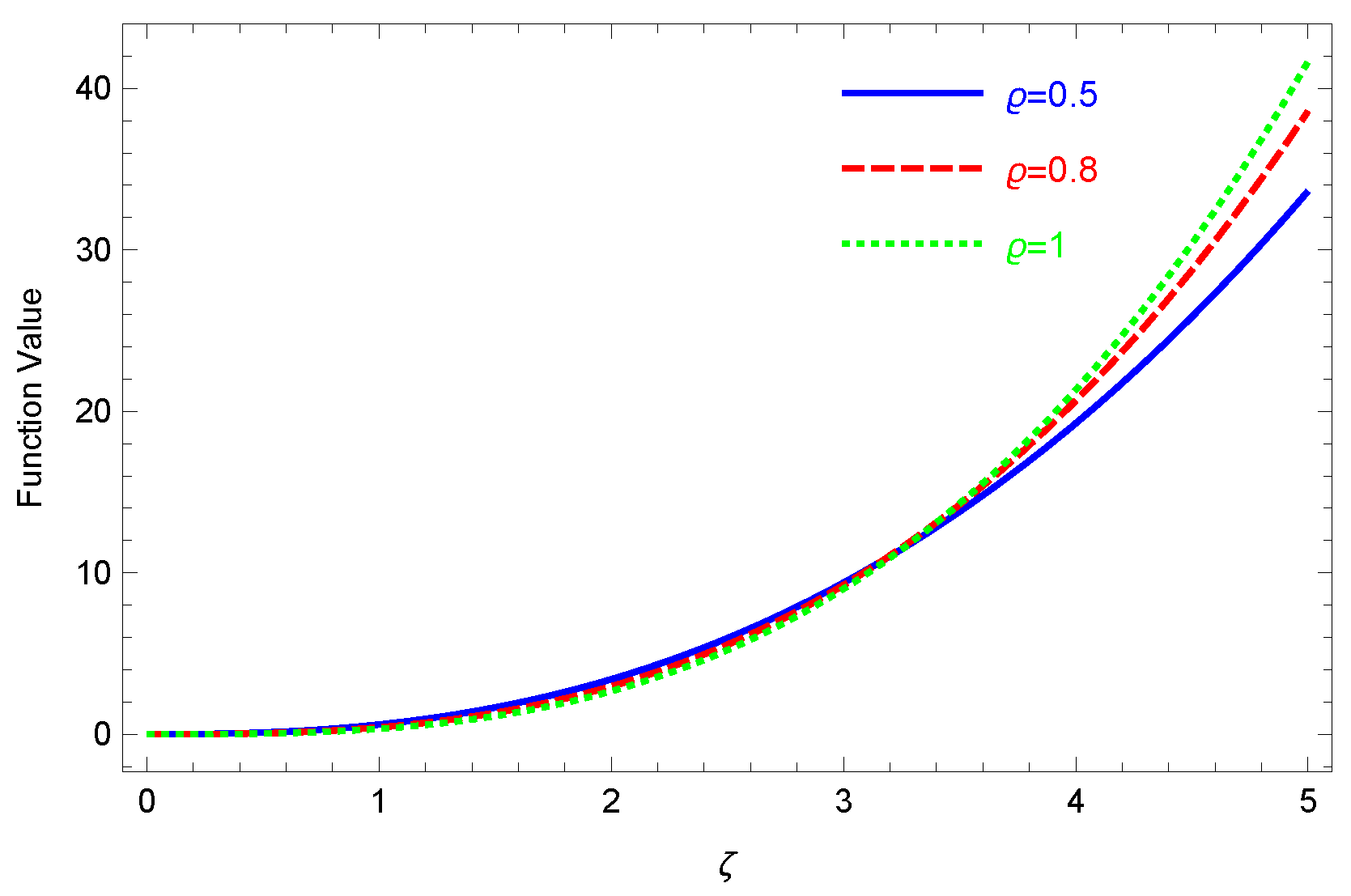
Example 1.

Based on selecting the parameters $\mathbf{k}=1$, $a=0$, $\beta =3$ and $\lambda =0$ in (4), distinct graphs emerge with various order selections are presented in Figure 1.

4. A New Form of a Tempered Riemann–Liouville Fractional Derivative

In this section, we present a new form of the TRLF derivative and investigate its fundamental properties.

Definition 10.

Consider Φ to be a function that is continuous on $[0,\infty )$ and $n-1<\varrho <n$, $n\in {\mathrm{N}}^{+}$, $\lambda \ge 0$. Then, for all $0<\zeta <\vartheta <\infty$, we have

$$\begin{array}{cc}\hfill ({}_{\mathbf{k}}\mathcal{D}_{a^{+}}^{(\varrho ,\lambda )}\Phi )\left(\vartheta \right)=& e^{-\lambda \vartheta }{}_{\mathbf{k}}\mathcal{D}_{a^{+}}^{\varrho }(e^{-\lambda \vartheta }\Phi )\left(\vartheta \right)={\displaystyle \frac{{\mathbf{k}}^{n-1}{e}^{\lambda \vartheta }}{{\Gamma }_{\mathbf{k}}(n\mathbf{k}-\varrho )}}{\displaystyle \frac{d^n}{d{\zeta }^n}}{\int }_a^{\vartheta }{(\vartheta -\zeta )}^{{\displaystyle \frac{n\mathbf{k}-\varrho }{\mathbf{k}}}-1}{e}^{\lambda \zeta }\Phi \left(\zeta \right)d\zeta ,\hfill \end{array}$$

where $n=\left[\varrho \right]+1$ and $\varrho ,\mathbf{k}>0$, which is called the new form of the TRLF derivative, provided that it exists.

Remark 2.

Notably, numerous derivative operators can be interpreted as specific cases of Operator (10). TRLF Derivative [23,24] is obtained for $\mathbf{k}=1$. By choosing $\lambda =0$, we obtain $\mathbf{k}$-RLF Derivative [28]. Moreover, RLF Derivative [29] is obtained by choosing $\mathbf{k}=1$ and $\lambda =0$.

The novel fractional derivative is defined as a substantial derivative [30,31].

Definition 11.

Let Φ be a function that is continuous on the interval $[0,\infty )$ and for $n-1<\varrho <n$, $n\in {\mathrm{N}}^{+}$, $\lambda \ge 0$. Then, the new form of the TRLF substantial derivative is defined as

$$\begin{array}{c}\hfill ({}_{\mathbf{k}}\mathcal{D}_{a^{+}}^{(\varrho ,\lambda )}\Phi )\left(\vartheta \right)=[\mathbf{k}({\displaystyle \frac{d}{d\vartheta }}+\lambda ){]}^n({}_{\mathbf{k}}\mathcal{I}_{a^{+}}^{(n\mathbf{k}-\varrho ,\lambda )}\Phi )\left(\zeta \right),\end{array}$$

where $n=\left[\varrho \right]+1$, $\varrho ,\mathbf{k}>0$ and ${}_{\mathbf{k}}\mathcal{I}_{a^{+}}^{(n\mathbf{k}-\varrho ,\lambda )}$ is the new form of the TRLF integral, provided that it exists.

The newly defined fractional derivative and integral given in Definition 8 and Definition 10, respectively, satisfy the following inverse property:

Theorem 6.

Let Φ be a function that is continuous on the interval $[0,\infty )$, $\lambda \ge 0$ and $n=\left[\varrho \right]+1$. Then, for all $0<a<\vartheta$, we can write

$${}_{\mathbf{k}}\mathcal{D}_{a^{+}}^{(\varrho ,\lambda )}({}_{\mathbf{k}}\mathcal{I}_{a^{+}}^{(\varrho ,\lambda )}\Phi )\left(\vartheta \right)=\Phi \left(\vartheta \right),$$

where $\varrho ,\mathbf{k}>0$.

Proof. 

$$\begin{array}{cc}\hfill & {}_{\mathbf{k}}\mathcal{D}_{a^{+}}^{(\varrho ,\lambda )}({}_{\mathbf{k}}\mathcal{I}_{a^{+}}^{(\varrho ,\lambda )}\Phi )\left(\vartheta \right)\hfill \\ \hfill & ={\displaystyle \frac{{\mathbf{k}}^{n-1}{e}^{-\lambda \vartheta }}{{\Gamma }_{\mathbf{k}}(n\mathbf{k}-\varrho )}}{\displaystyle \frac{d^n}{{d\vartheta }^n}}{\int }_a^{\vartheta }{(\vartheta -y)}^{{\displaystyle \frac{n\mathbf{k}-\varrho }{\mathbf{k}}}-1}{e}^{\lambda y}({}_{\mathbf{k}}\mathcal{I}_{a^{+}}^{(\varrho +\beta ,\lambda )}\Phi )\left(y\right)dy\hfill \\ \hfill & ={\displaystyle \frac{{\mathbf{k}}^{n-1}{e}^{-\lambda \vartheta }}{{\Gamma }_{\mathbf{k}}(n\mathbf{k}-\varrho )}}{\displaystyle \frac{d^n}{{d\vartheta }^n}}{\int }_a^{\vartheta }{(\vartheta -y)}^{{\displaystyle \frac{n\mathbf{k}-\varrho }{\mathbf{k}}}-1}{\displaystyle \frac{1}{\mathbf{k}{\Gamma }_{\mathbf{k}}\left(\varrho \right)}}{\int }_a^y{(y-\zeta )}^{{\displaystyle \frac{\varrho }{\mathbf{k}}}-1}{e}^{-\lambda (y-\zeta )}\Phi \left(\zeta \right)d\zeta \hfill \\ \hfill & ={\displaystyle \frac{{\mathbf{k}}^{n-1}{e}^{-\lambda \vartheta }}{\mathbf{k}{\Gamma }_{\mathbf{k}}\left(\varrho \right){\Gamma }_{\mathbf{k}}(n\mathbf{k}-\varrho )}}{\displaystyle \frac{d^n}{{d\vartheta }^n}}{\int }_a^{\vartheta }{e}^{\lambda \zeta }\Phi \left(\zeta \right)\left[{\int }_{\zeta }^{\vartheta }{(y-\zeta )}^{{\displaystyle \frac{\varrho }{\mathbf{k}}}-1}{(\vartheta -y)}^{{\displaystyle \frac{n\mathbf{k}-\varrho }{\mathbf{k}}}-1}dy\right]d\zeta .\hfill \end{array}$$

(6)

By substituting $z={\displaystyle \frac{y-\zeta }{\vartheta -\zeta }}$ on the right side of (6), we obtain

$$\begin{array}{cc}\hfill & {}_{\mathbf{k}}\mathcal{D}_{a^{+}}^{(\varrho ,\lambda )}({}_{\mathbf{k}}\mathcal{I}_{a^{+}}^{(\varrho ,\lambda )}\Phi )\left(\vartheta \right)\hfill \\ \hfill & ={\displaystyle \frac{{\mathbf{k}}^{n-1}{e}^{-\lambda \vartheta }}{\mathbf{k}{\Gamma }_{\mathbf{k}}\left(\varrho \right){\Gamma }_{\mathbf{k}}(n\mathbf{k}-\varrho )}}{\displaystyle \frac{d^n}{{d\vartheta }^n}}{\int }_a^{\vartheta }{e}^{\lambda \zeta }\Phi \left(\zeta \right){(\vartheta -\zeta )}^{n-1}\left[{\int }_0^1{(1-z)}^{{\displaystyle \frac{\varrho }{\mathbf{k}}}-1}{\left(z\right)}^{{\displaystyle \frac{n\mathbf{k}-\varrho }{\mathbf{k}}}-1}dz\right]d\zeta \hfill \\ \hfill & ={\displaystyle \frac{{\mathbf{k}}^{n-1}{e}^{-\lambda \vartheta }}{\mathbf{k}{\Gamma }_{\mathbf{k}}\left(\varrho \right){\Gamma }_{\mathbf{k}}(n\mathbf{k}-\varrho )}}{\displaystyle \frac{d^n}{{d\vartheta }^n}}{\int }_a^{\vartheta }{e}^{\lambda \zeta }\Phi \left(\zeta \right){(\vartheta -\zeta )}^{n-1}\left[\mathbf{k}{B}_{\mathbf{k}}(\varrho ,n\mathbf{k}-\varrho )\right]d\zeta \hfill \\ \hfill & ={\displaystyle \frac{{\mathbf{k}}^{n-1}{e}^{-\lambda \vartheta }}{{\Gamma }_{\mathbf{k}}\left(n\mathbf{k}\right)}}{\displaystyle \frac{d^n}{{d\vartheta }^n}}{\int }_a^{\vartheta }{e}^{\lambda \zeta }\Phi \left(\zeta \right){(\vartheta -\zeta )}^{n-1}d\zeta .\hfill \end{array}$$

This demonstrates the required result. □

Corollary 1.

Let Φ be a function that is continuous on the interval $[0,\infty )$, $m=\left[\beta \right]+1$, $n=\left[\varrho \right]+1$ and $\lambda \ge 0$. Then, for all $0<a<\vartheta$, we have the following relation:

$${}_{\mathbf{k}}\mathcal{D}_{a^{+}}^{(\varrho ,\lambda )}({}_{\mathbf{k}}\mathcal{I}_{a^{+}}^{(\beta ,\lambda )}\Phi )\left(\vartheta \right)=({}_{\mathbf{k}}\mathcal{D}_{a^{+}}^{(\varrho -\beta ,\lambda )}\Phi )\left(\vartheta \right),$$

where $\varrho ,\beta ,\mathbf{k}>0$.

The following theorem proves the semi-group property of the derivative operator given in Definition 10.

Theorem 7.

Let Φ be a function that is continuous on the interval $[0,\infty )$, $n=\left[\varrho \right]+1$, $m=\left[\beta \right]+1$, $\varrho +\beta <n\mathbf{k}$ and $\lambda \ge 0$. Then, for all $0<a<\vartheta$, we have the following relation:

$${}_{\mathbf{k}}\mathcal{D}_{a^{+}}^{(\varrho ,\lambda )}({}_{\mathbf{k}}\mathcal{D}_{a^{+}}^{(\beta ,\lambda )}\Phi )\left(\vartheta \right)=({}_{\mathbf{k}}\mathcal{D}_{a^{+}}^{(\varrho +\beta ,\lambda )}\Phi )\left(\vartheta \right),$$

where $\varrho ,\beta ,\mathbf{k}>0$.

Proof. 

By utilizing Definition 11, we have

$$\begin{array}{ccc}\hfill {}_{\mathbf{k}}\mathcal{D}_{a^{+}}^{(\varrho ,\lambda )}({}_{\mathbf{k}}\mathcal{D}_{a^{+}}^{(\beta ,\lambda )}\Phi )\left(\vartheta \right)& =& {\left[\mathbf{k}({\displaystyle \frac{d}{d\vartheta }}+\lambda )]\right]}^n\left({}_{\mathbf{k}}\mathcal{I}_{a^{+}}^{(nk-\varrho ,\lambda )}\right)({}_{\mathbf{k}}\mathcal{D}_{a^{+}}^{(\beta ,\lambda )}\Phi )\left(\vartheta \right)\hfill \\ & =& {\left[\mathbf{k}({\displaystyle \frac{d}{d\vartheta }}+\lambda )]\right]}^n\left({}_{\mathbf{k}}\mathcal{I}_{a^{+}}^{(nk-\varrho ,\lambda )}\right)({}_{\mathbf{k}}\mathcal{D}_{a^{+}}^{(\beta ,\lambda )}\Phi )\left(\vartheta \right)\left({}_{\mathbf{k}}\mathcal{I}_{a^{+}}^{(\beta ,\lambda )}\right)\left({}_{\mathbf{k}}\mathcal{I}_{a^{+}}^{(-\beta ,\lambda )}\right).\hfill \end{array}$$

By using Theorem 6, we have

$$\begin{array}{ccc}\hfill {}_{\mathbf{k}}\mathcal{D}_{a^{+}}^{(\varrho ,\lambda )}({}_{\mathbf{k}}\mathcal{D}_{a^{+}}^{(\beta ,\lambda )}\Phi )\left(\vartheta \right)& =& {\left[\mathbf{k}({\displaystyle \frac{d}{d\vartheta }}+\lambda )]\right]}^n({}_{\mathbf{k}}\mathcal{I}_{a^{+}}^{(nk-\varrho ,\lambda )}\Phi )\left(\vartheta \right)\left({}_{\mathbf{k}}\mathcal{I}_{a^{+}}^{(-\beta ,\lambda )}\right)\hfill \\ & =& [\mathbf{k}({\displaystyle \frac{d}{d\vartheta }}+\lambda )]{]}^n\left({}_{\mathbf{k}}\mathcal{I}_{a^{+}}^{(nk-(\varrho +\beta ),\lambda )}\right)\Phi )\left(\vartheta \right),\hfill \end{array}$$

which implies

$${}_{\mathbf{k}}\mathcal{D}_{a^{+}}^{(\varrho ,\lambda )}({}_{\mathbf{k}}\mathcal{D}_{a^{+}}^{(\beta ,\lambda )}\Phi )\left(\vartheta \right)=({}_{\mathbf{k}}\mathcal{D}_{a^{+}}^{(\varrho +\beta ,\lambda )}\Phi )\left(\vartheta \right).$$

□

From the conclusion of above result, we derive the following corollaries:

In the first corollary, we aim to prove the commutative property.

Corollary 2.

Let Φ be a function that is continuous on the interval $[0,\infty )$, $\varrho ,\beta \in {\mathrm{R}}^{+}$ and $\lambda \ge 0$. Then, for all $0<a<\vartheta$, we have

$${}_{\mathbf{k}}\mathcal{D}_{a^{+}}^{(\varrho ,\lambda )}({}_{\mathbf{k}}\mathcal{D}_{a^{+}}^{(\beta ,\lambda )}\Phi )\left(\vartheta \right)={}_{\mathbf{k}}\mathcal{D}_{a^{+}}^{(\beta ,\lambda )}({}_{\mathbf{k}}\mathcal{D}_{a^{+}}^{(\varrho ,\lambda )}\Phi )\left(\vartheta \right),$$

where $n=\left[\varrho \right]+1$, $m=\left[\beta \right]+1$ and $\varrho +\beta <n\mathbf{k}$. In the second corollary that follows, we aim to prove that the new fractional derivative operator is linear.

Corollary 3.

Consider Φ to be a function that is continuous on $[0,\infty )$ and $\mathbf{k},\varrho \in {\mathrm{R}}^{+}$ and $\lambda \ge 0$. Then, for all $0<a<\vartheta$, we have

$${}_{\mathbf{k}}\mathcal{D}_{a^{+}}^{(\varrho ,\lambda )}[\mho \left(\vartheta \right)+\mu h\left(\vartheta \right)]={}_{\mathbf{k}}\mathcal{D}_{a^{+}}^{(\varrho ,\lambda )}\mho \left(\vartheta \right)+\mu {}_{\mathbf{k}}\mathcal{D}_{a^{+}}^{(\varrho ,\lambda )}h\left(\vartheta \right),$$

where $n\in N$ and $n=\left[\varrho \right]+1$.

5. The Laplace Transform of the Novel Tempered Riemann–Liouville Fractional Operators

In this section, we employ the following LT on the newly introduced fractional operators:

$${\mathbf{L}}_{\mho }\{\Phi \left(\zeta \right)\}\left(u\right)={\int }_a^{\infty }{e}^{-u(\zeta -a)}\Phi \left(\zeta \right)d\zeta .$$

(7)

This formula applies to every conceivable value of u.

Let us explore the following result that is needed to establish the main findings of this section.

Proposition 1.

$$\begin{array}{c}\hfill {\mathbf{L}}_{\mho }\left\{e^{-\lambda (\vartheta -a)}{(\vartheta -a)}^{{\displaystyle \frac{\varrho }{\mathbf{k}}}-1}\right\}\left(u\right)={\displaystyle \frac{\Gamma \left(\frac{\varrho }{\mathbf{k}}\right)}{{(u+\lambda )}^{\frac{\varrho }{\mathbf{k}}}}},u>0.\end{array}$$

Proof. 

By using (7), we have

$$\begin{array}{cc}\hfill & {\mathbf{L}}_{\mho }\left\{e^{-\lambda (\vartheta -a)}{(\vartheta -a)}^{{\displaystyle \frac{\varrho }{\mathbf{k}}}-1}\right\}\left(u\right)\hfill \\ \hfill & ={\int }_a^{\infty }{e}^{-u(\vartheta -a)}{(\vartheta -a)}^{{\displaystyle \frac{\varrho }{\mathbf{k}}}-1}{e}^{-\lambda (\vartheta -a)}d\vartheta .\hfill \end{array}$$

(8)

By substituting $\zeta =\left(\vartheta -a\right)$ on the right side of (8), we obtain

$$\begin{array}{cc}\hfill & {\mathbf{L}}_{\mho }\left\{e^{-\lambda (\vartheta -a)}{(\vartheta -a)}^{{\displaystyle \frac{\varrho }{\mathbf{k}}}-1}\right\}\left(u\right)\hfill \\ \hfill & ={\int }_0^{\infty }{e}^{-\zeta (u+\lambda )}{\zeta }^{{\displaystyle \frac{\varrho }{\mathbf{k}}}-1}d\zeta \hfill \\ \hfill & ={\int }_0^{\infty }{e}^{-\zeta (u+\lambda )}{\displaystyle \frac{{\left(\zeta (u+\lambda )\right)}^{\frac{\varrho }{\mathbf{k}}-1}}{{\left(\right(u+\lambda \left)\right)}^{\frac{\varrho }{\mathbf{k}}-1}}}{\displaystyle \frac{(u+\lambda )}{(u+\lambda )}}d\zeta \hfill \\ \hfill & ={\displaystyle \frac{1}{{(u+\lambda )}^{\frac{\varrho }{\mathbf{k}}}}}{\int }_0^{\infty }{e}^{-\zeta (u+\lambda )}{\left(\zeta (u+\lambda )\right)}^{{\displaystyle \frac{\varrho }{\mathbf{k}}}-1}(u+\lambda )d\zeta \hfill \\ \hfill & ={\displaystyle \frac{\Gamma \left(\frac{\varrho }{\mathbf{k}}\right)}{{(u+\lambda )}^{\frac{\varrho }{\mathbf{k}}}}},\hfill \end{array}$$

which is the required result. □

Theorem 8.

Assuming that Φ is a piecewise continuous function for every interval $[a,\vartheta ]$, exhibiting the ℧-exponential order, then

$${\mathbf{L}}_{\mho }\left\{({}_{\mathbf{k}}\mathcal{I}_{a^{+}}^{(\varrho ,\lambda )}\Phi )\left(\vartheta \right)\right\}\left(u\right)={\left(\mathbf{k}(u+\lambda )\right)}^{-{\displaystyle \frac{\varrho }{\mathbf{k}}}}{\mathbf{L}}_{\mho }\{\Phi \left(\vartheta \right)\}\left(u\right),$$

holds, where $\mathbf{k}>0$, $\lambda \ge 0$.

Proof. 

Utilizing Definitions 7 and 8 along with Proposition 1 yields

$$\begin{array}{cc}\hfill & {\mathbf{L}}_{\mho }\left\{({}_{\mathbf{k}}\mathcal{I}_{a^{+}}^{(\varrho ,\lambda )}\Phi )\left(\vartheta \right)\right\}\left(u\right)\hfill \\ \hfill & ={\mathbf{L}}_{\mho }\{{\displaystyle \frac{1}{\mathbf{k}{\Gamma }_{\mathbf{k}}\left(\varrho \right)}}{\int }_a^{\vartheta }{(\vartheta -\zeta )}^{{\displaystyle \frac{\varrho }{\mathbf{k}}}-1}{e}^{-\lambda (\vartheta -\zeta )}\Phi \left(\zeta \right)d\zeta \}\left(u\right)\hfill \\ \hfill & ={\displaystyle \frac{1}{\mathbf{k}{\Gamma }_{\mathbf{k}}\left(\varrho \right)}}{\mathbf{L}}_{\mho }\{{(\vartheta -\zeta )}^{{\displaystyle \frac{\varrho }{\mathbf{k}}}-1}{e}^{-\lambda (\vartheta -\zeta )}{\ast }_{\mho }\Phi \left(\vartheta \right)\}\left(u\right)\hfill \\ \hfill & ={\displaystyle \frac{1}{\mathbf{k}{\Gamma }_{\mathbf{k}}\left(\varrho \right)}}{\mathbf{L}}_{\mho }\left\{{(\vartheta -\zeta )}^{{\displaystyle \frac{\varrho }{\mathbf{k}}}-1}{e}^{-\lambda (\vartheta -\zeta )}\right\}\left(u\right){\mathbf{L}}_{\mho }\{\Phi \left(\vartheta \right)\}\left(u\right)\hfill \\ \hfill & ={\displaystyle \frac{1}{\mathbf{k}{\Gamma }_{\mathbf{k}}\left(\varrho \right)}}{\displaystyle \frac{\Gamma \left(\frac{\varrho }{\mathbf{k}}\right)}{{(u+\lambda )}^{\frac{\varrho }{\mathbf{k}}}}}{\mathbf{L}}_{\mho }\{\Phi \left(\vartheta \right)\}\left(u\right)\hfill \\ \hfill & ={\left(\mathbf{k}(u+\lambda )\right)}^{-{\displaystyle \frac{\varrho }{\mathbf{k}}}}{\mathbf{L}}_{\mho }\{\Phi \left(\vartheta \right)\}\left(u\right).\hfill \end{array}$$

□

Theorem 9.

The LT of the novel TRLF derivative is provided as follows:

$$\begin{array}{cc}\hfill & {\mathbf{L}}_{\mho }\left\{({}_{\mathbf{k}}\mathcal{D}_{a^{+}}^{(\varrho ,\lambda )}\Phi )\left(\vartheta \right)\right\}\left(u\right)\hfill \\ \hfill & ={\left(\mathbf{k}(u+\lambda )\right)}^{{\displaystyle \frac{\varrho }{\mathbf{k}}}}{\mathbf{L}}_{\mho }\{\Phi \left(\vartheta \right)\}\left(u\right)\hfill \\ \hfill & -{\mathbf{k}}^n\sum _{m=0}^{n-1}{(u+\lambda )}^{n-m-1}{({}_{\mathbf{k}}\mathcal{I}_{a^{+}}^{(nk-\varrho ,\lambda )}\Phi )}_m\left(a^{+}\right).\hfill \end{array}$$

Proof. 

By applying Definition 11, along with Theorems 2 and 8, we obtain

$$\begin{array}{cc}\hfill & {\mathbf{L}}_{\mho }\left\{({}_{\mathbf{k}}\mathcal{D}_{a^{+}}^{(\varrho ,\lambda )}\Phi )\left(\vartheta \right)\right\}\left(u\right)\hfill \\ \hfill & ={\mathbf{L}}_{\mho }\left\{{({\displaystyle \frac{d}{d\vartheta }}+\lambda )}^n{\mathbf{k}}^n({}_{\mathbf{k}}\mathcal{I}_{a^{+}}^{(nk-\varrho ,\lambda )}\Phi )\left(\zeta \right)\right\}\left(u\right)\hfill \\ \hfill & ={\mathbf{k}}^n{(u+\lambda )}^n{\mathbf{L}}_{\mho }\left\{({}_{\mathbf{k}}\mathcal{I}_{a^{+}}^{(nk-\varrho ,\lambda )}\Phi )\left(\zeta \right)\right\}\left(u\right)\hfill \\ \hfill & -{\mathbf{k}}^n\sum _{m=0}^{n-1}{(u+\lambda )}^{n-m-1}{({}_{\mathbf{k}}\mathcal{I}_{a^{+}}^{(nk-\varrho ,\lambda )}\Phi )}_m\left(a^{+}\right)\hfill \\ \hfill & ={\left(\mathbf{k}(u+\lambda )\right)}^n{\left(\mathbf{k}(u+\lambda )\right)}^{{\displaystyle \frac{n\mathbf{k}-\varrho }{\mathbf{k}}}}{\mathbf{L}}_{\mho }\{\Phi \left(\vartheta \right)\}\left(u\right)\hfill \\ \hfill & -{\mathbf{k}}^n\sum _{m=0}^{n-1}{(u+\lambda )}^{n-m-1}{({}_{\mathbf{k}}\mathcal{I}_{a^{+}}^{(nk-\varrho ,\lambda )}\Phi )}_m\left(a^{+}\right)\hfill \\ \hfill & ={\left(\mathbf{k}(u+\lambda )\right)}^{{\displaystyle \frac{\varrho }{\mathbf{k}}}}{\mathbf{L}}_{\mho }\{\Phi \left(\vartheta \right)\}\left(u\right)\hfill \\ \hfill & -{\mathbf{k}}^n\sum _{m=0}^{n-1}{(u+\lambda )}^{n-m-1}{({}_{\mathbf{k}}\mathcal{I}_{a^{+}}^{(nk-\varrho ,\lambda )}\Phi )}_m\left(a^{+}\right).\hfill \end{array}$$

□

6. Hyers–Ulam Stability of a New Tempered Fractional Differential Equation

In this part of this paper, we investigate the sufficient and necessary requirements to find solutions to fractional differential equations (DEs) more efficiently in hybrid systems that involve a new form of TRLF operators. Our methodology is different from that of the previous studies in [32], which were primarily concerned with solving fractional DEs in hybrid structures that included RLF operators and proved the Hyers–Ulam stability requirements. We will find solutions to the new forms of TRLF DEs and establish their existence, uniqueness and Hyers–Ulam stability.

$$\begin{array}{cc}\hfill & {\mathcal{D}}_0^{({\varrho }_i,\lambda )}\left[{\Phi }_i\left(\vartheta \right)-\sum _{i=1}^n{\mathcal{G}}_i(\vartheta ,{\Phi }_i\left(\vartheta \right))\right]=-{\Omega }_i^{\ast }(\vartheta ,{\Phi }_i\left(\vartheta \right)),\vartheta \in I=[0,1]\hfill \end{array}$$

(9)

$$\begin{array}{cc}\hfill & {\Phi }_i\left(0\right)={\zeta }_i,{\mathcal{G}}_i(\vartheta ,{\Phi }_i\left(\vartheta \right)){|}_{\vartheta =0}=0,\hfill \end{array}$$

(10)

where $0<{\sigma }_i<1,{\zeta }_i\in \mathrm{R}$. The functions ${\Phi }_i\in C\left(I\right)$ and ${\Omega }_i^{\ast },G_i:I\times \mathrm{R}\to \mathbf{R},(i=1,2,3,\dots ,n)$ are continuous and fulfill the Caratheodory’s criteria [33].

Lemma 1.

The solution of hybrid fractional DEs given in (9) involving novel TRLF operators is presented by the following equation:

$$\begin{array}{c}\hfill {\Phi }_i\left(\vartheta \right)={\zeta }_i+\sum _{i=1}^n{\mathcal{G}}_i(\vartheta ,{\Phi }_i\left(\vartheta \right))+{\displaystyle \frac{1}{\mathbf{k}{\Gamma }_{\mathbf{k}}\left({\varrho }_i\right)}}{\int }_{a^{+}}^{\vartheta }{(\vartheta -z)}^{{\displaystyle \frac{{\varrho }_i}{\mathbf{k}}}-1}{e}^{\lambda (\vartheta -z)}{\Omega }_i^{\ast }(z,{\Phi }_i\left(z\right))dz.\end{array}$$

Proof. 

By applying ${\mathbf{I}}_0^{({\varrho }_i,\lambda )}$ to the system of DEs given in (9) $(i=1,2,\dots ,n)$, we obtain the following:

$$\begin{array}{cc}\hfill & {\Phi }_i\left(\vartheta \right)-\sum _{i=1}^n{\mathcal{G}}_i(\vartheta ,{\Phi }_i\left(\vartheta \right))-{\Phi }_i\left(0\right)={\mathbf{I}}_0^{({\varrho }_i,\lambda )}{\Omega }_i^{\ast }(\vartheta ,{\Phi }_i\left(\vartheta \right)),i=1,2,\dots ,n.\hfill \end{array}$$

By the utilizing the conditions ${\Phi }_i\left(0\right)={\zeta }_i$, we have the following:

$$\begin{array}{cc}\hfill & {\Phi }_i\left(\vartheta \right)={\zeta }_i+\sum _{i=1}^n{\mathcal{G}}_i(\vartheta ,{\Phi }_i\left(\vartheta \right))+{\mathcal{D}}_0^{({\varrho }_i,\lambda )}{\Omega }_i^{\ast }(\vartheta ,{\Phi }_i\left(\vartheta \right))\hfill \\ \hfill & ={\zeta }_i+\sum _{i=1}^n{\mathcal{G}}_i(\vartheta ,{\Phi }_i\left(\vartheta \right))+{\displaystyle \frac{1}{\mathbf{k}{\Gamma }_{\mathbf{k}}\left({\varrho }_i\right)}}{\int }_{a^{+}}^{\vartheta }{(\vartheta -z)}^{{\displaystyle \frac{{\varrho }_i}{\mathbf{k}}}-1}{e}^{-\lambda (\vartheta -z)}{\Omega }_i^{\ast }(z,{\Phi }_i\left(z\right))dz.\hfill \end{array}$$

This concludes the proof of this lemma. □

We assume a Banach space in order to continue with the key findings of this study.

$$\mathbf{B}=\{{\Phi }_i\left(\vartheta \right):{\Phi }_i\left(\vartheta \right)\in \mathbf{C}([0,1],\mathbf{R}),\vartheta \in [0,1]\},$$

together with the norm

$$\left|\right|{\Phi }_i\left|\right|=max|{\Phi }_i\left(\vartheta \right)|,i=1,2,\dots ,n.$$

Assume that $T_i:\mathbf{C}([0,1],\mathbf{R})\to \mathbf{C}([0,1],\mathbf{R})$, with operators for $i=1,2,\dots ,n$, where

$$\begin{array}{cc}\hfill & T_i\left({\Phi }_i\left(\vartheta \right)\right)={\zeta }_i+\sum _{i=1}^n{\mathcal{G}}_i(\vartheta ,{\Phi }_i\left(\vartheta \right))\hfill \\ \hfill & +{\displaystyle \frac{1}{\mathbf{k}{\Gamma }_{\mathbf{k}}\left({\varrho }_i\right)}}{\int }_{a^{+}}^{\vartheta }{(\vartheta -z)}^{{\displaystyle \frac{{\varrho }_i}{\mathbf{k}}}-1}{e}^{-\lambda (\vartheta -z)}{\Omega }_i^{\ast }(z,{\Phi }_i\left(z\right))dz.\hfill \end{array}$$

(11)

Lemma 2.

Assume that for some ${\zeta }_i^1,{\zeta }_i^2\in \mathbf{R}$ and ${\Phi }_i,\overline{{\Phi }_i}\in \mathbf{C},t\in [0,l]$, we have

$$\begin{array}{cc}\hfill & |{\Omega }_i^{\ast }(\vartheta ,{\Phi }_i)-{\Omega }_i^{\ast }(\vartheta ,\overline{{\Phi }_i})|\le {\zeta }_i^1|{\Phi }_i-\overline{{\Phi }_i}|,\hfill \\ \hfill & |{\mathcal{G}}_i(\vartheta ,{\Phi }_i)-{\mathcal{G}}_i(\vartheta ,\overline{{\Phi }_i})|\le {\zeta }_i^2|{\Phi }_i-\overline{{\Phi }_i}|,\hfill \end{array}$$

and

$$\begin{array}{cc}\hfill & {\eta }_i=\sum _{i=1}^n{\zeta }_i^2+{\displaystyle \frac{{\zeta }_i^1}{\mathbf{k}{\Gamma }_{\mathbf{k}}\left({\varrho }_i\right)}},\hfill \end{array}$$

(12)

where ${\eta }_i<1$, ∀$i=1,2,\dots ,n$. It is now possible to state that the n-coupled system of DEs (9) represented by (11) is unique.

Proof. 

Consider that ${sup}_{\vartheta \in [0,l]}\left|{\Omega }_i^{\ast }\left(\vartheta \right)\right|={\rho }_1<\infty$, and ${sup}_{\vartheta \in [0,l]}\left|{\mathcal{G}}_i(\vartheta ,0)\right|={\rho }_2<\infty$, $S_{{\eta }_i}=\{{\Phi }_i\in \mathbf{C}([0,l],\mathbf{R}):\left|\right|{\Phi }_i\left|\right|<{\eta }_i\}$, for $l\ge 1$ and $i=1,2,\dots ,n$. For ${\Phi }_i\in S_{{\eta }_i}$ and $t\in [0,l]$, we obtain the following from [32] (Lemma 2.2):

$$\begin{array}{c}\hfill |{\Omega }_i^{\ast }(\vartheta ,w\left(\vartheta \right))|\le {\zeta }_i^1{\eta }_i+{\rho }_1,\end{array}$$

(13)

and, for ${\Phi }_i\in S_{{\eta }_i}$, $\vartheta \in [0,l]$, we have

$$\begin{array}{c}\hfill |{\mathcal{G}}_i^{\ast }(\vartheta ,w\left(\vartheta \right))|\le {\zeta }_i^2{\eta }_i+{\rho }_2,\end{array}$$

(14)

and from (11), for $\vartheta \ge s$, we have

$$\begin{array}{cc}\hfill & |T_i\left({\Phi }_i\left(\vartheta \right)\right)|=|{\zeta }_i+\sum _{i=1}^n{\mathcal{G}}_i(\vartheta ,{\Phi }_i\left(v\right))\hfill \\ \hfill & +{\displaystyle \frac{1}{\mathbf{k}{\Gamma }_{\mathbf{k}}\left({\varrho }_i\right)}}{\int }_{a^{+}}^{\vartheta }{(\vartheta -z)}^{{\displaystyle \frac{{\varrho }_i}{\mathbf{k}}}-1}{e}^{-\lambda (\vartheta -z)}{\Omega }_i^{\ast }(z,{\Phi }_i\left(z\right))dz|\hfill \\ \hfill & \le {\zeta }_i+n({\zeta }_i^2{\eta }_i+{\rho }_2)\hfill \\ \hfill & +{\displaystyle \frac{1}{\mathbf{k}{\Gamma }_{\mathbf{k}}\left({\varrho }_i\right)}}{\int }_{a^{+}}^{\vartheta }{(\vartheta -z)}^{{\displaystyle \frac{{\varrho }_i}{\mathbf{k}}}-1}{e}^{-\lambda (\vartheta -z)}({\zeta }_i^1{\eta }_i+{\rho }_1)dz\hfill \\ \hfill & \le {\zeta }_i+n({\zeta }_i^2{\eta }_i+{\rho }_2)+\left({\displaystyle \frac{1}{\mathbf{k}{\Gamma }_{\mathbf{k}}\left({\varrho }_i\right)}}\right)({\zeta }_i^1{\eta }_i+{\rho }_1).\hfill \end{array}$$

From the given statement, we can conclude that $T_i\left(S_{{\eta }_i}\right)$ is a subset of $S_{{\eta }_i}$, where $T_i$ is defined as the function from $S_{{\eta }_i}$ to itself. Moreover, let ${\Phi }_i$ and ${\phi }_i$ be complex valued functions in $\mathbf{C}\left(\right[0,1],\mathbf{R})$ and let l be a positive integer. Furthermore, it is right that, for $\vartheta \ge s\in [0,1]$, we use the following inequality:

$$\begin{array}{cc}\hfill & |T_i{\Phi }_i\left(\vartheta \right)-T_i{\phi }_i\left(\vartheta \right)|=|{\zeta }_i+\sum _{i=1}^n{\mathcal{G}}_i(\vartheta ,{\Phi }_i\left(\vartheta \right))\hfill \\ \hfill & +{\displaystyle \frac{1}{\mathbf{k}{\Gamma }_{\mathbf{k}}\left({\varrho }_i\right)}}{\int }_{a^{+}}^{\vartheta }{(\vartheta -z)}^{{\displaystyle \frac{{\varrho }_i}{\mathbf{k}}}-1}{e}^{-\lambda (\vartheta -z)}{\Omega }_i^{\ast }(z,{\Phi }_i\left(z\right))dz\hfill \\ \hfill & -{\zeta }_i+\sum _{i=1}^n{\mathcal{G}}_i(\vartheta ,{\phi }_i\left(\vartheta \right))\hfill \\ \hfill & +{\displaystyle \frac{1}{\mathbf{k}{\Gamma }_{\mathbf{k}}\left({\varrho }_i\right)}}{\int }_{a^{+}}^{\vartheta }{(\vartheta -z)}^{{\displaystyle \frac{{\varrho }_i}{\mathbf{k}}}-1}{e}^{-\lambda (\vartheta -z)}{\Omega }_i^{\ast }(z,{\varpi }_i\left(z\right))dz|\hfill \\ \hfill & \le \sum _{i=1}^n{\zeta }_i^2|{\Phi }_i-{\phi }_i|+{\displaystyle \frac{1}{\mathbf{k}{\Gamma }_{\mathbf{k}}\left({\varrho }_i\right)}}{\zeta }_i^1|{\Phi }_i-{\phi }_i|.\hfill \end{array}$$

Since the ${\eta }_i$ values in (12) are smaller than 1, the functions $T_i$ are contractions. Therefore, by applying the Banach fixed-point theorem, we can derive that the TRLF differential equations given by (9) have a single solution. This solution is achieved with the fixed points of the $T_i$ function, for $i=1,2,\dots ,n$. □

Theorem 10.

Let the conditions of Lemma 2 be true. Then, the hybrid m-coupled system’s new form of the TRLF DEs (9) has a solution (11).

Proof. 

On the basis of the conditions given in Lemma 2, we can attain that the contractions $T_i(i=1,2,\dots ,n)$ are bounded, where ${\vartheta }_1,{\vartheta }_2\in [0,l]$ with ${\vartheta }_2>{\vartheta }_1$, and where $l\le 1$. Now, suppose the following:

$$\begin{array}{cc}\hfill & |T_i{\Phi }_i\left({\vartheta }_2\right)-T_i{\Phi }_i\left({\vartheta }_1\right)|=|{\zeta }_i+\sum _{i=1}^n{\mathcal{G}}_i({\vartheta }_2,{\Phi }_i\left({\vartheta }_2\right))\hfill \\ \hfill & +{\displaystyle \frac{1}{\mathbf{k}{\Gamma }_{\mathbf{k}}\left({\varrho }_i\right)}}{\int }_{a^{+}}^{{\vartheta }_2}{({\vartheta }_2-z)}^{{\displaystyle \frac{{\varrho }_i}{\mathbf{k}}}-1}{e}^{-\lambda ({\vartheta }_2-z)}{\Omega }_i^{\ast }(z,{\varpi }_i\left(z\right))dz\hfill \\ \hfill & -{\zeta }_i-\sum _{i=1}^n{\mathcal{G}}_i({\vartheta }_1,{\Phi }_i\left({\vartheta }_1\right))\hfill \\ \hfill & -{\displaystyle \frac{1}{\mathbf{k}{\Gamma }_{\mathbf{k}}\left({\varrho }_i\right)}}{\int }_{a^{+}}^{{\vartheta }_1}{({\vartheta }_1-z)}^{{\displaystyle \frac{{\varrho }_i}{\mathbf{k}}}-1}{e}^{-\lambda ({\vartheta }_1-z)}{\Omega }_i^{\ast }(z,{\varpi }_i\left(z\right))dz|\hfill \\ \hfill & \le \sum _{i=1}^n|{\mathcal{G}}_i({\vartheta }_2,{\Phi }_i\left({\vartheta }_2\right))-{\mathcal{G}}_i({\vartheta }_1,{\Phi }_i\left({\vartheta }_1\right))|\hfill \\ \hfill & +{\displaystyle \frac{1}{\mathbf{k}{\Gamma }_{\mathbf{k}}\left({\varrho }_i\right)}}|{\int }_{a^{+}}^{{\vartheta }_2}{({\vartheta }_2-a^{+})}^{{\displaystyle \frac{{\varrho }_i}{\mathbf{k}}}-1}{e}^{-\lambda ({\vartheta }_2-a^{+})}dz\hfill \\ \hfill & -{\int }_{a^{+}}^{{\vartheta }_1}{({\vartheta }_1-a^{+})}^{{\displaystyle \frac{{\varrho }_i}{\mathbf{k}}}-1}{e}^{-\lambda ({\vartheta }_1-a^{+})}\left|dz\right({\zeta }_i^1|{\Phi }_i-{\phi }_i\left|\right)\hfill \\ \hfill & =\sum _{i=1}^n|{\mathcal{G}}_i({\vartheta }_2,{\Phi }_i\left({\vartheta }_2\right))-{\mathcal{G}}_i({\vartheta }_1,{\Phi }_i\left({\vartheta }_1\right))|\hfill \\ \hfill & +{\displaystyle \frac{1}{\mathbf{k}{\Gamma }_{\mathbf{k}}\left({\varrho }_i\right)}}|{({\vartheta }_2-a^{+})}^{{\displaystyle \frac{{\varrho }_i}{\mathbf{k}}}}{e}^{-\lambda ({\vartheta }_2-a^{+})}-{({\vartheta }_1-a^{+})}^{{\displaystyle \frac{{\varrho }_i}{\mathbf{k}}}}{e}^{-\lambda ({\vartheta }_1-a^{+})}\left|\right({\zeta }_i^1|{\Phi }_i-{\phi }_i\left|\right).\hfill \end{array}$$

As ${\vartheta }_2\to {\vartheta }_1$, we have $T_i{\Phi }_i\left({\vartheta }_2\right)-T_i{\Phi }_i\left({\vartheta }_1\right)=0$. Therefore, $|T_i{\Phi }_i\left({\vartheta }_2\right)-T_i{\Phi }_i\left({\vartheta }_1\right)|\to 0$, as ${\vartheta }_2\to {\vartheta }_1$. Hence, it is possible to state that the operators $T_i$ are equicontinuous for $i=1,2,\dots ,n$ and where $s\le t$. Furthermore, for $u\in \mathbf{C}([0,l],\mathbf{R}):u=\hslash T_i\left(u\right),for,\hslash \in [0,1]$, we present the following:

$$\begin{array}{cc}\hfill & \left|\right|{\Phi }_i\left|\right|=\underset{t\in I}{max}|T_i\Phi |=|{\zeta }_i+\sum _{i=1}^n{\mathcal{G}}_i({\vartheta }_2,{\Phi }_i\left({\vartheta }_2\right))\hfill \\ \hfill & +{\displaystyle \frac{1}{\mathbf{k}{\Gamma }_{\mathbf{k}}\left({\varrho }_i\right)}}{\int }_{a^{+}}^{{\vartheta }_2}{({\vartheta }_2-z)}^{{\displaystyle \frac{{\varrho }_i}{\mathbf{k}}}-1}{e}^{-\lambda ({\vartheta }_2-z)}{\Omega }_i^{\ast }(z,{\varpi }_i\left(z\right))dz|\hfill \\ \hfill & \le {\zeta }_i+\sum _{i=1}^n({\zeta }_i^2\left|\right|{\Phi }_i\left|\right|+({\zeta }_i^1\left|\right|{\Phi }_i\left|\right|+{\rho }_1){\displaystyle \frac{1}{\mathbf{k}{\Gamma }_{\mathbf{k}}\left({\varrho }_i\right)}}\hfill \\ \hfill & ={\Omega }_i^1+{\Omega }_i^2\left|\right|{\Phi }_i\left|\right|,\hfill \end{array}$$

(15)

where

$$\begin{array}{c}\hfill {\Omega }_i^1={\zeta }_i+{\rho }_2++{\displaystyle \frac{1}{\mathbf{k}{\Gamma }_{\mathbf{k}}\left({\varrho }_i\right)}},\end{array}$$

and

$$\begin{array}{c}\hfill {\Omega }_i^2=\sum _{i=1}^n{\zeta }_i^2+{\displaystyle \frac{{\zeta }_i^1}{\mathbf{k}{\Gamma }_{\mathbf{k}}\left({\varrho }_i\right)}},\end{array}$$

for $i=1,2,\dots ,n$. From (15), we have

$$\begin{array}{c}\hfill \left|\right|{\Phi }_i\left|\right|\le {\displaystyle \frac{{\Omega }_i^1}{1-{\Omega }_i^2}},i=1,2,\dots ,n.\end{array}$$

(16)

Consequently, we may utilize Leray–Schauder’s alternative theorem to deduce that there exists a solution for (9). □

A solution to the DEs’ system presented in (9) corresponds to each fixed point of $T_i$. Next, we will determine the operator’s Hyers–Ulam (HU) stability requirements. We will be able to accomplish this using the definition from [32].

Definition 12.

If ${\Phi }_i$ and ${\Delta }_i>0$ for some ${\zeta }_i>0$, the coupled integral system (11) is HU-stable. Thus, we have

$$\begin{array}{c}\hfill \left|\right|{\Phi }_i-T{\Phi }_i\left|\right|<{\Delta }_i,\end{array}$$

(17)

where

$$\begin{array}{c}\hfill \overline{{\Phi }_i}\left(\vartheta \right)=T\overline{{\Phi }_i}\left(\vartheta \right),\end{array}$$

(18)

and

$$\begin{array}{c}\hfill \left|\right|{\Phi }_i\left(\vartheta \right)-\overline{{\Phi }_i}\left(\vartheta \right)\left|\right|<{\Delta }_i{\zeta }_i,i=12,\dots ,n.\end{array}$$

(19)

Theorem 11.

Under the requirements of Lemma 2, we can derive that the hybrid system of novel TRLF DEs described by (9) is stable. On the other hand, we can declare that HU stability exists.

Proof. 

Suppose that ${\Phi }_i\in \mathbf{C}$, for $i=1,2,\dots n$, with the characteristic given by (17). Suppose that ${\Phi }_i^{\ast }\in \mathbf{C}$ is the solution to (9) that satisfies (11). Then, we have

$$\begin{array}{cc}\hfill & |T_i{\Phi }_i\left(\vartheta \right)-T_i{\Phi }_i^{\ast }\left(\vartheta \right)|=|{\zeta }_i+\sum _{i=1}^n{\mathcal{G}}_i(\vartheta ,{\Phi }_i\left(\vartheta \right))\hfill \\ \hfill & {\displaystyle \frac{1}{\mathbf{k}{\Gamma }_{\mathbf{k}}\left({\varrho }_i\right)}}{\int }_{a^{+}}^{{\vartheta }_2}{({\vartheta }_2-z)}^{{\displaystyle \frac{{\varrho }_i}{\mathbf{k}}}-1}{e}^{-\lambda ({\vartheta }_2-z)}{\Omega }_i^{\ast }(z,{\varpi }_i\left(z\right))dz\hfill \\ \hfill & -{\zeta }_i-\sum _{i=1}^n{\mathcal{G}}_i(\vartheta ,{\Phi }_i^{\ast }\left(\vartheta \right))\hfill \\ \hfill & -{\displaystyle \frac{1}{\mathbf{k}{\Gamma }_{\mathbf{k}}\left({\varrho }_i\right)}}{\int }_{a^{+}}^{{\vartheta }_2}{({\vartheta }_2-z)}^{{\displaystyle \frac{{\varrho }_i}{\mathbf{k}}}-1}{e}^{-\lambda ({\vartheta }_2-z)}{\Omega }_i^{\ast }(z,{\varpi }_i\left(z\right))dz|\hfill \\ \hfill & \le \sum _{i=1}^n{\zeta }_i^2|{\Phi }_i-{\Phi }_i^{\ast }|+{\displaystyle \frac{1}{\mathbf{k}{\Gamma }_{\mathbf{k}}\left({\varrho }_i\right)}}{\zeta }_i^1|{\Phi }_i-{\Phi }_i^{\ast }|.\hfill \end{array}$$

For ${\eta }_i<1$, where ${\eta }_i^{\prime }s,(i=1,2,\dots ,n)$ are given in (12), by using (17)–(19), we can write

$$\begin{array}{cc}\hfill & \left|\right|{\Phi }_i-\overline{{\Phi }_i^{\ast }}\left|\right|=\left|\right|{\Phi }_i-T_i{\Phi }_i+T_i{\Phi }_i-\overline{{\Phi }_i^{\ast }}\left|\right|\hfill \\ \hfill & \le \left|\right|{\Phi }_i-T_i{\Phi }_i\left|\right|+\left|\right|T_i{\Phi }_i-\overline{{\Phi }_i^{\ast }}\left|\right|\hfill \\ \hfill & \le {\Delta }_i+{\eta }_i\left|\right|{\Phi }_i-\overline{{\Phi }_i^{\ast }}\left|\right|.\hfill \end{array}$$

Furthermore,

$$\begin{array}{c}\hfill \left|\right|{\Phi }_i-\overline{{\Phi }_i^{\ast }}\left|\right|\le {\displaystyle \frac{{\Delta }_i}{1-{\eta }_i}}\end{array}$$

with ${\zeta }_i={\displaystyle \frac{1}{1-{\eta }_i}}$. Hence, we can infer that the given system (11) is stable. Thus proving the stability of the newly formulated coupled hybrid TRLF DEs’ system (9). □

7. Fractional Kinetic Integro-Differential Equation

Fractional DEs in applied science have gained significant interest and importance in the fields of dynamical systems, physics and engineering. In previous years, fractional kinetic equations have attracted increasing interest due to their relationship with the CTRW theory [34]. These equations provide insights into the continuous motion of materials and play a key role in natural science and mathematical physics. This section focuses on examining a new form of a fractional kinetic integro-differential equation and its solutions, which are associated with newly defined TRLF operators.

$$\begin{array}{cc}\hfill b\left({}_{\mathbf{k}}\mathcal{D}_{0^{+}}^{(\varrho ,\lambda )}N\right)\left(\zeta \right)-N_0\Phi \left(\zeta \right)=& c\left({}_{\mathbf{k}}\mathcal{I}_{0^{+}}^{(\beta ,\lambda )}N\right)\left(\zeta \right),\Phi \in L^1[0,\infty )\hfill \end{array}$$

(20)

$$\begin{array}{cc}\hfill \left({}_{\mathbf{k}}\mathcal{I}_{0^{+}}^{(nk-\varrho ,\lambda )}N\right)\left(0\right)=& d,d\ge 0,\hfill \end{array}$$

(21)

where $a,\lambda ,\varrho \ge 0$, $b,c\in R(b\ne 0)$, $\mathbf{k}>0$, $n=\left[{\displaystyle \frac{\varrho }{\mathbf{k}}}\right]=1$.

Theorem 12.

The solution to Equation (20) under the initial condition specified in (21) is

$$\begin{array}{cc}\hfill N\left(t\right)& =d\sum _{m=0}^{\infty }{\left({\displaystyle \frac{c}{b}}\right)}^n{\displaystyle \frac{e^{-\lambda (\vartheta -a)}}{{\Gamma }_{\mathbf{k}}(\varrho +(\varrho +\beta )n)}}{(\vartheta -a)}^{{\displaystyle \frac{\varrho +(\varrho +\beta )n}{\mathbf{k}}}}\hfill \\ \hfill & +{\displaystyle \frac{N_0}{b}}\sum _{m=0}^{\infty }{\left({\displaystyle \frac{c}{b}}\right)}^n({}_{\mathbf{k}}\mathcal{I}_{0^{+}}^{(\varrho +\beta )n+\varrho ,\lambda )}\Phi )\left(\zeta \right).\hfill \end{array}$$

(22)

Proof. 

By taking the LT on both sides of (20), we obtain

$$\begin{array}{cc}\hfill b{\mathbf{L}}_{\mho }\left\{\left({}_{\mathbf{k}}\mathcal{D}_{0^{+}}^{(\varrho ,\lambda )}N\right)\left(\zeta \right)\right\}\left(u\right)-{\mathbf{L}}_{\mho }\{N_0\Phi \left(\zeta \right)\}\left(u\right)& =c{\mathbf{L}}_{\mho }\left\{\left({}_{\mathbf{k}}\mathcal{I}_{0^{+}}^{(\beta ,\lambda )}N\right)\left(\zeta \right)\right\}\left(u\right).\hfill \end{array}$$

Using Theorems 8 and 9, we obtain

$$\begin{array}{cc}\hfill b{\left(\mathbf{k}(u+\lambda )\right)}^{{\displaystyle \frac{\varrho }{\mathbf{k}}}}{\mathbf{L}}_{\mho }\left\{N\left(\zeta \right)\right\}\left(u\right)& -\mathbf{k}\left({}_{\mathbf{k}}\mathcal{I}_{a^{+}}^{(k-\varrho )}N\right)\left(0\right)-N_0{\mathbf{L}}_{\mho }\{\Phi \left(\zeta \right)\}\left(u\right)\hfill \\ \hfill & =c{\left(\mathbf{k}(u+\lambda )\right)}^{{\displaystyle \frac{-\varrho }{\mathbf{k}}}}{\mathbf{L}}_{\mho }\left\{N\left(\zeta \right)\right\}\left(u\right)\hfill \\ \hfill \left[{\displaystyle \frac{b-c{\left(\mathbf{k}(u+\lambda )\right)}^{-\frac{\varrho +\beta }{\mathbf{k}}}}{{\left(\mathbf{k}(u+\lambda )\right)}^{-\frac{\varrho }{\mathbf{k}}}}}\right]{\mathbf{L}}_{\mho }\left\{N\left(\zeta \right)\right\}& =b\mathbf{k}d+N_0{\mathbf{L}}_{\mho }\{\Phi \left(\zeta \right)\}\left(u\right)\hfill \\ \hfill {\mathbf{L}}_{\mho }\left\{N\left(\zeta \right)\right\}& =b\mathbf{k}d\left[{\displaystyle \frac{{\left(\mathbf{k}(u+\lambda )\right)}^{-\frac{\varrho }{\mathbf{k}}}}{b-c{\left(\mathbf{k}(u+\lambda )\right)}^{-\frac{\varrho +\beta }{\mathbf{k}}}}}\right]\hfill \\ \hfill & +\left[{\displaystyle \frac{{\left(\mathbf{k}(u+\lambda )\right)}^{-\frac{\varrho }{\mathbf{k}}}}{b-c{\left(\mathbf{k}(u+\lambda )\right)}^{-\frac{\varrho +\beta }{\mathbf{k}}}}}\right]N_0{\mathbf{L}}_{\mho }\{\Phi \left(\zeta \right)\}\left(u\right).\hfill \end{array}$$

By taking $\left|{\displaystyle \frac{c}{b}}{\left(\mathbf{k}(u+\lambda )\right)}^{-{\displaystyle \frac{\varrho +\beta }{\mathbf{k}}}}\right|<1$, we obtain

$$\begin{array}{cc}\hfill {\mathbf{L}}_{\mho }\left\{N\left(\zeta \right)\right\}& =\left[\mathbf{k}d\right[{\left(\mathbf{k}(u+\lambda )\right)}^{-{\displaystyle \frac{\varrho }{\mathbf{k}}}}]+b^{-1}{N}_0[{\left(\mathbf{k}(u+\lambda )\right)}^{-{\displaystyle \frac{\varrho }{\mathbf{k}}}}\left]\right]\hfill \\ \hfill & \times \sum _{m=0}^{\infty }{\left({\displaystyle \frac{c}{b}}\right)}^m{\left(\mathbf{k}(u+\lambda )\right)}^{-{\displaystyle \frac{(\varrho +\beta )m}{\mathbf{k}}}}{\mathbf{L}}_{\mho }\{\Phi \left(\zeta \right)\}\left(u\right)\hfill \\ \hfill & =\mathbf{k}d\left[{\left(\mathbf{k}(u+\lambda )\right)}^{-{\displaystyle \frac{\varrho }{\mathbf{k}}}}\right]\sum _{m=0}^{\infty }{\left({\displaystyle \frac{c}{b}}\right)}^m\mathbf{k}{\left(\mathbf{k}(u+\lambda )\right)}^{-{\displaystyle \frac{(\varrho +\beta )m}{\mathbf{k}}}}\hfill \\ \hfill & +b^{-1}{N}_0\left[{\left(\mathbf{k}(u+\lambda )\right)}^{-{\displaystyle \frac{\varrho }{\mathbf{k}}}}\right]\hfill \\ \hfill & \times \sum _{m=0}^{\infty }{\left({\displaystyle \frac{c}{b}}\right)}^m{\left(\mathbf{k}(u+\lambda )\right)}^{-{\displaystyle \frac{(\varrho +\beta )m}{\mathbf{k}}}}{\mathbf{L}}_{\mho }\{\Phi \left(\zeta \right)\}\left(u\right)\hfill \\ \hfill & =\mathbf{k}d\sum _{m=0}^{\infty }{\left({\displaystyle \frac{c}{b}}\right)}^m{\left(\mathbf{k}(u+\lambda )\right)}^{-{\displaystyle \frac{(\varrho +\beta )m+\varrho }{\mathbf{k}}}}\hfill \\ \hfill & +{\displaystyle \frac{N_0}{b}}\sum _{m=0}^{\infty }{\left({\displaystyle \frac{c}{b}}\right)}^m{\left(\mathbf{k}(u+\lambda )\right)}^{-{\displaystyle \frac{(\varrho +\beta )m+\varrho }{\mathbf{k}}}}{\mathbf{L}}_{\mho }\{\Phi \left(\zeta \right)\}\left(u\right).\hfill \end{array}$$

Using the inverse LT, we derive

$$\begin{array}{cc}\hfill N\left(\zeta \right)& =d\sum _{m=0}^{\infty }{\left({\displaystyle \frac{c}{b}}\right)}^m{\displaystyle \frac{e^{-\lambda (\vartheta -a)}}{{\Gamma }_{\mathbf{k}}(\varrho +(\varrho +\beta )m)}}{(\vartheta -a)}^{{\displaystyle \frac{\varrho +(\varrho +\beta )m}{\mathbf{k}}}}\hfill \\ \hfill & +{\displaystyle \frac{N_0}{b}}\sum _{m=0}^{\infty }{\left({\displaystyle \frac{c}{b}}\right)}^m{(}_{\mathbf{k}}{\mathcal{I}}_{0^{+}}^{\left(\right(\varrho +\beta )m+\varrho ,\lambda )}\Phi )\left(\zeta \right).\hfill \end{array}$$

□

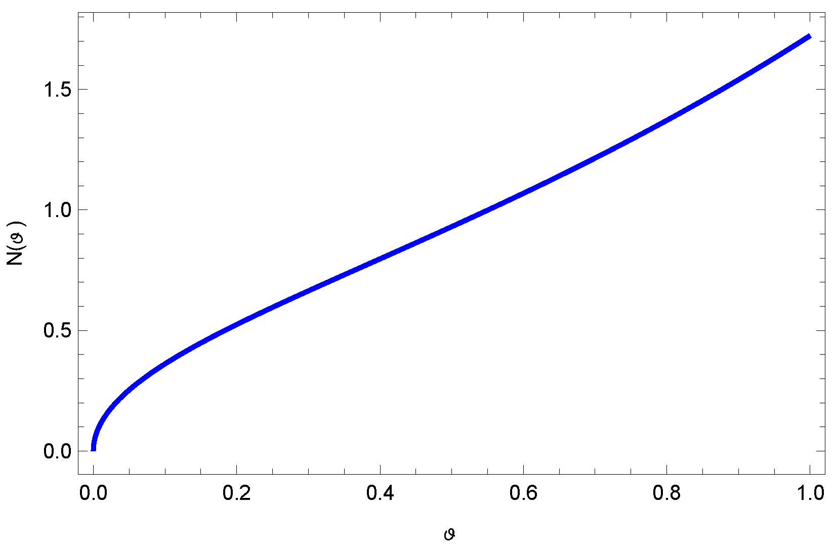
Example 2.

Consider the famous growth model given by

$$a\left({}_{\mathbf{k}}\mathcal{D}_{0^{+}}^{(\varrho ,\lambda )}N\right)\left(\zeta \right)-N\left(\zeta \right)=0,$$

(23)

which is subject to the condition

$$\left({}_{\mathbf{k}}\mathcal{I}_{0^{+}}^{(nk-\varrho ,\lambda )}N\right)\left(0\right)=d_0,$$

where $\lambda ,\varrho \ge 0$, $a,b\in R(a\ne 0)$, $\mathbf{k}>0$, $n=\left[{\displaystyle \frac{\varrho }{\mathbf{k}}}\right]=1$. The solution to (23) is given by

$$N\left(\vartheta \right)=d_0\sum _{m=0}^{\infty }{\displaystyle \frac{e^{-\lambda (\vartheta -a)}}{{\Gamma }_{\mathbf{k}}(\varrho +m\varrho )}}{(\vartheta -a)}^{{\displaystyle \frac{(m+1)\varrho }{\mathbf{k}}}-1}.$$

(24)

By selecting $b=c=1,N_0=0$ and $\beta =0$ in (20) and $a=0,d=d_0$ in (21), we obtain the growth model with a solution that is given in (24). Furthermore, with the parameters $\mathbf{k}=1,\lambda =0,\varrho =1.5$ and $d_0=1$, we obtain

$$N\left(\vartheta \right)=\sum _{m=0}^{\infty }{\displaystyle \frac{{\left(\vartheta \right)}^{1.5m+0.5}}{\Gamma \left(\right(1+m\left)1.5\right)}}.$$

(25)

The graph of the function $N\left(\vartheta \right)$ is shown in the following Figure 2.

8. Conclusions

In current times, fractional calculus has gained significant attention due to its broad application in various scientific fields. This study introduces a new form of a TRLF integral operator, which covers many definitions of fractional integrals. The novel TRLF fractional derivative operator is defined to encompass many well-known forms of fractional derivatives listed in the literature on fractional calculus. Additionally, we investigated the fundamental properties of the newly defined fractional operators of differentiation and integration. Our research article focused on many features, including the boundedness of a new form of TRLF operators to support the validity of our findings. We also provided pictorial representations of their growth model (25). The LT of novel operators was evaluated. Furthermore, the LT was used to evaluate the solution of the fractional kinetic Equation (20) with given conditions. In addition, we discussed the Hyers–Ulam stability in the context of our new form of TRLF operators. Moreover, tempered operators provided a more realistic modeling framework for systems with fading memory effects, in which past influence decays at a controlled, exponential rate. This flexibility improves their applicability for physical processes with localized memory and enhances the accuracy of modeling complex dynamical systems. These results provide researchers with a solid foundation for the further exploration of related subjects. Future research using this paper’s approach could explore topics such as new forms of TRLF differential equations formed by a combination of different TRLF operators.

References

- Novozhenova, O.G. Life And Science of Alexey Gerasimov, One of the Pioneers of Fractional Calculus in Soviet Union. Fract. Calc. Appl. Anal. 2017, 20, 790–809. [Google Scholar] [CrossRef]
- Caputo, M.; Fabrizio, M. On the notion of fractional derivative and applications to the hysteresis phenomena. Meccanica 2017, 52, 3043–3052. [Google Scholar] [CrossRef]
- Abel, N.H. Solution de quelques problemes l’aide d’integrales definies. Mag. Naturv. 1823, 1, 11–27. [Google Scholar]
- Engheta, N. On fractional calculus and fractional multipoles in electromagnetism. IEEE Trans. Antennas Propag. 1996, 44, 554–566. [Google Scholar] [CrossRef]
- Alcoutlabi, M.; Martinez-Vega, J. Application of fractional calculus to viscoelastic behaviour modelling and to the physical ageing phenomenon in glassy amorphous polymers. Polymer 1998, 39, 6269–6277. [Google Scholar] [CrossRef]
- Kulish, V.V.; Lage, J.L. Application of fractional calculus to fluid mechanics. J. Fluids Eng. 2002, 124, 803–806. [Google Scholar] [CrossRef]
- Tarasov, V.E. Handbook of Fractional Calculus with Applications; de Gruyter: Berlin, Germany, 2019. [Google Scholar]
- Mainardi, F. Fractional Calculus and Waves in Linear Viscoelasticity: An Introduction to Mathematical Models; World Scientific: Singapore, 2022. [Google Scholar]
- Magin, R.L. Fractional calculus models of complex dynamics in biological tissues. Comput. Math. Appl. 2010, 59, 1586–1593. [Google Scholar] [CrossRef]
- Bhrawy, A.H.; Taha, T.M.; Machado, J.A.T. A review of operational matrices and spectral techniques for fractional calculus. Nonlinear Dyn. 2015, 81, 1023–1052. [Google Scholar] [CrossRef]
- Kilbas, A.; Srivastava, H.M.; Trujillo, J.J. Theory and Applications of Fractional Differential Equations; Elsevier: Amsterdam, The Netherlands, 2006. [Google Scholar]
- Magin, R.L. Critical Reviews™ in Biomedical Engineering; Begell Digital Portal: Chicago, IL, USA, 2004. [Google Scholar]
- Oldham, K.B.; Spanier, J. The Fractional Calculus; Academic Press: New York, NY, USA, 1974. [Google Scholar]
- Baleanu, D.; Diethelm, K.; Scalas, E.; Trujillo, J.J. Fractional Calculus, Models and Numerical Methods; World Scientific: Singapore, 2012. [Google Scholar]
- Uchaikin, V.V. Fractional Derivatives for Physicists and Engineers. Volume I. Background and Theory; Springer: Berlin/Heidelberg, Germany, 2013; p. 373. [Google Scholar] [CrossRef]
- Samko, S.G.; Kilbas, A.A.; Marichev, O.I. Fractional Integrals and Derivatives, Theory and Applications; Gordon and Breach Science Publishers: New York, NY, USA, 1993. [Google Scholar]
- Buschman, R.G. Decomposition of an integral operator by use of Mikusinski calculus. SIAM J. Math. Anal. 1972, 3, 83–85. [Google Scholar] [CrossRef]
- Meerschaert, M.M.; Sikorskii, A. Stochastic Models for Fractional Calculus; Walter de Gruyter GmbH & Co. KG: Berlin, Germany, 2011; Volume 43. [Google Scholar]
- Srivastava, H.M.; Buschman, R.G. Convolution Integral Equations with Special Function Kernels; Wiley Eastern: New York, NY, USA, 1977. [Google Scholar]
- Diaz, R.; Pariguan, E. On hypergeometric functions and pochhammer k-symbol. Divulg. Math. 2007, 15, 179–192. [Google Scholar]
- Li, C.; Deng, W.; Zhao, L. Well-posedness and numerical algorithm for the tempered fractional ordinary differential equations. Discret. Contin. Dyn. Syst. Ser. B 2019, 24, 1989–2015. [Google Scholar]
- Sabzikar, F.; Meerschaert, M.M.; Chen, J. Tempered fractional calculus. J. Comput. Phys. 2015, 293, 14–28. [Google Scholar] [CrossRef] [PubMed]
- Baeumera, B.; Meerschaert, M.M. Tempered stable Levy motion and transient super-diffusion. J. Comput. Appl. Math. 2010, 233, 2438–2448. [Google Scholar] [CrossRef]
- Cartea, A.; del-Castillo-Negrete, D. Fluid limit of the continuous-time random walk with general Levy jump distribution functions. Phys. Rev. E 2007, 76, 041105. [Google Scholar] [CrossRef]
- Podlubny, I. Fractional Differential Equations; Academic Press: New York, NY, USA, 1999. [Google Scholar]
- Jarad, F.; Abdeljawad, T. Generalized fractional derivatives and Laplace transform. Discret. Contin. Dyn. Syst. Ser. B 2020, 13, 709–722. [Google Scholar] [CrossRef]
- Mubeen, S.; Habibullah, G.M. k-Fractional integrals and application. Int. J. Contemp. Math. Sci. 2012, 7, 89–94. [Google Scholar]
- Romero, L.G.; Luque, L.L.; Dorrego, G.A.; Cerutti, R.A. On the k-Riemann-Liouville fractional derivative. Int. J. Contemp. Math. Sci. 2013, 8, 41–51. [Google Scholar] [CrossRef]
- Katugampola, U.N. A new approach to generalized fractional derivatives. Bull. Math. Anal. Appl. 2011, 6, 1–15. [Google Scholar]
- Chen, M.H.; Deng, W.H. Discretized fractional substantial calculus. Esaim Math. Model. Numer. Anal. 2015, 49, 373–394. [Google Scholar]
- Turgeman, L.; Carmi, S.; Barkai, E. Fractional Feynman-Kac equation for non-Brownian functionals. Phys. Rev. Lett. 2009, 103, 190201. [Google Scholar] [CrossRef]
- Khan, H.; Alzabut, J.; Baleanu, D.; Alobaidi, G.; Rehman, M.U. Existance of solutions and numerical scheme for a generalized hybrid class of n-coupled modified ABC-fractional differential equations with an application. AIMS Math. 2022, 8, 6609–6625. [Google Scholar] [CrossRef]
- Pepe, P. On Liapunov–Krasovskii functionals under caratheodory conditions. Automatica 2007, 43, 701–706. [Google Scholar] [CrossRef]
- Hilfer, R.; Anton, L. Fractional master equations and fractal time random walks. Phys. Rev. E 1995, 51, 848–851. [Google Scholar] [CrossRef] [PubMed]