Multi-Objective Optimization of a Fractional-Order Lorenz System

Abstract

A fractional-order Lorenz system is optimized to maximize its maximum Lyapunov exponent and Kaplan-York dimension using the Non-dominated Sorting Genetic Algorithm II (NSGA-II) algorithm. The fractional-order Lorenz system is integrated with a recent process called the “modified two-stage Runge-Kutta” (M2sFRK) method, which is very fast and efficient. A Pseudo-Random Number Generator (PRNG) was built using one of the optimized systems that was obtained. The M2sFRK method allows for obtaining a very fast optimization time and also designing a very efficient PRNG with linear complexity, $O\left(n\right)$. The designed PRNG generates 24 random bits at each iteration step, and the random sequences pass all the National Institute of Standards and Technology (NIST) and TestU01 statistical tests, making the PRNG suitable for cryptographic applications. The presented methodology could be extended to any other chaotic system.

1. Introduction

The definition of the Lyapunov exponent is the measurement of the average rate of exponential divergence or convergence of very near trajectories in the phase space of a given chaotic system. One may desire a chaotic system design with a high value in its maximum Lyapunov exponent (MLE); a chaotic system with this characteristic will be more unpredictable or will have more complicated trajectories in its phase space.

In this work, a multi-objective optimization of a fractional-order Lorenz system is presented; the values of its MLE and the Kaplan-York dimension (KYD) are maximized. The constants related to the fractional-order Lorenz system are the parameters that are varied to maximize the value of the MLE and KYD.

Chaotic systems are widely used in various fields, such as image encryption [1,2,3,4] , secure communication [4,5], speech encryption [6], pseudo-random number generators [7,8,9,10], or the design of hash functions [11]. Furthermore, in recent years, a lot of work in the area of Automatic Control has been conducted related to parameter estimation using heuristics for fractional-order systems [12]. The optimization of the parameters of fractional-order controllers for load frequency stabilization in power networks has also been carried out [13] using heuristics.

In [2], the authors designed a PRNG with three different fractional chaotic systems, namely a fractional Chen system, a Lu system, and a fractional generalized double-humped logistic map.

In [4] (p. 128), the multi-objective optimization of a commensurate fractional Lorenz system is presented, aiming to maximize both the MLE and the KYD. In [4] (p. 128), Grünwald-Letnikov approximation is used to integrate the fractional Lorenz system with a short memory size equal to 64. The running time of the optimization process was 63 min in a 2.6 GHz Intel Core i5 machine. As will be shown in this work, simulation time can be reduced to seconds when using a novel two-step integration method called M2sFRK [14].

In [3], the three parameters of the Chen system were optimized using the NSGA-II multi-objective optimization algorithm. The obtained MLEs have a value of less than 3.0. Here, again, the Grünwald–Letnikov method was used to integrate the fractional chaotic system.

In [15], a chaotic cellular neural network was optimized by maximizing only its KYD. The Grünwald–Letnikov method was used to integrate the cellular neural network.

In [16], three different fractional systems were also optimized using the maximization of the KYD as the single objective function; the FDE12 MatLab function was used to integrate the systems. One of the conclusions of the study was that simulation time is the bottleneck in the simulation of fractional-order chaotic oscillators.

As computational time is an import issue in the simulation of fractional-order systems, a recently modified Runge-Kutta method [14,17] has been used (the M2sFRK method), which consists of only two evaluations of the system equations; thus, M2sFRK is even simpler than the fourth-order Runge-Kutta method used to integrate systems with integer derivatives. Therefore, using the M2sFRK method reduces the optimization time of the Lorenz system to only a few seconds and also allows for building efficient Pseudo-Random Number Generators with linear complexity, as will be shown later in this work.

The rest of this work is organized as follows: In Section 2, all the methodology used to simulate and optimize the fractional-order Lorenz system is explained. In Section 3, the application of one optimized system to generate pseudo-random sequences of binary numbers is explained. To show that the presented methodology can be applied to other systems, the Arneodo system was also optimized in Section 4. Section 5 provides some discussion about this work. Finally, Section 6 concludes this paper briefly.

2. Optimization Methodology

In this section, the fractional Lorenz system, the M2sFRK method used to integrate it, and the multi-objective optimization of its parameters to maximize its MLE and KYD will be described.

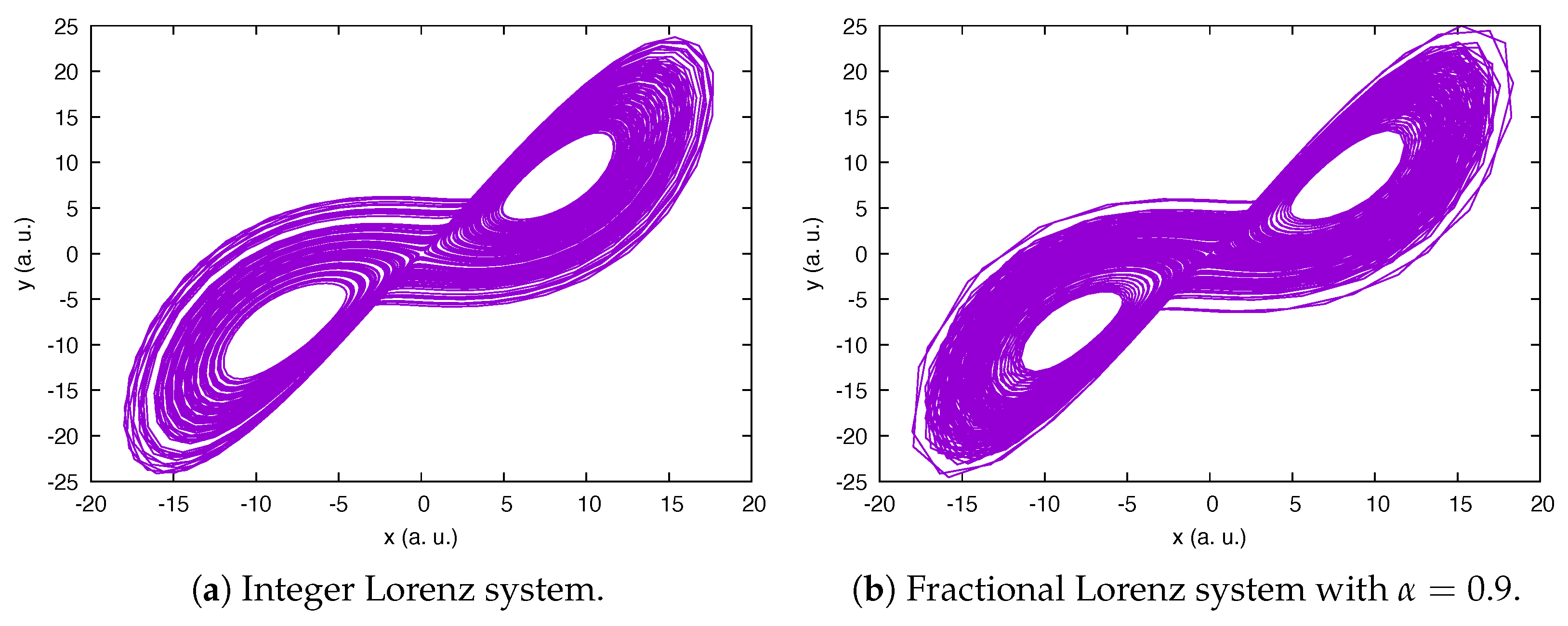
2.1. The Fractional Lorenz System

The fractional Lorenz system is described as

$$\begin{array}{cc}\hfill D^{\alpha }x& =\sigma (y-x),\hfill \\ \hfill D^{\alpha }y& =x(\rho -z)-y,\hfill \\ \hfill D^{\alpha }z& =xy-\beta z,\hfill \end{array}$$

(1)

where x, y, and z are the three state variables, $\alpha$ represents the fractional derivative, and, in this case, $\alpha <1$. Common values for the constant parameters $(\sigma ,\rho ,\beta )$ are $(10,28,8/3)$, which were used in the simulations of the integer-order Lorenz system.

The Lyapunov exponents (LEs) were calculated using the method in [18]. This method is similar to the classical method [19], which involves Gram–Schmidt orthonormalization and the calculation of perturbation-length logarithms. Once the LEs were calculated, the KYD was calculated by evaluating (2), where k is an integer, and the LEs are ordered so that the most positive or largest becomes ${\mathrm{LE}}_1$; j is the largest index, for which the sum of the LEs is equal to or greater than zero. All the implementation was coded in the C programming language.

$$\mathrm{KYD}=k+{\displaystyle \frac{{\sum }_{i=1}^j{\lambda }_i}{|{\lambda }_{j+1}|}}$$

(2)

2.2. The M2sFRK Method for Fractional Integration

The M2sFRK method is described in [14] and is reproduced here for clarity purposes. This is a two-stage explicit fractional Runge-Kutta method defined as

$$y_{k+1}=y_k+K_2,\mathrm{for}k=0,1,\dots M-1,$$

(3)

where

$$\begin{array}{cc}\hfill K_1& ={\displaystyle \frac{h^{\alpha }}{\Gamma (\alpha +1)}}f(t_k,y_k),\hfill \\ \hfill K_2& ={\displaystyle \frac{h^{\alpha }}{\Gamma (\alpha +1)}}f(t_k+c_{2}h,y_k+a_{21}{K}_1),\hfill \\ \hfill a_{21}& ={\displaystyle \frac{\Gamma {(\alpha +1)}^2}{\Gamma (2\alpha +1)}},\hfill \\ \hfill c_2& =a_{21}^{1/\alpha },\hfill \end{array}$$

(4)

$\alpha$ is the fractional derivative value, and h is the integration step. As the fractional Lorenz system in Equation (1) does not depend on time, the calculation of constant $c_2$ is not needed. Thus, to integrate Equation (1), the M2sFRK method is

$${\mathbf{v}}_{k+1}={\mathbf{v}}_k+{\mathbf{K}}_2,\mathrm{for}k=0,1,\dots M-1,$$

(5)

where

$$\begin{array}{cc}\hfill {\mathbf{K}}_1& ={\displaystyle \frac{h^{\alpha }}{\Gamma (\alpha +1)}}\mathbf{f}({\mathbf{v}}_k),\hfill \\ \hfill {\mathbf{K}}_2& ={\displaystyle \frac{h^{\alpha }}{\Gamma (\alpha +1)}}\mathbf{f}({\mathbf{v}}_k+a_{21}{\mathbf{K}}_1),\hfill \\ \hfill a_{21}& ={\displaystyle \frac{\Gamma {(\alpha +1)}^2}{\Gamma (2\alpha +1)}},\hfill \end{array}$$

(6)

where $\mathbf{v}={[x,y,z]}^{\mathrm{T}}$, ${\mathbf{K}}_1$, and ${\mathbf{K}}_2$ are also three-dimensional vectors. $\mathbf{f}$ is the function of the fractional system in (1).

2.3. The Optimization of the Fractional Lorenz System

The x-y phase space of the integer Lorenz system is shown in Figure 1a, and in Figure 1b, the same phase space is shown for the fractional-order Lorenz system for $\alpha =0.9$. The parameter values used for both systems are $(\sigma ,\rho ,\beta )$ = $(10,28,8/3)$. The integration step was set equal to $0.01$. To obtain Figure 1a, the fourth-order Runge-Kutta method was used. To obtain Figure 1b, the method described in Equation (6) was used. Here, it is important to note that the method in Equation (6) is an approximation that maintains the chaotic behavior in the fractional Lorenz system. The Lyapunov spectrum for the fractional Lorenz system is shown in Figure 2 for $\alpha \in [0.80,0.99]$.

Now that the above makes it possible to simulate and calculate the Lyapunov exponents of the fractional Lorenz system, the goal is to search its parameter values $[\sigma ,\rho ,\beta ]$ that maximize the MLE and KYD. This is a multi-objective optimization problem, where there is no unique solution; the solution is a set of them. The search space was set equal to $\sigma \in [1,300]$, $\rho \in [1,120]$, and $\beta \in [1,300]$. The search was limited to within four decimal places for all three variables.

To calculate the Lyapunov spectrum, the initial condition $[x_0=5,y_0=10,z_0=15]$ was set, with a transient time of 5 s, and 2000 iterations were used; measurements were taken at every two integration steps. The LEs for the original Lorenz system with $\alpha =0.9$ are $[0.964239,-0.016463,-14.614443]$, with KYD = 2.064852. Figure 3 shows the solutions found by the NSGA-II algorithm for three different seeds. A population of 40 solutions and 500 generations were set for the search for the NSGA-II algorithm.

The phase portraits for x-y and y-z for the solution $[\sigma =19.5133$, $\rho =119.5466$, $\beta =4.17380]$ with MLE = 3.272982 and KYD = 2.087540 are shown in Figure 4. The 10 different solutions, with MLE $>2.5$, corresponding to the ones shown in Figure 3, are listed in

Table 1. Ten solutions taken from Figure 3 with MLE $>3$.

MLE	KYD	$\mathit{\sigma }$	$\mathit{\rho }$	$\mathit{\beta }$
3.714313	2.009484	32.5167	118.9399	7.7136
3.661470	2.048009	29.8022	118.9523	6.0606
3.534711	2.054591	26.8531	119.4898	5.8574
3.512003	2.081190	23.1857	117.3934	4.4772
3.440673	2.083289	23.1105	116.9628	4.1644
3.420663	2.082792	23.1857	117.3934	4.1344
3.286999	2.083993	23.1857	117.0897	4.1344
3.174116	2.088680	21.9799	119.9868	3.2355
3.159071	2.090405	17.9290	119.3225	4.1486
3.147922	2.110244	17.9290	117.9841	2.8672

.

All the used C program code and found solutions are publicly available at https://delta.cs.cinvestav.mx/~fraga/FracLorenz.tar.gz (accessed on 28 January 2025).

3. Pseudo-Random Number Generator

As an application of the optimized fractional Lorenz system, a Pseudo-Random Number Generator (PRNG) was designed. The solution $[\sigma =19.5133$, $\rho =119.5466$, $\beta =4.1738]$ with MLE = 3.272982 and KYD = 2.087540 was selected; the phase portraits of the oscillator with these parameter values are shown in Figure 4.

To produce a sequence of pseudo-random binary numbers, the value of the output variables $[x,y,z]$ in (1), as these are real numbers, are decomposed with the frexp C programming language function that breaks a floating-point number into its normalized fraction and its power of 2. A real number in the computer is represented as $f\times 2^e$, where f is the normalized fraction with only one binary digit in its integer part, and e is the exponent. Using part f, eight binary digits are generated as

$$b=\left(\lfloor f\times 2^{40}\rfloor \right)\mathrm{mod}256.$$

(7)

This means that each of the three variables (x, y, and z) is multiplied by the big integer $2^{40}$. The result is converted into an integer number, and then the last eight bits (1 byte) in the resulting integer number are taken. The sequence of pseudo-random numbers is generated by concatenating the three generated output bytes at each iteration.

In this way, 100 sequences of ${10}^6$ were generated and passed through the TestU01 [20] and NIST [21] statistical tests. The results are shown in

Table 2. Results of applying 3 TestU01 and 10 NIST statistical tests to 100 sequences of ${10}^6$ bits of the designed PRNG with the fractional Lorenz system.

		PRNG with Real		PRNG with Fixed
		Numbers		Point Arithmetic
	TestU01 test name	–
1	Rabbit	All 40 tests passed		All 40 tests passed
2	Alphabit	All 17 tests passed		All 17 tests passed
3	Block Alphabit	All 6 repetitions of		All 6 repetitions of
		Alphabit tests passed		Alphabit tests passed
	NIST test name	p-value	Proportion	p-value	Proportion
4	Frequency	0.455937	98	0.759756	99
5	BlockFrequency	0.514124	98	0.759756	97
6	CumulativeSums	0.674343	98	0.656132	99
7	Runs	0.304126	100	0.574903	100
8	LongestRun	0.699313	100	0.115387	98
9	Rank	0.002559	98	0.319084	99
10	FFT	0.971699	99	0.191687	98
11	NonOverlappingTemplate	0.487699	99	0.494655	99
12	OverlappingTemplate	0.911413	98	0.978072	97
13	Universal	0.262249	99	0.678686	98
14	ApproximateEntropy	0.637119	100	0.739918	99
15	RandomExcursions	0.349123	100	0.391268	99
16	RandomExcursionsVariant	0.261833	99	0.350938	99
17	LinearComplexity	0.334538	100	0.595549	97
18	Serial	0.539942	99	0.523809	100

. The generated pseudo-random sequences pass all the statistical tests.

The designed PRNG can be applied to encrypt/decrypt any digital data. The encryption process involves generating a sequence of the same length as the input sequence data and then applying the xor operation between both sequences. The decryption process is exactly the same as the encryption process. Xoring data provide the same statistics as the pseudo-random sequence, and the input data also become pseudo-random. One example using the color image mandrill is shown in Figure 5. The pseudo-random sequence was generated using the initial conditions $[x_0,y_0,z_0=6,10,14]$. The input image has a size of $512\times 512$ pixels; then, it was necessary to generate a pseudo-random sequence of $512\times 512\times 3=3·2^{18}$ bytes.

Moreover, it is shown here that it is possible to encrypt text. The following 404 bytes of text were taken from Wikipedia (https://en.wikipedia.org/wiki/Digital_image_processing (accessed on 28 January 2025)):

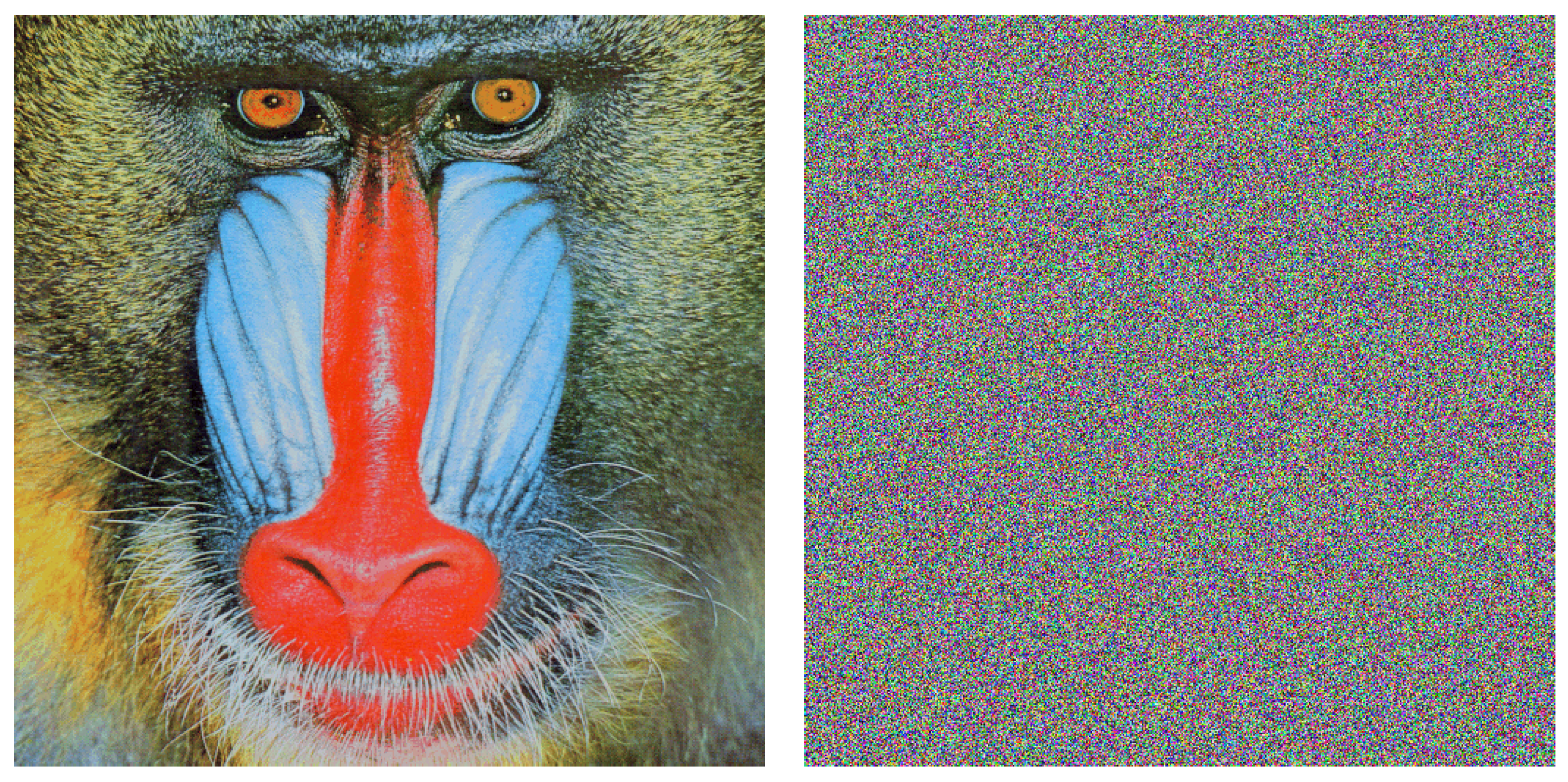
Digital image processing is the use of a digital computer to process digital images through an algorithm [1][2]. As a subcategory or field of digital signal processing, digital image processing has many advantages over analog image processing. It allows a much wider range of algorithms to be applied to the input data and can avoid problems such as the build-up of noise and distortion during processing

This text was encrypted (generated using the same conditions as the mandrill image) and encoded as base64 text to avoid the non-printable characters produced by the encryption process:

xCwi+D3PlGswhKwVJtxU5jx12999kyP9boQUPtXJpqc9LTnomJ/Vg4D3KztmFZTC

R3ax9kiWm4Y5aBMHGQq2V4TsBPoi+07Gmh0SArauoZKb3cSOTDu72YStOq/d0ZGm

odcjqYDSyXs3m9df5AL20ZG3ZaA1SvHq4kn1yoRZO+zoi2/XYsRhYKZqEpuGbssm

B3LYC2EXJeGDeKhhdShm/iR8fXuczfzTfqwA9hNE577SFZQRYYU7k9s9ATge5bNM

HFromDvPxi/g3EhlWoJCl5Fu0/KvfV44AjEpw1pbwfQCZxh8qzMRebL5Nhbcogdt

DwFba30EBCbOg6V4MZbfpk3enkagyhrk2qAcSQ1m6eH9YQ826TyBMY7hO15s4XJh

2+Yl2xOsaeTphcEZqfyDdB7u684o1y2iMBwx6Bs5YGmtYhiLvsGrj/HmPTQe1hcf

D2QX/d4ceK0+OfF//3SwMdLSCINfE6qEInACf2IQtdivihLn9zC2En1NaKB/iPKk

biBkdXJpbmcgcHJvY2Vzc2luZy4=

The PRNG was also implemented in software with fixed-point arithmetic [22] using the number 13.50 (1 bit for the sign, 13 bits for the integer part, and 50 bits for the other fractional part). The binary sequences in this implementation were obtained by concatenating the last eight bits of each variable (x, y, and z). The results of the TestU01 and NIST tests with 100 sequences of ${10}^6$ bits are also shown in Table 2. The minimum representable number is $2^{-50}$. Figure 6 shows the correlation among three pairs of sequences; sequence (1) was generated using initial conditions of $(x_0,y_0,z_0)=(10,10,10)$, sequence (2) was generated using initial conditions of $(x_0,y_0,z_0)=(10+ϵ,10,10)$, and sequence (3) was generated using initial conditions of $(x_0,y_0,z_0)=(10,10+ϵ,10)$; then, the correlation between sequences (1)–(2), (2)–(3), and (1)–(3) were calculated. The generated binary sequences start to be uncorrelated after 25 bytes; thus, these 25 bytes must be discharged to ensure uncorrelated sequences.

4. Optimization of Fractional Arneodo System

To show that it is possible to apply the described methodology to other chaotic systems, the explained methodology was applied to the Arneodo system [14]. This system is described by the equations

$$\begin{array}{cc}\hfill D^{\alpha }x& =y,\hfill \\ \hfill D^{\alpha }y& =z,\hfill \\ \hfill D^{\alpha }z& =-{\gamma }_{1}x-{\gamma }_{2}y-{\gamma }_{3}z+{\gamma }_4{x}^3.\hfill \end{array}$$

(8)

The values used for the constants are ${\gamma }_1=-5.5$, ${\gamma }_2=3.5$, ${\gamma }_3=1$, and ${\gamma }_4=-1$.

For optimization, ${\gamma }_4$ was kept equal to −1, and the other three variables were searched for within the intervals ${\gamma }_1\in [-100,-1]$ and ${\gamma }_2,{\gamma }_3\in [1,200]$. The other parameters were set as $\alpha =0.85$, $h=0.005$, population size: 40 solutions, and 500 generations. The results obtained using three different seeds are shown in Figure 7. Ten solutions taken from Figure 7 are listed in

Table 3. Ten solutions of the optimized Arneodo system taken from Figure 7.

MLE	KYD	${\mathit{\gamma }}_1$	${\mathit{\gamma }}_2$	${\mathit{\gamma }}_3$
1.133314	2.400701	−94.9042	28.0987	1.6709
1.089930	2.422546	−96.0482	29.8352	1.4881
1.060094	2.403057	−94.5423	28.0987	1.6641
1.051732	2.429479	−95.6548	29.8352	1.4881
0.927153	2.461696	−94.4014	34.6392	1.0057
0.894752	2.469233	−94.7296	34.6336	1.0010
0.877517	2.470804	−98.4468	35.9923	1.0031
0.849975	2.482956	−95.1019	34.8128	1.0017
0.803558	2.473915	−94.3803	34.6342	1.0032
0.788414	2.475124	−94.3867	34.6337	1.0031

. This table also shows the obtained parameter values. Four decimal digits are used in Table 3, as is the case in the results for the optimized fractional Lorenz system.

The phase portraits for the oscillator using ${\gamma }_1=-5.5$, ${\gamma }_2=3.5$, and ${\gamma }_3=1$ and the optimized oscillator using parameter values ${\gamma }_1=-98.7515$, ${\gamma }_2=30.3757$, and ${\gamma }_3=1.5161$ (with MLE = 1.134307 and KYD = 2.424701) are shown in Figure 8. A total of 8000 points for each oscillator were used in the graphs in Figure 8. The original Arneodo fractional system used MLE = 1.000358 and KYD = 2.002893, and in Figure 7, one can observe that all the optimized solutions have KYD > 2.4, and some others have MLE > 1.0. The phase portraits of the optimized system shown in Figure 7b have wider ranges than the original in Figure 7a; for variable x, for example, $x\in [-4:4]$ in Figure 7a; this interval is $x\in [-15:15]$ in Figure 7b. The optimized fractional system presents bigger steps and wider coverage of the space than the non-optimized system.

5. Discussion

A comparison of all the possible ways a PRNG can be built is presented in [7]. A single reference [23] is presented of a PRNG based on fractional chaos. In the comparison results, the authors of [7] mention that the complexity of the fractional design is $O\left(n^2\right)$, and the second poorer bit rate is 4.512 Mbit/s. The reduced performance is because the system state at iteration n is obtained by solving the system for the previous $n-1$ states. The proposed PRNG design has the complexity $O\left(n\right)$, which is comparable to the other possible designs of a PRNG shown in [7]. It is expected that the hardware design of the presented fractional PRNG will be very efficient with a very high bit rate of pseudo-random bits.

As the modified Runge-Kutta method used in this work consists of only two steps, it is even more efficient than the fourth-order Runge-Kutta method for solving integer-order systems. The optimization time was 7 s when using a MacBook with an M2 processor, with 40 solutions and 500 generations; this means that the optimization process evaluates $40\times 500=20,000$ times the function that measures the Lyapunov exponents. The optimization in [4] (p. 128) took 63 min to evaluate a similar objective function 4000 times.

The seed for the designed PRNG is the initial values $(x_0,y_0,z_0)$. It is not completely clear how many different values can be used for the seed. It is necessary to analyze the domain of attraction of the fractional system in three dimensions and find the ranges for each variable where the system oscillates. Even so, it is not clear how many values a floating-point variable can have within a given range. If the PRNG is implemented using fixed-point arithmetic, then the exact number of different seed values can be calculated [8].

The fixed-point arithmetic implementation uses the number 13.50, with 1 sign bit, 13 bits for the integer part, and 50 bits for the fractional part. The domain of attraction was calculated for $x_0\in [-128,128]$, $y_0\in [-128,128]$, and $z_0=9$ and is shown in Figure 9a. In Figure 9b,c, the domain of attractions for the same ranges in $x_0$ and $y_0$ are shown but for $z_0=10$ and $z_0=11$, respectively. If it is supposed that there are no discontinuities among the shown domain of attractions, then the ranges in which the variables can start are $x_0,y_0\in [-32,32]$ and $z_0\in [9,11]$. Then, the key size is equal to $(2^6·2^{50})·(2^6·2^{50})$$·(2^2·2^{50})$$=2^{112+52}=2^{164}$. This key size is equal to the number of different seeds that the PRNG can have.

6. Conclusions

The M2sFRK method was used to integrate a fractional Lorenz system. This method has only two single steps and is, therefore, very efficient and computationally fast. Then, the three parameters $\sigma$, $\rho$, and $\beta$ of the fractional Lorenz system were optimized to maximize their maximum Lyapunov exponent and its Kaplan-York dimension. The multi-objective NSGA-II algorithm was used to perform the optimization.

For one of the optimized fractional systems, a PRNG was designed, and two PRNGs were implemented: one using real numbers and the other using fixed-point arithmetic. The produced pseudo-random sequences pass all the TestU01 and NIST statistical tests, which makes the designed PRNG suitable for cryptographic applications. The encryption of a color image and a single piece of text are shown as two possible applications of the designed PRNG.

Future work could involve a hardware design for the presented PRNG, as it could be used in an FPGA.

References

1. Yang, C.H.; Lee, J.D.; Tam, L.M.; Cheng, S.C. FPGA Implementation of Image Encryption by Adopting New Shimizu–Morioka System-Based Chaos Synchronization. Electronics 2025, 14, 740. [Google Scholar] [CrossRef]
2. Yang, C.; Taralova, I.; El Assad, S.; Loiseau, J. Image encryption based on fractional chaotic pseudo-random number generator and DNA encryption method. Nonlinear Dyn. 2022, 109, 2103–2127. [Google Scholar] [CrossRef]
3. Guillén-Fernández, O.; Tlelo-Cuautle, E.; de la Fraga, L.; Sandoval-Ibarra, Y.; Nuñez-Perez, J.C. An Image Encryption Scheme Synchronizing Optimized Chaotic Systems Implemented on Raspberry Pis. Mathematics 2022, 10, 1907. [Google Scholar] [CrossRef]
4. Tlelo-Cuautle, E.; de la Fraga, L.; Guillén-Fernández, O.; Silva-Juárez, A. Optimization of Integer/Fractional Order Chaotic Systems by Metaheuristics and their Electronic Realization; CRC Press: Boca Raton, FL, USA, 2021. [Google Scholar]
5. Yan, S.; Lu, R.; Zhang, H. Dynamical behaviors of the simple chaotic system with coexisting attractors and its synchronous application. Integration 2025, 102, 102368. [Google Scholar] [CrossRef]
6. Bonny, M.A.T.; Sambas, A.; Vaidyanathan, S.; Al Nassan, W.; Zhang, S.; Obaideen, K.; Mamat, M.; Kamal, M. A Speech Cryptosystem Using the New Chaotic System with a Capsule-Shaped Equilibrium Curve. Comput. Mater. Contin. 2023, 75, 5987–6006. [Google Scholar] [CrossRef]
7. AbdELHaleem, S.H.; Abd-El-Hafiz, S.K.; Radwan, A.G. Analysis and Guidelines for Different Designs of Pseudo Random Number Generators. IEEE Access 2024, 12, 115697–115715. [Google Scholar] [CrossRef]
8. de la Fraga, L.G.; Ovilla-Martínez, B. Generating pseudo-random numbers with a Brownian system. Integration 2024, 96, 102135. [Google Scholar] [CrossRef]
9. Yu, F.; Zhang, S.; Su, D.; Wu, Y.; Musoya Gracia, Y.; Yin, H. Dynamic Analysis and Implementation of FPGA for a New 4D Fractional-Order Memristive Hopfield Neural Network. Fractal Fract. 2025, 9, 115. [Google Scholar] [CrossRef]
10. Naik, R.; Singh, U. A Review on Applications of Chaotic Maps in Pseudo-Random Number Generators and Encryption. Ann. Data Sci. 2024, 11, 25–50. [Google Scholar] [CrossRef]
11. Xing, H.; Min, R.; Li, S.; Yang, Z.; Yang, Y. Hyperchaotic hashing: A chaotic hash function based on 2D linear cross-coupled map with parallel feedback structure. Sci. Rep. 2025, 15, 5462. [Google Scholar] [CrossRef] [PubMed]
12. Nassef, A.; Abdelkareem, M.; Maghrabie, H.; Baroutaji, A. Metaheuristic-Based Algorithms for Optimizing Fractional-Order Controllers—A Recent, Systematic, and Comprehensive Review. Fractal Fract. 2023, 7, 553. [Google Scholar] [CrossRef]
13. Latif, A.; Suhail Hussain, S.; Chandra Das, D.; Selim Ustun, T.; Iqbal, A. A review on fractional order (FO) controllers’ optimization for load frequency stabilization in power networks. Energy Rep. 2021, 7, 4009–4021. [Google Scholar] [CrossRef]
14. Sai Lekshmi, A.; Balakumar, V. Numerical investigation of fractional order chaotic systems using a new modified Runge-Kutta method. Phys. Scr. 2024, 99, 105225. [Google Scholar] [CrossRef]
15. Tlelo-Cuautle, E.; González-Zapata, A.; Díaz-Muñoz, J.; de la Fraga, L.; Cruz-Vega, I. Optimization of fractional-order chaotic cellular neural networks by metaheuristics. Eur. Phys. J. Spec. Top. 2022, 231, 2037–2043. [Google Scholar] [CrossRef] [PubMed]
16. Silva-Juárez, A.; Tlelo-Cuautle, E.; de la Fraga, L.; Li, R. Optimization of the Kaplan-Yorke dimension in fractional-order chaotic oscillators by metaheuristics. Appl. Math. Comput. 2021, 394, 125831. [Google Scholar] [CrossRef]
17. Ghaffari, R.; Saad, N. Fractional Order Runge–Kutta Methods. Fractal Fract. 2023, 7, 245. [Google Scholar] [CrossRef]
18. Balcerzak, M.; Pikunov, D.; Dabrowsk, A. The fastest, simplified method of Lyapunov exponents spectrum estimation for continuous-time dynamical systems. Nonlinear Dyn. 2018, 94, 3053–3065. [Google Scholar] [CrossRef]
19. Parker, T.; Chua, L. Practical Numerical Algorithms for Chaotic Systems; Springer: Berlin/Heidelberg, Germany, 1989. [Google Scholar]
20. Ecuyer, L.; Simard, R.; TestU01: A C Library for Empirical Testing of Random Number Generators. ACM Transactions on Mathematical Software. 2007, Volume 33. Available online: http://simul.iro.umontreal.ca/testu01/tu01.html (accessed on 28 January 2025).
21. Rukhin, A.; Soto, J.; Nechvatal, J.; Smid, M.; Barker, E.; Leigh, S.; Levenson, M.; Vangel, M.; Banks, D.; Heckert, A.; et al. A Statistical Test Suite for the Validation of Random Number Generators and Pseudo Random Number Generators for Cryptographic Applications. 27 April 2010. Available online: http://csrc.nist.gov/groups/ST/toolkit/rng/documentation_software.html (accessed on 28 January 2025).
22. Yates, R. Fixed-point arithmetic: An introduction. Digit. Sig. Labs 2009. Available online: https://www.cpplab.net/web/dsp/fp.pdf (accessed on 28 January 2025).
23. AbdElHaleem, S.H.; Abd-El-Hafiz, S.K.; Radwan, A.G. Secure blind watermarking using fractional-order Lorenz system in the frequency domain. AEU-Int. J. Electron. Commun. 2024, 173, 154998. [Google Scholar] [CrossRef]
Figure 1. Phase space for the x-y variables of the integer and fractional Lorenz systems.
Fractalfract 09 00171 g001
Figure 2. Lyapunov exponents for the fractional Lorenz system for α [ 0.8 , 1 ] with increments of 0.01.
Fractalfract 09 00171 g002
Figure 3. Solutions in the objective space obtained by the NSGA-II algorithm with three different seeds for its internal pseudo-random number generator.
Fractalfract 09 00171 g003
Figure 4. Phase portraits of the selected optimized fractional Lorenz system.
Fractalfract 09 00171 g004
Figure 5. The test image “mandrill” and its encryption with the designed fractional PRNG.
Fractalfract 09 00171 g005
Figure 6. Correlation between three sequences. Check the details in the text.
Fractalfract 09 00171 g006
Figure 7. Solutions obtained by NSGA-II using three different seeds to maximize the MLE and KYD of the Arneodo system with α = 0.85 and h = 0.005 .
Fractalfract 09 00171 g007
Figure 8. Phase portraits of the original Arneodo oscillator without optimization in (a) and of one optimized oscillator in (b) with the parameters γ 1 = 98.7515 , γ 2 = 30.3757 , and γ 3 = 1.5161 .
Fractalfract 09 00171 g008
Figure 9. Domains of attraction for the fractional Lorenz system implemented using fixed-point arithmetic. A total of 8000 points with the initial conditions of ( x 0 , y 0 ) = ( 10 , 10 ) and the z 0 are shown in each figure and are used for the super-imposed phase portrait in the domain of attraction.
Fractalfract 09 00171 g009