Applying a Gain Scheduled Fractional Order Proportional Integral and Derivative Controller to a Quadratic Buck Converter

Abstract

This work presents a fractional order Proportional Integral and Derivative controller with adaptation characteristics in the control parameters depending on the required output, gain scheduling fractional order PID (GS-FO-PID). The fractional order PID is applied to the voltage control of a DC–DC buck quadratic converter (QBC). The DC–DC buck quadratic converter is designed to operate at 12 V, although in the simulation tests, the output voltage ranges from 5 to 36 V. The performance of the GS-FO-PID is compared with the one from a classic PID. The GS-FO-PID presents better performance when the reference voltage is changed. In the same way, the behavior of the converter with the reference fixed to 12 V output is analyzed with load changes; for this case, the amplitude value of the ripple when the converter is driven by the GS-FO-PID almost has no variation.

1. Introduction

Recent advances in the design and construction of DC converters have made great strides in improving power conversion technologies. Included in these advancements are DC ports with a good high voltage, gain ratio, bidirectional conversion capability, and higher overall efficiency. These advances have been very important, especially for applications in renewable sources, storage systems, microgrids, and power electronics [1,2,3,4]. In the area of power conversion, there is a wide range of DC–DC converter configurations, given the growing demand for improved efficiency as well as versatility for use in various applications. In this regard, notable advances have been made in the design of transformerless DC–DC converters, which offer tangible benefits in terms of weight, size, and even cost reductions. A notable innovation in this domain is the transformerless quadratic step-down converter, known for its high-voltage gain ratio and continuous input/output current ports [3]. The DC–DC converters are usually placed between a primary power supply and a load. The input includes direct voltage loads capable of powering various digital electronic devices. The system shows nonlinear characteristics due to its variable structure. To address this problem, nonlinear control methods have been used under conditions of time-varying perturbations and load changes [5,6,7].

Different types of DC–DC converters have been designed, including buck, boost, and buck–boost converters. These converters employ a frequency element for voltage conversion, in conjunction with a diode, plus an inductor and a capacitor. In particular, the buck converter changes a DC input voltage into a lower DC output voltage. This converter is a primary circuit in voltage reducing applications. Theoretically, the voltage conversion ratio (gain) of the buck converter (Vo/Vin) operating in continuous conduction mode (CCM) depends only on the duty cycle (d) of the power switch. The d will vary from 0 to 1, so a wide range of reducing gain is possible [8]. However, it has been found that in practice, the gain of the buck converter is normally limited to at least one-tenth. This is because a very small duty cycle would reduce the driving time of the power switch, and at a very high switching frequency, such a short driving time might not be enough for the switch to function properly. To achieve the large voltage reduction with the extended duty cycle, two or more step-down converters can be connected in series. However, if the cascade approach is followed, the array would require multiple switches. On the other hand, cascaded step-down converter arrays have low efficiency. Proposals for N-stage cascade reducer converters with a single power switch have been presented in different works [9,10,11]. In these arrays, the voltage reduction ratio is equal to dN. By using a single switch, these converter proposals provide a practical and economical solution for applications seeking to reduce voltage. A quadratic buck converter (QBC) is a subset of the N-stage but single-switch cascade buck converters, with N = 2, which can be considered a double step-down stage.

Although several control techniques have been widely employed in DC–DC converters and their impact on dynamic behavior and change from second order to first order dynamics has been extensively studied, the implications of these techniques are less understood in the realm of cascade converters, which introduce zeros in the transfer function [12].

In recent years, various control techniques have been applied to DC–DC buck converters. For instance, Bonela et al. [13] have introduced a robust non-fragile control approach for these converters that addresses the influence of these uncertainties. This method involves developing a control law that achieves quadratic stabilization of the closed-loop system while also satisfying the H∞ norm constraint for disturbance attenuation. On the topic of robust control, Saavedra et al. [14] have presented a paper with two control design strategies for voltage regulation in a single inductor dual-output DC–DC buck converter system, in which a linear quadratic regulator and a decoupled PI control law were designed to control the power converter system under parametric uncertainties. The controllers are based on a nominal multiple input–multiple output plant model and performance requirements. For their part, Kumari et al. [15] have compared the closed-loop response of a DC–DC buck converter using different optimization strategies such as model predictive control (MPC) and the linear quadratic regulator (LQR). A similar work was published by Raza et al. [16], in which the LQR cost function is converted to the quadratic programming cost function of the MPC. On the other hand, Fetene et al. [17] have proposed a cost-effective observer-based pole placement controller for a PWM voltage-controlled buck converter with a clear step-by-step design approach. The state space averaged model of the DC–DC power converter is used to design pole placement with an integrator compensator and a full state observer. For their part, Nanyan et al. [18] presented an optimal PID controller for the DC–DC buck converter where the sine–cosine algorithm was employed to improve the performance of the converter. Also, novel techniques such as machine learning have been explored [19].

Specifically on the design and control of buck quadratic DC–DC converters, there are recent publications. For example, Trakuldit et al. [8] have published a work where a quadratic buck converter is designed and evaluated. For their part, Lopez-Santos et al. [20] have presented a quadratic buck converter that is applied for battery charging. In that work, a multi-loop controller using three nested loops was used, involving one sliding mode current controller and two conventional PI controllers. On the other hand, Pop et al. [21] have published a paper where the process of designing a controller for a fourth-order buck converter is presented. In this work, after deriving the control-to-output transfer function based on a matrix state space model, an approximation to a second-degree transfer function is made.

A control option that has not been sufficiently studied is to employ a different classical control for each operational condition. The gain scheduling method in conjunction with the PID offers the advantage of rapid control with the characteristic of adaptability to different operating conditions. Furthermore, if fractional calculation characteristics are employed for the integral and proportional modes of the PID controller, the resulting regulator would increase its performance, given its proven improvement in the control of higher-order systems and systems with nonlinearities, among others. Given the above, this study describes the application of a gain scheduling fractional order PID controller to the regulation of a quadratic buck converter. Then the major contributions of this paper are as follows.

•

To present a fractional order Proportional Integral and Derivative controller with adaptation characteristics;

•

To apply a fractional order PID to control the voltage of a DC–DC buck quadratic converter (QBC);

•

To simulate the system with different output voltages and different loads.

This document is structured as follows: Section 2 provides a comprehensive mathematical model for the dynamic quadratic buck converter (QBC) system. These models serve as the foundation for understanding and controlling the QBC system. Both switched and average models are discussed. Then in Section 3, three types of control are discussed, namely classic PID control, gain scheduling PID, and gain scheduling fractional. This is followed by a discussion in Section 4 about the tuning of the controllers and a comparison of the performance of the controllers, with changes in the reference voltage and load. Finally, in Section 5, some conclusions are drafted.

2. Quadratic Buck Switched Converter Model

It is common that the control strategy starts by obtaining a mathematical model. In this case, an averaged model that requires linearization was obtained. Figure 1 shows the ON and OFF states (Figure 1a and Figure 1b, respectively) that are achieved on the basis of the quadratic buck circuits [22].

2.1. ON–OFF Equations

The behavior in the ON state, as depicted in Figure 1a, yields the following equations expressed in terms of the state variables:

$${\displaystyle \frac{{di}_{L_1}}{dt}}={\displaystyle \frac{V_g-v_{C_1}}{L_1}}$$

(1)

$${\displaystyle \frac{{di}_{L_2}}{dt}}={\displaystyle \frac{v_{C_1}-v_{C_2}}{L_2}}$$

(2)

$${\displaystyle \frac{{dV}_{C_1}}{dt}}={\displaystyle \frac{I_{L_1}-I_{L_2}}{C_1}}$$

(3)

$${\displaystyle \frac{{dV}_{C_2}}{dt}}={\displaystyle \frac{I_{L_2}-I_R}{C_2}}$$

(4)

In the OFF state of the quadratic buck converter, as illustrated in Figure 1b, we derive the following equations in the state variables:

$${\displaystyle \frac{{di}_{L_1}}{dt}}={\displaystyle \frac{-v_{C_1}}{L_1}}$$

(5)

$${\displaystyle \frac{{di}_{L_2}}{dt}}={\displaystyle \frac{-v_{C_2}}{L_2}}$$

(6)

$${\displaystyle \frac{{dv}_{C_1}}{dt}}={\displaystyle \frac{i_{L_1}}{C_1}}$$

(7)

$${\displaystyle \frac{{dv}_{C_2}}{dt}}={\displaystyle \frac{i_{L_2}-i_R}{C_2}}$$

(8)

2.2. Quadratic Buck Switched Model

The equation of the state variable is multiplied by U in the ON state and by (1-U) in the OFF state [8,23].

For $i_{L_1}$, in this instance, the state variable is derived from the following equation:

$${\displaystyle \frac{{di}_{L_1}}{dt}}={\displaystyle \frac{V_g}{L_1}}u-{\displaystyle \frac{v_{C_1}}{L_1}}$$

(9)

For $i_{L2}$, the state variable is derived from the equation:

$${\displaystyle \frac{{di}_{L_2}}{dt}}={\displaystyle \frac{v_{C_1}}{L_2}}u-{\displaystyle \frac{v_{C_2}}{L_2}}$$

(10)

For the variable $v_{C1}$, we derive:

$${\displaystyle \frac{{dV}_{C_1}}{dt}}={\displaystyle \frac{-i_{L_2}}{C_1}}u+{\displaystyle \frac{i_{L_2}}{C_1}}$$

(11)

The state variable $v_{C2}$ is obtained as follows:

$${\displaystyle \frac{{dV}_{C_2}}{dt}}={\displaystyle \frac{i_{L_2}}{C_2}}u-{\displaystyle \frac{v_{C_2}}{C_{2}R}}$$

(12)

2.3. Quadratic Buck Average Model

We substitute the variable u with d, and define the state equations as functions as follows.

For the variable $i_{L_1}$,

$$f_1={\displaystyle \frac{d_{iL1}}{dt}}={\displaystyle \frac{V_g}{L_1}}d-{\displaystyle \frac{v_{C1}}{L_1}}$$

(13)

For the variable $I{iL}_2$,

$$f_2={\displaystyle \frac{d_{iL2}}{dt}}={\displaystyle \frac{v_{C1}}{L_2}}d-{\displaystyle \frac{v_{c2}}{L_2}}$$

(14)

For the variable $v_{C1}$,

$$f_3=\frac{d_{VC1}}{dt}=\frac{-i_{L2}}{C_1}d+\frac{i_{L1}}{C_1}$$

(15)

$$f_4={\displaystyle \frac{d_{VC2}}{dt}}={\displaystyle \frac{i_{L2}}{C_2}}d-{\displaystyle \frac{v_0}{C_2\ast R}}$$

(16)

Setting the equations provided earlier to zero yields for the function $f_1$ the following:

$$v_{g}d=v_{C_1}$$

(17)

For the function $f_2$,

$$f_2=v_{C_1}d=V_0$$

(18)

For the function $f_3$, we have:

$$I_{L_2}d=I_{L_1}$$

(19)

Finally, for the function $f_4$,

$$I_{L_2}={\displaystyle \frac{V_0}{R}}$$

(20)

A transfer function, which characterizes the system’s behavior, can now be obtained (37) [22,23].

$$G\left(s\right)={\displaystyle \frac{\left(\left(\frac{v_{C1}}{C_1{C}_2{L}_2}\right)\left(S^2-\left(\frac{D_{IL1L1}}{V_{C1}}\right)S+\left(\frac{1}{L_1}+\frac{D_{vg}}{R_{C1}{V}_{C1}}\right)\right)\right)}{S^4+\left(\frac{1}{{RC}_2}\right)S^3+\left(\frac{D^2{L}_1+L_2-2}{L_1{L}_2}\right)S^2+\left(\frac{D^2{L}_1+L_2}{{C_{1}C}_2{L}_1{L}_{2}R}\right)S+\left(\frac{1}{{C_{1}C}_2{L}_1{L}_{2}R}\right)}}$$

(21)

3. Description of the Controllers

Three controllers were compared in this work, namely a classical PID, a gain scheduling PID, and a gain scheduling fractional order PID.

3.1. Classical PID

PID control is a classical type of control widely used in industry, which incorporates an evaluation of the proportion (P), the integral (I), and the derivative (D) of the error signal to obtain the control signal. Different variations of PID that include nonlinear characteristics have been reported for many years [24]. As a form of comparison, a classical PID control (22) was chosen, which was adjusted by the relay method, which will be discussed later.

$$U\left(s\right)=K\left(E\left(s\right)+{\displaystyle \frac{1}{T_{i}s}}E\left(s\right)+T_{d}sE\left(s\right)\right)$$

(22)

where

U(s) is the control signal;

E(s) is the error of the system;

K is the proportional gain;

Ti is the integral gain;

Td is the derivative gain.

3.2. Gain Scheduling PID

Gain scheduling is a common method used to control nonlinear systems, since it uses linear design methods [25]. Normally, gain scheduled controllers are calculated by conducting an initial linearization of the system to be controlled at a certain scheduling operational point. Subsequently, for every operational point, linear controllers are calculated; each one is acceptable only near to that specific operational point. Then the controller’s parameters are calculated at every operational point selected. In the case of the PID controller, the parameters K, Ti, and Td are selected for each of the operating points. The desired voltage level is detected, then the selected parameters are used. Figure 2 shows a schematic diagram of the GS-PID controller. As can be seen, the identification algorithm block receives the reference signal and the output of the system; with these signals, it calculates the point of operation at which the system is located. This information is the input to the gain scheduling block that determines the values of the control parameters that will be applied in the PID controller.

3.3. Fractional Order Controllers

Fractional calculus is a research area that is over 300 years old. There are multiple applications in various areas. Control theory is an important area of application. During the last 30 years, efforts have been made to implement fractional calculus techniques in control theory [26]. In fractional calculus, the integration and differentiation of the fundamental operator of non-integer order ${}_{a}D_t^{\alpha }$ are generalized, with a and t as the limits of the operation.

Definition 1.

The continuous fractional integro-differential operator has been defined as:

$${}_{a}D_t^{\alpha }=\left\{\begin{array}{c}\begin{array}{ccc}{\displaystyle \frac{d^{\alpha }}{d{t}^{\alpha }}}& :& \alpha >0,\end{array}\\ \begin{array}{ccc}1& :& \alpha =1\end{array}\\ \begin{array}{ccc}{\int }_a^t{\left(d\tau \right)}^{-\alpha }& :& \alpha <0.\end{array}\end{array}\right.$$

(23)

Definition 2.

Caputo’s definition [27] of a fractional derivative can be written as [28]

$${}_{a}D_t^{\alpha }f\left(t\right)={\displaystyle \frac{1}{\mathsf{\Gamma }\left(n-\alpha \right)}}{\int }_a^t{\displaystyle \frac{f^{\left(n\right)}\left(\tau \right)}{{\left(t-\tau \right)}^{\alpha -n+1}}}d\tau$$

(24)

for (n − 1 < α < n). It holds an important property: the initial conditions for fractional order differential equations with Caputo’s derivative are in the same form as integer-order differential equations.

Definition 3.

If we consider $k={\displaystyle \frac{t-a}{h}}$, where a is a real constant, which expresses a limit value, we can write the Grünwald–Letnikov definition as [27]

$${}_{a}D_t^{\alpha }f\left(t\right)=\underset{h\to 0}{\lim }{\displaystyle \frac{1}{h^{\alpha }}}{\sum }_{j=0}^{\left[{\displaystyle \frac{t-a}{h}}\right]}{\left(-1\right)}^j\left(\begin{array}{c}\alpha \\ j\end{array}\right)f\left(t-jh\right)$$

(25)

where [x] means the integer part of x, and a and t are the bounds of operation for ${}_{a}D_t^{\alpha }f\left(t\right)$. This form of definition is very helpful for obtaining a numerical solution of fractional differential equations.

For zero initial conditions and the lower limit a = 0, the Laplace transform of fractional derivatives (Grünwald–Letnikov and Caputo) reduces to [28]:

$$\mathcal{L}\left\{{}_{0}D_t^{\alpha }f\left(t\right)\right\}=s^{\alpha }F\left(s\right)$$

(26)

The fractional differentiation/integration are linear operations:

$${}_{0}D_t^{\alpha }\left(af\left(t\right)+bg\left(t\right)\right)=a{}_{0}D_t^{\alpha }f\left(t\right)+b{}_{0}D_t^{\alpha }g\left(t\right)$$

(27)

This work considered Caputo’s definition.

3.3.1. Fractional Order PID

In recent years, applications of PID controllers with integral and derivative parts of fractional order have been described. Those studies show an improvement in the performance of the controlled systems [29]. For instance, a generalization of the PID controller was proposed by Podlubny [30,31]; that approach included an integrator of order λ and a differentiator of order δ (PI^λD^δ controller), where a better response of this type of controlled was demonstrated in comparison with other classical PID approaches. Frequency domain approaches for fractional order PID controllers have also been studied [32]. Podlubny [31] proposed the fractional order PI^λD^δ (FO-PID controller). In his proposal, the integrator (λ) and the differentiator (δ) operators are real. Equation (28) shows the discrete-time transfer function of this controller

$$C\left(z\right)={\displaystyle \frac{U\left(z\right)}{E\left(z\right)}}=K_p+{\displaystyle \frac{K_i}{{\left(\omega \left(z^{-1}\right)\right)}^{\lambda }}}+K_d{\left(\omega \left(z^{-1}\right)\right)}^{\delta }$$

(28)

where

λ > 0 is a real integral operator;

δ > 0 is a real differential operator;

K_p is a proportional constant;

K_i is a integration constant;

K_d is a differentiation constant;

${\left(\omega \left(z^{-1}\right)\right)}^{\lambda }$ is an equation to produce an integral FO of $\lambda$;

${\left(\omega \left(z^{-1}\right)\right)}^{\delta }$ is an equation to produce a derivative FO of $\delta$.

In Equation (40), taking λ = 1 and δ = 1, a classical PID controller is obtained. If λ = 0 and K_i = 0, a PD^δ controller is found. In summary, all these types of are particular cases of the fractional order controller, which is more flexible and gives an opportunity to better adjust the dynamical properties of a control system [29].

The performance of a controller has a strong dependence on the parameters selected. For instance, in a PID, its parameters are K_p, K_i, and K_d (38). In the case of a fractional order PID, its parameters also include λ (a real integral operator) and δ (a real differential operator). As in all discrete implementations, the sample time selection is crucial.

3.3.2. Gain Scheduling Fractional Order PID

The case of the gain scheduling fractional order PID is similar to the already explained gain scheduling PID, except in this case, there are two more parameters, λ and δ, that must be obtained. Different algorithms have been published to tune fractional order PID controllers [33,34,35,36]. Some methods to tune fractional order PID controllers have been proposed. For instance, Ayres Junior et al. proposed a method that uses pole placement [37]. For their part, Wu et al. presented a tuning method based on probabilistic robustness [38]. For this study, an agreement between rapid response and small overshoot was desired; the technique is based on the one proposed by Awouda and Mamat [39].

3.4. Stability of the Sytem

The stability of systems controlled by fractional regulators has been studied by different authors [40,41,42,43]. In the case of this work, Matignon’s stability theorem could be used for an analysis of stability [44].

Theorem 3.1 (Matignon’s stability theorem) [40,44]. The fractional transfer function $G\left(s\right)={\displaystyle \frac{Z\left(s\right)}{P\left(s\right)}}$ is stable if and only if the following condition is satisfied in the s-plane

$$\left|arg\left({\sigma }_i\right)\right|=q{\displaystyle \frac{\pi }{2}}$$

where $\sigma =s^q$. When s = 0 is a single root of P(s), the system cannot be stable. For $q=1$, this is the classical theorem of pole location in the complex plane: no pole is in the closed right half-plane of the first Riemann sheet.

4. Analysis of System Response Under the Controllers

4.1. Analysis of the System

The inductance value is determined on the basis of the current ripple pattern within the coil. The equation for inductance when the system is in the ON state is depicted by the gradient of the line originating from 0 to DT_s, while the slope between DT_s and T_s defines the coil’s current value in the OFF state. It is convenient to remember that D is the duty cycle and Ts is the working period (inverse of the working frequency, fs). From this,

$$L_1=\frac{D{T}_s{V}_g(1-v_{C1})}{2\Delta I}$$

(29)

and

$$L_2=\frac{D{T}_s{v}_{C1}(1-D)}{2\Delta I}$$

(30)

Capacitors can be calculated using the following equations:

$$C_1=\frac{-D{T}_s{I}_{L1}(1-I_{L2})}{2\Delta v_{C1}}$$

(31)

and

$$C_2=\frac{D{T}_s(i_{L2}-i_R)}{2\Delta v_{C2}}$$

(32)

Considering the analysis shown in Section 2, the duty cycle is

$$D=\sqrt{{\displaystyle \frac{v_0}{V_g}}}$$

(33)

For the analysis presented in this work, the system was designed with the following parameters:

V_g = 48 V (input voltage);

V_o = 12 V (output voltage);

f_s = 100 × 10³ (working frequency);

R_L = 5 ohms (load);

L₁ = 0.144 mH;

L₂ = 0.096 mH;

C₁ = 0.0434 mFd;

C₂ = 0.0434 mFd.

The following operating points were chosen: 5 V, 12 V, 24 V, and 38 V. The system was designed to operate at 12 V, so the duty cycle was calculated for that output voltage, although by changing the operating point and the reference voltage, the duty cycle varied.

4.2. Tuning PID Controllers

Using the system’s transfer function, the controller was tuned for each operating point.

A relay is used to control the system when it is in a steady state; this causes an oscillation in the system. Using the descriptive function, the critical gain of the system can be calculated [45]. On the other hand, the oscillation frequency of the system under the relay is considered the critical frequency. The plant is then fed with a step while it is regulated with only proportional control. The proportional gain value is calculated using the Ziegler and Nichols tables [24]. From the curve of response of the system, considering a second-order plant, W_n and $\zeta$ are obtained. To apply this method, the system must have overshooting, which is the case. With the data of the system reduced to the second order, using pole placement, the PID values are adjusted. This method was applied directly to the model circuit of Simulink^©.

The tuning algorithm is programmed in a S function. For it to operate, it is necessary for the plant to have a stable behavior under proportional control, so in cascade with the plant, a gain element is placed.

The parameters of the PID obtained for each operation point are shown in

Table 1. Parameters for the gain scheduling PID.

Voltage	K	Ki	Kd
5 V	0.44437	5347.5	8.715 × 10−6
12 V	0.44377	5309.2	8.76 × 10−6
24 V	0.4431	5250	8.8275 × 10−6
36 V	0.44325	5194.5	8.94 × 10−6

(GS-PID) and

Table 2. Parameters for the gain scheduling fractional order PID.

Voltage	K	Ki	Kd
5 V	34.82	9.69 × 105	2.495 × 10−4
12 V	48.88	1.3 × 105	3.877 × 10−4
24 V	2.769	3.012 × 103	5.549 × 10−4
36 V	62.36	7.101 × 105	1.195 × 10−4

(GS-FO-PID).

Fractional Order Tuning

Awouda and Mamat [39] have described a method to tune PID controllers. Their method involves calculating the gain of the controller (Kc), integral time (Ti), and the derivative time (Td) for PID controlled systems whose process is modeled in first-order lag plus time delay form; in the case of this work, a second-order model, but limited to plants with $\zeta <1$, has been employed. A Matlab^© 2024b program was used to find the optimum value of the PID controller parameters, which can achieve most of the system’s requirements, such as reducing the overshoot. The objective function was selected so as to minimize the integral of the time absolute error (IAE) performance index. The procedure can be modified to be applied to fractional order PID controllers. The method can be summarized in six steps as follows [39].

Step 1. The target is to find relations concerning the controller’s tuning parameters and the parameters of the process

$$K_c=f_1\left(KP;L:T\right)$$

(34)

$$T_i=f_2\left(KP;L:T\right)$$

(35)

$$T_d=f_3\left(KP;L:T\right)$$

(36)

Functions ƒ₁, ƒ₂, and ƒ₃ must be calculated such that the robustness constraint is satisfied and the load disturbance response is minimized.

Step 2. In both T and L, the unit is time, while for KP, the unit depends on the ratio of output to input. Therefore, dimensionless expressions must be created, using operations between the above factors with appropriate scales, such as

L/T or T_i/L, or T_i/T;

T_d/L or T_d/T;

K_cKP

Step 3. Among the above factors, one is selected that allows the relationships between the adjustment parameters to be found.

For instance,

KcKP = K1 (L/T);

T_i/L = K2 (L/T);

T_d/L = K3 (L/T).

Step 4. Considering the L/T ratio, the optimal values of the adjustment parameters K_c, T_i, and T_d are determined, seeking to minimize the IAE criterion. If the process is of the FOPDT type with a very small, medium, and rather long dead time value, it is convenient to consider values of the dimensionless factor L/T between 0.1 and 2.

Step 5. Find the values of K_cKP, T_i/L, and T_d/L agreeing with the values of L/T.

Step 6. Solve the equations for K1, K2, and K3 using curve fitting techniques.

When considering a FO-PID, it starts with a unit value in the λ parameters and δ, gradually modifying them until the variation in the ITAE is minimal. In the case of the GS-FO-PID, the control parameters are adjusted specifically for each reference value.

The values of λ and δ selected for each operational case are shown in

Table 3. The λ and δ parameters for the gain scheduling fractional order PID.

Voltage	λ	δ
5 V	1.25	1.15
12 V	1.25	1.15
24 V	1.14	0.875
36 V	1.7	0.95

.

4.3. Closed-Loop System Response

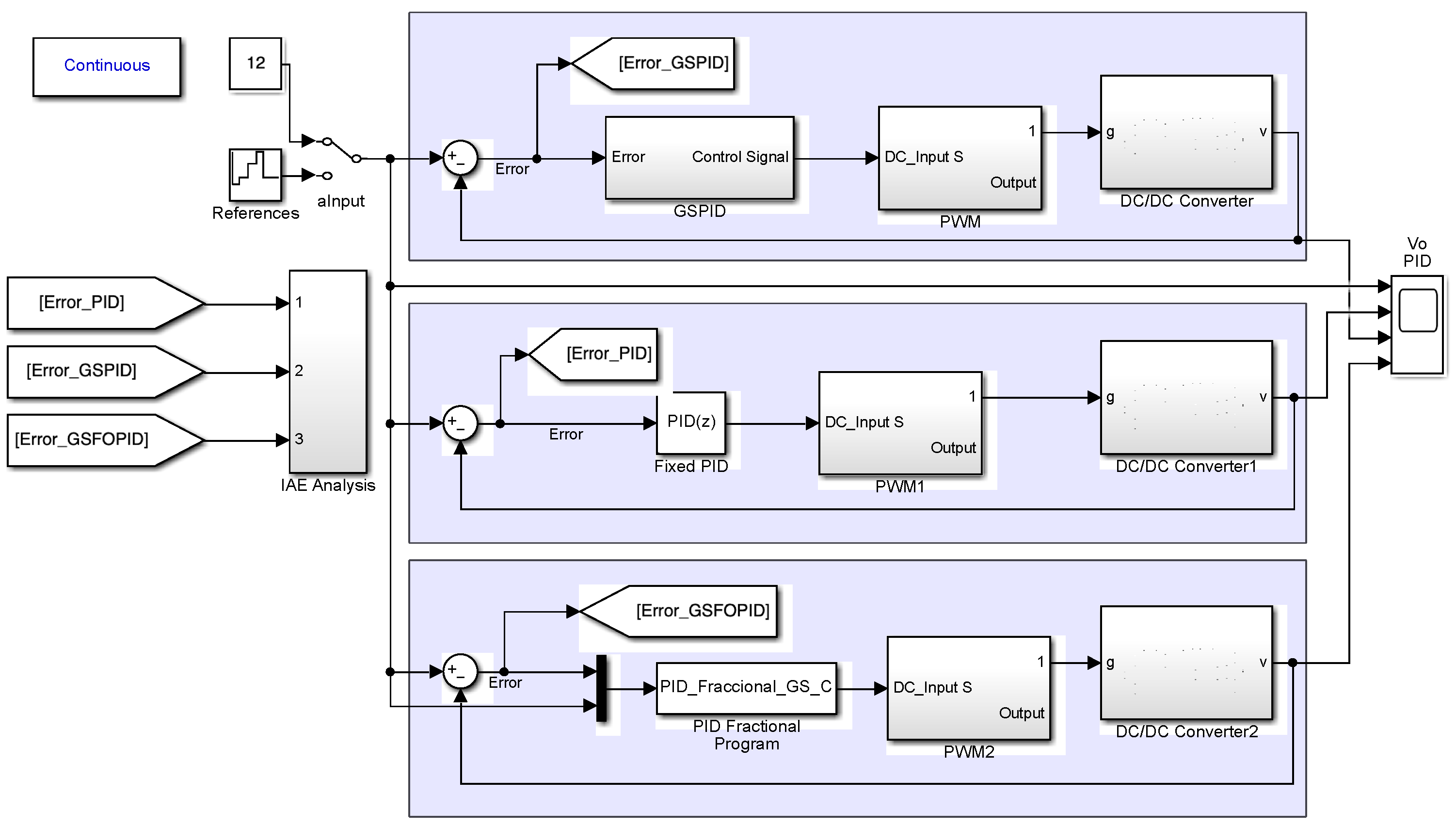
4.3.1. Simulation Overview

To evaluate the controllers, a Simulink^© platform was developed (Figure 3). The figure is divided into three closed loops, each of them with a different type of control applied to the designed DC–DC quadratic converter. As can be seen, the input signal and reference can be selected as fixed or variable, depending on the type of study desired. The top block shows the GS-PID control, while the fixed PID control is shown in the middle loop. On the other hand, the GS-FO-PID control is shown in the lower loop. The GS-PID is devolved using directly Simulink^© 2024b blocks, but the GS-FO-PID has been developed using an S function. Both algorithms use the reference as the factor to change the values of the parameters of the controllers. Figure 3 also shows the block where the analysis of the error integral is performed, in this case, using the IAE criterion.

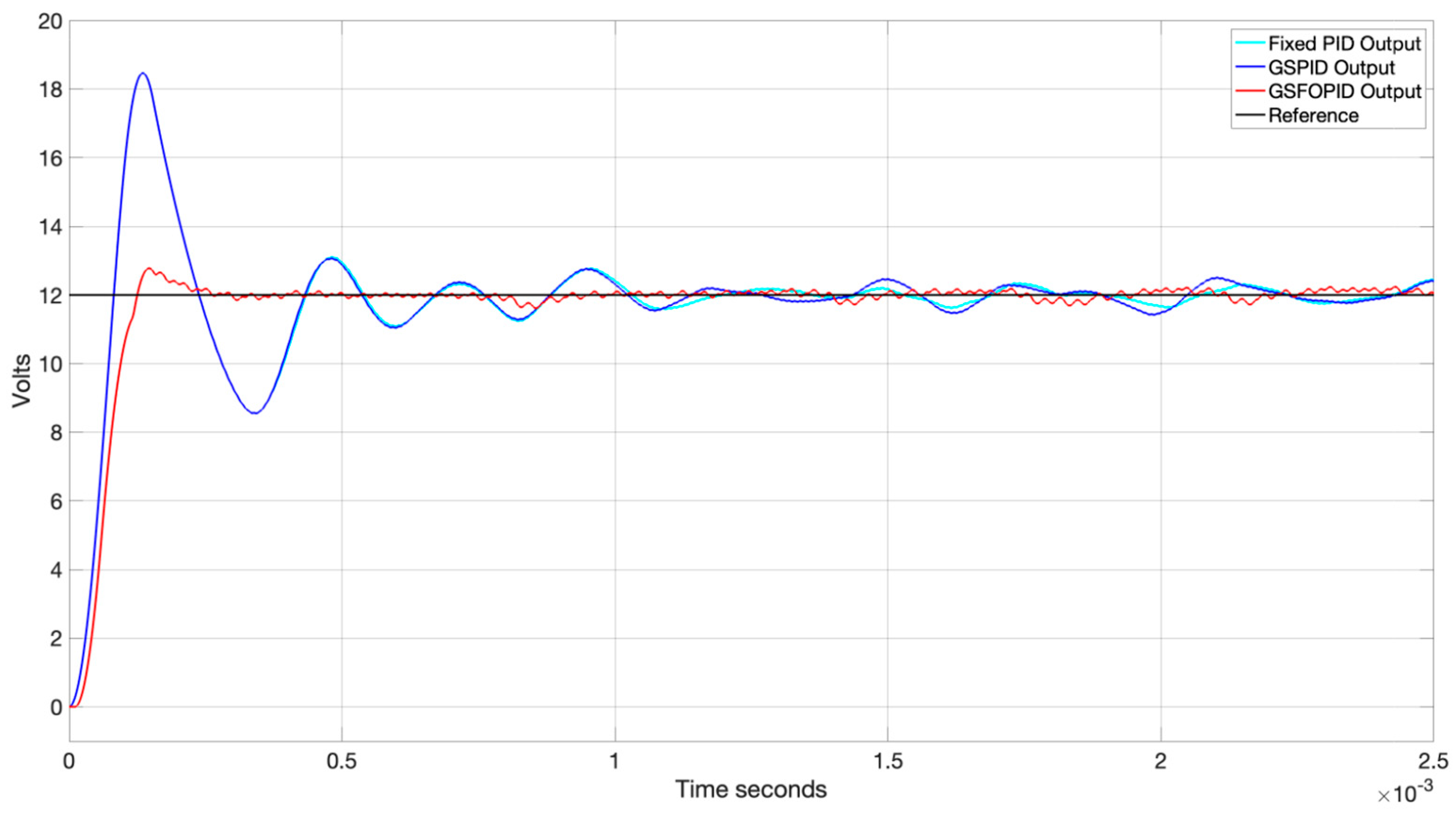
4.3.2. Scenario 1: Reference Voltage Change

To show the performance of the controllers, voltage changes were simulated, starting at 5 V, then going to 12 V, from there to 24 V, and finally 36 V. Changes were made every 0.0025 s; see Figure 4.

Figure 5 shows in detail the response of the system to changes in the reference voltage. In Figure 5a, the reference voltage is 5 volts. A decrease in overshooting by 40% can be observed when the converter is controlled by GS-FO-PID compared with the response with fixed PID and GS-PID controls, as well as the ripple at steady-state output being greatly reduced under GS-FO-PID control. Figure 5b–d shows the system with voltage references of 12, 24, and 36 volts, respectively. As can be seen, in all these cases, overshooting is practically zero when the system is controlled by GS-FO-PID, while the curve in the state stable is also reduced. However, this increases when the voltage reference is 36 Volts (Figure 5a). However, this amplitude is not higher than the other two controls evaluated. From the above, it can be said that in all cases, an improvement in the substantial reduction in the maximum overshoot is noted when the QBC is regulated by the GS-FO-PID controller.

Table 4. Overshooting of the quadratic buck converter under the controllers.

Voltage	Fixed PID	GS-PID	GS-FO-PID
5 V	50%	50%	20%
12 V	50%	50%	0%
24 V	65%	68%	0%
36 V	70%	50%	1%

summarizes these results. On the other hand, the stabilization time remains practically constant with all controllers. This is because the ripple present at the output—something expected in switched systems—does not allow accurate measurement of this parameter. However, a reduction in the amplitude of the ripple is reduced when the QBC is driven by GS-FO-PID.

It is expected that the behavior of the quadratic buck converter at 12 V would be the same for a fixed PID as for GS-PID; however, it must be considered that the initial conditions are not the same. By performing a simulation with both circuits starting at zero and uncharged reactive elements, a fairly similar behavior is obtained with both controllers (fixed PID and GS-PID; see Figure 6).

In order to measure the improvement in the operation of the quadratic buck converter under the GS-FO-PID controller, an analysis of the error integral was performed. Since an optimal system based on this criterion is a system that has reasonable damping and a satisfactory transient response, an IAE analysis was selected [46]. It was found that in all operational cases, the GS-FO-PID showed a lower value of this index; see

Table 5. IAE of the controllers.

Voltage	Fixed PID	GS-PID	GS-FO-PID
5 V	0.8673 × 10−3	0.8686 × 10−3	0.5886 × 10−3
12 V	1.356 × 10−3	1.448 × 10−3	0.7999 × 10−3
24 V	2.895 × 10−3	2.972 × 10−3	2.059 × 10−3
36 V	3.056 × 10−3	2.484 × 10−3	2.207 × 10−3

.

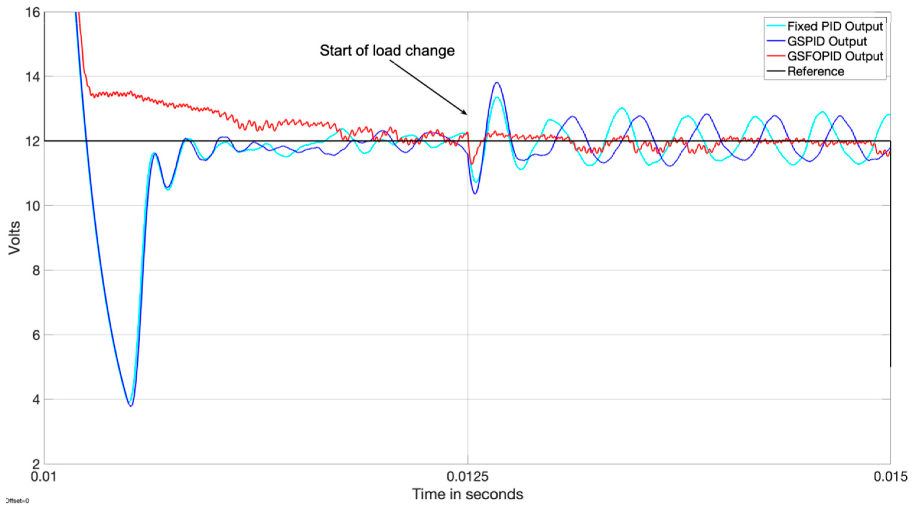
4.3.3. Scenario 2: Load Change

To verify that the output voltage remains within the regulation limits, a load shift test was performed. Therefore, when the system was operating at 12 V, a sudden change in load was caused at 0.0125 s of simulation, from 5 to 2.5 ohms, which generated an increase in the output ratio in all controllers. However, as can be seen in Figure 7, after an increase in the amplitude of the oscillation, the system returned to a ripple response. In the case of GS-FO-PID, the amplitude value of the ripple almost has no variation. This shows that the system controlled under GS-FO-PID has a better response to changes in load, even in the case evaluated, which was 50%.

The results of the simulations shown in this section corroborate that the GS-FO-PID controller improves the system’s response by reducing overshoots when the system is subject to reference changes. Also, the response to changes in load is improved when the system is controlled with the GS-FO-PID controller compared with the other controls evaluated. This means that the GS-FO-PID improves the dynamic response of the quadratic buck converter to both reference changes and load changes.

5. Conclusions

This paper has shown the effectiveness of a gain scheduling fractional order PID controller driving a quadratic buck converter improving the dynamic response. The simulation results have shown how GS-FO-PID can be applied to a quadratic buck converter to improve its performance, which is possible because GS-FO-PID considers the nonlinear nature of the converter, improving the direct transient responses. In particular, selecting different values of FO-PID parameters depending on the value of the input voltage and the reference allows the GS-FO-PID to produce a good response within each operational case, reducing overshooting. Additionally, it assumes load changes in a good way. As a perspective of this work, further study to determine the operating ranges for each set of GS-FO-PID parameters is necessary. The way in which the parameters for the GS-FO-PID are chosen could be improved by employing autonomous learning strategies, machine learning, and deep learning. Similarly, it is necessary to carry out an exhaustive study on the stability of the regulated system with the controller proposed in this work. The application of this type of control to other power converters, such as the boost and buck–boost, should also be evaluated. In general, these promising results allow and encourage the belief that GS-FO-PID could yield tangible benefits for the operation of DC–DC quadratic converters.

References

1. Okati, M.; Eslami, M.; Shahbaz, M.J. A New Transformerless DC/DC Converter with Dual Operating Modes and Continuous Input Current Port. IET Gener. Transm. Distrib. 2023, 17, 1553–1567. [Google Scholar] [CrossRef]
2. Okati, M.; Eslami, M.; Shahbazzadeh, M.J. A Non-Isolated DC-DC Converter with Dual Working Modes and Positive Output Voltage. Electr. Power Compon. Syst. 2021, 49, 1143–1157. [Google Scholar] [CrossRef]
3. Okati, M.; Eslami, M.M.; Jafari Shahbazzadeh, M.; Shareef, H. A New Transformerless Quadratic Buck-Boost Converter with High Voltage Gain Ratio and Continuous Input/Output Current Port. IET Power Electron. 2022, 15, 1280–1294. [Google Scholar] [CrossRef]
4. Damodaran, R.V.; Shareef, H.; Errouissi, R.; Eslami, M. A Common Ground Four Quadrant Buck Converter for DC-AC Conversion. IEEE Access 2022, 10, 44855–44868. [Google Scholar] [CrossRef]
5. Pandey, K.; Kumar, M.; Kumari, A.; Kumar, J. Control of Quadratic Buck Converter Using Non-Linear Controller. In Proceedings of the IEEE 17th India Council International Conference (INDICON), New Delhi, India, 11–13 December 2020. [Google Scholar] [CrossRef]
6. Arteaga-Orozco, M.I. Nonlinear Control of Switched DC/DC Converters: Performance Analysis and Experimental Verification. Ph.D. Thesis, UPC, Institut d’Organització i Control de Sistemes Industrials, Barcelona, Spain, 2007. [Google Scholar] [CrossRef]
7. Ali, M.S.; Soliman, M.; Hussein, A.M. Robust Controller of Buck Converter Feeding Constant Power Load. J. Control Autom. Electr. Syst. 2021, 32, 153–164. [Google Scholar] [CrossRef]
8. Trakuldit, S.; Tattiwong, K.; Bunlaksananusorn, C. Design and evaluation of a Quadratic Buck Converter. In Proceedings of the 8th International Conference on Power and Energy Systems Engineering (CPESE 2021), Fukuoka, Japan, 10–12 September 2021. [Google Scholar]
9. Carbajal-Gutierrez, E.E.; Morales-Saldana, J.A.; Leyva-Ramos, J. Modeling of a Single-Switch Quadratic Buck Converter. IEEE Trans. Aerosp. Electron. Syst. 2005, 41, 1451–1457. [Google Scholar] [CrossRef]
10. Ortiz-Lopez, M.; Leyva-Ramos, J.; Carbajal-Gutierrez, E.E.; Morales-Saldana, J.A. Modelling and analysis of switch-mode cascade converters with a single active switch. IET Power Electron. 2008, 1, 478–487. [Google Scholar] [CrossRef]
11. Ayachit, A.; Kazimierczuk, M.K. Steady-state analysis of PWM quadratic buck converter in CCM. In Proceedings of the IEEE 56th International Midwest Symposium on Circuits and Systems (MWSCAS), Columbus, OH, USA, 4–7 August 2013. [Google Scholar]
12. Mostaan, A.; Gorji, S.A.; Soltani, M.; Ektesabi, M. A novel quadratic buck-boost DC-DC converter without floating gate-driver. In Proceedings of the 2nd Annual Southern Power Electronics Conference (SPEC), Auckland, New Zealand, 5–8 December 2016. [Google Scholar] [CrossRef]
13. Bonela, A.K.; Sarkar, M.K.; Kumar, K. Robust non-fragile control of DC–DC buck converter. Electr. Eng. 2024, 106, 983–991. [Google Scholar] [CrossRef]
14. Montano-Saavedra, A.C.; Barra-Junior, W.; de Medeiros, R.L.P.; Roozembergh-Junior, C.; Sovano-Gomes, A. Experimental Evaluation of the Robust Controllers Applied on a Single Inductor Multiple Output DC-DC Buck Converter to Minimize Cross Regulation Considering Parametric Uncertainties and CPL Power Variations. Energies 2024, 17, 3359. [Google Scholar] [CrossRef]
15. Kumari, S.; Rayguru, M.M.; Upadhyaya, S. Analysis of Model Predictive Controller versus Linear Quadratic Regulator for DC-DC Buck Converter Systems. In Proceedings of the IEEE International Conference on Intelligent Computing and Control Systems, Madurai, India, 17–19 May 2023. [Google Scholar]
16. Raza, M.M.; Rayguru, M.M.; Kaushik, G. Robust Model Predictive Control of a Buck Converter with Constraints. In Proceedings of the International Conference on Computational Intelligence and Sustainable Engineering Solutions (CISES), New Delhi, India, 28–30 April 2023. [Google Scholar]
17. Fetene, Y.; Ayenew, E.; Feleke, S. Full state observer-based pole placement controller for pulse width modulation switched mode voltage-controlled buck Converter. Heliyon 2024, 10, e30662. [Google Scholar] [CrossRef] [PubMed]
18. Nanyan, N.F.; Ahmad, M.A.; Hekimoglu, B. Optimal PID controller for the DC-DC buck converter using the improved sine cosine algorithm. Results Control. Optim. 2024, 14, 100352. [Google Scholar] [CrossRef]
19. Bui, V.-H.; Mohammadi, S.; Das, S.; Hussain, A.; Hollweg, G.V.; Su, W. A critical review of safe reinforcement learning strategies in power and energy systems. Eng. Appl. Artif. Intell. 2025, 143, 110091. [Google Scholar] [CrossRef]
20. Lopez-Santos, O.; Flores-Bahamonde, F.; Torres-Pinzon, C.A.; Haroun, R.; Valderrama-Blavi, H.; Garriga, J.A.; Martınez-Salamero, L. Multi-loop Sliding-Mode Control for a Battery Charger Using a Quadratic Buck Converter. In Proceedings of the IEEE 8th Southern Power Electronics Conference (SPEC), Florianopolis, Brazil, 4–6 December 2023. [Google Scholar]
21. Pop, G.M.; Pop-Calimanu, I.M.; Lascu, D. Fourth-Order Quadratic Buck Converter Controller Design. Sensors 2024, 24, 557. [Google Scholar] [CrossRef] [PubMed]
22. Acosta-Rodriguez, R.A.; Martinez-Sarmiento, F.H.; Munoz-Hernandez, G.A.; Portilla-Flores, E.A.; Salcedo-Parra, O.J. Validation of Passivity-Based Control and Array PID in High-Power Quadratic Buck Converter Through Rapid Prototyping. IEEE Access 2024, 12, 58288–58316. [Google Scholar] [CrossRef]
23. Karaket, K.; Bunlaksananusorn, C. Modeling of a Quadratic Buck Converter. In Proceedings of the 8th Electrical Engineering/Electronics, Computer, Telecommunications and Information Technology (ECTI), Khon Kaen, Thailand, 17–19 May 2011. [Google Scholar]
24. Ogata, K. Ingeniería de Control Moderna, 5th ed.; Pearson Education: Madrid, Spain, 2010. (In Spanish) [Google Scholar]
25. Orelind, G.; Wozniak, L.; Medanic, J.; Whitemore, T. Optimal PID gain schedule for Hydrogenerators-Design and application. IEEE Trans. Energy Convers. 1989, 4, 300–307. [Google Scholar] [CrossRef]
26. Petras, I. Fractional Calculus and Applied Analyisis. Int. J. Theory Appl. 2012, 15, 282–303. [Google Scholar]
27. Caputo, M. Linear Models of Dissipation whose Q is almost Frequency Independent -I. Geophys. J. R. Astron. Soc. 1967, 13, 529–539. [Google Scholar] [CrossRef]
28. Podlubny, I. Fractional Differential Equations; Academic Press: San Diego, CA, USA, 1999. [Google Scholar]
29. Monje, C.A.; Chen, Y.; Vinagre, B.M.; Xue, D.; Feliu, V. Fractional Order Systems and Controls: Fundamentals and Applications; Johnson, Ed.; Springer-Verlag: London, UK, 2010; p. 414. [Google Scholar]
30. Podlubny, I.; Dorcak, L.; Kostial, I. On Fractional Derivatives, Fractional-Order Dynamic Systems and PIlDu Controllers. In Proceedings of the Conference on Decision and Control, San Diego, CA, USA, 10–12 December 1997. [Google Scholar]
31. Podlubny, I. Fractional-Order Systems and PILDu-Controllers. IEEE Trans. Autom. Control 1999, 44, 208–214. [Google Scholar] [CrossRef]
32. Vinagre, B.M.; Podlubny, I.; Dorcak, L.; Feliu, V. On Fractional PID Controllers: A Frequency Domain Aproach. In Proceedings of the IFAC Digital Control: Past, Present and Future of PID Control, Terrassa, Spain, 5–7 April 2000. [Google Scholar]
33. Monje, C.A.; Vinagre, B.M.; Feliu, V.; Chen, Y.Q. On Auto-Tuning of Fractional Order PIlDu Controllers. In Proceedings of the 2nd IFAB Workshop on Fractional Differentiation and its Applications, Porto, Portugal, 19–21 July 2006. [Google Scholar]
34. Monje, C.A.; Vinagre, B.M.; Feliu, V.; Chen, Y.Q. Tuning and auto-tuning of fractional order controllers for industry applications. Control. Eng. Pract. 2008, 16, 798–812. [Google Scholar] [CrossRef]
35. Petras, I. Tuning and implementation methods for fractional-order controllers. Fract. Calc. Appl. Anal. 2012, 15, 282–303. [Google Scholar] [CrossRef]
36. Milanesi, M.; Padula, F.; Visioli, A. On the implementation of gain scheduling in FOPID controllers. IFAC Pap. Online 2024, 58, 330–335. [Google Scholar] [CrossRef]
37. Ayere-Junior, F.A.C.; Bessa, I.; Batista-Pereira, V.M.; Da Silva-Farias, N.J.; de Menezes, A.R.; de Medeiros, R.L.P.; Chavez-Filho, J.E.; Lenzi, M.K.; Da Costa-Junior, C.T. Fractional Order Pole Placement for a buck converter based on commensurable transfer function. ISA Trans. 2020, 107, 370–384. [Google Scholar]
38. Wu, Z.; Li, D.; Xue, Y.; He, T.; Zheng, S. Tuning for Fractional Order PID Controller based on Probabilistic Robustness. IFAC Pap. Online 2018, 51, 675–680. [Google Scholar] [CrossRef]
39. Awouda, A.E.A.; Mamat, R.B. Refine PID tuning rule using ITAE criteria. In Proceedings of the 2010 2nd International Conference on Computer and Automation Engineering (ICCAE), Singapore, 26–28 February 2010. [Google Scholar]
40. Chen, Y.Q.; Petras, I.; Xue, D. Fractional Order Control—A Tutorial. In Proceedings of the 2009 American Control Conference, St. Louis, MO, USA, 10–12 June 2009. [Google Scholar]
41. Choudhary, S.K. Stability and Performance Analysis of Fractional Order Control Systems. WSEAS Trans. Syst. Control 2014, 9, 438–444. [Google Scholar]
42. Dewangan, P.D.; Singh, V.P.; Sinha, S.L. Design of FOPID controller for higher order continuous interval system using improved approximation ensuring stability. SN Appl. Sci. 2021, 3, 493. [Google Scholar] [CrossRef]
43. Rhouma, A.; Hafsi, S.; Laabidi, K. Stabilizing and Robust Fractional PID Controller Synthesis for Uncertain First-Order plus Time-Delay Systems. Math. Probl. Eng. Hindawi 2021, 2021, 9940634. [Google Scholar] [CrossRef]
44. Matignon, D. Generalized Fractional Differential and Difference Equations: Stability Properties and Modelling Issues. In Proceedings of the Mathematical Theory of Networks and Systems Symposium, Padova, Italy, 6–10 July 1998. [Google Scholar]
45. Astrom, K.J.; Wittenmark, B. Adaptive Control; Addison-Wesley: Reading, MA, USA, 1989. [Google Scholar]
46. Sangeetha, S.; Revathi, B.S.; Balamurugan, K.; Suresh, G. Performance analysis of buck converter with fractional PID controller using hybrid technique. Robot. Auton. Syst. 2023, 169, 104515. [Google Scholar] [CrossRef]
Figure 1. Quadratic buck converter. (a) ON state. (b) OFF state.
Fractalfract 09 00160 g001
Figure 2. Schematic diagram of the GS-PID controller.
Fractalfract 09 00160 g002
Figure 3. Simulink© models used to evaluate the controllers.
Fractalfract 09 00160 g003
Figure 4. Outputs of the quadratic buck converter under different controllers.
Fractalfract 09 00160 g004
Figure 5. Details of the outputs of the quadratic buck converter under different controllers with voltage change.
Fractalfract 09 00160 g005aFractalfract 09 00160 g005b
Figure 6. Outputs of the quadratic buck converter under different controllers with voltage change with the initial conditions equal to zero.
Fractalfract 09 00160 g006
Figure 7. Response of the quadratic buck converter with a load change.
Fractalfract 09 00160 g007