A Compact Difference-Galerkin Spectral Method of the Fourth-Order Equation with a Time-Fractional Derivative

Abstract

In this article, we proposed a compact difference-Galerkin spectral method for the fourth-order equation in multi-dimensional space with the time-fractional derivative order $\alpha \in (1,2)$. The novel compact difference-Galerkin spectral method can effectively address the issue of high-order derivative accuracy and handle complex boundary problems. Simultaneously, the main conclusions of this article, including the stability, convergence, and solvability of the method, are derived. Finally, some computational experiments are illustrated to demonstrate the superiority of the compact difference-Galerkin spectral method.

1. Introduction

Fractional calculus is generally the generalization of integer-order derivatives and integrals to the case of arbitrary non-integer orders. However, the concept of fractional calculus emerged almost simultaneously with integer-order calculus. The concept of fractional calculus was first proposed by L’Hospital and Leibniz [1]. Historically, Leibniz, Euler, Laplace, Lacroix, and Fourier all noticed derivatives of arbitrary orders. A series of articles published by Liouville from 1832 to 1837 made him the de facto founder of the theory of fractional calculus. After Liouville, Riemann, Fourier, Willian Center, Morgan, Bernhard Riemann, Cayley, and Weyl also conducted work of great significance. After more than 300 years of development, fractional calculus and fractional differential equations have been deeply studied and widely applied in many fields of science and engineering, including fluid mechanics, electronic networks, electromagnetics, probability theory, statistics, viscoelasticity theory, electrochemistry, quantum mechanics, plasma physics, superconductivity, materials science, turbulence, economics and finance, etc. [2,3,4,5,6,7,8,9].

In 1965, Professor Mandelbrot of Yale University in the United States proposed the concept of fractals and believed that there are a large number of phenomena with fractional dimensions in nature and engineering, and their essence is the self-similarity between the whole and the part [10]. It is believed that there is a close internal connection between fractional Brownian motion and the definition of fractional calculus proposed by Riemann-Liouville. Since then, as the basis of fractal geometry and fractal dynamics, the research on fractional operator theory and fractional differential equations has begun to receive extensive attention, and the focus of fractional calculus research has gradually shifted from the pure mathematical field to other disciplinary fields.

Geophysicists Caputo [11] and Mainardi [12] used the fractional calculus method to study complex viscoelastic and rheological media and developed several new mechanical models. Moreover, more importantly, Caputo [11] developed a new definition different from the traditional Riemann-Liouville fractional-derivative definition, which overcame the strong singularity of the former and naturally included the initial conditions in the definition, and has been widely applied in solving practical problems. The first doctoral dissertation on fractional-order viscoelastic material modeling was completed by Bagley under the guidance of Torvik [13]. After that, the application of fractional calculus to the modeling of viscoelastic materials and other complex mechanical processes began to receive increasing attention.

Here, we will consider the following fourth-order equation with a time-fractional derivative in multi-dimensional space:

$$\begin{array}{cc}\hfill & {}_0{}^c\mathfrak{D}_t^{\alpha }u(\mathbf{x},t)-{}_0{}^c\mathfrak{D}_t^{\alpha }\mathrm{\Delta }u(\mathbf{x},t)=-{▵}^{2}u(\mathbf{x},t)+▵u(\mathbf{x},t)+f(\mathbf{x},t),\mathbf{x}\in \mathrm{\Omega },t\in (0,T],\hfill \end{array}$$

(1)

with the following initial and boundary conditions:

$$\begin{array}{cc}\hfill & u(\mathbf{x},0)=u_0\left(\mathbf{x}\right),u_t(\mathbf{x},0)=v_0\left(\mathbf{x}\right),\mathbf{x}\in \mathrm{\Omega },\hfill \\ \hfill & u(\mathbf{x},t)=\mathrm{\Delta }u(\mathbf{x},t)=0,\mathbf{x}\in \mathrm{\Gamma },t\in (0,T],\hfill \end{array}$$

(2)

where $u(\mathbf{x},t)$ is an unknown function and $f(\mathbf{x},t)$ is the source term. Here, ${}_0{}^c\mathfrak{D}_t^{\beta }$ denotes the Caputo fractional derivative of order $\beta$ and it is defined by [2,11,12]

$$\begin{array}{cc}\hfill & {}_0{}^c\mathfrak{D}_t^{\beta }u(\mathbf{x},t)={\displaystyle \frac{1}{\mathrm{\Gamma }(2-\beta )}}{\int }_0^t{\displaystyle \frac{{\partial }^{2}u(\mathbf{x},\eta )}{\partial {\eta }^2}}{\displaystyle \frac{d\eta }{{(t-\eta )}^{\beta -1}}},1\le \beta \le 2,\hfill \end{array}$$

(3)

where $\mathrm{\Gamma }(·)$ is the Gamma function.

In recent decades, the fourth-order model system [14,15] constitutes a significant element of the fractional-order system. It is widely present in diverse domains such as physics, engineering, and statistics. For instance, it can be found in wave equations of beam systems [16], a system of flat surface furnished with grooves [17,18], and several formations in mathematical modeling pertaining to fourth-order subdiffusion systems [18,19,20,21], among others. Owing to the circumstance that most fractional partial differential equations lack an analytical solution, a substantial number of researchers have focused their efforts on approximation or numerical techniques applicable to these fractional-order systems. A significant portion of the research community has centered on the strong format. This particular model is directly derived from the original discrete equation and is thus also known as the collocation method. The strong formulation proves to be reliable, exhibits a simple structure, and expedites the establishment of the algebraic system. The homotopy analysis method has been employed to obtain approximations for specific fractional partial differential equations, as reported in relevant references [22,23]. A finite difference approximation in the time direction and a finite element method in the spatial direction are presented and deliberated to seek the numerical solutions of a time-fractional fourth-order reaction–diffusion problem. Furthermore, certain fractional differential equations which are applied in the modeling of dynamical systems have been explored by means of an implicit difference format, as documented in reference [24]. Parvizi et al. have effectively harnessed the Jacobi collocation method in reference [25] to acquire the numerical resolution of the fractional equation accompanied by a nonlinear source term, and comparable research undertakings are still in progress.

Nearly all of these schemes need to take into account the strong form (collocation method). In the strong form, it demands that the analytic function possesses a relatively high degree of smoothness. Meanwhile, the Galerkin weak form is more convenient for dealing with complex boundary conditions. For complex geometric shapes and boundary conditions, the strong form may lead to great difficulties in solving the equations. The Galerkin weak form is capable of handling boundary conditions more flexibly. Meanwhile, this article employs the time derivative scenario of the unknown function as it is convenient for obtaining the representations of the second-order derivative situation and facilitating the integration process. By combining the advantages mentioned above, the new scheme we obtain is more stable. The remainder of this paper is structured in the following manner: In Section 2 and Section 3, a compact difference-Galerkin method is deduced and several preliminary concepts as well as lemmas are introduced. In Section 4, the principal conclusions of this article, which encompass the stability, convergence, and solvability of the method, are verified. In Section 5, a number of computational experiments are exemplified to exhibit the superiority of the difference-Galerkin method. Eventually, certain conclusions are provided in Section 6.

2. Algebraic Equation and Preliminaries

2.1. Variational Equations for the Fourth-Order Equation

Denote the inner product as follows:

$$\begin{array}{cc}\hfill & (u,w)={\int }_{\mathrm{\Omega }}uwd\mathrm{\Omega },\forall u,w\in L^2\left(\mathrm{\Omega }\right).\hfill \end{array}$$

(4)

Then, the variable formulation of (1) is restated in the following manner:

$$\begin{array}{cc}\hfill & ({}_0{}^c\mathfrak{D}_t^{\alpha }u,w)+({}_0{}^c\mathfrak{D}_t^{\alpha }\nabla u,\nabla w)=(\nabla (▵u),\nabla w)-(\nabla u,\nabla w)+(f,w),\forall w\in H^1\left(\mathrm{\Omega }\right).\hfill \end{array}$$

(5)

Let $\left\{t_n\right|n\ge 0\}$ denote the equidistant time interval, with $t_n=n\tau ,\tau >0$. Moreover, suppose

$$\begin{array}{cc}\hfill & \partial v\left(t_{i+1}\right)/\partial t=(v^{i+1}-v^i)/\tau ,u^n=u^0+\tau \sum _{k=1}^n(v^{k-1}+v^k)/2,\hfill \end{array}$$

(6)

where $u^n,v^n$ represent the values of the function and its first derivative function at the time $t_n$.

The difference scheme of (1) and (5) is presented as follows:

$$\begin{array}{cc}\hfill & {\displaystyle \frac{1}{\tau \mathrm{\Gamma }(2-\alpha )}}\left(\left[a_0{v}^n-\sum _{k=1}^{n-1}(a_{n-k-1}-a_{n-k})v^n-a_{n-1}{v}_0\right],w\right)\hfill \\ \hfill & +{\displaystyle \frac{1}{\tau \mathrm{\Gamma }(2-\alpha )}}\left(\nabla \left[a_0{v}^n-\sum _{k=1}^{n-1}(a_{n-k-1}-a_{n-k})v^n-a_{n-1}{v}_0\right],\nabla w\right)\hfill \\ \hfill & =\left(\nabla \left(\mathrm{\Delta }\left(u^{n-1}+\tau {\displaystyle \frac{v^{n-1}+v^n}{2}}\right)\right),\nabla w\right)-\left(\nabla \left(u^{n-1}+\tau {\displaystyle \frac{v^{n-1}+v^n}{2}}\right),\nabla w\right)\hfill \\ \hfill & +(f^n,w)+(R_{\tau }^n,w),w\in H_0^1\left(\mathrm{\Omega }\right),\hfill \end{array}$$

(7)

where $a_l={\int }_{t_l}^{t_{l+1}}{\displaystyle \frac{dt}{t^{\alpha -1}}}={\displaystyle \frac{{\tau }^{3-\alpha }}{2-\alpha }}\left[{(l+1)}^{2-\alpha }-l^{2-\alpha }\right],b_l=a_{n-l}$. It is easy to verify that $a_l$ is a monotone decreasing sequence for each n with $a_0={\tau }^{2-\alpha }/(2-\alpha )$.

2.2. Galerkin–Legendre Scheme

Let ${\left\{L_i\right\}}_{j=0}^p$ be a set of orthogonal Legendre polynomial bases in one-dimensional space:

$$L_0=1,L_1=x,(j+2)L_{j+2}=(2j+3)x{L}_{j+1}-(j+1)L_j,j=2,\cdots$$

such that

$$(L_i,L_j)={(i+1/2)}^{-1}{\delta }_{ij},0\le i,j<\infty .$$

Here, $\delta$ represents the delta function. From [26], two kinds of the best basis functions in $H_0^1\left(\mathrm{\Omega }\right)$ and $H_0^2\left(\mathrm{\Omega }\right)$ are

$$H_0^1\left(\mathrm{\Omega }\right)=span\{{\varphi }_i\left(x\right),0\le i<\infty \},H_0^2\left(\mathrm{\Omega }\right)=span\{{\psi }_i\left(x\right),0\le i<\infty \},$$

where

$${\varphi }_i\left(x\right)=L_i\left(x\right)-L_{i+2}\left(x\right),{\psi }_i\left(x\right)=L_i\left(x\right)-{\displaystyle \frac{2(2i+5)}{2i+7}}{L}_{i+2}\left(x\right)+{\displaystyle \frac{2i+3}{2i+7}}{L}_{i+4}\left(x\right),i=0,1,\cdots$$

such that

$$({\varphi }_i^{\prime },{\varphi }_j^{\prime })={(4i+6)}^{-1}{\delta }_{ij},({\psi }_i^{″},{\psi }_j^{″})={\left(2{(2i+3)}^2(2i+5)\right)}^{-1}{\delta }_{ij},0\le i,j<\infty .$$

2.3. Algebraic Equation of Weak Form with the Boundary Conditions

Take a one-dimensional problem as an example, assuming a column vector

$$\begin{array}{cc}\hfill & \mathbf{U}={[u_0,u_1,u_2,\cdots ,u_M]}^T,\mathbf{V}={[v_0,v_1,v_2,\cdots ,v_M]}^T,\hfill \end{array}$$

(8)

where $u\left(x_i\right),v\left(x_i\right),and w\left(x_i\right)$ represent the i-st node function value, derivative value of u, and w function value, respectively, and M represents the number of nodes.

Using the spectral method, the r-th derivative of U can be discretized as

$$\begin{array}{cc}\hfill & {\mathbf{U}}^{\left(r\right)}={\mathbf{A}}^r\mathbf{U},\hfill \end{array}$$

(9)

where $\mathbf{A}$ is the first-order differential matrix.

In general, we also have

$$\begin{array}{cc}\hfill & {\int }_{\mathrm{\Omega }}g\left(\mathbf{x}\right)d\left(\mathrm{\Omega }\right)=\sum _{i=1}^{M}g\left({\mathbf{x}}_i\right){\omega }_i.\hfill \end{array}$$

(10)

${\omega }_i$ is called the volume element on the node ${\mathbf{x}}_i$ in physics, and it is also named the weight for the corresponding numerical integration in mathematics.

To facilitate the application of boundary conditions, the variables $v^n$ and $\mathrm{\Delta }{u}^n$ are used simultaneously with the following supplementary equation:

$$\begin{array}{cc}\hfill & \left(\mathrm{\Delta }{u}^n,w\right)+\left(\nabla \left(u^{n-1}+\tau {\displaystyle \frac{v^{n-1}+v^n}{2}}\right),\nabla w\right)=0.\hfill \end{array}$$

(11)

We multiply both sides of the above equation by $-{\displaystyle \frac{2}{\tau }}$ and considering the arbitrariness of w, and we use Equations (7) and (11) to obtain the following system of equations in matrix form:

$$\begin{array}{c}\hfill \left[\begin{array}{cc}{\displaystyle \frac{a_0}{\tau \mathrm{\Gamma }(2-\alpha )}}(\mathbf{\Omega }+{\mathbf{A}}^{\mathbf{T}}\mathrm{\Omega }\mathbf{A})+{\displaystyle \frac{\tau }{2}}{\mathbf{A}}^{\mathbf{T}}\mathrm{\Omega }\mathbf{A}& -{\mathbf{A}}^{\mathbf{T}}\mathrm{\Omega }\mathbf{A}\\ -{\mathbf{A}}^{\mathbf{T}}\mathbf{\Omega }\mathbf{A}& -{\displaystyle \frac{2}{\tau }}\mathbf{\Omega }\end{array}\right]\left[\begin{array}{c}{\mathbf{V}}^{\mathbf{n}}\\ \mathbf{\Delta }{\mathbf{U}}^{\mathbf{n}}\end{array}\right]=\left[\begin{array}{c}\mathbf{P}\\ {\mathbf{A}}^{\mathbf{T}}\mathrm{\Omega }\mathbf{A}({\displaystyle \frac{2}{\tau }}{\mathbf{U}}^{n-1}+{\mathbf{V}}^{n-1})\end{array}\right],\end{array}$$

(12)

where $\mathbf{P}={\mathbf{P}}_{\mathbf{1}}+{\mathbf{P}}_{\mathbf{2}}+\mathrm{\Omega }\mathbf{F}$, ${\mathbf{P}}_{\mathbf{1}}={\displaystyle \frac{\mathbf{\Omega }(\mathbf{I}-\mathbf{\Delta })}{\tau \mathrm{\Gamma }(2-\alpha )}}\left[{\sum }_{k=1}^{n-1}(a_{n-k-1}-a_{n-k}){\mathbf{V}}^n+a_{n-1}{\mathbf{V}}_0\right]$, ${\mathbf{P}}_{\mathbf{2}}=\tau (\mathrm{\Omega }-{\mathbf{A}}^{\mathbf{T}}\mathrm{\Omega }\mathbf{A})\left(\mathbf{\Delta }{\mathbf{U}}^{n-1}+{\displaystyle \frac{\mathbf{\Delta }{\mathbf{V}}^{n-1}}{2}}\right)$, $\mathbf{\Omega }$ is a diagonal matrix composed of weight vectors ${\omega }_i$ and $\mathbf{F}$ is composed of the source terms of each node.

Further, we introduce the following boundary conditions: $\mathbf{B}{\mathbf{V}}^{\mathbf{n}}=-\mathbf{B}{\mathbf{V}}^{\mathbf{n}-\mathbf{1}}$, $\mathbf{B}\left(\mathbf{\Delta }{\mathbf{U}}^{\mathbf{n}}\right)=0$, where $\mathbf{B}$ is the matrix assembled from all boundary points.

2.4. Preliminary Lemmas

We also define

$$\begin{array}{cc}\hfill & {\parallel g^n\parallel }_{\infty }=\underset{0\le i\le M}{max}|g_i^n|,|\nabla g^n|=\sqrt{h\sum _{i=1}^M{\left(g_{i-1}^n\right)}^2},h=\prod _{x\in \mathbf{x}}{h}_x.\hfill \end{array}$$

(13)

Furthermore, in the case where $g\left(\mathrm{\Gamma }\right)=0$, we obtain

$$\begin{array}{cc}\hfill & {\parallel g^n\parallel }_{\infty }\le {\displaystyle \frac{\sqrt{D}}{2}}|\nabla g^n|,\hfill \end{array}$$

(14)

where D represents the measure of the spatial domain $\mathrm{\Omega }$.

Next, the following theorem offers an error estimation for the Galerkin method:

Theorem 1.

If u, w, $u_p$ and $w_p$$\in C^{n+1}\left(\mathrm{\Omega }\right)$, where Ω has a nonempty, open bounded set with a Lipschitz continuous boundary, then the following error estimates hold:

$${\parallel u^{\left(k\right)}-u_p^{\left(k\right)}\parallel }_{\infty }\le c_1{\parallel u^{n+1}\parallel }_{\infty }{h}^{min\{p,n+1\}-2-k},$$

and

$${\parallel (u^{\left(k_1\right)},w^{\left(k_2\right)})-\sum _{i=1}^{M}g\left({\mathbf{x}}_i\right)u_p^{\left(k_1\right)}{w}_p^{\left(k_2\right)}\parallel }_{\infty }\le c_1^{*}{h}^{2min\{p,n+1\}-4-k_1-k_2}.$$

For the high-dimensional case, the above corresponding properties also hold with a small change of the coefficient (see [26]).

3. Some Lemmas

Regarding the fractional derivative of the proposed scheme, upon setting w equal to v, some lemmas [27,28] are required:

Lemma 1.

For $n\ge 1$ and $t_k=k\tau$, $0\le k\le n$, we have

$$\begin{array}{cc}\hfill & 0\le \sum _{k=1}^n{\int }_{t_{k-1}}^{t_k}\left[{(t_n-t)}^{2-\alpha }-{\displaystyle \frac{{(t_{n-1}-t)}^{2-\alpha }+{(t_n-t)}^{2-\alpha }}{2}}\right]dt\le \left[{\displaystyle \frac{2-\alpha }{12}}+{\displaystyle \frac{2^{3-\alpha }}{3-\alpha }}-(1+2^{1-\alpha })\right]{\tau }^{3-\alpha }.\hfill \end{array}$$

(15)

Lemma 2.

Suppose $v\left(t\right)\in C^2\left([0,t_n]\right)$. Then,

$$\begin{array}{cc}\hfill & \left|{\int }_0^{t_n}{v}^{\prime }\left(t\right){\displaystyle \frac{dt}{{(t_n-t)}^{\alpha -1}}}-\sum _{k=1}^n{\displaystyle \frac{v^k-v^{k-1}}{\tau }}{\int }_{t_{k-1}}^{t_k}{\displaystyle \frac{dt}{{(t_n-t)}^{\alpha -1}}}\right|\hfill \\ \hfill & \le {\displaystyle \frac{{\tau }^{3-\alpha }}{2-\alpha }}\left[{\displaystyle \frac{2-\alpha }{12}}+{\displaystyle \frac{2^{3-\alpha }}{3-\alpha }}-(1+2^{1-\alpha })\right]{\parallel v\left(t\right)\parallel }_{L^{2,\infty }\left([0,t_n]\right)}.\hfill \end{array}$$

(16)

Lemma 3.

Suppose $v\left(t\right)\in C^2[0,t_n]$. Then,

$$\begin{array}{cc}\hfill & \left|{\int }_0^{t_n}{v}^{\prime }\left(t\right){\displaystyle \frac{dt}{{(t_n-t)}^{\alpha -1}}}-{\displaystyle \frac{1}{\tau }}\left[a_0{v}^n-\sum _{k=1}^{n-1}(a_{n-k-1}-a_{n-k})v^k-a_{n-1}{v}^0\right]\right|\hfill \\ \hfill & \le {\displaystyle \frac{{\tau }^{3-\alpha }}{2-\alpha }}\left[{\displaystyle \frac{2-\alpha }{12}}+{\displaystyle \frac{2^{3-\alpha }}{3-\alpha }}-(1+2^{1-\alpha })\right]{\parallel g\left(t\right)\parallel }_{L^{1,\infty }\left([0,t_n]\right)}.\hfill \end{array}$$

(17)

where $a_l^n$ is defined in (7) and $1<\alpha <2$.

Based on Lemma 3 and by introducing Equation (17), we have

$$\begin{array}{cc}\hfill {}^c\mathfrak{D}_0^{\alpha }u(x,t)& ={\displaystyle \frac{1}{\mathrm{\Gamma }(2-\alpha )}}{\int }_0^t{\displaystyle \frac{{\partial }^{2}u(x,t)}{\partial t^2}}{\displaystyle \frac{dt}{{(t_n-t)}^{\alpha -1}}},\hfill \\ \hfill & ={\displaystyle \frac{1}{\tau \mathrm{\Gamma }(2-\alpha )}}\left[a_0{v}^n-\sum _{k=1}^{n-1}(a_{n-k-1}-a_{n-k})v^k-a_{n-1}{v}^0\right]+{\left(r_1\right)}_i^n,\hfill \end{array}$$

(18)

and

$$\begin{array}{cc}\hfill & {\displaystyle \frac{\partial u_i^n}{\partial x}}=\sum _{i=1}^M{L}^{\prime }\left(x_i\right)u_i^n+{\left(r_2\right)}_i^n,{\displaystyle \frac{{\partial }^2{u}_i^n}{x^2}}=\sum _{i=1}^M{L}^{″}\left(x_i\right)u_i^n+{\left(r_3\right)}_i^n,\hfill \end{array}$$

(19)

where

$$\begin{array}{cc}\hfill & |{\left(r_1\right)}_i^n|\le c_1{\tau }^{3-\alpha },|{\left(r_2\right)}_i^n|\le c_2({\tau }^2+h^{min\{p,n+1\}-3}),|{\left(r_3\right)}_i^n|\le c_3({\tau }^2+h^{min\{p,n+1\}-4}).\hfill \end{array}$$

(20)

By substituting the aforesaid results into (1), taking into account the initial values and setting $w=v^n$, we obtain

$$\begin{array}{cc}\hfill & {\displaystyle \frac{1}{\tau \mathrm{\Gamma }(2-\alpha )}}\sum _i^M{\omega }_i{v}_i^n\left(a_0{v}_i^n-\sum _{k=1}^{n-1}(a_{n-k-1}-a_{n-k})v_i^k-a_{n-1}{v}_i^0\right)\hfill \\ \hfill & +{\displaystyle \frac{1}{\tau \mathrm{\Gamma }(2-\alpha )}}\sum _i^M{\omega }_i\nabla v_i^n\nabla \left(a_0{v}_i^n-\sum _{k=1}^{n-1}(a_{n-k-1}-a_{n-k})v_i^k-a_{n-1}{v}_i^0\right)\hfill \\ \hfill & =-\tau \sum _i^M{\omega }_i\mathrm{\Delta }(\sum _{k=1}^{n-1}{v}_i^k+{\displaystyle \frac{v_i^0+v_i^n}{2}})\mathrm{\Delta }{v}_i^n-\tau \sum _i^M{\omega }_i\nabla (\sum _{k=1}^{n-1}{v}_i^k+{\displaystyle \frac{v_i^0+v_i^n}{2}})\nabla v_i^n\hfill \\ \hfill & +\sum _i^M{\omega }_i{\widehat{F}}_i^n{u}_i+\left(R_i^n,v^n\right),\hfill \end{array}$$

(21)

where

$$\begin{array}{c}|R^n|\le C({\tau }^{3-\alpha }+h^{min\{p,n+1\}-4}).\hfill \end{array}$$

(22)

4. Main Results

Before proving the solvability, stability and convergence, we present the following lemmas:

Lemma 4.

For any $v=\{v\left(t_0\right),v\left(t_1\right),v\left(t_2\right),\cdots \}$, we have

$$\begin{array}{cc}\hfill & \sum _{n=1}^N\left(a_0^n{v}^n-\sum _{k=1}^{n-1}(a_{n-k-1}^n{v}^n-a_{n-k}^n{v}^n)v^k-a_{n-1}^n{v}^0,v^n\right)\ge {\displaystyle \frac{t_N^{1-\alpha }}{2}}\tau \sum _{n=1}^N\parallel v^n{\parallel }^2-{\displaystyle \frac{t_N^{2-\alpha }}{2(2-\alpha )}}{\parallel v^0\parallel }^2.\hfill \end{array}$$

(23)

Proof. 

$$\begin{array}{cc}\hfill & \sum _{n=1}^N\left(a_0^n{v}^n-\sum _{k=1}^{n-1}(a_{n-k-1}^n-a_{n-k}^n)v^k-a_{n-1}^n{v}^0,v^n\right)\hfill \\ \hfill & =\sum _{n=1}^N{a}_0^n{\parallel v^n\parallel }^2-\sum _{n=1}^N\sum _{k=1}^{n-1}(a_{n-k-1}^n-a_{n-k}^n)\left(v^k,v^n\right)-\sum _{n=1}^N{a}_{n-1}^n\left(v^0,v^n\right)\hfill \\ \hfill & \ge \sum _{n=1}^N{a}_0^n\parallel v^n{\parallel }^2-{\displaystyle \frac{1}{2}}\sum _{n=1}^N\sum _{k=1}^{n-1}(a_{n-k-1}^n-a_{n-k}^n)(\parallel v^k{\parallel }^2+\parallel v^n{\parallel }^2)-{\displaystyle \frac{1}{2}}\sum _{n=1}^N{a}_{n-1}^n(\parallel v^0{\parallel }^2+\parallel v^n{\parallel }^2)\hfill \\ \hfill & =\sum _{n=1}^N{a}_0^n\parallel v^n{\parallel }^2-{\displaystyle \frac{1}{2}}\sum _{n=1}^N\sum _{k=1}^{n-1}(a_{n-k-1}^n-a_{n-k}^n)\parallel v\left(t_k\right){\parallel }^2-{\displaystyle \frac{1}{2}}\sum _{n=1}^N\sum _{k=1}^{n-1}(a_{n-k-1}^n-a_{n-k}^n){\parallel v^n\parallel }^2\hfill \\ \hfill & -{\displaystyle \frac{1}{2}}\sum _{n=1}^N{a}_{n-1}^n\parallel v^0{\parallel }^2-{\displaystyle \frac{1}{2}}\sum _{n=1}^N{a}_{n-1}^n{\parallel v^n\parallel }^2.\hfill \end{array}$$

(24)

By interchanging the summation order of the third term within the last inequality, we are able to obtain

$$\begin{array}{cc}\hfill & \sum _{n=1}^N\left(a_0^n{v}^n-\sum _{k=1}^{n-1}(a_{n-k-1}^n-a_{n-k}^n)v^k-a_{n-1}^n{v}^0,v^n\right)\hfill \\ \hfill & \ge \sum _{n=1}^N{a}_0^n\parallel v^n{\parallel }^2-{\displaystyle \frac{1}{2}}\sum _{n=2}^N(a_0^n-a_{n-1}^n)\parallel v^n{\parallel }^2-{\displaystyle \frac{1}{2}}\sum _{n=1}^{N-1}(a_0^n-a_{N-n}^n)\parallel v^k{\parallel }^2-{\displaystyle \frac{1}{2}}\sum _{n=1}^N{a}_{n-1}^n(\parallel v^0{\parallel }^2+\parallel v^n{\parallel }^2)\hfill \\ \hfill & ={\displaystyle \frac{1}{2}}\sum _{n=1}^N{a}_{N-n}\left(t_n\right)\parallel v^n{\parallel }^2-{\displaystyle \frac{1}{2}}\sum _{n=1}^N{a}_{n-1}\left(t_n\right){\parallel v^0\parallel }^2\hfill \\ \hfill & \ge {\displaystyle \frac{1}{2}}{a}_{N-1}\sum _{n=1}^N\parallel v^n{\parallel }^2-{\displaystyle \frac{t_N^{2-\alpha }}{2(2-\alpha )}}\parallel v^0{\parallel }^2\ge {\displaystyle \frac{1}{2}}{t}_N^{1-\alpha }\tau \sum _{n=1}^N\parallel v^n{\parallel }^2-{\displaystyle \frac{t_N^{2-\alpha }}{2(2-\alpha )}}{\parallel v^0\parallel }^2,\hfill \end{array}$$

(25)

where $\left\{a_l^n\right\}$ is a strictly decreasing sequence for a fixed n and ${\sum }_{n=1}^N{a}_{n-1}\left(t_n\right)\le {\sum }_{n=0}^{N-1}{a}_n={\int }_{t_0}^{t_N}{\displaystyle \frac{d\varsigma }{{\varsigma }^{\alpha -1}}}={\displaystyle \frac{t_N^{2-\alpha }}{2-\alpha }},a_l={\int }_{t_{l-1}}^{t_l}{\varsigma }^{1-\alpha }d\varsigma \ge t_{l+1}^{1-\alpha }\tau$. □

Lemma 5.

Suppose that $\left\{v^n\right\}$ is the solution of

$$\begin{array}{cc}\hfill & {\displaystyle \frac{1}{\tau \mathrm{\Gamma }(2-\alpha )}}\sum _i^M{\omega }_i{v}_i^n\left(a_0{v}_i^n-\sum _{k=1}^{n-1}(a_{n-k-1}-a_{n-k})v_i^k-a_{n-1}{v}_i^0\right)\hfill \\ \hfill & +{\displaystyle \frac{1}{\tau \mathrm{\Gamma }(2-\alpha )}}\sum _i^M{\omega }_i\nabla v_i^n\nabla \left(a_0{v}_i^n-\sum _{k=1}^{n-1}(a_{n-k-1}-a_{n-k})v_i^k-a_{n-1}{v}_i^0\right)\hfill \\ \hfill & =-\tau \sum _i^M{\omega }_i\mathrm{\Delta }(\sum _{k=1}^{n-1}{v}_i^k+{\displaystyle \frac{v_i^0+v_i^n}{2}})\mathrm{\Delta }{v}_i^n-\tau \sum _i^M{\omega }_i\nabla (\sum _{k=1}^{n-1}{v}_i^k+{\displaystyle \frac{v_i^0+v_i^n}{2}})\nabla v_i^n+\left(R^n,v^n\right),\hfill \\ \hfill & u^0=0,u^n\left(\mathrm{\Gamma }\right)=0,1\le i\le M-1,n=1,2,\cdots \hfill \end{array}$$

(26)

We have

$$\begin{array}{c}\hfill {\parallel \sum _{k=1}^n\nabla v^k\parallel }^2\le {\displaystyle \frac{1}{\tau \mathrm{\Gamma }(2-\alpha )}}\left\{{\displaystyle \frac{t_m^{2-\alpha }}{(2-\alpha )}}{\parallel v^0\parallel }^2\right\}+h\mathrm{\Gamma }(2-\alpha ){\tau }^{-1}{t}_m^{\alpha -1}\sum _{n=1}^m{\parallel R^n\parallel }^2.\end{array}$$

(27)

Proof. 

Using Lemma 1, we have

$$\begin{array}{cc}\hfill & {\displaystyle \frac{1}{\mathrm{\Gamma }(2-\alpha )}}\sum _{n=1}^m\left(a_0{v}^n-\sum _{k=1}^{n-1}(a_{n-k-1}-a_{n-k})v^k-a_{n-1}{v}^0,v\right)\hfill \\ \hfill & \ge {\displaystyle \frac{1}{2\mathrm{\Gamma }(2-\alpha )}}{t}_N^{1-\alpha }\tau \sum _{n=1}^N\parallel v^n{\parallel }^2-{\displaystyle \frac{t_m^{2-\alpha }}{2\mathrm{\Gamma }(3-\alpha )}}h\sum _{i=1}^M{\parallel v_i^0\parallel }^2,\hfill \end{array}$$

(28)

and

$$\begin{array}{cc}\hfill & {\displaystyle \frac{-1}{\mathrm{\Gamma }(2-\alpha )}}\sum _{n=1}^m\left(\mathrm{\Delta }\left[a_0{v}^n-\sum _{k=1}^{n-1}(a_{n-k-1}-a_{n-k})v^k-a_{n-1}{v}^0\right],v\right)\hfill \\ \hfill & \ge {\displaystyle \frac{1}{2\mathrm{\Gamma }(2-\alpha )}}{t}_N^{1-\alpha }\tau \sum _{n=1}^N\parallel \nabla v^n{\parallel }^2-{\displaystyle \frac{t_m^{2-\alpha }}{2\mathrm{\Gamma }(3-\alpha )}}h\sum _{i=1}^M{\parallel \nabla v_i^0\parallel }^2,\hfill \end{array}$$

(29)

Applying the boundary conditions as given in (26), we have $v^n\left(\mathrm{\Gamma }\right)=\nabla v^n\left(\mathrm{\Gamma }\right)=0$. Consequently,

$$\begin{array}{cc}\hfill & \tau \sum _{n=1}^m\left(\mathrm{\Delta }(\sum _{k=1}^{n-1}{v}^k+{\displaystyle \frac{v_0+v_n}{2}}),v^n\right)=-{\displaystyle \frac{{\tau }^2}{2}}{\parallel \sum _{k=1}^n\nabla \left(v^k\right)\parallel }^2\hfill \end{array}$$

(30)

$$\begin{array}{cc}\hfill & -\tau \sum _{n=1}^m\left({\mathrm{\Delta }}^2(\sum _{k=1}^{n-1}{v}^k+{\displaystyle \frac{v_0+v_n}{2}}),v^n\right)=-{\displaystyle \frac{{\tau }^2}{2}}{\parallel \sum _{k=1}^n\mathrm{\Delta }\left(v^k\right)\parallel }^2\hfill \end{array}$$

(31)

In addition,

$$\begin{array}{cc}\hfill & \tau \sum _{n=1}^m\left(R^n,v^n\right)\le {\displaystyle \frac{1}{2}}\sum _{n=1}^m{\displaystyle \frac{1}{\mathrm{\Gamma }(2-\alpha )}}\tau t_m^{1-\alpha }\parallel v^n{\parallel }^2+{\displaystyle \frac{h}{2}}\mathrm{\Gamma }(2-\alpha )\tau t_m^{\alpha -1}{\parallel R^n\parallel }^2.\hfill \end{array}$$

(32)

By substituting Equations (28)–(32) into (26), we obtain

$$\begin{array}{cc}\hfill & {\displaystyle \frac{1}{2\mathrm{\Gamma }(2-\alpha )}}{t}_N^{1-\alpha }\tau \sum _{n=1}^N\parallel v^n{\parallel }^2-{\displaystyle \frac{t_m^{2-\alpha }}{2\mathrm{\Gamma }(3-\alpha )}}h\sum _{n=1}^m(\parallel v^0{\parallel }^2+\parallel \nabla v^0{\parallel }^2)+{\displaystyle \frac{t_N^{1-\alpha }\tau }{2\mathrm{\Gamma }(2-\alpha )}}\sum _{n=1}^N{\parallel \nabla v^n\parallel }^2\hfill \\ \hfill & \le -{\displaystyle \frac{{\tau }^2}{2}}\parallel \sum _{k=1}^n\nabla \left(v^k\right){\parallel }^2-{\displaystyle \frac{{\tau }^2}{2}}\parallel \sum _{k=1}^n\mathrm{\Delta }\left(v^k\right){\parallel }^2+{\displaystyle \frac{\tau t_m^{1-\alpha }}{2\mathrm{\Gamma }(2-\alpha )}}\sum _{n=1}^m\parallel v^n{\parallel }^2+{\displaystyle \frac{h}{2}}\mathrm{\Gamma }(2-\alpha )\tau t_m^{\alpha -1}\sum _{n=1}^m{\parallel R^n\parallel }^2.\hfill \end{array}$$

(33)

Then,

$$\begin{array}{c}\parallel \sum _{k=1}^n\nabla v^k{\parallel }^2\le {\displaystyle \frac{1}{\tau \mathrm{\Gamma }(2-\alpha )}}\left\{{\displaystyle \frac{t_m^{2-\alpha }}{(2-\alpha )}}{\parallel v^0\parallel }^2\right\}+h\mathrm{\Gamma }(2-\alpha ){\tau }^{-1}{t}_m^{\alpha -1}\sum _{n=1}^m{\parallel R^n\parallel }^2.\hfill \end{array}$$

(34)

□

Theorem 2.

The difference scheme given by (7) is uniquely solvable.

Proof. 

Since Equation (7) is a system of linear algebraic equations at each iterative process of a different time level, it is sufficient to show that the corresponding homogeneous equations only have zero solutions. By using Lemma 5, we have

$$\nabla v^n=0,n=1,\cdots ,N.$$

By combining the above equality with the boundary condition, we obtain

$$v_i^n=0,n\ge 1,1\le i\le M.$$

This completes the proof. □

Theorem 3.

Let $u(x,t)\in C_{\mathbf{x},t}^{4,3}(\mathrm{\Omega }\times [0,T])$ and $\left\{v^n\right|n\ge 0\}$ be the solution of the difference scheme()-(). Then, for $n\tau \le T$, we have

$${|u\left(t_n\right)-u^n|}_{\infty }\le {\displaystyle \frac{cD}{2}}\sqrt{\mathrm{\Gamma }(2-\alpha )T^{\alpha }}(h^{min\{p,n+1\}-4}+{\tau }^{3-\alpha }),$$

where c is a constant number.

Proof. 

Denote

$$\begin{array}{cc}\hfill & {\widehat{v}}^n=v\left(t_n\right)-v^n,{\widehat{u}}^n=u\left(t_n\right)-u^n,n\ge 0\hfill \end{array}$$

(35)

By subtracting (7) from Equations (21) and (22), respectively, we have the error equations

$$\begin{array}{cc}\hfill & {\displaystyle \frac{1}{\tau \mathrm{\Gamma }(2-\alpha )}}\sum _i^M{\omega }_i{\widehat{v}}_i^n\left(a_0{\widehat{v}}_i^n-\sum _{k=1}^{n-1}(a_{n-k-1}-a_{n-k}){\widehat{v}}_i^k-a_{n-1}{\widehat{v}}_i^0\right)\hfill \\ \hfill & +{\displaystyle \frac{1}{\tau \mathrm{\Gamma }(2-\alpha )}}\sum _i^M{\omega }_i\nabla {\widehat{v}}_i^n\nabla \left(a_0{\widehat{v}}_i^n-\sum _{k=1}^{n-1}(a_{n-k-1}-a_{n-k}){\widehat{v}}_i^k-a_{n-1}{\widehat{v}}_i^0\right)\hfill \\ \hfill & =-\tau \sum _i^M{\omega }_i\mathrm{\Delta }(\sum _{k=1}^{n-1}{\widehat{v}}_i^k+{\displaystyle \frac{{\widehat{v}}_i^0+{\widehat{v}}_i^n}{2}})\mathrm{\Delta }{\widehat{v}}_i^n-\tau \sum _i^M{\omega }_i\nabla (\sum _{k=1}^{n-1}{\widehat{v}}_i^k+{\displaystyle \frac{{\widehat{v}}_i^0+{\widehat{v}}_i^n}{2}})\nabla {\widehat{v}}_i^n+\left(R^n,{\widehat{v}}^n\right),\hfill \\ \hfill & {\widehat{u}}^n\left(\mathrm{\Gamma }\right)=0,n\ge 1.\hfill \end{array}$$

(36)

Using Lemma 2, we have

$$\begin{array}{cc}\hfill & \parallel \nabla {\widehat{u}}^m{\parallel }^2={\displaystyle \frac{{\tau }^2}{2}}\parallel \sum _{k=1}^n\nabla \left({\widehat{v}}^k\right){\parallel }^2\le {\displaystyle \frac{h}{2}}\mathrm{\Gamma }(2-\alpha )t_m^{\alpha -1}\tau \sum _{n=1}^m{\parallel R_i^n\parallel }^2,n\ge 1.\hfill \end{array}$$

(37)

By inserting (21) into the right hand of the above inequality, we obtain

$$\begin{array}{cc}\hfill & \parallel \nabla {\widehat{u}}^m\parallel \le c\sqrt{D\mathrm{\Gamma }(2-\alpha )T^{\alpha }}(h^{min\{p,n+1\}-4}+{\tau }^{3-\alpha }),n\ge 1.\hfill \end{array}$$

(38)

Noticing (14), we have the following result:

$$\begin{array}{cc}\hfill & {\left|{\widehat{u}}^m\right|}_{\infty }\le {\displaystyle \frac{cD}{2}}\sqrt{\mathrm{\Gamma }(2-\alpha )T^{\alpha }}(h^{min\{p,n+1\}-4}+{\tau }^{3-\alpha }),n\ge 1.\hfill \end{array}$$

(39)

where c is constant. This completes the proof. □

5. Numerical Experiments

In this section, several numerical experiments are presented to analyze the performance of the proposed difference-Galerkin spectral method. In all numerical experiments, the presented methods are local approximate schemes in spatial dimensions $\mathrm{\Omega }$. The numerical results were obtained in MATLAB 2023a on an AMD Ryzen 5 (16G RAM) Windows Win11 system. The $L_{\infty }$ error, which will be reported in those examples, is defined as

$$E_n=\sqrt{\sum _{i=1}^m{(u^n\left({\mathbf{x}}_i\right)-u_i^n)}^2}andOrder={\displaystyle \frac{{log}_2\left(E_n\right)}{{log}_2\left(E_{2n}\right)}},$$

(40)

where $u_i$ and $u\left({\mathbf{x}}_i\right)$ denote the numerical and exact solution of the problem, respectively.

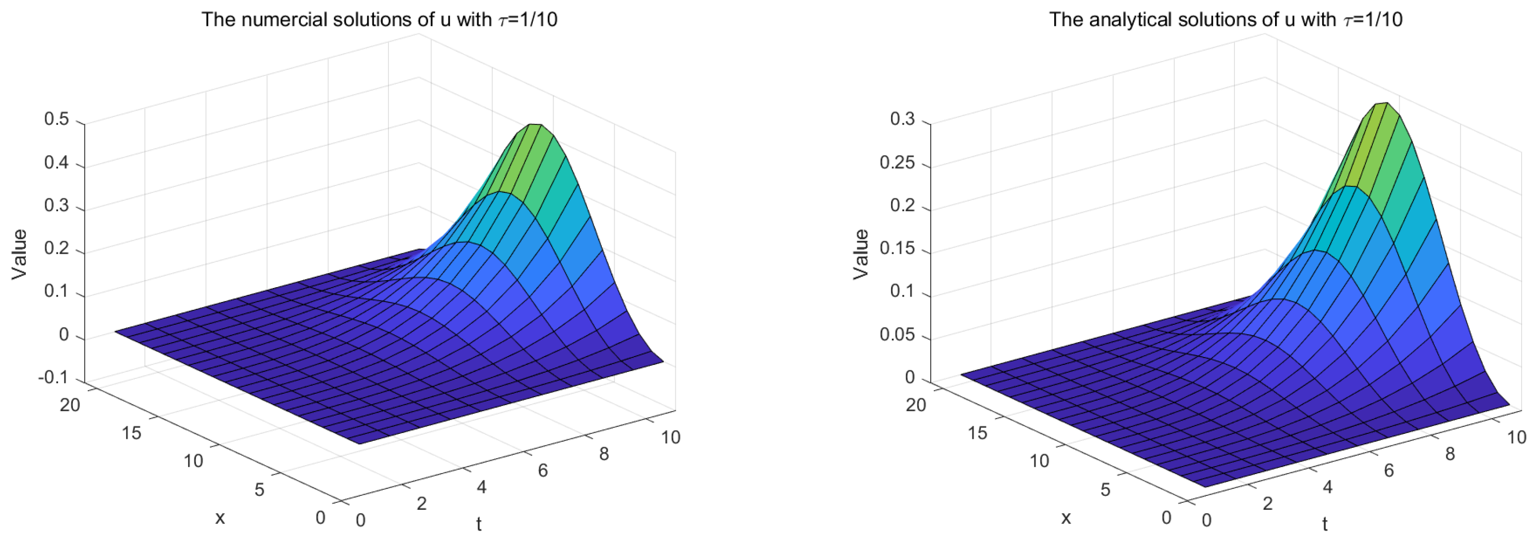
5.1. One-Dimensional Time-Fractional Fourth-Order System

Consider that the exact solution to the system is

$$\begin{array}{cc}\hfill & u(x,t)=t^{k}sin\left(\pi x\right)/k,x\in [0,1],t\in (0,1].\hfill \end{array}$$

(41)

In Figure 1, the two figures at the top depict the present solutions for the fractional-order system, with $M=21$, $\tau =10$, $\alpha =1.7$, and $k=3.5$. Even though errors are evidently present compared with the analytical solution with $\tau =1/10$, the complete congruence of the graph shapes vividly attests to the stability of the scheme format.

Taking $\alpha =1.5$ and $k=3.5$,

Table 1. Several numerical outcomes of the diverse space grid schemes ($\tau =1/320$).

$(\mathit{x},\mathit{t})$	5	7	9	11	13	Exact Solution
$(0.5,0.75)$	0.1046	0.1044	0.1044	0.1044	0.1044	0.1044
$(0.5,1)$	0.2863	0.2857	0.2857	0.2857	0.2857	0.2857

shows some numerical and exact solutions at the points $(0.5,0.75)$ and $(0.5,1)$ for diverse mesh sizes while maintaining a fixed temporal step. It is evident from this table that the current scheme converges expeditiously towards the exact solutions.

Table 2. Temporal convergence order of the proposed scheme $(M=21)$.

$\mathit{\tau }$	1/10	1/20	1/40	1/80	1/160	1/320	Value
$E_n$	7.1808 × 10−3	2.9680 × 10−3	1.2150 × 10−3	4.9515 × 10−4	2.0139 × 10−4	8.1845 × 10−5
Order		1.2746	1.2886	1.2950	1.2979	1.2991	1.3000

exhibits the temporal convergence order of the proposed scheme at $t=1$, which is in proximity to our theoretical values 1.3.

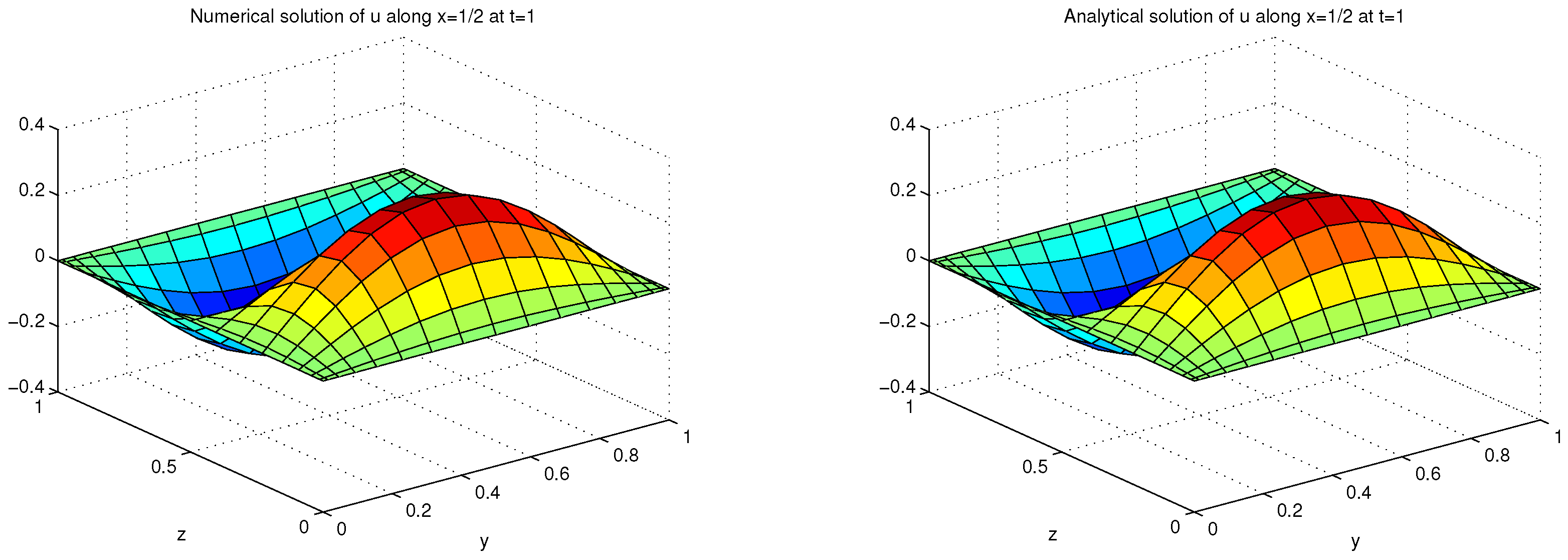
5.2. Two-Dimensional Time-Fractional Fourth-Order System

To implement numerical effectiveness, we consider the two-dimensional time-fractional fourth-order system that follows. The exact solution of the system is

$$\begin{array}{cc}\hfill & u(\mathbf{x},t)=t^{3+\alpha }sin\left(\pi x\right)sin\left(\pi y\right)+tsin\left(\pi x\right)sin\left(\pi y\right),\mathbf{x}\in {[0,1]}^2,t\in (0,1].\hfill \end{array}$$

(42)

Take $M=21$, and let $\alpha =1.7,1.5,1.3$, respectively.

Table 3. The convergence order in two-dimensional space at t = 1.

$\mathit{\tau }$	$\mathit{\alpha }=1.7$			$\mathit{\alpha }=1.5$			$\mathit{\alpha }=1.3$
	${\mathit{E}}_{\mathit{n}}$	Order		${\mathit{E}}_{\mathit{n}}$	Order		${\mathit{E}}_{\mathit{n}}$	Order
1/10	5.6317 × 10−3			2.6130 × 10−3			1.1484 × 10−3
1/20	2.1551 × 10−3	1.3858		9.3348 × 10−4	1.4850		3.6085 × 10−4	1.6701
1/40	8.4851 × 10−4	1.3448		3.3230 × 10−4	1.4901		1.1222 × 10−4	1.6851
1/80	3.3976 × 10−4	1.3204		1.1790 × 10−4	1.4949		3.4712 × 10−5	1.6928
1/160	1.3716 × 10−4	1.3086		4.1762 × 10−5	1.4973		1.0711 × 10−5	1.6964
1/320	5.5570 × 10−5	1.3035		1.4781 × 10−5	1.4985		3.3012 × 10−6	1.6980
1/640	2.2547 × 10−5	1.3015		5.2290 × 10−6	1.4991		1.0169 × 10−6	1.6988
1/1280	9.1538 × 10−6	1.3005		1.8495 × 10−6	1.4994		3.1317 × 10−7	1.6992
1/2560	3.7172 × 10−6	1.3002		6.5406 × 10−7	1.4996		9.6428 × 10−8	1.6994
Theoretical value		1.3000			1.5000			1.7000

presents specific numerical results related to the infinity norm errors and the convergence order for different temporal mesh sizes at t = 1. From these results, it can be observed that the temporal convergence order is approximately and close to $3-\alpha$.

In Figure 2, when $\tau =1/10$ and $\alpha =1.4$ at $t=1$, the surfaces of the numerical solution as well as the absolute error of u are depicted. It is readily observable that the numerical solutions are in extremely close proximity to the analytical solutions. By making a comparison between the two surfaces of u, it can be discerned that the surface of the absolute error coincides with that of the numerical results. A comparable conclusion concerning the relationship between the numerical solution and the absolute error of u is derived in Figure 2.

5.3. Three-Dimensional Time-Fractional Fourth-Order System

To implement the numerical effectiveness, the following fractional fourth-order system is considered. The analytical solution of this system is $u(\mathbf{x},t)={\displaystyle \frac{t^3}{3}}sin\left(\pi x\right)sin\left(\pi y\right)sin\left(2\pi z\right)$, $\mathbf{x}\in {[0,1]}^3$$,t\in (0,1]$. By setting $M=13$ and $\tau =1/20$, three comparisons of the surfaces between the exact solution and the numerical solution are exhibited, along with the condition $x=1/2$ at $t=1$ when taking $\alpha =1.6$ into account in Figure 3.

Let $\alpha$ assume the values 1.3, 1.5, and 1.7, respectively.

Table 4. The convergence order in three-dimensional space at t = 1.

$\mathit{\tau }$	$\mathit{\alpha }=1.3$			$\mathit{\alpha }=1.5$			$\mathit{\alpha }=1.7$
	${\mathit{E}}_{\mathit{n}}$	Order		${\mathit{E}}_{\mathit{n}}$	Order		${\mathit{E}}_{\mathit{n}}$	Order
1/10	2.1249 × 10−4			4.9392 × 10−3			9.7883 × 10−3
1/20	6.6285 × 10−4	1.6806		1.7756 × 10−4	1.4760		3.9602 × 10−3	1.3055
1/40	2.0573 × 10−5	1.6979		6.3224 × 10−5	1.4897		1.6177 × 10−4	1.2916
1/80	6.3850 × 10−5	1.6880		2.2444 × 10−5	1.4942		6.6040 × 10−5	1.2925
1/160	1.9992 × 10−6	1.6752		7.9736 × 10−6	1.4930		2.6878 × 10−5	1.2946
1/320	6.4637 × 10−7	1.6291		2.8493 × 10−6	1.4846		1.0932 × 10−5	1.2945
Theoretical value		1.7000			1.5000			1.3000

presents specific numerical results related to the maximum errors and the corresponding temporal convergence order for different temporal mesh sizes at t = 1. From these results, it can be observed that the temporal convergence order is approximately and closely equal to $3-\alpha$.

6. Conclusions

In this paper, we present a compact difference-Galerkin spectral scheme for coupledly solving a multi-dimensional variable coefficient time-fractional fourth-order partial differential system. The main conclusions of this article, including the stability, convergence, and solvability of the method, were derived. Finally, some computational experiments are illustrated to demonstrate the superiority of the compact difference-Galerkin method. Lastly, we plan to carry out a multitude of subsequent works, including ones on special boundary conditions, discontinuous solutions, and so on.

References

1. Samko, S.G.; Kilbas, A.A.; Marichev, O.I. Fractional Integrals and Derivatives: Theory Applications; Gordon and Breach Science: New York, NY, USA, 1993. [Google Scholar]
2. Podlubny, I. Fractional Differential Equations; Academic Press: New York, NY, USA, 1999. [Google Scholar]
3. Kilbas, A.A.; Srivastava, H.M.; Trujillo, J.J. Theory and Applications of Fractional Differential Equations; North-Holland: New York, NY, USA, 2006. [Google Scholar]
4. Baleanu, D.; Diethelm, K.; Scalas, E.; Trujillo, J.J. Fractional Calculus Models and Numerical Methods; Series on Complexity, Nonlinearity and Chaos; World Scientific: Singapore, 2012. [Google Scholar]
5. Sun, H.; Zhang, Y.; Baleanu, D.; Chen, W.; Chen, Y. A new collection of real world applications of fractional calculus in science and engineering. Commun. Nonlinear Sci. Numer. Simul. 2018, 64, 213–231. [Google Scholar] [CrossRef]
6. Li, X.; Xu, C. A space-time spectral method for the time fractional diffusion equation. SIAM J. Numer. Anal. 2009, 47, 2108–2131. [Google Scholar] [CrossRef]
7. Zhao, J.; Xiao, J.; Xu, Y. Stability and convergence of an effective finite element method for multiterm fractional partial differential equations. Abstr. Appl. Anal. 2013, 2013, 857205. [Google Scholar] [CrossRef]
8. Zhuang, P.; Gu, Y.T.; Liu, F.; Turner, I.; Yarlagadda, P.K.D.V. Time-dependent fractional advection-diffusion equations by an implicit MLS meshless method. Int. J. Numer. Methods Eng. 2011, 88, 1346–1362. [Google Scholar] [CrossRef]
9. Gu, X.M.; Sun, H.W.; Zhao, Y.L.; Zheng, X. An implicit difference scheme for time-fractional diffusion equations with a time-invariant type variable order. Appl. Math. Lett. 2021, 120, 107270. [Google Scholar] [CrossRef]
10. Mandelbrot, B.B. The Fractal Geometry of Nature; WH Freeman: New York, NY, USA, 1982. [Google Scholar]
11. Caputo, M. Elasticitàe Dissipazione; Zanichelli: Bologna, Italy, 1969. [Google Scholar]
12. Caputo, M.; Mainardi, F. Linear models of dissipation in an elastic solids. Riv. Nuevo Clmento (Ser. II) 1971, 1, 161–198. [Google Scholar]
13. Bagley, R. Applications of Generalized Derivatives of Viscoelasticity. Ph.D. Thesis, Air Force Institute of Technology, Wright-Patterson AFB, OH, USA, 1979. [Google Scholar]
14. Golbabai, A.; Sayevand, K. Fractional calculus—A new approach to the analysis of generalized fourth-order diffusion-wave equations. Comput. Math. Appl. 2011, 67, 2227–2231. [Google Scholar] [CrossRef]
15. Jafari, H.; Dehghan, M.; Sayevand, K. Solving a fourth-order fractional diffusion wave equation in a bounded domain by decomposition method. Numer. Methods Partial. Differ. Equ. 2008, 24, 1115–1126. [Google Scholar] [CrossRef]
16. Agrawal, O.P. A general solution for a fourth-order fractional diffusion-wave equation defined in a bounded domain. Comput. Struct. 2001, 79, 1497–1501. [Google Scholar] [CrossRef]
17. Oldham, K.B.; Spanier, J. The Fractional Calculus; Academic Press: Cambridge, MA, USA, 1974. [Google Scholar]
18. Vong, S.; Wang, Z. Compact finite difference scheme for the fourth-order fractional subdiffusion system. Adv. Appl. Math. Mech. 2014, 6, 419–435. [Google Scholar] [CrossRef]
19. Hu, X.L.; Zhang, L.M. On finite difference methods for fourth-order fractional diffusion-wave and subdiffusion systems. Appl. Math. Comput. 2012, 218, 5019–5034. [Google Scholar] [CrossRef]
20. Liu, Y.; Du, Y.W.; Li, H.; Li, J.C.; He, S. A two-grid mixed finite element method for a nonlinear fourth-order reaction diffusion problem with time-fractional derivative. Comput. Math. Appl. 2015, 70, 2474–2492. [Google Scholar] [CrossRef]
21. Liu, Y.; Du, Y.W.; Li, H.; He, S.; Gao, W. Finite difference/finite element method for a nonlinear time-fractional fourth-order reaction-diffusion problem. Comput. Math. Appl. 2015, 70, 573–593. [Google Scholar] [CrossRef]
22. Dehghan, M.; Manafian, J.; Saadatmandi, A. The solution of the linear fractional partial differential equations using the homotopy analysis method. Z. Naturforschung-A 2010, 65, 935–949. [Google Scholar] [CrossRef]
23. Dehghan, M.; Manafian, J.; Saadatmandi, A. Solving nonlinear fractional partial differential equations using the homotopy analysis method. Numer. Methods Partial. Differ. Equ. 2010, 26, 448–479. [Google Scholar] [CrossRef]
24. Zhang, H.; Liu, F.; Phanikumar, M.S.; Meerschaert, M.M. A novel numerical method for the time variable fractional order mobile-immobile advection–dispersion model. Comput. Math. Appl. 2013, 66, 693–701. [Google Scholar] [CrossRef]
25. Parvizi, M.; Eslahchi, M.R.; Dehghan, M. Numerical solution of fractional advection-diffusion equation with a nonlinear source term. Numer. Algorithms 2015, 68, 601–629. [Google Scholar] [CrossRef]
26. Tang, T.; Jie, S. Spectral and High-Order Methods with Applications; Science Press: Alexandria, NSW, Australia, 2006. [Google Scholar]
27. Yi, S.C.; Yao, L.Q. A steady barycentric lagrange interpolation method for the 2d higher order time-fractional telegraph equation with nonlocal boundary condition with error analysis. Numer. Methods Partial. Differ. Equ. 2019, 35, 1694–1716. [Google Scholar] [CrossRef]
28. Sun, Z.Z.; Wu, X.N. A fully discrete difference scheme for a diffusion-wave system. Appl. Numer. Math. 2006, 56, 193–209. [Google Scholar] [CrossRef]
Figure 1. The curved surfaces of the numerical solution u (left) and the analytical solution (right).
Fractalfract 09 00155 g001
Figure 2. The curved surfaces of the numerical solution u (left) and absolute error (right).
Fractalfract 09 00155 g002
Figure 3. The curved surfaces for the numerical solutions (left) and exact solutions (right).
Fractalfract 09 00155 g003