Continuous Adaptive Stabilization of the Unstable Period-1 Orbit of the Fractional Difference Logistic Map

Abstract

A continuous adaptive stabilization technique for the unstable period-1 orbit of the fractional difference logistic map is presented in this paper. An impulse-based control technique without short oscillatory transients right after the control impulse is designed for the fractional map with a long memory horizon. However, it appears that the coordinate of the unstable period-1 orbit may drift due to the continuous application of the impulse-based control scheme. An adaptive scheme capable of tracking the drifting coordinate of the unstable period-1 orbit is designed and validated by a number of computational experiments. The proposed control scheme is minimally invasive compared to the continuous feedback control as it preserves the model of the system while requiring only a series of sparse, small, instantaneous control impulses to achieve continuous adaptive stabilization of the unstable period-1 orbit of the fractional difference logistic map.

1. Introduction

Discrete fractional maps have recently received attention in various fields of science and engineering [1]. Fractional maps find applications in diverse fields, starting from informatics (information security [2], encryption [3], and image processing [4]) and finishing with engineering [5] and medicine [6].

The stabilization and control of discrete fractional maps remain challenging and significant. Unlike their integer-order counterparts, discrete fractional maps exhibit unique properties such as non-locality and memory effects. The state of such maps is determined not only by local values but also by a substantial portion—or, in some cases, the entirety—of past states [7].

Chaos and its control in discrete fractional maps are explored in [8,9]. The stability of fractional logistic maps and their lattices is investigated in [10,11]. The dynamics and control of fractional Ikeda map are studied in [12], while the stability and control of a fractional system with delays are investigated in [13]. A feedback control scheme for the fractional difference logistic map based on permutation entropy and fuzzy logic is constructed in [14]. A backstepping method for the control of fractional single-input single-output systems is constructed in [15]. Containment control is successfully applied to discrete-time fractional-order multi-agent systems with a time delay in [16]. Impulse control techniques applicable to chaotic fractional systems are presented in [17,18].

One of the most important topics in chaos control of nonlinear systems is the stabilization of unstable periodic orbits [19]. Numerous different techniques and approaches have been developed for the stabilization of unstable periodic orbits in the last few decades [20,21].

However, fractional-order models (continuous and discrete) do not exhibit periodic orbits [22]. Nevertheless, some trajectories of discrete fractional maps may exhibit asymptotic periodicity after a number of iterations—such trajectories are called asymptotically periodic, and the manifold that such an orbit approaches is called an asymptotic period-k sink [23]. The only truly periodic orbit of the fractional difference logistic map is the period-1 orbit [24]. A more detailed treatment of this classification is given in Section 2.2.

Finite-time stabilization of the unstable period-1 orbit of the fractional difference logistic map was introduced in [25]. The approach proposed in [25] relies on an impulsive perturbation applied at a specific time step. This stabilization method is less invasive than feedback control, as it preserves the original model of the fractional difference logistic map and requires only a small instantaneous perturbation to achieve finite-time stabilization. The primary objective of this paper is to eliminate transient oscillations following the control impulse and to propose a continuous adaptive stabilization scheme of the unstable period-1 orbit of the fractional difference logistic map.

The main motivation of this objective is to address a critical practical issue: in many real-world applications, such as electrical circuits, even short transient oscillations can lead to significant damage. We aim to develop a control strategy that not only achieves finite-time stabilization of the unstable period-1 orbit but also eliminates these undesirable oscillatory transients. Furthermore, the inherent long memory of fractional difference logistic maps causes the trajectory to drift, necessitating an adaptive scheme that continuously tracks and compensates for this drift to maintain system performance within strict tolerance bounds.

This paper is structured as follows. Preliminaries and our motivation are given in Section 2. The control scheme without oscillatory transients in introduced in Section 3. The drift of the period-1 orbit is discussed in Section 3.3; the adaptive control scheme capable of tracking the drifting coordinate of the unstable period-1 orbit is presented in Section 3.4. Finally, concluding remarks are given in Section 4.

2. Preliminaries and Motivation

2.1. The Fractional Difference Logistic Map

The fractional difference logistic map is defined as follows [23,26]:

$$x_{k+1}=x_0+\sum _{i=1}^{k+1}{G}_{i-1}^{\alpha }\left(a{x}_{k-i+1}\left(1-x_{k-i+1}\right)-x_{k-i+1}\right),k=0,1,\dots ,$$

(1)

where $G_0^{\alpha }=1,G_i^{\alpha }=\left(1-{\displaystyle \frac{1-\alpha }{i}}\right)G_{i-1}^{\alpha },i=1,2,\dots ,k+1$. The parameter $\alpha \in (0,1]$ represents the fractional order of Equation (1). Please note that setting $\alpha =1$ reduces (1) to the classical logistic map.

Unlike the classical logistic map, the present state $x_k$ in the fractional map (Equation (1)) depends not only on the previous state $x_{k-1}$, but on all the past states $x_{k-1},x_{k-2},\dots ;x_0$. In other words, the memory horizon of the fractional difference logistic map reaches the initial condition. Furthermore, the fractional difference logistic map is a non-invertible discrete map that utilizes the Caputo fractional difference definition [23,27,28].

2.2. Periodicity in the Fractional Difference Logistic Map

By definition, a period-k orbit consists of a sequence $x_0,x_1,\dots$, generated by (1) such that the sequence has k infinitely repeating elements: $x_0,x_1,\dots ,x_{k-1},x_0,x_1,\dots ,x_{k-1},x_0,\dots$. It has been proven that the fractional difference logistic map possesses only a period-1 orbit [23,24].

However, the fractional difference logistic map does have asymptotic period-k sinks [29]. This means that the map (1) can generate a sequence which, after a number of transient iterations, exhibits asymptotic period-k behavior. The k points that the map’s trajectory alternates between in this behavior form the asymptotic period-k sink. It is important to note that this process is inherently asymptotic and always includes transient processes, since there are no period-k, $k>1$ orbits.

For simplicity and readability, we will refer to trajectories of the fractional difference logistic map that approach a period-k sink as period-kregimes to distinguish them from a period-k orbit.

2.3. The Finite-Time Stabilization of Unstable Period-1 Orbits of the Fractional Difference Logistic Map

It has been shown in [25] that a small control impulse can achieve finite-time stabilization of unstable orbits in the fractional difference logistic map. Such a finite-time stabilization scheme is coined as the H-rank based impulse control scheme [25] and is illustrated in Figure 1.

Let us assume that the tolerance corridor around the unstable period-1 orbit of the fractional difference logistic map is $\delta =0.1$ (presented as horizontal dotted lines in Figure 1). In other words, as long as the trajectory is contained in this corridor, no control is applied to the system. However, once the trajectory violates the boundaries of the tolerance corridor at $k=86$ (this iteration is marked by the vertical dashed green line in Figure 1), the H-rank impulse control scheme is immediately executed at this step.

As mentioned, in this case (see Figure 1), the control impulse is applied at $k=86$. This specific value is not arbitrary; it represents the first time step at which the system’s trajectory breaches the predefined tolerance corridor $\delta =0.1$ around the unstable period-1 orbit. At $k=86$, the deviation becomes significant enough to trigger the H-rank impulse control scheme. It is important to note that while $k=86$ serves as a reference point in our current example, its value varies depending on the width of the tolerance corridor, the chosen system parameters, and initial conditions.

As previously established, the memory horizon of the fractional difference logistic map extends back to the initial condition. Consequently, the system’s evolution after the control impulse depends not only on $x_{86}$ (immediately following the application of the control impulse) but also on the entire preceding trajectory. Considering this, a pattern of H-ranks is plotted for all possible evolutions of the system after $x_{86}$ (Figure 1).

The H-rank control scheme proposed in [25] relies on selecting the deepest trench in the H-rank pattern. This is illustrated by the black circle marker in the H-rank pattern in Figure 1. In other words, the coordinate of $x_{86}$ after the control impulse is set to $0.4821$, which coincides with the position of the marker in the H-rank pattern (Figure 1b).

The evolution of the system without control is depicted in light gray in Figure 1a (the system asymptotically converges to the stable period-2 regime). In contrast, the evolution of the system after control is shown in blue in Figure 1a. Initially, the system exhibits finite-time convergence to the unstable period-1 orbit. However, after a number of iterations, the system diverges from the unstable period-1 orbit and asymptotically converges to the stable period-2 regime (Figure 1a).

Note that the naive control scheme (when the control impulse brings the system into the coordinate corresponding to the unstable period-1 orbit) is insufficient. The fractional difference logistic map quickly converges to the stable period-2 regime in a few time-forward iterations after such a control impulse [25].

2.4. The Motivation for the Further Development of the Control Scheme

The finite-time stabilization technique of unstable orbits or regimes of the fractional difference logistic map, as introduced in [25], can be extended to a continuous stabilization scheme [25]. In this case, a secondary control impulse would be applied whenever the blue trajectory violates the tolerance corridor in Figure 1a). However, the fractional difference logistic map exhibits a brief but violently oscillatory transient behavior immediately after the control impulse [25].

The objective and motivation for further development of the control scheme for the stabilization of unstable orbits or regimes of the fractional difference logistic map is based on the desire to eliminate this brief and violent oscillatory transient behavior immediately after the control impulse. The rationale for such a control scheme could be explained by possible engineering applications. For example, the period-1 orbit could represent the zero current in an electrical circuit. The tolerance corridor could represent the maximum positive and the maximum negative current allowed in the circuit. Clearly, short violent transient oscillations would damage the circuit. The ability to continuously keep the current in the tolerance corridor (even though the period-1 orbit is unstable) would be of primary importance for such a control scheme.

3. The Control Scheme Without Oscillatory Transients

3.1. The Feasibility of the Proposed Approach

The original control scheme depicted in Figure 1 is designed to find the deepest trench in the H-rank pattern, thus achieving the longest finite-time stabilization of the unstable period-1 orbit [25]. However, the H-rank pattern in Figure 1b reveals several trenches, which are further explored in Figure 2. Note that all computations in Figure 2 are performed using the same set of parameters as in Figure 1, except for the coordinate $x_{86}$, which is set to the middle of different trenches in the the H-rank pattern (rather than exclusively choosing the one leading to the longest finite state stabilization of the unstable orbit). Furthermore, note that the H-rank pattern is now placed horizontally (Figure 2).

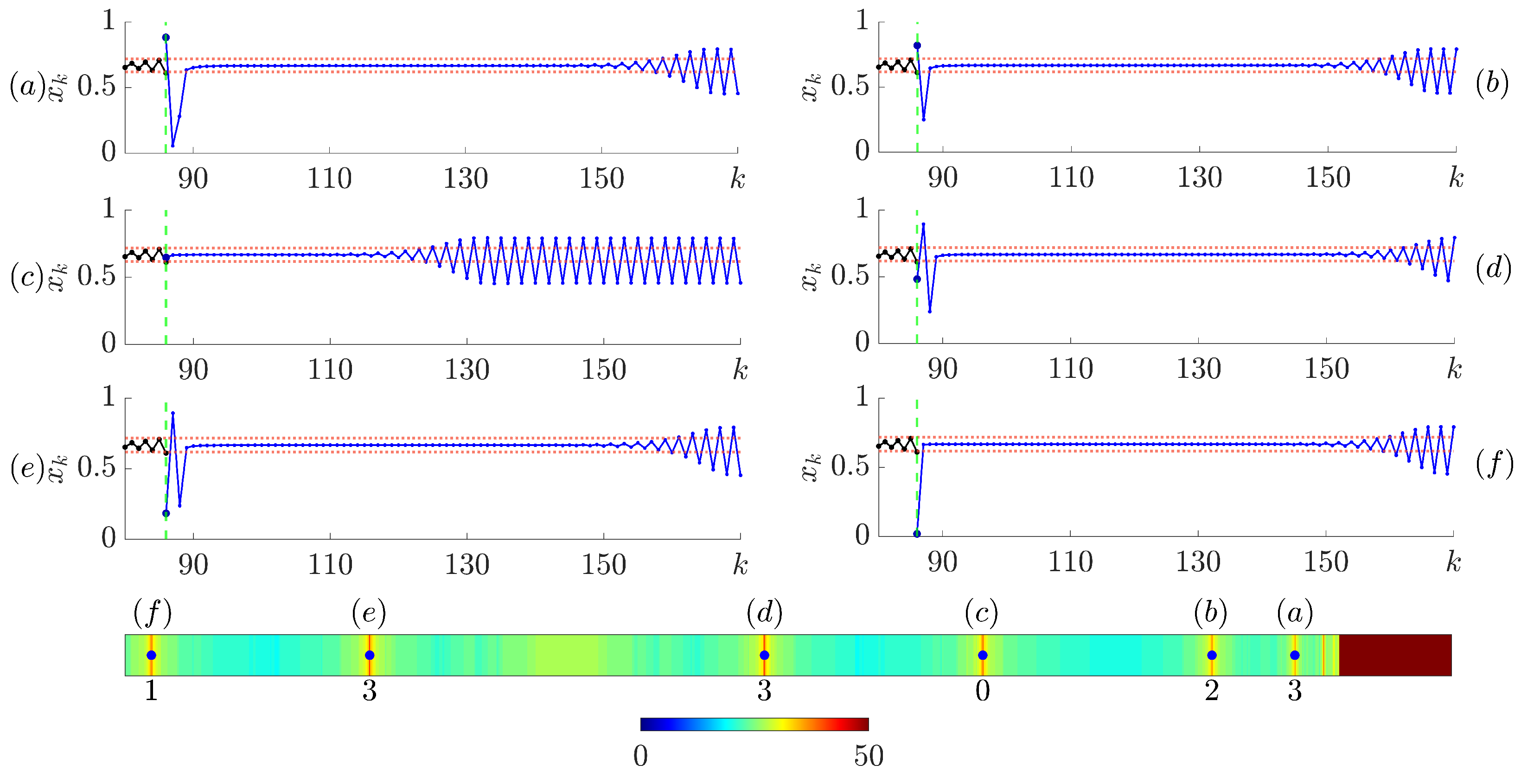
The trenches in the H-rank pattern are enumerated from (a) to (f) (Figure 2). The transient processes following the control impulse are visualized in six corresponding sub-panels (a to f). Note that the finite-time stabilization of the unstable period-1 orbit is achieved in all six cases. However, the key differences lie in the duration and shape of the brief oscillatory transient behavior immediately following the control impulse.

The numbers below each of the trenches in the pattern of H-ranks in Figure 2 denote the number of time steps until the transient trajectory exceeds the tolerance corridor immediately following the control impulse. Notably, the number of steps during which the trajectory remains inside the tolerance corridor after the control impulse and after the short oscillatory transient is different. The trajectory remains inside the tolerance corridor for 70 steps in panel (a), 71 steps in panel (b), 38 steps in panel (c), 74 steps in panel (d), 71 steps in panel (e) and 72 steps in panel (f). Note that panel (d) is the exact copy of Figure 1.

Interestingly, the transient process depicted in Figure 2c does not exhibit the violent oscillatory transient typically observed immediately following the control impulse, despite the finite-time stabilization of the period-1 orbit being significantly shorter than the optimal situation in Figure 2d. Moreover, it is important to emphasize that the control impulse does not place the trajectory directly onto the unstable period-1 orbit. In other words, the naive control method continues to be ineffective, as previously noted in [25]).

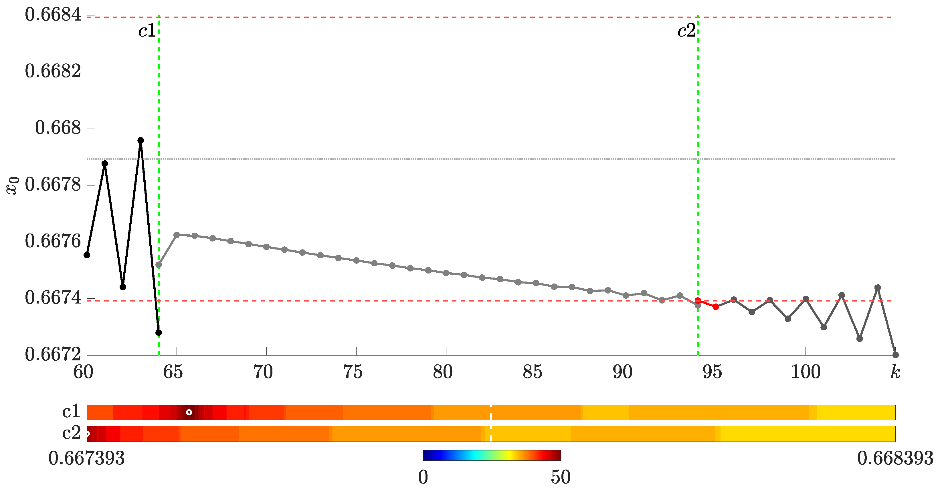
This fact is illustrated in Figure 3. This figure replicates the finite-time stabilization of the unstable period-1 orbit depicted in Figure 2c. The trajectory of the system until step $k=86$ is plotted in black. The trajectory after the control impulse is plotted in blue; the coordinate after the control impulse is also marked by a blue dot in the H-rank pattern in Figure 3. In the naive control scheme (as defined in [25]) it is implied that the coordinate after the control impulse is set to the unstable period-1 orbit. The trajectory resulting from the naive control scheme is plotted in red; the coordinate after the control impulse is also marked by a red dot on the H-rank pattern in Figure 3.

3.2. Continuous Stabilization of the Unstable Period-1 Orbit

Having established that it is possible to avoid short transient oscillations right after the control impulse, it is important to understand whether the repetitive application of such control impulses can continuously stabilize the system inside the tolerance corridor around the unstable period-1 orbit.

Let us continue with the stabilization scheme depicted in Figure 2c (the width of the tolerance corridor is set to $\delta =0.1$). The first control impulse is executed at $k=86$ when the trajectory violates the boundaries of the tolerance corridor. This instance is marked by $c1$ in Figure 4 (both in the time plot and the zoomed-in part of the H-rank pattern).

However, instead of waiting for the transient trajectory to converge to the period-2 regime after the first control impulse, the control scheme is reapplied immediately when the trajectory breaches the boundaries of the tolerance corridor for the second time. In particular, the H-rank pattern after the second control impulse differs slightly from the pattern after the first control impulse. This discrepancy arises because the subsequent evolution of the system is predetermined by all previous states (including the first control impulse) because of the long memory horizon of the fractional map.

Only the first two control impulses $c1$ and $c2$ are visualized on the H-rank pattern. However, the red dots denoting the coordinates after each control impulse are depicted throughout the time plot in Figure 4 (every second transient trajectory is shown in gray for clarity).

Similar calculations are performed using an identical computational setup, except with a narrower tolerance corridor ($\delta =0.01$; Figure 5). The continuous stabilization strategy is effective, although it is noticeable that the period-1 orbit is not completely stationary, especially at the beginning of the continuous stabilization process (Figure 5).

However, further reducing the width of the tolerance corridor to $\delta =0.001$ interrupts the continuous stabilization process (Figure 6). The first stabilization control impulse $c1$ remains effective, providing finite-time stabilization of the transient process. However, the stabilized trajectory gradually drifts downward (Figure 6). While this drift is generally small, it eventually exceeds the border of the tolerance corridor, which is also narrow). In particular, the trench in the H-rank pattern for the control impulse $c2$ is no longer located inside the designated tolerance corridor (Figure 6), and the continuous stabilization of the unstable period-1 orbit becomes impossible.

3.3. The Drift of the Period-1 Orbit

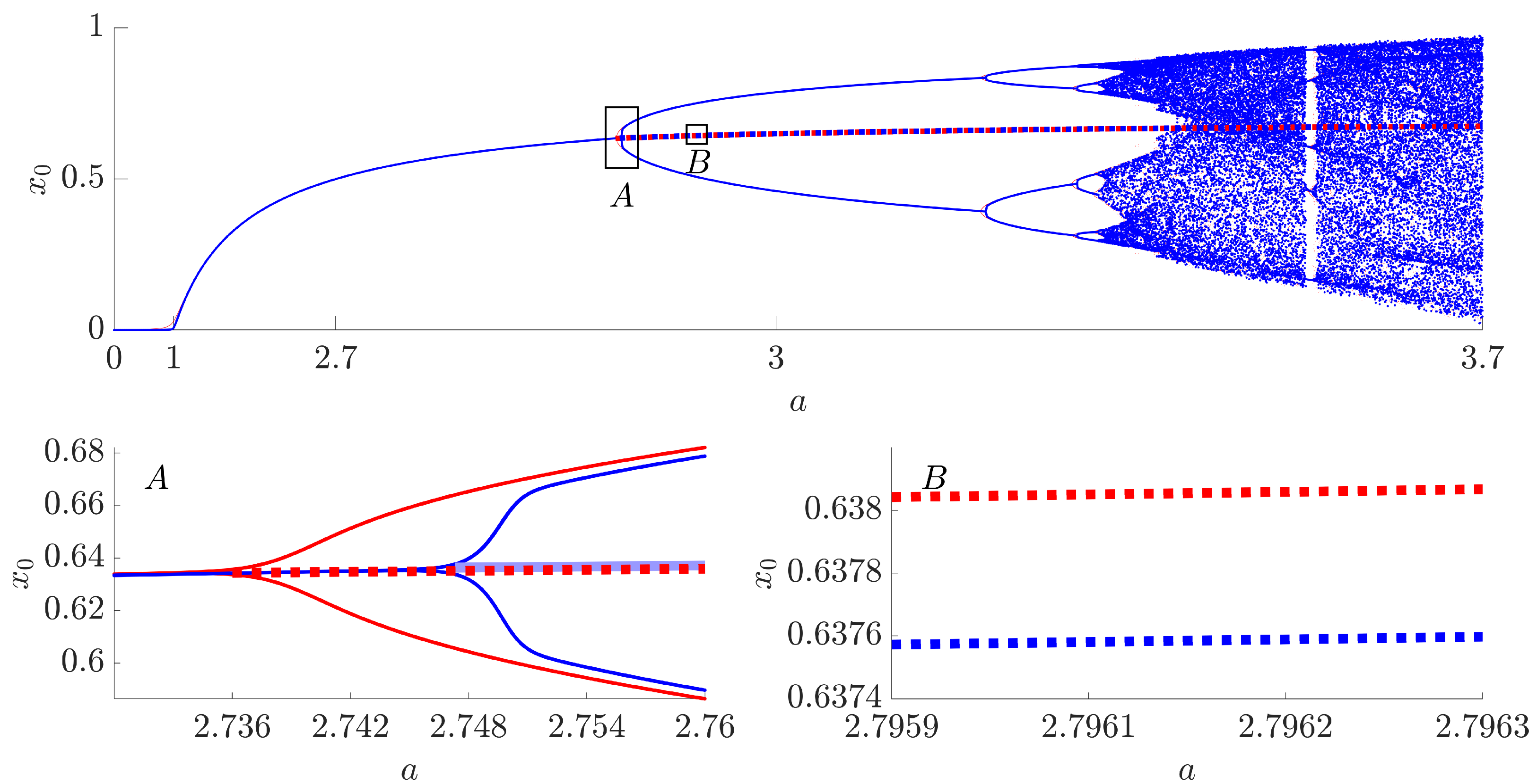
It has already been reported in [30] that the bifurcation diagram of the fractional difference logistic map varies with different initial conditions. While these differences are small, they are still interpretable (panel (A), Figure 7). The red bifurcation diagram is constructed by setting the initial condition $x_0$ to $0.9999$; the blue bifurcation diagram is constructed by setting $x_0$ to $0.062$. The resulting bifurcation diagram in Figure 7 predominantly appears blue, as the blue dots largely overlap with the red ones. However, panel (A) reveals small but substantial differences in and around the first period doubling bifurcation.

Note that in constructing the bifurcation diagram given in Figure 7, a total of 10,000 iterations were skipped in order to make the map move past transient processes. This was done for both $x_0=0.9999$ (red line) and $x_0=0.062$ (blue line). Due to this, even though the fractional difference logistic map does not posses periodic orbits (as discussed in Section 2.2), skipping the transient processes does allow to depict periodic regimes on the bifurcation diagram.

This effect can be explained by the long memory horizon of the fractional difference logistic map. Interestingly, there is a noticeable relationship between the initial condition $x_0$ and the exact location of the first period-doubling bifurcation (Figure 8).

However, this effect has another implication, which is illustrated in panel (B) of Figure 7. Starting earlier, the red period-doubling bifurcation leads to the unstable period-1 orbit that is positioned below the blue period-1 orbit (panel (B)). While the difference may initially appear negligible, it becomes significant when the width of the tolerance corridor $\delta$ becomes sufficiently small.

Moreover, the results depicted in Figure 7 and Figure 8 are produced by only changing the initial condition $x_0$. The situation becomes considerably more complex when repetitive control impulses are employed to stabilize the unstable trajectory within the tolerance corridor. The long memory horizon of the fractional difference logistic map implies that the system retains all perturbations from the initial condition to the current moment. As a result, stabilizing unstable orbits or regimes within a narrow tolerance corridor requires a technique that could automatically track the drift of the unstable period-1 orbit, even if that drift is substantially small.

3.4. Continuous Stabilization of the Unstable Period-1 Orbit in Narrow Tolerance Corridors

As mentioned in the previous section, a small drift of the unstable period-1 orbit can compromise the proposed stabilization technique when the width of the tolerance corridor is sufficiently small. Since all previous time steps (including the control impulses) have an impact on the future evolution of the system, it is necessary to create a technique capable of automatically self-adjusting to dynamically changing conditions.

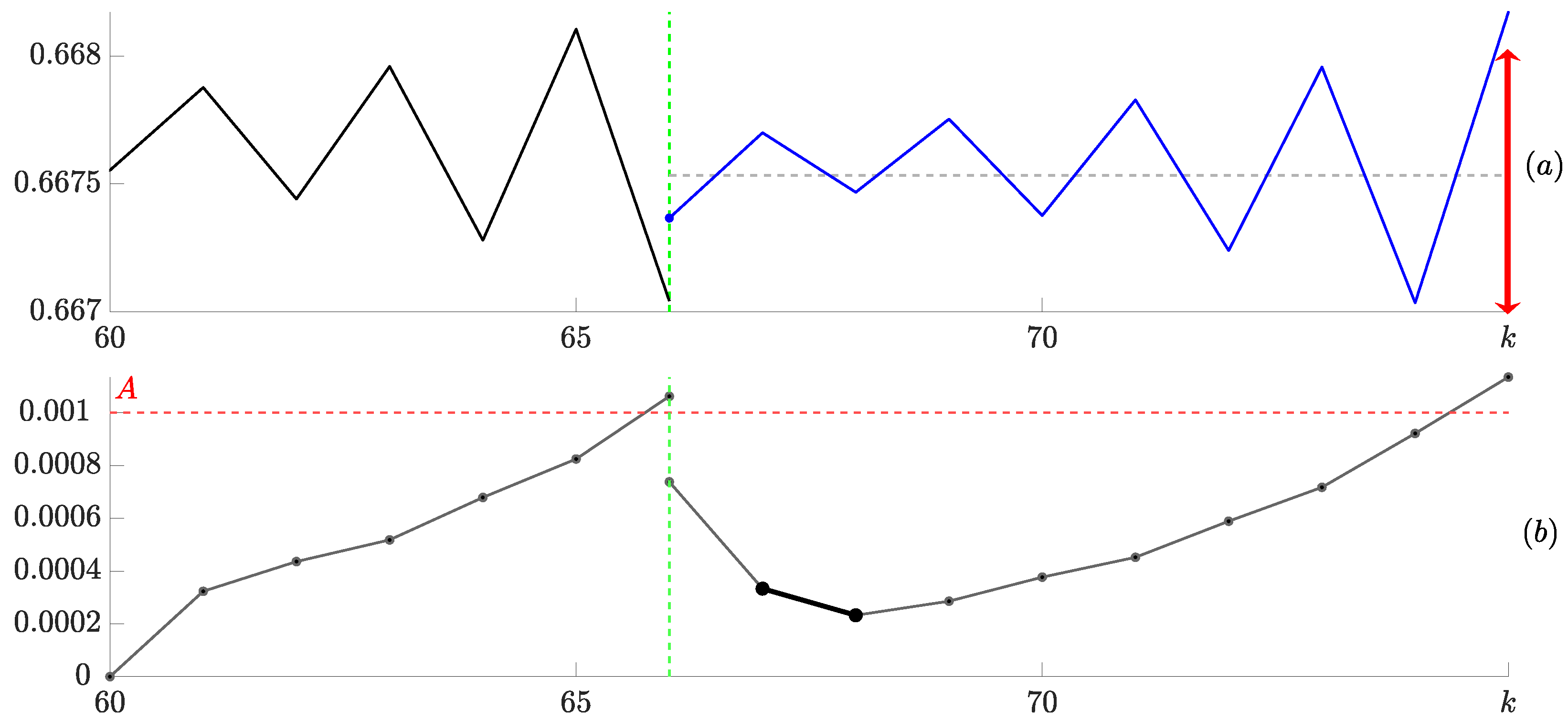
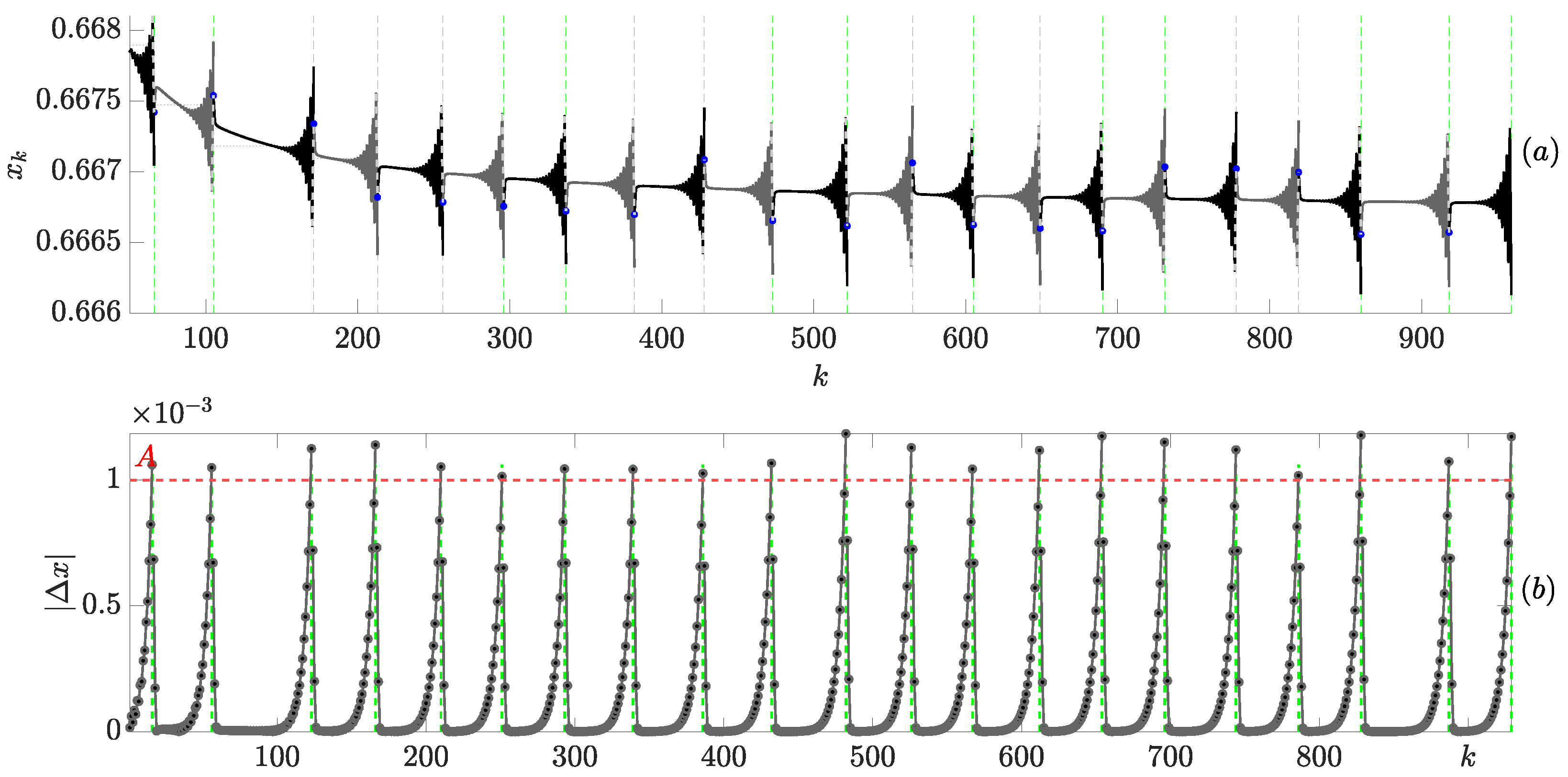
The main idea of such a technique is illustrated in Figure 9. Instead of setting a static tolerance corridor, we introduce the threshold A for the absolute difference of the two adjacent time steps (panel (b), Figure 9). The absolute differences exceed the threshold A at $k=66$, and the control impulse places the system coordinate in the middle of the trench residing in the H-rank pattern (which is omitted in Figure 9). As the blue trajectory evolves, two consecutive steps, where the absolute differences values are the smallest, are identified (marked by the bold line in panel (b), Figure 9). Then, the drifted location of the unstable period-1 orbit is set to $x_{\ast }=\min \left({\displaystyle \frac{x_{k-1}+x_k}{2}}\right)$ (denoted as the blue dashed horizontal line in panel (a), Figure 9). Then, the observation window for the pattern of H-ranks (which is used at the moment when the absolute differences of adjacent points of the blue trajectory exceeds the threshold A) is set to $[x_{\ast }-{\displaystyle \frac{A}{2}};x_{\ast }+{\displaystyle \frac{A}{2}}]$ (denoted at the red vertical arrow in panel (a) Figure 9).

This approach guarantees that the finite stabilization technique is capable of tracking the drifting coordinate of the unstable period-1 orbit. The idea of selecting $x_{\ast }=\min \left({\displaystyle \frac{x_{k-1}+x_k}{2}}\right)$ is straightforward: one must wait for small transient oscillations to subside immediately after the control impulse, but act before the onset of oscillations that signal the start of asymptotic convergence to the stable period-2 regime.

The continuous adaptive stabilization scheme is illustrated in Figure 10 and Figure 11. In this approach, 20 control impulses are applied at specific moments to maintain the trajectory of the fractional difference logistic map within a narrow tolerance corridor around the drifting unstable period-1 orbit (Figure 10). As previously explained, the adaptive scheme applies impulses not when the trajectory exceeds the boundaries of the tolerance corridor, but when the absolute difference $\left|\Delta x\right|=\left|x_k-x_{k-1}\right|$ of the adjacent values surpasses the threshold A (the dashed red line in Figure 11b). This control method can indefinitely maintain the trajectory around the drifting unstable period-1 orbit.

4. Concluding Remarks

Finite-time stabilization of the unstable period-1 orbit of the fractional difference logistic map by using a single control impulse is a problem that can be characterized by its misleading apparent simplicity. Because the memory horizon of fractional difference maps extends to the initial condition, controlling the evolution of this fractional system by applying a single control impulse is completely unprecedented.

However, it appears that such finite-time stabilization of the unstable period-1 orbit of the fractional difference logistic map is possible (it has already been reported in [25]). This paper makes a twofold contribution to the state of the art in the dynamics of discrete fractional systems.

Firstly, this paper introduces a finite-time stabilization technique for the unstable period-1 orbit that circumvents violent transient oscillations immediately following the control impulse, which inevitably occur in the control algorithm presented in [25]).

Secondly, this paper presents an adaptive technique capable of tracking the drifting coordinate of the unstable period-1 orbit as the width of the tolerance corridor becomes exceedingly small. This technique facilitates continuous and indefinite stabilization of the unstable period-1 orbit of discrete fractional maps.

In contrast to earlier methods that directly place the system on the unstable period-1 orbit, resulting in pronounced oscillatory transients, our approach selects control impulses based on an analysis of the H-rank pattern to significantly mitigate these transients. Furthermore, by incorporating an adaptive strategy that tracks the drift of the period-1 orbit, our method continuously compensates for deviations even in very narrow tolerance corridors. This improvement not only enhances the smoothness of the stabilization process, but also makes the technique more robust and practical for applications where transient oscillations can be detrimental.

As already mentioned in the Introduction, many discrete and continuous systems can be stabilized by using continuous feedback loops. The design of a stabilization technique for a fractional difference system without a feedback loop is the main objective of this paper. A natural choice to test this stabilization technique is to use the fractional counterpart of the paradigmatic logistic map. The ability to cope with the fractional difference logistic map opens doors to the stabilization of the whole class of other fractional difference maps (the fractional difference standard map would probably be the first candidate). Clearly, the use of the proposed stabilization method for other fractional difference maps is the next objective of future research.

It should be noted that there exist different versions of fractional logistic maps (a typical version of the fractional logistic map is investigated in [31]). However, the fractional difference logistic map is reduced to the classical logistic map when the fractional order $\alpha$ tends to 1 (which is not the case with [31]). Therefore, this is a natural choice to explore a fractional model which is a natural extension of its non-fractional counterpart.

It is widely accepted that stable and unstable period-k orbits of the fractional difference logistic map do not exist when $k\ge 2$. The exploration of techniques for finite-time stabilization of higher-order unstable periodic regimes (rather than orbits) of discrete fractional maps remains a challenging objective for future research.

References

1. Ouannas, A.; Batiha, I.M.; Pham, V.T. Fractional Discrete Chaos: Theories, Methods and Applications; World Scientific: Singapore, 2023; Volume 3. [Google Scholar]
2. Liu, Z.; Xia, T.; Wang, T. Dynamic analysis of fractional-order six-order discrete chaotic mapping and its application in information security. Optik 2023, 272, 170356. [Google Scholar] [CrossRef]
3. Liu, Z.Y.; Xia, T.C.; Hu, Y. Dynamic analysis of new two-dimensional fractional-order discrete chaotic map and its application in cryptosystem. Math. Methods Appl. Sci. 2023, 46, 12319–12339. [Google Scholar] [CrossRef]
4. Talhaoui, M.Z.; Wang, X. A new fractional one dimensional chaotic map and its application in high-speed image encryption. Inf. Sci. 2021, 550, 13–26. [Google Scholar] [CrossRef]
5. Liu, X.; Ma, L. Chaotic vibration, bifurcation, stabilization and synchronization control for fractional discrete-time systems. Appl. Math. Comput. 2020, 385, 125423. [Google Scholar] [CrossRef]
6. Ding, D.; Wang, J.; Wang, M.; Yang, Z.; Wang, W.; Niu, Y.; Xu, X. Controllable multistability of fractional-order memristive coupled chaotic map and its application in medical image encryption. Eur. Phys. J. Plus 2023, 138, 908. [Google Scholar] [CrossRef]
7. Edelman, M. Maps with power-law memory: Direct introduction and Eulerian numbers, fractional maps, and fractional difference maps. Handb. Fract. Calc. Appl. 2019, 2, 47–63. [Google Scholar]
8. Ouannas, A.; Khennaoui, A.A.; Batiha, I.M.; Pham, V.T. Stabilization of different dimensional fractional chaotic maps. In Fractional-Order Design; Elsevier: Amsterdam, The Netherlands, 2022; pp. 123–155. [Google Scholar]
9. Ouannas, A.; Khennaoui, A.A.; Grassi, G.; Bendoukha, S. On chaos in the fractional-order Grassi–Miller map and its control. J. Comput. Appl. Math. 2019, 358, 293–305. [Google Scholar] [CrossRef]
10. Mendiola-Fuentes, J.; Melchor-Aguilar, D. A note on stability of fractional logistic maps. Appl. Math. Lett. 2022, 125, 107787. [Google Scholar] [CrossRef]
11. Bhalekar, S.; Gade, P.M. Stability analysis of fixed point of fractional-order coupled map lattices. Commun. Nonlinear Sci. Numer. Simul. 2022, 113, 106587. [Google Scholar] [CrossRef]
12. Ouannas, A.; Khennaoui, A.A.; Odibat, Z.; Pham, V.T.; Grassi, G. On the dynamics, control and synchronization of fractional-order Ikeda map. Chaos Solitons Fractals 2019, 123, 108–115. [Google Scholar] [CrossRef]
13. Gao, Q.; Cai, J.; Liu, Y.; Chen, Y.; Shi, L.; Xu, W. Power mapping-based stability analysis and order adjustment control for fractional-order multiple delayed systems. ISA Trans. 2023, 138, 10–19. [Google Scholar] [CrossRef] [PubMed]
14. Zambrano-Serrano, E.; Bekiros, S.; Platas-Garza, M.A.; Posadas-Castillo, C.; Agarwal, P.; Jahanshahi, H.; Aly, A.A. On chaos and projective synchronization of a fractional difference map with no equilibria using a fuzzy-based state feedback control. Phys. A Stat. Mech. Appl. 2021, 578, 126100. [Google Scholar] [CrossRef]
15. Yao, Y.; Wu, L.B. Backstepping control for fractional discrete-time systems. Appl. Math. Comput. 2022, 434, 127450. [Google Scholar] [CrossRef]
16. Shahamatkhah, E.; Tabatabaei, M. Containment control of linear discrete-time fractional-order multi-agent systems with time-delays. Neurocomputing 2020, 385, 42–47. [Google Scholar] [CrossRef]
17. Megherbi, O.; Hamiche, H.; Bettayeb, M. Implementation of a wireless text data transmission based on the impulsive control of fractional-order chaotic systems. Comput. Electr. Eng. 2024, 116, 109224. [Google Scholar] [CrossRef]
18. Hammad, H.A.; De la Sen, M. Existence of a mild solution and approximate controllability for fractional random integro-differential inclusions with non-instantaneous impulses. Alex. Eng. J. 2025, 111, 306–328. [Google Scholar] [CrossRef]
19. Pyragas, K. Continuous control of chaos by self-controlling feedback. Phys. Lett. A 1992, 170, 421–428. [Google Scholar] [CrossRef]
20. Miladi, Y.; Feki, M.; Derbel, N. Stabilizing the unstable periodic orbits of a hybrid chaotic system using optimal control. Commun. Nonlinear Sci. Numer. Simul. 2015, 20, 1043–1056. [Google Scholar] [CrossRef]
21. Cetinkaya, A.; Hayakawa, T. A sampled-data approach to Pyragas-type delayed feedback stabilization of periodic orbits. IEEE Trans. Autom. Control 2018, 64, 3748–3755. [Google Scholar] [CrossRef]
22. Kaslik, E.; Sivasundaram, S. Non-existence of periodic solutions in fractional-order dynamical systems and a remarkable difference between integer and fractional-order derivatives of periodic functions. Nonlinear Anal. Real World Appl. 2012, 13, 1489–1497. [Google Scholar] [CrossRef]
23. Edelman, M. Fractional maps and fractional attractors. Part II: Fractional difference caputo α-families of maps. Discontinuity Nonlinearity Complex. 2015, 4, 391–402. [Google Scholar] [CrossRef]
24. Petkevičiūtė-Gerlach, D.; Timofejeva, I.; Ragulskis, M. Clocking convergence of the fractional difference logistic map. Nonlinear Dyn. 2020, 100, 3925–3935. [Google Scholar] [CrossRef]
25. Uzdila, E.; Telksniene, I.; Telksnys, T.; Ragulskis, M. Finite-Time Stabilization of Unstable Orbits in the Fractional Difference Logistic Map. Fractal Fract. 2023, 7, 570. [Google Scholar] [CrossRef]
26. Edelman, M. Universal fractional map and cascade of bifurcations type attractors. Chaos Interdiscip. J. Nonlinear Sci. 2013, 23, 033127. [Google Scholar] [CrossRef] [PubMed]
27. Edelman, M. Caputo standard α-family of maps: Fractional difference vs. fractional. Chaos Interdiscip. J. Nonlinear Sci. 2014, 24, 023137. [Google Scholar] [CrossRef]
28. Caputo, M. Linear models of dissipation whose Q is almost frequency independent—II. Geophys. J. Int. 1967, 13, 529–539. [Google Scholar] [CrossRef]
29. Edelman, M. On stability of fixed points and chaos in fractional systems. Chaos Interdiscip. J. Nonlinear Sci. 2018, 28, 023112. [Google Scholar] [CrossRef]
30. Danca, M.F. Fractional order logistic map: Numerical approach. Chaos Solitons Fractals 2022, 157, 111851. [Google Scholar] [CrossRef]
31. Edelman, M. Fractional maps as maps with power-law memory. In Nonlinear Dynamics and Complexity; Springer: Cham, Switzerland, 2013; pp. 79–120. [Google Scholar]
Figure 1. Finite-time stabilization of the unstable period-1 orbit of the fractional difference logistic map ( α = 0.8 ; a = 3 ). Panel (a) shows the transient trajectories of the system with the control impulse applied at step k = 86 . The black line represents the trajectory before stabilization (a diverging trajectory from the unstable period-1 orbit). The horizontal red dotted lines denote the tolerance corridor around the period-1 orbit ( δ = 0.1 ). The vertical green dashed line at k = 86 denotes the step where the control impulse is administered. The blue line shows the transient trajectory after the control impulse; the gray line shows the evolution of the system without the control impulse. Panel (b) depicts the pattern of H-ranks. The black circle marks the coordinate of the system after the control impulse.
Fractalfract 09 00151 g001
Figure 2. Finite-time stabilization of the unstable period-1 orbit using different control impulses as presented in the horizontal H-rank pattern. The colors of each line have the same meaning as in Figure 1. Each panel corresponds to the marking of trenches in the H-rank pattern. The digits below the markings depict the number of steps violating the tolerance corridor right after the control impulse. Panel (d) is an exact copy of Figure 1.
Fractalfract 09 00151 g002
Figure 3. Comparison of the finite-time stabilization of the unstable period-1 orbit using the initial condition x 0 = 0.646674667466747 from Figure 2c versus the naive stabilization attempt using the unstable period-1 value x = 0.667893217185495 . In the top panel, the black line denotes the trajectory x before the stabilization step k = 86 , the red line denotes the the trajectory after naive stabilization, the blue line denotes the the trajectory after finite-time stabilization, the two red dotted lines denote the the tolerance corridor δ = 0.1 , and the green vertical dashed line denotes the stabilization step k = 86 . The initial conditions for stabilization are marked with blue and red dots in the H-rank visualization in the bottom panel.
Fractalfract 09 00151 g003
Figure 4. Continuous stabilization of the unstable period-1 orbit of the fractional difference logistic map at δ = 0.1 . Only the first two control impulses are visualized for clarity (both on the time plot and on the H-rank pattern). Transient trajectories after every second control impulse are plotted in gray.
Fractalfract 09 00151 g004
Figure 5. Continuous stabilization of the unstable period-1 orbit of the fractional difference logistic map at δ = 0.01 . Only the first two control impulses are visualized for clarity (both on the time plot and on the H-rank pattern). Transient trajectories after every second control impulse are plotted in gray.
Fractalfract 09 00151 g005
Figure 6. Continuous stabilization of the unstable period-1 orbit of the fractional difference logistic map fails when the width of the tolerance corridor is δ = 0.001 .
Fractalfract 09 00151 g006
Figure 7. The bifurcation diagram of the fractional difference logistic map depends on the initial condition x 0 . The bifurcation diagram plotted in red is computed with x 0 = 0.9999 , while the bifurcation diagram plotted in blue is computed with x 0 = 0.062 . Panels (A,B) depict the zoomed-in parts of the bifurcation diagram. The dotted red and blue lines show unstable period-1 orbits starting from x 0 = 0.9999 and x 0 = 0.0625 , respectively. Panel (B) shows the difference between unstable period-1 orbits generated from different initial conditions.
Fractalfract 09 00151 g007
Figure 8. The location of the first period-doubling bifurcation of the fractional difference logistic map depends on the initial condition x 0 .
Fractalfract 09 00151 g008
Figure 9. A diagram illustrating the adaptive stabilization scheme of the unstable period-1 orbit. Panel (b) shows the absolute differences of adjacent points of the trajectory. The control impulse is initiated when this difference exceeds the threshold A. The coordinate of the unstable period-1 orbit after the control impulse x is determined by minimizing the average x = min ( x k 1 + x k 2 ) (depicted by the black solid interval in panel (b)). The observation window of the pattern of H-ranks is set to [ x A 2 ; x + A 2 ] (denoted by the vertical red line in panel (a)).
Fractalfract 09 00151 g009
Figure 10. The adaptive continuous stabilization scheme of the unstable period-1 orbit for the fractional difference logistic map at A = 0.001 . The adaptive scheme is capable of tracking the drifting coordinate of the unstable period-1 orbit. H-rank patterns are depicted for each consecutive control impulse in the interval [ x A 2 ; x + A 2 ] , where x denotes the current coordinate of the unstable period-1 orbit.
Fractalfract 09 00151 g010
Figure 11. The adaptive continuous stabilization scheme of the unstable period-1 orbit of the fractional difference logistic map at A = 0.001 . Panel (a) displays the trajectory of the system (green vertical dashed lines denote the steps where the control impulse is used). Panel (b) displays the absolute differences of the adjacent points of the trajectory. The dashed red line in (b) indicates the threshold A for Δ x = x k x k 1 . When this threshold is violated ( Δ x > A ), a control impulse is applied.
Fractalfract 09 00151 g011
Disclaimer/Publisher’s Note: The statements, opinions and data contained in all publications are solely those of the individual author(s) and contributor(s) and not of MDPI and/or the editor(s). MDPI and/or the editor(s) disclaim responsibility for any injury to people or property resulting from any ideas, methods, instructions or products referred to in the content.