Staged Parameter Identification Method for Non-Homogeneous Fractional-Order Hammerstein MISO Systems Using Multi-Innovation LM: Application to Heat Flow Density Modeling

Abstract

For the non-homogeneous fractional-order Hammerstein multiple input single output (MISO) system, a method for identifying system coefficients and fractional-order parameters in stages is proposed. The coefficients of the system include the coefficients of nonlinear terms and the coefficients of the transfer function. In order to estimate them, we derived the coupling auxiliary form between the original system coefficients, developed a multi-innovation principle combined with the LM (Levenberg–Marquardt) parameter identification method, and introduced a decoupling strategy for the coupling coefficients. The entire identification process of fractional orders is split into three stages. The division of stages is based on assuming that the system is of different fractional order types, including global homogeneous fractional-order systems, local homogeneous fractional-order systems, and non-homogeneous fractional-order systems. Except for the first stage, the estimated initial value of the fractional order in each stage is derived from the estimated value of the fractional order in the previous stage. The fractional order iteration will re-drive the iteration of the system coefficients to achieve the purpose of alternate estimation. To validate the proposed algorithm, we modeled the fractional-order system of heat flow density through a two-layer wall system, demonstrating the algorithm’s effectiveness and practical applicability.

1. Introduction

Fractional calculus is a powerful tool for describing the nonlinear characteristics and long-term memory effects of systems. It has been widely applied in fields such as aircraft control [1], non-stationary signal processing and analysis [2], biological transportation [3], and material fatigue behavior analysis [4]. Introducing fractional calculus in engineering not only helps us understand the complex behavior of systems, but also plays a crucial role in predicting future system behavior [5], optimizing control [6], detecting faults [7,8], and diagnosing abnormal behavior [9].

Unlike integer-order systems, the differential and integral of fractional-order systems can adopt non-integer orders, making it more flexible to describe some non-integer-order dynamic behaviors, such as fractional-order damping [10] and fractional-order oscillation [11,12]. System identification and accurate system models are the key foundation for success and innovation in many research fields, so the modeling and identification of fractional-order systems have become particularly important.

In order to reduce model complexity and reduce identification parameters, some scholars choose to simplify complex fractional-order systems into homogeneous fractional single input single output (SISO) systems [13,14]. However, in actual engineering, due to complex on-site conditions and multiple interferences, it is difficult to replace the real system with a simple SISO system. Therefore, multiple input single output (MISO) systems considering multiple input signals become an effective means to describe complex real systems. Moreover, in a complex fractional-order system, it is difficult to ensure that all fractional orders are integral multiples of the same order. Therefore, it is necessary to consider the situation where there are multiple unrelated fractional orders in the system. The non-homogeneous fractional-order system established in this way is of great significance for analyzing and understanding multi-variable systems, such as proton exchange membrane fuel cell, complex networks [15,16,17,18], etc.

In practical applications, many systems exhibit nonlinear behaviors such as saturation, interference, and hysteresis, for example, in circuits like mixers [19], enzymatic reactions in biology [20], and audio signals in acoustics [21,22]. Zhang et al. [23,24,25] have carried out a lot of work on the fractional-order Hammerstein SISO model, and proposed a multi-innovation LM method to identify homogeneous fractional orders for differential equations, state spaces, and other systems and achieved good results. In actual systems, it is difficult to ensure that different input signals have the same fractional differential characteristics, so it is of great significance to study identification methods for non-homogeneous fractional-order systems.

Some scholars have studied the identification methods of non-homogeneous fractional-order systems. For example, Victor et al. [26,27,28] proposed different stages of fractional-order identification methods for non-homogeneous fractional-order systems. They used RVI and gradient methods to collaboratively identify system parameters, provided ideas for variants of fractional-order systems, and provided solutions for the initial value selection of non-homogeneous fractional-order systems. However, most of its solutions are aimed at fractional-order linear systems. For the situation where nonlinear and non-homogeneous fractional-order systems coexist, Liu et al. [29] optimized the gradient calculation of the non-homogeneous fractional-order identification process and completed the identification of the non-homogeneous fractional-order SISO system based on the gradient optimization method. In addition, some scholars have proposed using numerical calculations to process fractional-order systems [30,31,32,33]. Liu et al. [34] used the wavelet matrix to complete the parameter identification of the non-homogeneous fractional-order Hammerstein and Wiener MISO system. However, this method introduces an operation matrix, and indirect identification leads to a heavy load of computing resources and memory and can only be used for offline data processing. Therefore, this article combines the theories of the above scholars and proposes a direct identification method for non-homogeneous fractional-order Hammerstein MISO systems. This method has the following characteristics: (1) In view of the situation where there are multiple non-homogeneous fractional orders and parameter couplings in the research system, the system coefficients and fractional orders that need to be identified in three different stages are analyzed and clarified. (2) The research further introduces the principle of multiple innovation and combines it with the LM algorithm. Experiments show that compared with traditional algorithms, the multi-innovation LM algorithm improves the convergence speed and accuracy of system identification. (3) In terms of fractional-order estimation, we introduce a unique staged estimation idea, dividing the identification process into three stages. This method only requires a random fractional initial value in the first stage. As the stage grows, other non-homogeneous fractional orders are expanded from this initial value. This reduces the difficulty and randomness of initial value selection and also reduces the computational burden in the early stage of identification. (4) The proposed algorithm successfully models the heat flow density through a two-layer wall system, demonstrating its practical effectiveness in handling this type of fractional-order system.

The chapters of this article are organized as follows: Section 2 introduces the form and calculation method of non-homogeneous fractional-order Hammerstein MISO systems and gives the parameters that need to be identified in such systems. Section 3 uses two subsections to introduce the parameter mixture estimation process of non-homogeneous fractional-order Hammerstein MISO system. Estimation methods for coefficients and fractional orders are included, and the algorithms are summarized. Section 4 uses an academic example to verify the performance of the proposed method, and finally uses the method in this paper to successfully model an actual heat transfer system. The conclusion is written in Section 5.

2. Non-Homogeneous Fractional-Order Hammerstein MISO Systems

2.1. System Representation

A non-homogeneous fractional-order Hammerstein MISO system with $K$ inputs is represented by Figure 1.

In Figure 1, the system input/output equation is expressed as follows:

$$\left\{\begin{array}{l}{\overline{u}}_k(t)=f_k(u_k(t))\\ y_k(t)=G_k(q){\overline{u}}_k(t)\\ y(t)={\displaystyle \sum _{k=1}^K{y}_k}(t)\\ y^{*}(t)=y(t)+v(t)\end{array}\right.,$$

(1)

where $G_k(q)$ represents the fractional-order subsystem, and $q$ represents the differential operator ${\displaystyle \frac{\mathrm{d}}{\mathrm{d}t}}$. $u_k(t)$ represents the k-th $(k=1,\cdots ,K)$ subsystem input signal at time $t$, $y_k(t)$ represents the k-th subsystem output signal at time $t$, $y^{*}(t)$ represents the sampling output, and $v(t)$ represents the external noise.

In addition, $f_k(u_k(t))$ represents the input nonlinear link of the system, which can be expressed as follows:

$$\begin{array}{ll}{f}_k(u_k(t))& =p_{1,k}{f}_{1,k}(u_k(t))+\cdots +p_{Q_k,k}{f}_{n_p,k}(u_k(t))\\ & ={\displaystyle \sum _{i=1}^{Q_k}{p}_{i,k}}{f}_{i,k}(u_k(t)).\end{array}$$

(2)

Unlike the integer-order system, the calculus operation of $G_k(q)$ in the fractional-order system can be any value, which is expressed as follows:

$$G_k(q)={\displaystyle \frac{B_k(q,{\beta }_k)}{A_k(q,{\alpha }_k)}}={\displaystyle \frac{b_{0,k}+{\displaystyle \sum _{j=1}^{M_k}{q}^{{\beta }_{j,k}}{b}_{j,k}}}{1+{\displaystyle \sum _{i=1}^{N_k}{q}^{{\alpha }_{i,k}}{a}_{i,k}}}}.$$

(3)

Expand the denominator and numerator in Equation (3), respectively, and it can be intuitively written as the following summation equation:

$$\begin{array}{cc}\hfill A_k(q,{\alpha }_k)& =1+{\displaystyle \sum _{i=1}^{N_k}{q}^{{\alpha }_{i,k}}{a}_{i,k}}\hfill \\ & =1+a_{1,k}{q}^{{\alpha }_{1,k}}+a_{2,k}{q}^{{\alpha }_{2,k}}+\cdots +a_{N_k,k}{q}^{{\alpha }_{N_k,k}},\hfill \end{array}$$

(4)

$$\begin{array}{cc}\hfill B_k(q,{\beta }_k)& =b_{0,k}+{\displaystyle \sum _{j=1}^{M_k}{q}^{{\beta }_{j,k}}{b}_{j,k}}\hfill \\ & =b_{0,k}+b_{1,k}{q}^{{\beta }_{1,k}}+b_{2,k}{q}^{{\beta }_{2,k}}+\cdots +a_{M_k,k}{q}^{{\beta }_{M_k,k}},\end{array}$$

(5)

where ${\alpha }_k$ and ${\beta }_k$ are fractional order vectors, they satisfy ${\alpha }_k\in {ℝ}^{N_k\times 1},{\beta }_k\in {ℝ}^{M_k\times 1}$. It can be seen that in a fractional-order system, the order of the system does not have to be an integer. For the purpose of identification only, its order obeys the following constraints:

$$\left\{\begin{array}{l}0<{\alpha }_{1,k}<{\alpha }_{2,k}<\cdots <{\alpha }_{N_k,k}\hfill \\ 0<{\beta }_{1,k}<{\beta }_{1,k}<\cdots <{\beta }_{M_k,k}\hfill \end{array}\forall k=1,\dots ,K.\right.$$

(6)

Then, it is assumed that the system is asymptotically stable; $B_k$ and $A_k$ are coprime polynomials and satisfy [35]:

$${\alpha }_{N_k,k}>{\beta }_{M_k,k},\forall k=1,\dots ,K$$

(7)

It can be seen that, compared with the integer-order system, in the fractional-order system, apart from the coefficients, the fractional-order is also part of the system parameters. Next, we will introduce how to calculate the fractional-order system.

2.2. Fractional Calculation

When calculating a differentiable function $g(t)$ of order $\gamma \in {ℝ}^{+}$, the GL operator is calculated as follows [36]:

$$q^{\gamma }g(t)=\underset{h\to 0}{\lim }{\displaystyle \frac{1}{h^{\gamma }}}{\displaystyle \sum _{j=0}^{\frac{t}{h}}{(-1)}^j}\left(\begin{array}{l}\gamma \hfill \\ j\hfill \end{array}\right)g(t-jh).$$

(8)

In Equation (8), $q^{\gamma }$ represents the fractional differential symbol of order $\gamma$, $t$ represents time, and $h$ represents the sampling interval time.

In addition,

$$\left(\begin{array}{l}\gamma \hfill \\ j\hfill \end{array}\right)={\displaystyle \frac{\mathbf{\Gamma }(\gamma +1)}{\mathbf{\Gamma }(j+1)\mathbf{\Gamma }(\gamma -j+1)}}={\displaystyle \frac{\gamma (\gamma -1)\dots (\gamma -j+1)}{j!}}.$$

(9)

Observing Equations (8) and (9), we can see that when $\gamma =1$ and only $j=0, 1$, Equation (9) $\left(\begin{array}{l}\gamma \hfill \\ j\hfill \end{array}\right)\ne 0$, combined with Equations (8) and (9), that is as follows:

$$q^{1}g(t)=\underset{h\to 0}{\lim }{\displaystyle \frac{g(t)-g(t-h)}{h}}.$$

At this time, the fractional order is equivalent to the integer order. In fact, fractional calculation is just a generalization of integer calculation. The difference is that when $\gamma$ is a non-integer, fractional calculation will use historical information, which reflects the non-locality of fractional order.

Under zero initial conditions ($g(t)=0,\forall t\le 0$), the fractional differential can be expressed by Laplace transform as [37]:

$$\mathcal{L}\left\{q^{\gamma }g(t)\right\}=s^{\gamma }G(s).$$

(10)

It can be seen from Equation (10) that this is the same as the Laplace form of integer differential. This further proves the unity of fractional-order and integer-order systems. Compared with the parameter identification of integer-order systems, the parameter identification of fractional-order systems only adds an estimate of the fractional order. Next, we will elaborate on the problems faced in parameter identification of fractional-order systems.

2.3. Problem Description

The purpose of this section is to clarify the parameters that need to be identified in the non-homogeneous fractional-order Hammerstein MISO system in the form of Equation (1), including the coefficients in $G_k(q)$, the coefficients of the nonlinear links $f_k(·)$, and the non-homogeneous fractional orders in $G_k(q)$.

All parameters to be identified are represented by vector $\theta$ and are defined as follows:

$$\theta =\left[\begin{array}{l}\chi \\ p\\ \mu \end{array}\right],$$

(11)

where $\chi$ represents the coefficient of the non-homogeneous fractional-order Hammerstein MISO system transfer function $G_k(q)$, and the details are as follows:

$$\chi ={\left[\begin{array}{lll}{\chi }_1^{\mathrm{T}},\hfill & \dots ,\hfill & {\chi }_K^{\mathrm{T}}\hfill \end{array}\right]}^{\mathrm{T}},$$

(12)

where

$$\begin{array}{l}{\chi }_k={\left[b_k^{\mathrm{T}},a_k^{\mathrm{T}}\right]}^{\mathrm{T}}\in {ℝ}^{(M_k+N_k+1)\times 1}\\ b_k={\left[b_{0,k},b_{1,k},\dots ,b_{M_k,k}\right]}^{\mathrm{T}}\in {ℝ}^{(M_k+1)\times 1}.\\ a_k={\left[a_{1,k},\dots ,a_{N_k,k}\right]}^{\mathrm{T}}\in {ℝ}^{N_k\times 1}\end{array}$$

In addition,

$$p={\left[\begin{array}{lll}{p}_1^{\mathrm{T}},\hfill & \dots ,\hfill & p_K^{\mathrm{T}}\hfill \end{array}\right]}^{\mathrm{T}},$$

(13)

where $p_k={\left[p_{1,k},\dots ,p_{Q_k,k}\right]}^{\mathrm{T}}\in {ℝ}^{Q_k\times 1}$.

$\mu$ represents the fractional order vector. During the entire system identification process, when the system structure is fixed, the dimensions of $\chi$ and $p$ will be determined. However, for the fractional order vector $\mu$, it is defined in different situations at different stages. This is because when identifying the fractional order of a non-homogeneous fractional Hammerstein MISO system, the existence of multiple subsystems and nonlinearities causes the selection of the initial value of the fractional order to greatly affect the results of the identification work. Too bad initial values of the fractional order may even cause the algorithm to fail to run properly. Therefore, in order to solve this problem, the entire fractional-order identification process is split into three stages. In Stage 1, the system is roughly considered as a global homogeneous fractional-order system. At this time, the initial value of the fractional order of the system is a random number in the interval. In Stage 2, the system is refined into a local homogeneous system based on Stage 1. The initial value of the fractional order to be identified is derived from the convergence value in Stage 1. Stage 3 is the final stage of the identification algorithm. At this time, the system is further refined into a standard non-homogeneous fractional-order Hammerstein MISO system based on Stage 2. All parameters are finally estimated in Stage 3. The entire fractional order estimation process only requires a one-dimensional random number as the initial value. This not only greatly simplifies the selection of initial values, but also reduces the amount of calculation in the early stage of the fractional order estimation process. Then, we will introduce the fractional order required to be identified in these three stages in turn.

For a non-homogeneous fractional-order subsystem $G_k(q)$, the following three-stage model can be used to fit it.

Stage 1: (Global homogeneous fractional-order model.) For a given model structure as Equation (3), all its subsystems have the same homogeneous fractional order.

The specific form is as follows:

$$G_k(q)={\displaystyle \frac{b_{0,k}+{\displaystyle \sum _{j=1}^{M_k}{q}^{{\beta }_{j,k}}{b}_{j,k}}}{1+{\displaystyle \sum _{i=1}^{N_k}{q}^{{\alpha }_{i,k}}{a}_{i,k}}}}={\displaystyle \frac{b_{0,k}+{\displaystyle \sum _{j=1}^{M_k}{q}^{j\gamma }{b}_{j,k}}}{1+{\displaystyle \sum _{i=1}^{N_k}{q}^{i\gamma }{a}_{i,k}}}}, \gamma ={\beta }_{1,1}={\alpha }_{1,1}={\beta }_{1,2}={\alpha }_{1,2}=\cdots ={\beta }_{1,K}={\alpha }_{1,K}.$$

(14)

At this time, the fractional order vector in the system is defined as follows:

$$\mu =\gamma \in ℝ.$$

(15)

Stage 2: (Local homogeneous fractional-order model.) For the given model structure as Equation (3), each subsystem $G_k(q)$ has its own homogeneous fractional order, and the specific form is as follows:

$$G_k(q)={\displaystyle \frac{b_{0,k}+{\displaystyle \sum _{j=1}^{M_k}{q}^{{\beta }_{j,k}}{b}_{j,k}}}{1+{\displaystyle \sum _{i=1}^{N_k}{q}^{{\alpha }_{i,k}}{a}_{i,k}}}}={\displaystyle \frac{b_{0,k}+{\displaystyle \sum _{j=1}^{M_k}{q}^{j{\gamma }_k}{b}_{j,k}}}{1+{\displaystyle \sum _{i=1}^{N_k}{q}^{i{\gamma }_k}{a}_{i,k}}}}, {\gamma }_k={\beta }_{1,k}={\alpha }_{1,k},k=1,\cdots ,K.$$

(16)

At this time, the fractional order vector in the system is defined as follows:

$$\mu ={\left[\begin{array}{lll}{\gamma }_1,\hfill & \dots ,\hfill & {\gamma }_K\hfill \end{array}\right]}^{\mathrm{T}}\in {ℝ}^{K\times 1}.$$

(17)

Stage 3: (Non-homogeneous fractional-order model.) For the given model structure as Equation (3), each subsystem $G_k(q)$ does not have its own homogeneous fractional order, is independent of each other, and only obeys the constraints in Equations (6) and (7). At this time, the model is expressed as Equation (3), and the fractional order vector in the system is defined as follows:

$$\mu ={\left[\begin{array}{lll}{\mu }_1^{\mathrm{T}},\hfill & \dots ,\hfill & {\mu }_K^{\mathrm{T}}\hfill \end{array}\right]}^{\mathrm{T}},$$

(18)

where

$${\mu }_k^{\mathrm{T}}=\left[{\beta }_{0,k},{\beta }_{1,k},\dots ,{\beta }_{M_k,k},{\alpha }_{1,k},\dots ,{\alpha }_{N_k,k}\right]\in {ℝ}^{{\displaystyle \sum _{k=1}^K\left(M_k+N_k\right)}\times 1}.$$

(19)

It can be seen from Equations (15), (17), and (19) that in both Stages 1 and Stages 2, a small number of fractional orders are chosen to describe the complete system. This staged idea, in the early stage of fractional-order identification, no longer requires us to search for the range of each fractional order in endless possibilities, but adopts a strategy of gradually increasing target information to finally obtain an accurate system description. Such a method not only improves efficiency, but also reduces the work burden and makes the fractional-order identification process more concise and stable.

Obviously, the three stages are the three forms of transformation of $G_k(q)$. The global homogeneous model is a special form of local homogeneous model. Local homogeneous models are a special form of non-homogeneous models. From Stage 1 to Stage 3, the model form continues to be close to $G_k(q)$, and the final number of parameters is the same as the parameters that actually need to be identified.

At this point, the parameters to be identified for the entire identification process have been defined. Next, the solution using multi-innovation LM is given for the coefficient $p$ of the input nonlinear polynomial and the transfer function coefficient $\chi$ in the system.

3. Multi-Innovation LM Algorithm for NonlinearFractional-Order Models

This article presents a method aiming to identify the input nonlinear coefficients and transfer function coefficients in the non-homogeneous fractional-order Hammerstein MISO system. In this process, we split the algorithm into two parts and proceed alternately. One part assumes that all fractional orders are known, and then identifies the nonlinear part of the system and the coefficients of the transfer function. The other part estimates all fractional orders of the system.

Before introducing the algorithm, first transform the non-homogeneous fractional-order Hammerstein MISO system as Equation (1). According to Equations (1) and (3), there are

$$y(t)={\displaystyle \sum _{k=1}^K{y}_k(t)}={\displaystyle \sum _{k=1}^K\frac{B_k(q,{\beta }_k)}{A_k(q,{\alpha }_k)}{\overline{u}}_k(t)}.$$

(20)

Combining Equations (4) and (5), the $y_k(t)$ of each subsystem in Equation (20) can be transformed as follows:

$$y_k(t)={\displaystyle \frac{b_{0,k}+{\displaystyle \sum _{j=1}^{M_k}{q}^{{\beta }_{j,k}}{b}_{j,k}}}{1+{\displaystyle \sum _{i=1}^{N_k}{q}^{{\alpha }_{i,k}}{a}_{i,k}}}}{\overline{u}}_k(t).$$

(21)

Multiply both sides of Equation (21) by $1+{\displaystyle \sum _{i=1}^{N_k}{q}^{{\alpha }_{i,k}}{a}_{i,k}}$, and shift the terms, we can obtain the following:

$$y_k(t)=b_{0,k}{\overline{u}}_k(t)+{\displaystyle \sum _{j=1}^{M_k}{q}^{{\beta }_{j,k}}{b}_{j,k}}{\overline{u}}_k(t)-{\displaystyle \sum _{i=1}^{N_k}{q}^{{\alpha }_{i,k}}{a}_{i,k}}{y}_k(t).$$

(22)

Substituting Equation (2) into Equation (22), we can obtain the following:

$$\begin{array}{ll}\hfill y_k(t)=& {\displaystyle \sum _{i=1}^{Q_k}{p}_{i,k}}{b}_{0,k}{f}_{i,k}(u_k(t))+{\displaystyle \sum _{i=1}^{Q_k}{p}_{i,k}}{\displaystyle \sum _{j=1}^{M_k}{q}^{{\beta }_{j,k}}{b}_{j,k}}{f}_{i,k}(u_k(t))\hfill \\ & -{\displaystyle \sum _{i=1}^{N_k}{q}^{{\alpha }_{i,k}}{a}_{i,k}}{y}_k(t).\hfill \end{array}$$

(23)

When $f_{i,k}(u(t))=u_k^{Q_k-i+1}(t), i=1,\cdots ,Q_k$, Equation (23) can be written as follows:

$$\begin{array}{cc}\hfill y_k(t)=& {\displaystyle \sum _{i=1}^{Q_k}{p}_{i,k}}{b}_{0,k}{u}_k^{Q_k-i+1}(t)+{\displaystyle \sum _{i=1}^{Q_k}{p}_{i,k}}{\displaystyle \sum _{j=1}^{M_k}{q}^{{\beta }_{j,k}}{b}_{j,k}}{u}_k^{Q_k-i+1}(t)\hfill \\ & -{\displaystyle \sum _{i=1}^{N_k}{q}^{{\alpha }_{i,k}}{a}_{i,k}}{y}_k(t).\hfill \end{array}$$

(24)

It is worth noting that due to the coupling between nonlinear and linear parameters, in order to ensure the uniqueness of the identification parameters, $p_{Q_k,k}=1,k=1,\cdots ,K$ is set. For the convenience of reading, $\nabla$ is used instead of $q$. At this time, system (24) can be written as follows:

$$\begin{array}{cc}\hfill y_k(t)=& p_{1,k}{b}_{0,k}{u}_k^{Q_k}(t)+p_{1,k}{\displaystyle \sum _{j=1}^{M_k}{\nabla }^{{\beta }_{j,k}}{b}_{j,k}}{u}_k^{Q_k}(t)+\cdots \hfill \\ & +p_{Q_k-1,k}{b}_{0,k}{u}_k^2(t)+p_{Q_k-1,k}{\displaystyle \sum _{j=1}^{M_k}{\nabla }^{{\beta }_{j,k}}{b}_{j,k}}{u}_k^2(t)+\hfill \\ & +b_{0,k}{u}_k^1(t)+{\displaystyle \sum _{j=1}^{M_k}{\nabla }^{{\beta }_{j,k}}{b}_{j,k}}{u}_k^1(t)-{\displaystyle \sum _{i=1}^{N_k}{\nabla }^{{\alpha }_{i,k}}{a}_{i,k}}{y}_k(t).\hfill \end{array}$$

(25)

Obviously, Equation (25) can be rewritten as follows:

$$y_k(t)={\phi }_k^{\mathrm{T}}(t,\mu ){\tilde{\chi }}_k,$$

(26)

where

$${\phi }_k(t,\mu )=\left[\begin{array}{c}{\tilde{\mathit{\varphi }}}_k(t)\\ {\mathit{\varphi }}_k(t)\end{array}\right]\in {ℝ}^{[(M_k+1)Q_k+N_k]\times 1},$$

(27)

$$\begin{array}{ll}\hfill {\tilde{\mathit{\varphi }}}_k(t)& ={\left[{\tilde{\mathit{\varphi }}}_{1,k}(t,\beta ),{\tilde{\mathit{\varphi }}}_{2,k}(t,\beta ),\cdots ,{\tilde{\mathit{\varphi }}}_{Q_k,k}(t,\beta )\right]}^{\mathrm{T}}\in {ℝ}^{(M_k+1)Q_k\times 1}\hfill \\ \hfill {\tilde{\mathit{\varphi }}}_{i,k}(t)& \in {ℝ}^{1\times \left[M_k+1\right]}, \mathrm{for} i=1,\cdots ,Q_k\hfill \\ & =\left[u^{Q_k-i+1}(t),{\nabla }^{{\beta }_{1,k}}{u}^{Q_k-i+1}(t),\cdots ,{\nabla }^{{\beta }_{M_k,k}}{u}^{Q_k-i+1}(t)\right]\\ \hfill {\mathit{\varphi }}_k(t)& ={\left[-{\nabla }^{{\alpha }_{1,k}}{y}_k(t),\cdots ,-{\nabla }^{{\alpha }_{N_k,k}}{y}_k(t)\right]}^{\mathrm{T}}\in {ℝ}^{N_k\times 1}.\hfill \end{array}$$

$${\tilde{\chi }}_k=\left[\begin{array}{l}{\tilde{x}}_k\\ x_k\end{array}\right]\in {ℝ}^{[(M_k+1)Q_k+N_k]\times 1},$$

(28)

$$\begin{array}{cc}\hfill {\tilde{x}}_k& =p_k\otimes b_k\in {ℝ}^{(M_k+1)Q_k\times 1}\hfill \\ & ={\left[p_{1,k},\dots ,p_{Q_k,k}\right]}^{\mathrm{T}}\otimes {\left[b_{0,k},b_{1,k},\dots ,b_{M_k,k}\right]}^{\mathrm{T}}\\ \hfill x_k& =a_k={\left[a_{1,k},\dots ,a_{N_k,k}\right]}^{\mathrm{T}}\in {ℝ}^{N_k\times 1}.\hfill \end{array}$$

Then, according to Equation (26), the original Equation (20) can be expressed as follows:

$$y(t)={\displaystyle \sum _{k=1}^K{\phi }_k^{\mathrm{T}}(t,\mu ){\tilde{\chi }}_k}={\phi }^{\mathrm{T}}(t,\mu )\tilde{\chi },$$

(29)

where

$$\phi (t,\mu )=\left[\begin{array}{c}{\phi }_1(t,\mu )\\ {\phi }_2(t,\mu )\\ ⋮\\ {\phi }_K(t,\mu )\end{array}\right]\in {ℝ}^{K[(M_k+1)Q_k+N_k]\times 1},$$

(30)

$$\tilde{\chi }=\left[\begin{array}{c}{\tilde{\chi }}_1\\ {\tilde{\chi }}_2\\ ⋮\\ {\tilde{\chi }}_K\end{array}\right]\in {ℝ}^{K[(M_k+1)Q_k+N_k]\times 1}.$$

(31)

At this point, the derivation of the transformation of the original system equation has been completed. Next, this article will introduce the identification method based on multi-innovation LM (MILM) to estimate the coefficients and fractional orders of the non-homogeneous fractional-order Hammerstein MISO system.

3.1. Use MILM to Estimate the Coefficients of the Nonlinear Part and the Transfer Function

The MILM method proposed by Zhang et al. is applied to parameter identification of fractional-order systems [24]. Among them, the identified systems are fractional-order SISO systems. We extended this so that the algorithm can be used in a non-homogeneous fractional-order Hammerstein MISO system and can identify the nonlinear polynomial modules through which each input signal passes. The identification method adopts the method of minimum output error, and the multi-innovation objective function is defined as

$$\min J(t)={‖E(t,\widehat{\theta },L)‖}^2,$$

(32)

where $L$ represents the length of multiple innovations. $E(t,\theta ,L)$ contains error information at multiple times, expressed as

$$E(t,\widehat{\theta })={\left[\epsilon (t,\widehat{\theta }),\epsilon (t-h,\widehat{\theta }),\cdots ,\epsilon (t-Lh+h,\widehat{\theta })\right]}^{\mathrm{T}},$$

(33)

where $\epsilon (t,\widehat{\theta })$ represents the error function between the estimated system output and the actual system measured output with parameter $\widehat{\theta }$ at time $t$, which is defined as

$$\epsilon (t,\widehat{\theta })=y^{*}(t)-\widehat{y}(t),$$

(34)

where $\widehat{y}(t)$ is an estimate of $y(t)$. According to Equation (29), Equation (34) can be expressed as

$$\epsilon (t,\widehat{\theta })=y^{*}(t)-{\phi }^{\mathrm{T}}(t,\mu )\widehat{\tilde{\chi }}.$$

(35)

Therefore, the multi-innovation error vector $E(t,\theta )$ can be calculated by the following equation:

$$E(t,\widehat{\theta },L)=Y^{*}(t,L)-{\Phi }^{\mathrm{T}}(t,\mu ,L)\widehat{\tilde{\chi }},$$

(36)

where

$$Y^{*}(t,L)=\left[\begin{array}{c}{y}^{*}(t)\\ y^{*}(t-h)\\ ⋮\\ y^{*}(t-Lh+h)\end{array}\right],$$

(37)

$$\Phi (t,\mu ,L)=\left[\phi (t,\mu ),\phi (t-h,\mu ),\cdots ,\phi (t-Lh+h,\mu )\right].$$

(38)

In order to minimize the value of Equation (32), based on the MILM algorithm, the iterative method of estimating the vector $\widehat{\tilde{\chi }}$ is as follows,

$$\widehat{\tilde{\chi }}=\widehat{\tilde{\chi }}-{\left(J_{\tilde{\chi }}^{″}+\lambda I\right)}^{-1}{J}_{\tilde{\chi }}^{\prime },$$

(39)

where $\lambda$ is the harmonic coefficient. $J_{\tilde{\chi }}^{\prime }$ and $J_{\tilde{\chi }}^{″}$ are the gradient vector and Hessian matrix of the objective function $J(t)$ to the system coefficient $\widehat{\tilde{\chi }}$, respectively. The specific expression is as follows:

$$\begin{array}{c}{J}_{\tilde{\chi }}^{\prime }=-{\displaystyle \frac{2}{T}}\Phi (t,\mu ,L)E(t,\widehat{\theta },L)\\ J_{\tilde{\chi }}^{″}={\displaystyle \frac{2}{T}}\Phi (t,\mu ,L){\Phi }^{\mathrm{T}}(t,\mu ,L)\end{array},$$

(40)

where $T$ represents the length of the sampling sequence.

It should be noted that $\widehat{\tilde{\chi }}$ and $\widehat{\chi }$ are not the same vector; $\widehat{\chi }$ is the estimated vector of the transfer function coefficient $\chi$. The composition of $\widehat{\tilde{\chi }}$ is given by Equation (28), which is the coupling of $\widehat{\chi }$ and $\widehat{p}$. During the algorithm iteration process, $\widehat{\tilde{\chi }}$ needs to be decoupled. Each of its subsystem components ${\widehat{\tilde{\chi }}}_k$ can be decoupled into ${\widehat{b}}_k$, ${\widehat{a}}_k$, and ${\widehat{p}}_k$. According to Equation (28), the method is as follows:

$$\begin{array}{l}{\widehat{b}}_k={\widehat{\tilde{\chi }}}_k\left\{[(M_k+1)(Q_k-1)+1]:(M_k+1)Q_k\right\}\\ {\widehat{a}}_k={\widehat{\tilde{\chi }}}_k\left\{[(M_k+1)Q_k+1]:[(M_k+1)Q_k+N_k]\right\},\end{array}$$

(41)

where $\left\{·\right\}$ represents the index of the vector.

For ${\widehat{p}}_k$, from Equation (28), we note that there are $(M_k+1)$ estimates ${\widehat{p}}_k$ in ${\tilde{x}}_k$. Therefore, the mean can be calculated as its estimate:

$${\widehat{p}}_{i,k}={\displaystyle \frac{1}{M_k+1}}{\displaystyle \sum _{j=1}^{M_k+1}\frac{{\widehat{\tilde{\chi }}}_k\left\{(i-1)(M_k+1)+j\right\}}{{\widehat{b}}_{j,k}}},i=1,\dots ,Q_k-1.$$

(42)

3.2. Estimating Fractional Orders of a Transfer Function Using MILM

In Section 3.1, all fractional orders were assumed to be known. However, in practical applications, fractional orders of an unknown fractional-order system are usually unknown. Therefore, the fractional-order identification method needs to be studied. This section will introduce an identification method based on MILM, which is used to identify the fractional order of the non-homogeneous fractional-order Hammerstein MISO system.

In fractional-order system parameter identification, the identification work of fractional order often accounts for a larger proportion of computing resources. For a non-homogeneous fractional-order Hammerstein MISO system, there are a large number of fractional orders to be estimated, so it is difficult to select the initial value. Therefore, as shown in Section 2.3, this section combines the idea of [28] to divide the entire MILM process of identifying fractional orders into three stages, which identify unknown fractional order vectors of different lengths. We will give the parameter iteration and update methods for the three stages, respectively.

◆

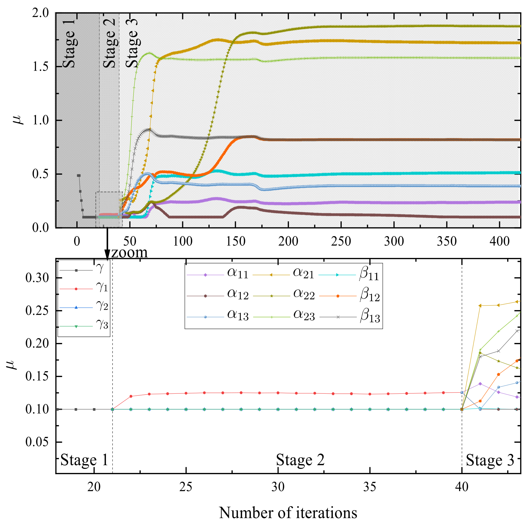
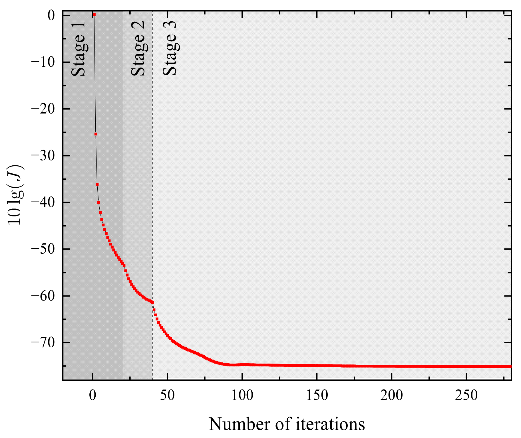
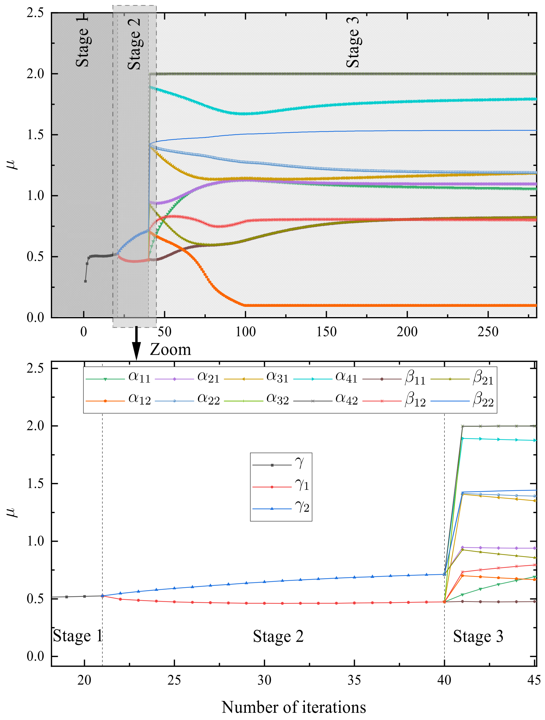
First, in Stage 1, $\mu \in ℝ$ is defined by Equation (15), its initial value is a one-dimensional random number. In each estimation subsystem ${\widehat{G}}_k(q)$, the estimated fractional-order vectors ${\widehat{\beta }}_k$ and ${\widehat{\alpha }}_k$ are solved as follows:

$${\widehat{\beta }}_k=\widehat{\mu }\left[\begin{array}{c}1\\ 2\\ ⋮\\ M_k\end{array}\right],{\widehat{\alpha }}_k=\widehat{\mu }\left[\begin{array}{c}1\\ 2\\ ⋮\\ N_k\end{array}\right],$$

(43)

where $\widehat{\mu }$ represents the estimated value of $\mu$. Based on the MILM algorithm, its iteration method is as follows:

$$\widehat{\mu }=\widehat{\mu }-{\left(J_{\mu }^{″}+\lambda I\right)}^{-1}{J}_{\mu }^{\prime },$$

(44)

where $J_{\mu }^{\prime }$ and $J_{\mu }^{″}$ are the gradient vector and Hessian matrix of the objective function $J(t)$ versus $\widehat{\mu }$, respectively, and their calculation method is as follows:

$$\begin{array}{c}{J}_{\mu }^{\prime }=-{\displaystyle \frac{2}{T}}\Xi (t,\mu ,L)E(t,\widehat{\theta },L)\\ J_{\mu }^{″}={\displaystyle \frac{2}{T}}\Xi (t,\mu ,L){\Xi }^{\mathrm{T}}(t,\mu ,L)\end{array}.$$

(45)

where

$$\Xi (t,\mu ,L)=[{\sigma }_{\widehat{y}(t)/\mu },{\sigma }_{\widehat{y}(t-h)/\mu },\cdots ,{\sigma }_{\widehat{y}(t-Lh+h)/\mu }]\in {ℝ}^{1\times L},$$

(46)

where ${\sigma }_{\widehat{y}(t)/\mu }$ represents the sensitivity function, which is calculated as follows:

$${\sigma }_{\widehat{y}(t)/\mu }={\displaystyle \frac{\widehat{y}(t,\widehat{\theta }\{\widehat{\mu }+d\mu \})-\widehat{y}(t,\widehat{\theta }\{\widehat{\mu }\})}{d\mu }}.$$

(47)

◆

Secondly, in Stage 2, $\mu \in {ℝ}^{K\times 1}$ is defined by Equation (17). Its initial value of $\mu$ is calculated as follows:

$$\mu ={\mu }^{Stage1}\cdot 1,$$

where ${\mu }^{Stage1}$ represents the convergence value of $\mu$ in Stage 1, and $1\in {ℝ}^{K\times 1}$ represents a vector with all elements equal to 1. In each estimation subsystem ${\widehat{G}}_k(q)$, the estimation fractional-order vectors ${\widehat{\beta }}_k$ and ${\widehat{\alpha }}_k$ are solved as follows:

$${\widehat{\beta }}_k={\widehat{\mu }}_k\left[\begin{array}{c}1\\ 2\\ ⋮\\ M_k\end{array}\right],{\widehat{\alpha }}_k={\widehat{\mu }}_k\left[\begin{array}{c}1\\ 2\\ ⋮\\ N_k\end{array}\right].$$

(48)

The sensitivity function ${\sigma }_{\widehat{y}(t)/\mu }$ is defined as follows:

$${\sigma }_{\widehat{y}(t)/\mu }=\left[\begin{array}{c}{\sigma }_{\widehat{y}(t)/{\mu }_1}\\ ⋮\\ {\sigma }_{\widehat{y}(t)/{\mu }_k}\\ ⋮\\ {\sigma }_{\widehat{y}(t)/{\mu }_K}\end{array}\right]\in {ℝ}^{K\times 1},$$

(49)

where the sensitivity function of each component ${\widehat{\mu }}_k$ in $\widehat{\mu }$ is calculated as

$${\sigma }_{\widehat{y}(t)/{\mu }_k}={\displaystyle \frac{\widehat{y}(t,\widehat{\theta }\{{\widehat{\mu }}_k+d\mu \})-\widehat{y}(t,\widehat{\theta }\{{\widehat{\mu }}_k\})}{d\mu }}.$$

(50)

◆

Finally, in Stage 3, $\mu \in {ℝ}^{{\displaystyle \sum _{k=1}^K\left(M_k+N_k\right)}\times 1}$ is defined by Equation (19). According to Equation (48), the initial value of $\mu$ calculation method is

$$\begin{array}{l}\mu =\left[{\mu }_1^{\mathrm{T}},{\mu }_2^{\mathrm{T}},\cdots ,{\mu }_K^{\mathrm{T}}\right]\\ {\mu }_k={\left[{\mu }_k^{Stage2}[1,2,\cdots ,M_k],{\mu }_k^{Stage2}[1,2,\cdots ,N_k]\right]}^{\mathrm{T}},\end{array}$$

where ${\mu }_k^{Stage2}$ represents the convergence value of the k-th element of the ${\mu }^{Stage2}$ vector in Stage 2. In each estimation subsystem ${\widehat{G}}_k(q)$, the estimation fractional order vectors ${\widehat{\beta }}_k$ and ${\widehat{\alpha }}_k$ are solved as follows:

$$\left\{\begin{array}{l}{\widehat{\beta }}_k={\widehat{\mu }}_k\{1:M_k\}\\ {\widehat{\alpha }}_k={\widehat{\mu }}_k\{\left[M_k+1\right]:\left[M_k+N_k\right]\}\end{array}\right..$$

(51)

The sensitivity function ${\sigma }_{\widehat{y}(t)/\mu }$ is defined as follows:

$${\sigma }_{\widehat{y}(t)/\mu }=\left[\begin{array}{c}{\sigma }_{\widehat{y}(t)/{\mu }_1}\\ ⋮\\ {\sigma }_{\widehat{y}(t)/{\mu }_i}\\ ⋮\\ {\sigma }_{\widehat{y}(t)/{\mu }_{{\displaystyle \sum _{k=1}^K\left(M_k+N_k\right)}}}\end{array}\right]\in {ℝ}^{{\displaystyle \sum _{k=1}^K\left(M_k+N_k\right)}\times 1},$$

(52)

where the sensitivity function of each component ${\widehat{\mu }}_i$ in $\widehat{\mu }$ is calculated as

$${\sigma }_{\widehat{y}(t)/{\mu }_i}={\displaystyle \frac{\widehat{y}(t,\widehat{\theta }\{{\widehat{\mu }}_i+d\mu \})-\widehat{y}(t,\widehat{\theta }\{{\widehat{\mu }}_i\})}{d\mu }}.$$

(53)

At this point, we have completed the introduction to the three-stage fractional-order identification method. In order to facilitate readers to understand and use the method in this article, combined with Section 3.1, we summarize the entire algorithm as follows:

Step 1: Initialize the estimated vectors $\widehat{\tilde{\chi }}$ and $\widehat{\mu }$, set the stage parameter $stage=1$, stage switching parameter $n_s=0$, harmonic coefficient $\lambda =1$, determine the stage switching threshold $N_s$, and determine the multi-innovation length $L$.

Step 2: Collect data $\left\{u_1(t),\cdots ,u_K(t),y^{*}(t)\right\}$ and decouple ${\widehat{\tilde{\chi }}}_k$ of each subsystem into ${\widehat{b}}_k$, ${\widehat{a}}_k$, and ${\widehat{p}}_k$ according to Equations (41) and (42). Solve $\widehat{\mu }$ into the fractional order vectors ${\widehat{\beta }}_k$ and ${\widehat{\alpha }}_k$ of each subsystem, where $k=1,\cdots K$, and the solution method is as follows:

$$\left\{\begin{array}{l}\mathrm{if} stage=1, \mathrm{in} \mathbf{Stage} 1, \mathrm{then} \mathrm{according} \mathrm{to} \mathrm{Equation} \left(43\right)\\ \mathrm{if} stage=2, \mathrm{in} \mathbf{Stage} 2, \mathrm{then} \mathrm{according} \mathrm{to} \mathrm{Equation} \left(48\right)\\ \mathrm{if} stage=3, \mathrm{in} \mathbf{Stage} 3, \mathrm{then} \mathrm{according} \mathrm{to} \mathrm{Equation} \left(51\right)\end{array}\right..$$

Step 3: The estimated output $\widehat{y}(t)$ is calculated according to Equations (20) and (21), $Y^{*}(t,\theta ,L)$ is calculated by Equation (37), and the multi-innovation output error vector $E(t,\theta )$ and the current objective function value $J(t)$ are calculated by Equations (32)–(34).

Step 4: If $J(t-h)<J(t)$, then increase $\lambda$, if else, decrease $\lambda$.

Step 5: If $\left|J(t)-J(t-h)\right|<\rho$, $\rho$ is a smaller value, then $n_s=n_s+1$, if else, continue.

Step 6: If $n_s>N_s$, then $n_s=0$, $stage=stage+1$, if else, continue.

Step 7: If $stage\ge 4\left|\right|J(t)<\zeta$, $\zeta$ is a smaller value, the estimation is completed and jumps to Step 9, if else, continue.

Step 8: Calculate $\Phi (t,\mu ,L)$ according to Equations (27), (30) and (38). Update $\widehat{\tilde{\chi }}$ and $\widehat{\mu }$ according to Equations (38) and (44). Then, go to Step 2.

Step 9: After the identification is completed, the estimated parameter $\widehat{\theta }$ is output according to Equation (11).

3.3. Computational Complexity Analysis

Under the assumption of equal iteration numbers, we compare the computational complexity of the staged and non-staged algorithms. We evaluate it by discussing the amount of matrix multiplication and addition, each counted as a floating-point operation. As the stage idea only serves for fractional-order parameter identification, the comparison focuses on the Step 2 related to the value of stage.

In each iteration, the statistics of the calculation amounts for the iteration of the fractional-order vector $\mu$ and the sensitivity function are presented as follows

Table 1. Calculation amount of equations for staged identification of fractional orders.

Stage	Equation	Calculation Amount	${\mathit{n}}_{\mathit{\mu }}(\mathit{s}\mathit{t}\mathit{a}\mathit{g}\mathit{e})$
1	Equation (44) Equation (47)	4	1
2	Equation (44) Equation (50)	$\left({\displaystyle \frac{8}{3}}{n}_{\mu }^3+{\displaystyle \frac{5}{2}}{n}_{\mu }^2+{\displaystyle \frac{17}{6}}{n}_{\mu }\right)$	$K$
3	Equation (44) Equation (53)		${\displaystyle \sum _{k=1}^K(N_k+M_k)}$

:

For non-staged identification, at the start of the identification process, it is the same as being in the final stage. Assume the total number of iterations is $N_{iter}$, and the number of iterations in each stage are $S_1$, $S_2$, $S_3$, respectively. Obviously $N_{iter}=S_1+S_2+S_3$.

The total calculation amount of the staged identification method is as follows:

$$\begin{array}{cc}\hfill C_1& =4S_1+\left({\displaystyle \frac{8}{3}}{n}_{\mu }^3(2)+{\displaystyle \frac{5}{2}}{n}_{\mu }^2(2)+{\displaystyle \frac{17}{6}}{n}_{\mu }(2)\right)S_2\hfill \\ & +\left({\displaystyle \frac{8}{3}}{n}_{\mu }^3(3)+{\displaystyle \frac{5}{2}}{n}_{\mu }^2(3)+{\displaystyle \frac{17}{6}}{n}_{\mu }(3)\right)S_3\hfill \end{array}.$$

(54)

The total calculation amount of the non-staged identification method is as follows:

$$C_2=\left({\displaystyle \frac{8}{3}}{n}_{\mu }^3(3)+{\displaystyle \frac{5}{2}}{n}_{\mu }^2(3)+{\displaystyle \frac{17}{6}}{n}_{\mu }(3)\right)N_{iter}$$

(55)

Subtracting Equation (55) from Equation (54), we can obtain

$$\begin{array}{ll}\hfill C_2-C_1=& -4S_1-\left({\displaystyle \frac{8}{3}}{n}_{\mu }^3(2)+{\displaystyle \frac{5}{2}}{n}_{\mu }^2(2)+{\displaystyle \frac{17}{6}}{n}_{\mu }(2)\right)S_2\hfill \\ & +\left({\displaystyle \frac{8}{3}}{n}_{\mu }^3(3)+{\displaystyle \frac{5}{2}}{n}_{\mu }^2(3)+{\displaystyle \frac{17}{6}}{n}_{\mu }(3)\right)\left(N_{iter}-S_3\right)\hfill \end{array}$$

(56)

By merging similar terms in Equation (56), we can obtain

$$\begin{array}{l}{C}_2-C_1=\left[\left({\displaystyle \frac{8}{3}}{n}_{\mu }^3(3)+{\displaystyle \frac{5}{2}}{n}_{\mu }^2(3)+{\displaystyle \frac{17}{6}}{n}_{\mu }(3)\right)-4\right]S_1\\ +\left[\begin{array}{c}{\displaystyle \frac{8}{3}}\left(n_{\mu }^3(3)-n_{\mu }^3(2)\right)+{\displaystyle \frac{5}{2}}\left(n_{\mu }^2(3)-n_{\mu }^2(2)\right)\\ +{\displaystyle \frac{17}{6}}\left(n_{\mu }(3)-n_{\mu }(2)\right)\end{array}\right]S_2\end{array}$$

(57)

Since $S_1>0$, $S_2>0$, $S_3>0$, $n_{\mu }(3)>n_{\mu }(2)>n_{\mu }(1)=1$, therefore $C_2-C_1>0$, $C_1<C_2$ according to Equation (57), and it can be seen that the staged MILM algorithm has a smaller computational workload.

4. Simulation Examples

In order to illustrate that the theory in this article is effective, we used the method in this article to identify the system parameters of an academic example system and a heat transfer system. The heat transfer system data came from Daisy [38]. The experimental details and results will be introduced next.

4.1. An Academic Example

In order to illustrate the reliability of the method, an academic example is used to simulate and verify the theory. Consider a non-homogeneous fractional-order Hammerstein MISO system with structural parameters $N_k=2$, $M_k=1$, $Q_k=2$, $k=1,\cdots ,K$ and the number of input signals $K=3$ as follows:

$$\left\{\begin{array}{l}{\overline{u}}_1(t)=0.5{\left[u_1(t)\right]}^2+\left[u_1(t)\right]\\ {\overline{u}}_2(t)=0.3{\left[u_2(t)\right]}^2+\left[u_2(t)\right]\\ {\overline{u}}_3(t)=0.8{\left[u_3(t)\right]}^2+\left[u_3(t)\right]\\ y_1(t)={\displaystyle \frac{1+q^{0.5}}{1.9q^{0.2}+0.5q^{1.7}}}{\overline{u}}_1(t)\\ y_2(t)={\displaystyle \frac{0.5+0.6s^{0.8}}{1.9q^{0.1}+0.4q^{1.9}}}{\overline{u}}_2(t)\\ y_3(t)={\displaystyle \frac{1.5+2s^{0.8}}{1.3q^{0.4}+0.6q^{1.6}}}{\overline{u}}_3(t)\\ y(t)={\displaystyle \sum _{k=1}^3{y}_k}(t)\\ y^{*}(t)=y(t)+v(t)\end{array}\right.$$

where the system input $u(t)$ is selected as a Gaussian random sequence with a mean of 0 and a variance of 1. The sampling time is 1 s. The total running time is 1000 s. The noise $v(t)$ is considered to be Gaussian white noise with a mean value of 0, and its variance is determined by the signal-to-noise ratio (SNR). It is defined as follows:

$$\mathrm{var}(v)={10}^{-{\displaystyle \frac{SNR}{10}}}.$$

During the parameter identification process, the system structure is determined as a priori knowledge. The identification is based on the collected data $\left\{u_1(t),u_2(t),u_3(t),y^{*}(t)\right\}$. The experiment carried out 100 Monte Carlo parameter identification experiments. In the experiment, the system noise $v(t)$ and initial parameter values were random, and the innovation length $L=\left\{1,3,5\right\}$ was set, respectively. First, the statistical box plot of the final value of the objective function $J(t)$ under different innovation lengths is given.

As can be seen from Figure 2, in the same innovation length, the identification effect of the algorithm is basically the same for different signal-to-noise ratios, which reflects the stability of the algorithm. When the innovation length of the algorithm increases to a limited extent, under different signal-to-noise ratios, the statistical mean and median line of the convergence value of the objective function are significantly reduced. This proves that the introduction of multi-innovation theory enhances the convergence accuracy of classic LM and improves the performance of the algorithm.

Table 2. Statistics of parameter identification results of $G_1(q)$ in the experiment (L = 5).

Ture	Estimates (SNR = 25 dB)	Estimates (SNR = 34 dB)
$b_{0,1}=1$	0.954041 ± 0.04224	0.963504 ± 0.00318
$b_{1,1}=1$	1.1 ± 0.00001	1.1 ± 0.00001
$a_{1,1}=1.9$	2 ± 0.00001	1.9985 ± 0.04019
$a_{2,1}=0.5$	0.490984 ± 0.0276	0.504801 ± 0.00502
$p_{1,1}=0.5$	0.500751 ± 0.000648	0.0500529 ± 0.00004
$p_{2,1}=1$	1	1
${\beta }_{1,1}=0.5$	0.488174 ± 0.004843	0.495444 ± 0.00246
${\alpha }_{1,1}=0.2$	0.1800045 ± 0.001908	0.223436 ± 0.000645
${\alpha }_{2,1}=1.7$	1.735957 ± 0.029478	1.723453 ± 0.004743
$b_{0,2}=0.5$	0.475162 ± 0.011939	0.477988 ± 0.00368
$b_{1,2}=0.6$	0.594816 ± 0.01381	0.589707 ± 0.004302
$a_{1,2}=1.9$	1.800045 ± 0.001908	1.800448 ± 0.001315
$a_{2,2}=0.4$	0.40967 ± 0.013693	0.402033 ± 0.005661
$p_{1,2}=0.3$	0.300015 ± 0.0002	0.299971 ± 0.00001
$p_{2,2}=1$	1	1
${\beta }_{1,2}=0.8$	0.813024 ± 0.00671	0.809725 ± 0.003573
${\alpha }_{1,2}=0.1$	0.114096 ± 0.01612	0.110667 ± 0.004548
${\alpha }_{2,2}=1.9$	1.874833 ± 0.01404	1.883352 ± 0.00602
$b_{0,3}=1.5$	1.499388 ± 0.11051	1.497258 ± 0.002258
$b_{1,3}=2$	1.906755 ± 0.00676	1.906323 ± 0.00207
$a_{1,3}=1.3$	1.2068 ± 0.006935	1.206316 ± 0.001229
$a_{2,3}=0.6$	0.615202 ± 0.006313	0.613663 ± 0.000871
$p_{1,3}=0.8$	0.799962 ± 0.00676	0.799991 ± 0.00001
$p_{2,3}=1$	1	1
${\beta }_{1,3}=0.8$	0.817697 ± 0.00432	0.817434 ± 0.000618
${\alpha }_{1,3}=0.4$	0.388925 ± 0.00782	0.390009 ± 0.00177
${\alpha }_{2,3}=1.6$	1.580773 ± 0.00448	1.581597 ± 0.00122

shows the statistical results of parameter identification of 100 Monte Carlo experiments under different signal-to-noise ratios of the algorithm. Table 2 is split into three parts, which, respectively, show the input-related parameters of each system, including the coefficients and fractional orders of the fractional transfer function, as well as the coefficients of the nonlinear part. It can be seen that under different signal-to-noise ratios, statistical data show that as the number of multiple innovations increases, the value of the final objective function becomes smaller, which proves that the introduction of the multiple innovation theory is effective.

Figure 3 shows the change curves of the fractional order of the estimated system in the three stages of the entire identification process. Among them, the stage switching process of the estimated fractional-order system is partially enlarged and displayed. The number of fractional orders continues to increase as the stage increases. Finally, in Stage 3, its number is consistent with the number of the original system, and the algorithm also reaches convergence in Stage 3. It can be seen that only one one-dimensional fractional-order initial value is specified in the entire identification process, and the fractional-order vectors in the subsequent stages are all “split” from the fractional-order initial value, which reduces the difficulty of initializing the fractional-order parameters. Moreover, as can be seen from the analysis in 3.3, this also reduces the computational complexity of the early algorithm in the identification process.

4.2. Heat Flow Density Through a Two Layers Wall System Modeling

This section conducts fractional-order system modeling of heat flow density through a two layers wall system to verify the practicability of the algorithm. The system contains two inputs and one output. The heat flow flows from the inner wall surface to the outer wall surface, and the intermediate heat flux density is used as the output of the system. These data come from the DAISY database [34], with a total of 1680 groups, provided by the ESAT/SISTA electrical department. These data record the heat flux through two layers of wall (brick wall and insulation material), where the input sequence includes the inner wall temperature $u_1$ and the outer wall temperature $u_2$, and the output sequence is the heat flux density $y$. It is normalized and Gaussian smoothed, and the data are obtained as shown in Figure 4.

Different from the academic example in Section 4.1, the system structure of the actual system is not known a priori. The experiment needs to determine the system structure to ensure the accuracy of the identification model. The system structure vector is represented as

$$[N,M,Q],$$

where the transfer function structure $N=N_k,M=M_k,k=1,\cdots ,K$ and the polynomial order $Q=Q_k,k=1,\cdots ,K$ are included.

In this part of the work, we chose to learn from the existing work [30], tested a total of 64 system structures from $[2,2,2]$ to $[5,5,5]$, eliminated poor results, and counted the objective function values of the identification results under different system structures in Figure 5. It can be seen from the results that when the system structure is $[4,2,4]$, the experimental objective function value is the smallest at this time. Therefore, the $[4,2,4]$ structure is adopted as the structure of the non-homogeneous fractional-order Hammerstein MISO system. According to Equation (11), the unknown system and parameter vector to be identified can be expressed as follows:

$$\left\{\begin{array}{l}{\overline{u}}_1(t)=p_{1,1}{\left[u_1(t)\right]}^4+p_{2,1}{\left[u_1(t)\right]}^3+p_{3,1}{\left[u_1(t)\right]}^2+\left[u_1(t)\right]\\ {\overline{u}}_2(t)=p_{1,2}{\left[u_2(t)\right]}^4+p_{2,2}{\left[u_2(t)\right]}^3+p_{3,2}{\left[u_2(t)\right]}^2+\left[u_2(t)\right]\\ y_1(t)={\displaystyle \frac{b_{0,1}+b_{1,1}{q}^{{\beta }_{1,1}}+b_{2,1}{q}^{{\beta }_{2,1}}}{a_{1,1}{q}^{{\alpha }_{1,1}}+a_{2,1}{q}^{{\alpha }_{2,1}}+a_{3,1}{q}^{{\alpha }_{3,1}}+a_{4,1}{q}^{{\alpha }_{4,1}}}}{\overline{u}}_1(t)\\ y_2(t)={\displaystyle \frac{b_{0,2}+b_{1,2}{s}^{{\beta }_{1,2}}+b_{2,2}{s}^{{\beta }_{2,2}}}{a_{1,2}{q}^{{\alpha }_{1,2}}+a_{2,2}{q}^{{\alpha }_{2,2}}+a_{3,2}{q}^{{\alpha }_{3,2}}+a_{4,2}{q}^{{\alpha }_{4,2}}}}{\overline{u}}_2(t)\\ y(t)=y_1(t)+y_2(t)\end{array}\right.,$$

$$\theta ={\left[b_1^{\mathrm{T}},a_1^{\mathrm{T}},b_2^{\mathrm{T}},a_2^{\mathrm{T}},p_1^{\mathrm{T}},p_2^{\mathrm{T}},{\beta }_1^{\mathrm{T}},{\alpha }_1^{\mathrm{T}},{\beta }_2^{\mathrm{T}},{\alpha }_2^{\mathrm{T}}\right]}^{\mathrm{T}}\in {ℝ}^{34\times 1},$$

$$\begin{array}{l}{b}_1={\left[b_{0,1},b_{1,1},b_{2,1}\right]}^{\mathrm{T}}\in {ℝ}^{3\times 1}\\ a_1={\left[a_{1,1},a_{2,1},a_{3,1},a_{4,1}\right]}^{\mathrm{T}}\in {ℝ}^{4\times 1}\\ b_2={\left[b_{0,2},b_{1,2},b_{2,2}\right]}^{\mathrm{T}}\in {ℝ}^{3\times 1}\\ a_2={\left[a_{1,2},a_{2,2},a_{3,2},a_{4,2}\right]}^{\mathrm{T}}\in {ℝ}^{4\times 1},\end{array}$$

$$\begin{array}{l}{p}_1={\left[p_{1,1},p_{2,1},p_{3,1},p_{4,1}\right]}^{\mathrm{T}}\in {ℝ}^{4\times 1}\\ p_2={\left[p_{1,2},p_{2,2},p_{3,2},p_{4,2}\right]}^{\mathrm{T}}\in {ℝ}^{4\times 1},\end{array}$$

$$\begin{array}{l}{\beta }_1={\left[{\beta }_{1,1},{\beta }_{2,1}\right]}^{\mathrm{T}}\in {ℝ}^{2\times 1}\\ {\alpha }_1={\left[{\alpha }_{1,1},{\alpha }_{2,1},{\alpha }_{3,1},{\alpha }_{4,1}\right]}^{\mathrm{T}}\in {ℝ}^{4\times 1}\\ {\beta }_2={\left[{\beta }_{1,2},{\beta }_{2,2}\right]}^{\mathrm{T}}\in {ℝ}^{2\times 1}\\ {\alpha }_2={\left[{\alpha }_{1,2},{\alpha }_{2,2},{\alpha }_{3,2},{\alpha }_{4,2}\right]}^{\mathrm{T}}\in {ℝ}^{4\times 1}.\end{array}$$

Using the algorithm in this article to identify unknown parameters, the following non-homogeneous fractional-order Hammerstein MISO system can be obtained.

$$\left\{\begin{array}{l}{\overline{u}}_1(t)=-0.1050{\left[u_1(t)\right]}^4+0.0127{\left[u_1(t)\right]}^3+0.0878{\left[u_1(t)\right]}^2+\left[u_1(t)\right]\\ {\overline{u}}_2(t)=0.0352{\left[u_2(t)\right]}^4-0.0347{\left[u_2(t)\right]}^3-0.0381{\left[u_2(t)\right]}^2+\left[u_1(t)\right]\\ y_1(t)={\displaystyle \frac{-0.9387+0.7272q^{0.8318}+0.5432q^{0.8318}}{2.2996q^{1.0356}+1.9526q^{1.0992}+2.0037q^{1.2246}+0.7807q^{1.8148}}}{\overline{u}}_1(t)\\ y_2(t)={\displaystyle \frac{0.8758+1.3698q^{0.7979}+0.1468q^{1.5384}}{1.0081q^{0.1003}+0.7059q^{1.1839}-0.0282q^2-0.0242q^2}}{\overline{u}}_2(t)\\ y(t)=y_1(t)+y_2(t)\end{array}\right..$$

Figure 6 shows the decline curve of the objective function during the identification process. It can be seen that the objective function value continues to decrease with the number of iterations of the algorithm and tends to converge. During the convergence process, the convergence curve decreases in three stages, and there is an obvious turning point at the switching point between adjacent stages. This is caused by the fractional order quantity switching of the system to be identified. In the specific identification process, the fractional order change curve is presented in Figure 7. It can be seen that from Stage 1 to Stage 3, the system grows from a global homogeneous fractional-order system to a local homogeneous fractional-order system, and finally splits and changes into a non-homogeneous fractional-order system. In this process, the fractional order starts with a one-dimensional number and the dimension grows as the algorithm runs. This is particularly useful for fractional-order systems with a large number of fractional orders. Figure 6 shows a partial enlargement of the fractional order quantity change process in the three stages.

Figure 8 gives the comparison between the estimated output of the estimated system and the output of the real system. It can be seen that the estimated system output and the real system output curve basically coincide, which proves the practicability of the algorithm.

To further illustrate the advantages of the algorithm, we compare the estimated system output and actual system output error MSE with [34], and the results are shown in

Table 3. Algorithm comparison results.

	[34]	This Paper
MSE	2.55 × 10−2	5.47 × 10−4

. It can be seen that compared with [34], the method proposed in this paper has higher fitting accuracy, which proves the superiority of our method.

5. Conclusions

This paper proposes an LM algorithm based on the multi-innovation principle for parameter identification of non-homogeneous fractional-order Hammerstein MISO systems. The fractional-order identification process is split into three stages, and different stages correspond to different numbers of fractional orders to be identified. The algorithm is verified in two experiments. The conclusion is summarized as follows:

1. For a non-homogeneous fractional-order Hammerstein MISO system, the algorithm can effectively identify the parameters. Under different signal-to-noise ratios, the algorithms show relatively stable performance. Through Monte Carlo experiments, we concluded that with a limited increase in the number of innovations, the convergence accuracy of the algorithm will improve, which confirms the effectiveness of the multi-innovation theory.

2. The identification of fractional orders ranges from simple to complex. The algorithm provides an automatic selection method for the initial value of the identification of fractional orders in system identification work for non-homogeneous fractional-order Hammerstein systems. This theory plays an important role in modeling non-homogeneous fractional orders of complex actual systems. The three-stage modeling process of fractional-order identification can be clearly captured in the convergence curve. As the dimensions of the fractional order vectors to be estimated in the three stages increase, the algorithm can calculate feasible non-homogeneous fractional-order Hammerstein MISO systems to describe practical problems, and the practicability of the algorithm has been verified.

In subsequent work, we will extend the method in this article to MIMO systems and optimize the gradient calculation of the fractional-order identification process.

References

- Salman, I.; Lin, Y.A.N.; Hamayun, M.T. Fractional order modeling and control of dissimilar redundant actuating system used in large passenger aircraft. Chin. J. Aeronaut. 2018, 31, 1141–1152. [Google Scholar]
- Li, L.; Yu, X.; Jiang, Q.; Zang, B.; Jiang, L. Synchrosqueezing transform meets α-stable distribution: An adaptive fractional lower-order SST for instantaneous frequency estimation and non-stationary signal recovery. Signal Process. 2022, 201, 108683. [Google Scholar] [CrossRef]
- Singh, J.; Kumar, D.; Kumar, S. An efficient computational method for local fractional transport equation occurring in fractal porous media. Comput. Appl. Math. 2020, 39, 137. [Google Scholar] [CrossRef]
- Dirlik, T.; Benasciutti, D. Dirlik and tovo-benasciutti spectral methods in vibration fatigue: A review with a historical perspective. Metals 2021, 11, 1333. [Google Scholar] [CrossRef]
- Bingi, K.; Prusty, B.R. Forecasting models for chaotic fractional-order oscillators using neural networks. Int. J. Appl. Math. Comput. Sci. 2021, 31, 387–398. [Google Scholar] [CrossRef]
- Patil, M.D.; Vadirajacharya, K.; Khubalkar, S.W. Design and tuning of digital fractional-order PID controller for permanent magnet DC motor. IETE J. Res. 2023, 69, 4349–4359. [Google Scholar] [CrossRef]
- Qiao, Z.; Elhattab, A.; Shu, X.; He, C. A second-order stochastic resonance method enhanced by fractional-order derivative for mechanical fault detection. Nonlinear Dyn. 2021, 106, 707–723. [Google Scholar] [CrossRef]
- Gong, P.; Lan, W.; Han, Q.L. Robust adaptive fault-tolerant consensus control for uncertain nonlinear fractional-order multi-agent systems with directed topologies. Automatica 2020, 117, 109011. [Google Scholar] [CrossRef]
- Wu, J.X.; Chen, P.Y.; Li, C.M.; Kuo, Y.C.; Pai, N.S.; Lin, C.H. Multilayer fractional-order machine vision classifier for rapid typical lung diseases screening on digital chest X-ray images. IEEE Access 2020, 8, 105886–105902. [Google Scholar] [CrossRef]
- Li, P.; Xiong, L.; Wang, Z.; Ma, M.; Wang, J. Fractional-order sliding mode control for damping of subsynchronous control interaction in DFIG-based wind farms. Wind Energy 2020, 23, 749–762. [Google Scholar] [CrossRef]
- Zhang, T.; Zhou, J.; Liao, Y. Exponentially stable periodic oscillation and Mittag–Leffler stabilization for fractional-order impulsive control neural networks with piecewise Caputo derivatives. IEEE Trans. Cybern. 2021, 52, 9670–9683. [Google Scholar] [CrossRef] [PubMed]
- Elwy, O.; Said, L.A.; Madian, A.H.; Radwan, A.G. All possible topologies of the fractional-order Wien oscillator family using different approximation techniques. Circuits Syst. Signal Process. 2019, 38, 3931–3951. [Google Scholar] [CrossRef]
- Zhang, Q.; Wang, H.; Liu, C. Identification of fractional-order Hammerstein nonlinear ARMAX system with colored noise. Nonlinear Dyn. 2021, 106, 3215–3230. [Google Scholar] [CrossRef]
- Sun, M.; Wang, H.; Zhang, Q. Identification of fractional order Hammerstein models based on mixed signals. J. Control. Decis. 2022, 11, 132–138. [Google Scholar] [CrossRef]
- Laribi, S.; Mammar, K.; Sahli, Y.; Necaibia, A.; Arama, F.Z.; Ghaitaoui, T. PEMFC water diagnosis using PWM functionality signal and fractional order model. Energy Rep. 2021, 7, 4214–4221. [Google Scholar] [CrossRef]
- AbouOmar, M.S.; Zhang, H.J.; Su, Y.X. Fractional order fuzzy PID control of automotive PEM fuel cell air feed system using neural network optimization algorithm. Energies 2019, 12, 1435. [Google Scholar] [CrossRef]
- Chen, L.; Yin, H.; Huang, T.; Yuan, L.; Zheng, S.; Yin, L. Chaos in fractional-order discrete neural networks with application to image encryption. Neural Netw. 2020, 125, 174–184. [Google Scholar] [CrossRef]
- Li, Y.; Huang, M.; Li, B. Besicovitch almost periodic solutions for fractional-order quaternion-valued neural networks with discrete and distributed delays. Math. Methods Appl. Sci. 2022, 45, 4791–4808. [Google Scholar] [CrossRef]
- Buscarino, A.; Caponetto, R.; Graziani, S.; Murgano, E. Realization of fractional order circuits by a Constant Phase Element. Eur. J. Control 2020, 54, 64–72. [Google Scholar] [CrossRef]
- Zhang, L.; Chen, X.; Xu, Y.; Jin, M.; Ye, X.; Gao, H.; Chu, W.; Mao, J.; Thompson, M.L. Soil labile organic carbon fractions and soil enzyme activities after 10 years of continuous fertilization and wheat residue incorporation. Sci. Rep. 2020, 10, 11318. [Google Scholar] [CrossRef]
- Yamni, M.; Karmouni, H.; Sayyouri, M.; Qjidaa, H. Robust audio watermarking scheme based on fractional Charlier moment transform and dual tree complex wavelet transform. Expert Syst. Appl. 2022, 203, 117325. [Google Scholar] [CrossRef]
- Babu, N.R.; Kalpana, M.; Balasubramaniam, P. A novel audio encryption approach via finite-time synchronization of fractional order hyperchaotic system. Multimed. Tools Appl. 2021, 80, 18043–18067. [Google Scholar] [CrossRef]
- Qian, Z.; Hongwei, W.; Chunlei, L. Hybrid identification method for fractional-order nonlinear systems based on the multi-innovation principle. Appl. Intell. 2023, 53, 15711–15726. [Google Scholar] [CrossRef]
- Zhang, Q.; Wang, H.; Liu, C. MILM hybrid identification method of fractional order neural-fuzzy Hammerstein model. Nonlinear Dyn. 2022, 108, 2337–2351. [Google Scholar] [CrossRef]
- Qian, Z.; Hongwei, W.; Chunlei, L.; Xiaojing, M. Multi-innovation identification method for fractional Hammerstein state space model with colored noise. Chaos Solitons Fractals 2023, 173, 113631. [Google Scholar] [CrossRef]
- Victor, S.; Malti, R.; Garnier, H.; Oustaloup, A. Parameter and differentiation order estimation in fractional models. Automatica 2013, 49, 926–935. [Google Scholar] [CrossRef]
- Mayoufi, A.; Victor, S.; Chetoui, M.; Malti, R.; Aoun, M. Output Error MISO System Identification Using Fractional Models. Fract. Calc. Appl. Anal. 2021, 24, 1601–1618. [Google Scholar] [CrossRef]
- Victor, S.; Mayoufi, A.; Malti, R.; Chetoui, M.; Aoun, M. System identification of MISO fractional systems: Parameter and differentiation order estimation. Automatica 2022, 141, 110268. [Google Scholar] [CrossRef]
- Liu, C.; Wang, H.; Zhang, Q.; Ma, X. Online identification of non-homogeneous fractional order Hammerstein continuous systems based on the principle of multi-innovation. Nonlinear Dyn. 2023, 111, 20111–20125. [Google Scholar] [CrossRef]
- Can, N.H.; Nikan, O.; Rasoulizadeh, M.N.; Jafari, H.; Gasimov, Y.S. Numerical computation of the time non-linear fractional generalized equal width model arising in shallow water channel. Therm. Sci. 2020, 24, 49–58. [Google Scholar] [CrossRef]
- Jafari, H.; Ganji, R.M.; Ganji, D.D.; Hammouch, Z.; Gasimov, Y.S. A novel numerical method for solving fuzzy variable-order differential equations with Mittag-Leffler kernels. Fractals 2023, 31, 2340063. [Google Scholar] [CrossRef]
- Boutiba, M.; Baghli-Bendimerad, S.; El Houda Bouzara-Sahraoui, N. Numerical solution by finite element method for time Caputo-Fabrizio fractional partial diffusion equation. Adv. Math. Models Appl. 2024, 9, 316–328. [Google Scholar]
- Narsale, S.M.; Lodhi, R.K.; Jafari, H. A numerical study for non-linear multi-term fractional order differential equations. Adv. Math. Models Appl. 2024, 9, 193–204. [Google Scholar]
- Liu, C.; Wang, H.; Zhang, Q.; Ahemaide, M. Identification of fractional order non– homogeneous Hammerstein-Wiener MISO continuous systems. Mech. Syst. Signal Process. 2023, 197, 110400. [Google Scholar]
- Matignon, D. Stability properties for generalized fractional differential systems. EDP Sci. 1998, 5, 145–158. [Google Scholar] [CrossRef]
- Hammar, K.; Djamah, T.; Bettayeb, M. Nonlinear system identification using fractional Hammerstein–Wiener models. Nonlinear Dyn. 2019, 98, 2327–2338. [Google Scholar] [CrossRef]
- Wang, Z.; Wang, C.; Ding, L.; Wang, Z.; Liang, S. Parameter identification of fractional-order time delay system based on Legendre wavelet. Mech. Syst. Signal Process. 2022, 163, 108141. [Google Scholar] [CrossRef]
- De Moor, B.; De Gersem, P.; De Schutter, B.; Favoreel, W. DAISY: A database for identification of systems. J. A 1997, 38, 5. [Google Scholar]