A POD-Based Reduced-Dimension Method for Solution Coefficient Vectors in the Crank–Nicolson Mixed Finite Element Method for the Fourth-Order Parabolic Equation

Abstract

This research proposes a method for reducing the dimension of the coefficient vector for Crank–Nicolson mixed finite element (CNMFE) solutions to solve the fourth-order variable coefficient parabolic equation. Initially, the CNMFE schemes and corresponding matrix schemes for the equation are established, followed by a thorough discussion of the uniqueness, stability, and error estimates for the CNMFE solutions. Next, a matrix-form reduced-dimension CNMFE (RDCNMFE) method is developed utilizing proper orthogonal decomposition (POD) technology, with an in-depth discussion of the uniqueness, stability, and error estimates of the RDCNMFE solutions. The reduced-dimension method employs identical basis functions, unlike standard CNMFE methods. It significantly reduces the number of unknowns in the computations, thereby effectively decreasing computational time, while there is no loss of accuracy. Finally, numerical experiments are performed for both fourth-order and time-fractional fourth-order parabolic equations. The proposed method demonstrates its effectiveness not only for the fourth-order parabolic equations but also for time-fractional fourth-order parabolic equations, which further validate the universal applicability of the POD-based RDCNMFE method. Under a spatial discretization grid $40\times 40$, the traditional CNMFE method requires $2\times {41}^2$ degrees of freedom at each time step, while the RDCNMFE method reduces the degrees of freedom to $2\times 6$ through POD technology. The numerical results show that the RDCNMFE method is nearly 10 times faster than the traditional method. This clearly demonstrates the significant advantage of the RDCNMFE method in saving computational resources.

1. Introduction

This research focuses on exploring the fourth-order variable coefficient parabolic equation with the initial-boundary value

$$\begin{array}{c}\hfill \left\{\begin{array}{cc}{u}_t+\epsilon \nabla ·(b(\mathit{x},t)\nabla (\nabla ·(a(t)\nabla u)))=f(u),\hfill & (\mathit{x},t)\in \Omega \times J,\hfill \\ u(\mathit{x},t)=\Delta u(\mathit{x},t)=0,\hfill & (\mathit{x},t)\in \partial \Omega \times \overline{J},\hfill \\ u(\mathit{x},0)=u_0(\mathit{x}),\hfill & \mathit{x}\in \Omega .\hfill \end{array}\right.\end{array}$$

(1)

$\Omega \subset {\mathbb{R}}^d(d=1,2,3)$ is a bounded convex polygonal domain. $\partial \Omega$ is a boundary of $\Omega$. $J=(0,T],0<T<\infty$. $u_0(\mathit{x})$ is a known initial function. $a=a(t)$, $b=b(\mathit{x},t)$ satisfying

$$\begin{array}{c}{\mathbf{H}}_1:0<a_0⩽a(t)⩽a_1<+\infty ,\hfill \\ {\mathbf{H}}_2:0<b_0⩽b(\mathit{x},t)⩽b_1<+\infty ,\hfill \\ {\mathbf{H}}_3:|a_t(t)|+|b_t(\mathit{x},t)|⩽d_0,\hfill \end{array}$$

(2)

for some positive constants, $a_0$, $a_1$, $b_0$, $b_1$, and $d_0$. $\epsilon$ is a positive constant. $f(u)=u^3-u$ satisfies the following properties

$$\left|f(u)\right|⩽|u{|}^3+|u|.$$

(3)

For simplicity, we assume that $u_0(\mathit{x})=0$ in the following theoretical analysis.

The fourth-order parabolic equations are commonly used to describe higher-order physical behaviors, such as considering the internal damping or viscoelastic properties of materials. Within the category of fourth-order parabolic equations, models such as the Cahn—Hilliard equation [1,2], the fourth-order reaction–diffusion equation [3,4], and the Swift–Hohenberg equation [5] are included. Due to the inclusion of higher-order derivatives, solving and analyzing these kinds of equations is usually more complex and often requires the use of numerical methods. Currently, a range of numerical methods are applied to address fourth-order parabolic equations, for example, the finite element (FE) method [1,6,7], mixed finite element method (MFE) [3,8,9,10], discontinuous space–time MFE method [11,12], two-grid MFE method [13,14], weak Galerkin FE method [2,15], finite difference method [16], implicit compact difference method [17,18,19,20], cubic spline method [21], blow-up method [22,23,24,25], and so on. In this paper, the MFE method is employed to study the fourth-order variable coefficient parabolic equation for spatial analysis. The Crank–Nicolson (CN) scheme is used for time discretization.

A prevalent challenge in addressing high-order partial differential equations (PDEs) through the MFE method is the rapid escalation of unknown dimensions when dealing with coupled equations, often resulting in a doubling of the data volume processed. Such significantly elevated dimensions not only heighten memory requirements but also substantially escalate computational costs. In practical scenarios, this increased computational burden can pose a significant barrier to solving complex PDE problems. An effective strategy for mitigating these challenges involves the implementation of order reduction techniques. The primary objective of these techniques is to minimize the number of variables considered during the solution process using mathematical methods, thereby alleviating computational demands while preserving as much as possible a good approximation quality. Currently, several effective numerical reduced-order methods have gained widespread application, including the POD method [26,27], the spectral element method [28], the sparse grid method [29], and the balanced truncation method [30].

Certainly, integrating POD technology with diverse numerical methods can effectively address a range of PDEs. It is the most widely utilized method for dimensionality reduction, and it has been attracting increasing attention. Refs [31,32] combined the compact difference method and POD technique to study the fourth-order parabolic equation. Zhao and Piao [33] studied the KDV-RLW-Rosenau equation using the POD method in conjunction with B-spline Galerkin FE formulations. In [34], the heat equation was addressed using the POD reduced-order methods and the two-step backward differentiation formula (BDF2). Janes and Singler [35] solved the damped wave equation through the POD method and second difference quotients (DDQs). He et al. [36] employed a space-time FE method that integrates a POD-based extrapolation with DG time stepping to analyze the parabolic equation. Lu et al. [37] merged the POD method with a collocation approach using local radial basis functions (RBFs) to address time-dependent nonlocal diffusion problems.

For the POD-based FE and MFE reduced-dimension models, there are two existing methods. The first involves establishing optimized models that reduce the dimensions of the FE or the MFE subspaces. For further references, please consult [38,39,40,41,42,43,44]. The second, introduced by Luo et al. in 2020, presents an innovative strategy for the dimension reduction in CNFE [45,46] and CNMFE [47,48,49,50,51] solution coefficient vectors. To our understanding, no existing literature has documented simplifying the solution coefficient vectors of CNMFE scheme using POD technology in solving fourth-order variable coefficient parabolic equations. This paper’s primary objective is to present a rapid algorithm capable of solving fourth-order variable coefficient parabolic equations. Since the proposed methods prove to be computationally effective for both fourth-order and time-fractional fourth-order parabolic equations, we naturally extend their application to time-fractional fourth-order parabolic equations. For the time-fractional derivative term ${\displaystyle \frac{{\partial }^{\alpha }u}{\partial t^{\alpha }}}$, we employ the Caputo derivative, defined as

$${\displaystyle \frac{{\partial }^{\alpha }u(x,t)}{\partial t^{\alpha }}}={\displaystyle \frac{1}{\Gamma (1-\alpha )}}{\int }_0^t{\displaystyle \frac{\partial u(x,\tau )}{\partial \tau }}{\displaystyle \frac{d\tau }{{(t-\tau )}^{\alpha }}},0<\alpha <1.$$

(4)

This research is organized as follows: Section 2 discusses the CNMFE scheme, detailing its uniqueness, stability, and convergence. Section 3 is dedicated to constructing a POD-based RDCNMFE matrix model while also analyzing its uniqueness, stability, and error estimates. In Section 4, we perform numerical simulations on 2D fourth-order and time-fractional fourth-order variable coefficient parabolic equations, respectively. Finally, Section 5 summarizes the key results and conclusions of the research.

2. The CNMFE Method for the Fourth-Order Variable Coefficient Parabolic Equation

2.1. The CNMFE Scheme

In this paper, the Sobolev spaces and the associated norms adhere to the conventional definitions commonly found in the existing literature [52]. To construct the CNMFE scheme for the fourth-order variable coefficient parabolic Equation (1), we begin by introducing a diffusion term defined as $q=-\nabla ·(a(t)\nabla u)$. This introduces a pair of lower-order equations

$$\left\{\begin{array}{c}{u}_t-\epsilon \nabla ·(b(\mathit{x},t)\nabla q)=f(u),(\mathit{x},t)\in \Omega \times J,\hfill \\ q+\nabla ·(a(t)\nabla u)=0,(\mathit{x},t)\in \Omega \times J,\hfill \\ u(\mathit{x},t)=q(\mathit{x},t)=0,(\mathit{x},t)\in \partial \Omega \times \overline{J}.\hfill \end{array}\right.$$

(5)

Utilizing Green’s integration formula in the variational framework leads to the weak mixed formulation of (5), which is explicitly constructed below.

Problem 1.

Find $\{u,q\}$: $[0,T]\mapsto H_0^1\times H_0^1$, such that

$$\begin{array}{c}\hfill \left\{\begin{array}{c}(u_t,\upsilon )+\epsilon (b\nabla q,\nabla \upsilon )=(f(u),\upsilon ),\forall \upsilon \in H_0^1,\hfill \\ (q,\chi )-(a\nabla u,\nabla \chi )=0,\forall \chi \in H_0^1,\hfill \end{array}\right.\end{array}$$

(6)

Given a quasi-uniform triangulation, ${\Im }_h$ on $\overline{\Omega }$, the finite element subspace ${\mathbb{S}}_h$ is spanned by the following orthonormal basis ${\left\{{\zeta }_j(x)\right\}}_{j=1}^M$

$$\begin{array}{c}{\mathbb{S}}_h=\{{\upsilon }_h\in H_0^1\cap C(\Omega );{\upsilon }_h{\mid }_K\in {\mathbb{P}}_{M-1}(K),K\in \Im \}=\mathrm{span}\{{\zeta }_j(\mathit{x}):1⩽j⩽M\},\hfill \end{array}$$

(7)

where ${\mathbb{P}}_{M-1}(K)$ is a polynomial space of $(M-1)$ degree, M is the dimension of the space ${\mathbb{S}}_h$, and ${\left\{{\zeta }_i\right\}}_{i=1}^M$ satisfies

$$({\zeta }_i,{\zeta }_j)={\delta }_{ij}=\left\{\begin{array}{cc}1,\hfill & i=j,\hfill \\ 0,\hfill & i\ne j,\hfill \end{array}\right.i,j=1,2,\cdots ,M.$$

For a positive integer, N, define $\Delta t=T/N$, ${\psi }^n=\psi (t_n)$, ${\overline{\partial }}_t{\psi }^n=({\psi }^n-{\psi }^{n-1})/\Delta t$, and ${\psi }^{n-{\displaystyle \frac{1}{2}}}=({\psi }^n+{\psi }^{n-1})/2$. Hence, Problem 1 can be reformulated at time $t=t_{n-{\displaystyle \frac{1}{2}}}$ as follows.

$$\begin{array}{c}\hfill \left\{\begin{array}{c}(u_t(t_{n-{\displaystyle \frac{1}{2}}}),\upsilon )+\epsilon (b(t_{n-{\displaystyle \frac{1}{2}}})\nabla q(t_{n-{\displaystyle \frac{1}{2}}}),\nabla \upsilon )=(f(u(t_{n-{\displaystyle \frac{1}{2}}})),\upsilon ),\forall \upsilon \in H_0^1,\hfill \\ (q(t_{n-{\displaystyle \frac{1}{2}}}),\chi )-(a(t_{n-{\displaystyle \frac{1}{2}}})\nabla u(t_{n-{\displaystyle \frac{1}{2}}}),\nabla \chi )=0,\forall \chi \in H_0^1.\hfill \end{array}\right.\end{array}$$

(8)

The equivalent equation is that

$$\begin{array}{c}\hfill \left\{\begin{array}{c}{\displaystyle \left(\frac{u^n-u^{n-1}}{\Delta t},\upsilon \right)+\epsilon (b(t_{n-\frac{1}{2}})\nabla q^{n-\frac{1}{2}},\nabla \upsilon )=(f({\widehat{\widehat{u}}}^{n-\frac{1}{2}}),\upsilon )+(R_1^{n-\frac{1}{2}},\upsilon )+(R_2^{n-\frac{1}{2}},\upsilon ),\forall \upsilon \in H_0^1,}\hfill \\ (q^{n-{\displaystyle \frac{1}{2}}},\chi )-(a(t_{n-{\displaystyle \frac{1}{2}}})\nabla u^{n-{\displaystyle \frac{1}{2}}},\nabla \chi )=0,\forall \chi \in H_0^1,\hfill \end{array}\right.\end{array}$$

(9)

where

$$f({\widehat{\widehat{u}}}^{n-{\displaystyle \frac{1}{2}}})={\displaystyle \frac{3}{2}}f(u^{n-1})-{\displaystyle \frac{1}{2}}f(u^{n-2}),$$

(10)

$$R_1^{n-{\displaystyle \frac{1}{2}}}={\displaystyle \frac{u^n-u^{n-1}}{\Delta t}}-u_t(t_{n-{\displaystyle \frac{1}{2}}}),$$

(11)

$$R_2^{n-{\displaystyle \frac{1}{2}}}=f(u(t_{n-{\displaystyle \frac{1}{2}}}))-f({\widehat{\widehat{u}}}^{n-{\displaystyle \frac{1}{2}}}).$$

(12)

When $t_n=n\Delta t$, we define the CNMFE approximations of $\{u,q\}$ as $\{u_h^n,q_h^n\}$. Therefore, we can formulate the CNMFE scheme of Problem 1 using the form below.

Problem 2.

For $1⩽n⩽N$, find $\{u_h^n,q_h^n\}\in {\mathbb{S}}_h\times {\mathbb{S}}_h$, such that

$$\begin{array}{c}\hfill \left\{\begin{array}{c}{\displaystyle ({\overline{\partial }}_t{u}_h^n,{\upsilon }_h)+\epsilon (b^{n-\frac{1}{2}}\nabla q_h^{n-\frac{1}{2}},\nabla {\upsilon }_h)=(f({\widehat{\widehat{u}}}_h^{n-\frac{1}{2}}),{\upsilon }_h),\forall {\upsilon }_h\in {\mathbb{S}}_h,}\hfill \\ (q_h^{n-{\displaystyle \frac{1}{2}}},{\chi }_h)-(a^{n-{\displaystyle \frac{1}{2}}}\nabla u_h^{n-{\displaystyle \frac{1}{2}}},\nabla {\chi }_h)=0,\forall {\chi }_h\in {\mathbb{S}}_h,\hfill \end{array}\right.\end{array}$$

(13)

Remark 1

[50] [Formula (12)]. When the linearized term

$$f({\widehat{\widehat{u}}}_h^{n-{\displaystyle \frac{1}{2}}})={\displaystyle \frac{3}{2}}f(u_h^{n-1})-{\displaystyle \frac{1}{2}}f(u_h^{n-2})={\displaystyle \frac{3}{2}}{(u_h^{n-1})}^3-{\displaystyle \frac{1}{2}}{(u_h^{n-2})}^3-{\displaystyle \frac{3}{2}}{u}_h^{n-1}+{\displaystyle \frac{1}{2}}{u}_h^{n-2},$$

(14)

is used, it is evident that Equation (13) is structured in a linear format.

2.2. The Uniqueness, Stability, and Error Estimates of the CNMFE Solutions

Utilizing the orthonormal basis of the finite element space ${\mathbb{S}}_h$, the CNMFE approximations $\{u_h^n,q_h^n\}$ to Problem 2 can be expressed as

$$\begin{array}{c}{\displaystyle u_h^n=\sum _{j=1}^M{U}_{hj}^n{\zeta }_j=\mathit{\zeta }·{\mathit{U}}_h^n,q_h^n=\sum _{j=1}^M{Q}_{hj}^n{\zeta }_j=\mathit{\zeta }·{\mathit{Q}}_h^n,}\hfill \end{array}$$

(15)

in which $\mathit{\zeta }=({\zeta }_1,{\zeta }_2,\cdots ,{\zeta }_M)$ is the orthonormal basis function vector. ${\mathit{U}}_h^n=(U_{h1}^n,U_{h2}^n,\cdots ,$$U_{hM}^n{)}^T$ and ${\mathit{Q}}_h^n={(Q_{h1}^n,Q_{h2}^n,\cdots ,Q_{hM}^n)}^T$ represent the unknown CNMFE solution coefficient vectors. With the solutions $\{u_h^n,q_h^n\}$ defined in (15), we obtain the following matrix form for Problem 2.

Problem 3.

For $1⩽n⩽N$, find $\{{\mathit{U}}_h^n,{\mathit{Q}}_h^n\}\in {\mathbb{R}}^M\times {\mathbb{R}}^M$ and $\{u_h^n,q_h^n\}\in {\mathbb{S}}_h\times {\mathbb{S}}_h$ that satisfy

$$\begin{array}{c}\hfill \left\{\begin{array}{c}{\displaystyle {\overline{\partial }}_t{\mathit{U}}_h^n+\epsilon {\mathit{B}}^{n-\frac{1}{2}}{\mathit{Q}}_h^{n-\frac{1}{2}}=\mathit{F}({\widehat{\widehat{\mathit{U}}}}_h^{n-\frac{1}{2}}),}\hfill \\ {\mathit{Q}}_h^{n-{\displaystyle \frac{1}{2}}}-{\mathit{S}}^{n-{\displaystyle \frac{1}{2}}}{\mathit{U}}_h^{n-{\displaystyle \frac{1}{2}}}=0,\hfill \\ {\displaystyle u_h^n=\sum _{j=1}^M{U}_{hj}^n{\zeta }_j={\mathit{U}}_h^n·\mathit{\zeta },q_h^n=\sum _{j=1}^M{Q}_{hj}^n{\zeta }_j={\mathit{Q}}_h^n·\mathit{\zeta },}\hfill \end{array}\right.\end{array}$$

(16)

where

$${\mathit{B}}^{n-{\displaystyle \frac{1}{2}}}={\left(b_{ij}\left(t_{n-{\displaystyle \frac{1}{2}}}\right)\right)}_{1⩽i,j⩽M},b_{ij}\left(t_{n-{\displaystyle \frac{1}{2}}}\right)=(b(\mathit{x},t_{n-{\displaystyle \frac{1}{2}}})\nabla {\zeta }_j,\nabla {\zeta }_i),$$

$${\mathit{S}}^{n-{\displaystyle \frac{1}{2}}}={\left(a_{ij}\left(t_{n-{\displaystyle \frac{1}{2}}}\right)\right)}_{1⩽i,j⩽M},a_{ij}\left(t_{n-{\displaystyle \frac{1}{2}}}\right)=(a\left(t_{n-{\displaystyle \frac{1}{2}}}\right)\nabla {\zeta }_j,\nabla {\zeta }_i),$$

and

$${\displaystyle \mathit{F}\left({\widehat{\widehat{\mathit{U}}}}_h^{n-\frac{1}{2}}\right)=\frac{3}{2}\mathit{F}\left({\mathit{U}}_h^{n-1}\right)-\frac{1}{2}\mathit{F}\left({\mathit{U}}_h^{n-2}\right)={(\frac{3}{2}(f\left(\sum _{j=1}^M{U}_{hj}^{n-1}{\zeta }_j\right),{\zeta }_i)-\frac{1}{2}(f\left(\sum _{j=1}^M{U}_{hj}^{n-2}{\zeta }_j\right),{\zeta }_i))}_{1⩽i⩽M}.}$$

Theorem 1.

Given that $\Delta t$ is small enough, the uniqueness of the CNMFE solutions $\{u_h^n,q_h^n\}\in {\mathbb{S}}_h\times {\mathbb{S}}_h$ is guaranteed for Problem 3.

Proof of Theorem 1.

Problem 3 can alternatively be expressed as

$$\left(\begin{array}{cc}\mathit{I}& {\displaystyle \frac{\epsilon \Delta t}{2}{\mathit{B}}^n}\\ -{\mathit{S}}^n& \mathit{I}\end{array}\right)\left(\begin{array}{c}{\mathit{U}}_h^n\\ {\mathit{Q}}_h^n\end{array}\right)=\left(\begin{array}{cc}\mathit{I}& {\displaystyle -\frac{\epsilon \Delta t}{2}{\mathit{B}}^{n-1}}\\ {\mathit{S}}^{n-1}& -\mathit{I}\end{array}\right)\left(\begin{array}{c}{\mathit{U}}_h^{n-1}\\ {\mathit{Q}}_h^{n-1}\end{array}\right)+\Delta t\left(\begin{array}{c}\mathit{F}({\widehat{\widehat{\mathit{U}}}}_h^{n-{\displaystyle \frac{1}{2}}})\\ \tilde{\mathit{O}}\end{array}\right),$$

(17)

where $\mathit{I}$ denotes the $M\times M$ identity matrix, and $\tilde{\mathit{O}}$ stands for a zero-column vector of $M\times 1$.

Due to

$$\left(\begin{array}{cc}\mathit{I}& \mathit{O}\\ {\mathit{S}}^n& \mathit{I}\end{array}\right)\left(\begin{array}{cc}\mathit{I}& {\displaystyle \frac{\epsilon \Delta t}{2}{\mathit{B}}^n}\\ -{\mathit{S}}^n& \mathit{I}\end{array}\right)=\left(\begin{array}{cc}\mathit{I}& {\displaystyle \frac{\epsilon \Delta t}{2}{\mathit{B}}^n}\\ \mathit{O}& {\displaystyle \frac{\epsilon \Delta t}{2}{\mathit{S}}^n{\mathit{B}}^n+\mathit{I}}\end{array}\right),$$

(18)

where $\mathit{O}$ represents the $M\times M$ zero matrix, because $\Delta t$ is small enough, ${\displaystyle \frac{\epsilon \Delta t}{2}{\mathit{S}}^n{\mathit{B}}^n+\mathit{I}}$ is invertible. Hence, the coefficient matrix of (17) is invertible; then, there exists the unique solutions $(u_h^n,q_h^n)\in {\mathbb{S}}_h\times {\mathbb{S}}_h$ for Problem 3. □

It is necessary to discuss the characteristics of $\mathit{B}$ and $\mathit{S}$ in Problem 3 to analyze the stability.

Lemma 1

([53] [Lemma 1.19]). Matrices $\mathit{B}$ and $\mathit{S}$ are positively definite, and they satisfy

$${\parallel \mathit{B}\parallel }_{\infty }⩽C,\parallel {\mathit{B}}^{-1}{\parallel }_{\infty }⩽{C,\parallel \mathit{S}\parallel }_{\infty }⩽C,{\parallel {\mathit{S}}^{-1}\parallel }_{\infty }⩽C.$$

(19)

Theorem 2.

The CNMFE solutions $\{u_h^n,q_h^n\}$ have unconditional stability.

Proof of Theorem 2.

We reformulate (16) as

$$\left\{\begin{array}{c}{\displaystyle {({\mathit{B}}^{n-\frac{1}{2}})}^{-1}{\overline{\partial }}_t{\mathit{U}}_h^n+\epsilon {\mathit{Q}}_h^{n-\frac{1}{2}}={({\mathit{B}}^{n-\frac{1}{2}})}^{-1}\mathit{F}({\widehat{\widehat{\mathit{U}}}}_h^{n-\frac{1}{2}}),}\hfill \\ {\mathit{Q}}_h^{n-{\displaystyle \frac{1}{2}}}={\mathit{S}}^{n-{\displaystyle \frac{1}{2}}}{\mathit{U}}_h^{n-{\displaystyle \frac{1}{2}}}.\hfill \end{array}\right.$$

(20)

Inserting the second Equation of (20) into the first, and considering that $\mathit{S}$ is positive definite, we obtain

$${\displaystyle {({\mathit{S}}^{n-\frac{1}{2}})}^{-1}{({\mathit{B}}^{n-\frac{1}{2}})}^{-1}{\overline{\partial }}_t{\mathit{U}}_h^n+\epsilon {\mathit{U}}_h^{n-\frac{1}{2}}={({\mathit{S}}^{n-\frac{1}{2}})}^{-1}{({\mathit{B}}^{n-\frac{1}{2}})}^{-1}\mathit{F}({\widehat{\widehat{\mathit{U}}}}_h^{n-\frac{1}{2}}).}$$

(21)

Letting ${\mathit{D}}^{n-{\displaystyle \frac{1}{2}}}={({\mathit{S}}^{n-{\displaystyle \frac{1}{2}}})}^{-1}{({\mathit{B}}^{n-{\displaystyle \frac{1}{2}}})}^{-1}$, and performing the inner product of (21) with ${\overline{\partial }}_t{\mathit{U}}_h^n$, we derive

$${\displaystyle ({\mathit{D}}^{n-\frac{1}{2}}{\overline{\partial }}_t{\mathit{U}}_h^n,{\overline{\partial }}_t{\mathit{U}}_h^n)+\epsilon ({\mathit{U}}_h^{n-\frac{1}{2}},{\overline{\partial }}_t{\mathit{U}}_h^n)=({\mathit{D}}^{n-\frac{1}{2}}\mathit{F}({\widehat{\widehat{\mathit{U}}}}_h^{n-\frac{1}{2}}),{\overline{\partial }}_t{\mathit{U}}_h^n).}$$

(22)

Then, two sides of (22) are as follows:

$$\begin{array}{c}{\displaystyle ({\mathit{D}}^{n-\frac{1}{2}}{\overline{\partial }}_t{\mathit{U}}_h^n,{\overline{\partial }}_t{\mathit{U}}_h^n)+\epsilon ({\mathit{U}}_h^{n-\frac{1}{2}},{\overline{\partial }}_t{\mathit{U}}_h^n)=\parallel {({\mathit{D}}^{n-\frac{1}{2}})}^{\frac{1}{2}}{\overline{\partial }}_t{\mathit{U}}_h^n{\parallel }^2+\frac{\epsilon }{2\Delta t}(\parallel {\mathit{U}}_h^n{\parallel }^2-\parallel {\mathit{U}}_h^{n-1}{\parallel }^2),}\hfill \end{array}$$

(23)

and

$${\displaystyle ({\mathit{D}}^{n-\frac{1}{2}}\mathit{F}({\widehat{\widehat{\mathit{U}}}}_h^{n-\frac{1}{2}}),{\overline{\partial }}_t{\mathit{U}}_h^n)⩽C\parallel {({\mathit{D}}^{n-\frac{1}{2}})}^{\frac{1}{2}}{\parallel }_{\infty }^2\parallel \mathit{F}({\widehat{\widehat{\mathit{U}}}}_h^{n-\frac{1}{2}})\parallel +\parallel {({\mathit{D}}^{n-\frac{1}{2}})}^{\frac{1}{2}}{\overline{\partial }}_t{\mathit{U}}_h^n{\parallel }^2.}$$

(24)

Combining Lemma 1, we obtain

$$\begin{array}{cc}\hfill & {\displaystyle \parallel {({\mathit{D}}^{n-\frac{1}{2}})}^{\frac{1}{2}}{\parallel }_{\infty }^2{\parallel \mathit{F}({\widehat{\widehat{\mathit{U}}}}_h^{n-\frac{1}{2}})\parallel }^2}\hfill \\ ⩽\hfill & {\displaystyle C\parallel \frac{3}{2}\mathit{F}({\mathit{U}}_h^{n-1})-\frac{1}{2}\mathit{F}({\mathit{U}}_h^{n-2}){\parallel }^2}\hfill \\ ⩽\hfill & {\displaystyle C\left(\frac{9}{4}\parallel \mathit{F}({\mathit{U}}_h^{n-1}){\parallel }^2+\frac{1}{4}\parallel \mathit{F}({\mathit{U}}_h^{n-2}){\parallel }^2+\frac{3}{2}\parallel \mathit{F}({\mathit{U}}_h^{n-1})\parallel \parallel \mathit{F}({\mathit{U}}_h^{n-2})\parallel \right)}\hfill \\ ⩽\hfill & {\displaystyle C\left(\frac{9}{4}\parallel \mathit{F}({\mathit{U}}_h^{n-1}){\parallel }^2+\frac{1}{4}\parallel \mathit{F}({\mathit{U}}_h^{n-2}){\parallel }^2+\frac{3}{4}\parallel \mathit{F}({\mathit{U}}_h^{n-1}){\parallel }^2+\frac{3}{4}{\parallel \mathit{F}({\mathit{U}}_h^{n-2})\parallel }^2\right)}\hfill \\ ⩽\hfill & {\displaystyle C(3\parallel \mathit{F}({\mathit{U}}_h^{n-1}){\parallel }^2+\parallel \mathit{F}({\mathit{U}}_h^{n-2}){\parallel }^2)}\hfill \end{array}$$

(25)

From (3), we get

$$\parallel \mathit{F}({\mathit{U}}_h^{n-1}){\parallel }^2⩽\parallel {\mathit{U}}_h^{n-1}{\parallel }^6+{\parallel {\mathit{U}}_h^{n-1}\parallel }^2,$$

(26)

$$\parallel \mathit{F}({\mathit{U}}_h^{n-2}){\parallel }^2⩽\parallel {\mathit{U}}_h^{n-2}{\parallel }^6+{\parallel {\mathit{U}}_h^{n-2}\parallel }^2,$$

(27)

so

$$\begin{array}{cc}\hfill & {\displaystyle \parallel {({\mathit{D}}^{n-\frac{1}{2}})}^{\frac{1}{2}}{\parallel }_{\infty }^2{\parallel \mathit{F}({\widehat{\widehat{\mathit{U}}}}_h^{n-\frac{1}{2}})\parallel }^2}\hfill \\ ⩽\hfill & {\displaystyle C(\parallel {\mathit{U}}_h^{n-1}{\parallel }^6+\parallel {\mathit{U}}_h^{n-2}{\parallel }^6+\parallel {\mathit{U}}_h^{n-1}{\parallel }^2+\parallel {\mathit{U}}_h^{n-2}{\parallel }^2)}\hfill \\ ⩽\hfill & {\displaystyle C((1+\parallel {\mathit{U}}_h^{n-1}{\parallel }^2)+(1+\parallel {\mathit{U}}_h^{n-2}{\parallel }^2)+\parallel {\mathit{U}}_h^{n-1}{\parallel }^2+\parallel {\mathit{U}}_h^{n-2}{\parallel }^2)}\hfill \\ ⩽\hfill & {\displaystyle C+C(\parallel {\mathit{U}}_h^{n-1}{\parallel }^2+\parallel {\mathit{U}}_h^{n-2}{\parallel }^2),2⩽n⩽N,}\hfill \end{array}$$

(28)

Combining (23), (24) and (28), we have

$$\begin{array}{c}{\displaystyle \frac{\epsilon }{2\Delta t}(\parallel {\mathit{U}}_h^n{\parallel }^2-\parallel {\mathit{U}}_h^{n-1}{\parallel }^2)⩽C+C(\parallel {\mathit{U}}_h^{n-1}{\parallel }^2+\parallel {\mathit{U}}_h^{n-2}{\parallel }^2),2⩽n⩽N.}\hfill \end{array}$$

(29)

Multiplying (29) by $2\Delta t$, summating from 2 to n, and noting that $\parallel {\mathit{U}}_h^1\parallel ⩽C$, we have

$$\begin{array}{cc}\parallel {\mathit{U}}_h^n{\parallel }^2\hfill & {\displaystyle ⩽\parallel {\mathit{U}}_h^1{\parallel }^2+\frac{2\Delta t}{\epsilon }\sum _{i=2}^{n}C+\frac{C\Delta t}{\epsilon }\sum _{i=0}^{n-1}{\parallel {\mathit{U}}_h^i\parallel }^2}\hfill \\ \hfill & {\displaystyle ⩽\parallel {\mathit{U}}_h^1{\parallel }^2+CT+C\Delta t\sum _{i=0}^{n-1}{\parallel {\mathit{U}}_h^i\parallel }^2,}\hfill \\ \hfill & {\displaystyle ⩽C+C\Delta t\sum _{i=0}^{n-1}{\parallel {\mathit{U}}_h^i\parallel }^2,2⩽n⩽N.}\hfill \end{array}$$

(30)

We apply the Gronwall inequality to (30) to obtain

$$\parallel {\mathit{U}}_h^n{\parallel }^2⩽C{e}^{Cn\Delta t}⩽C,1⩽n⩽N.$$

(31)

And because

$$\parallel {\mathit{Q}}_h^n\parallel =\parallel {\mathit{S}}^n{\mathit{U}}_h^n\parallel ⩽\parallel {\mathit{S}}^n{\parallel }_{\infty }\parallel {\mathit{U}}_h^n\parallel ⩽C\parallel {\mathit{U}}_h^n\parallel ⩽C,1⩽n⩽N.$$

(32)

from (31) and (32), we get

$$\parallel {\mathit{U}}_h^n\parallel +\parallel {\mathit{Q}}_h^n\parallel ⩽C,1⩽n⩽N.$$

(33)

Given that $\parallel \mathit{\zeta }\parallel ⩽C$, it easily follows that

$$\parallel u_h^n\parallel +\parallel q_h^n\parallel =\parallel {\mathit{U}}_h^n·\mathit{\zeta }\parallel +\parallel {\mathit{Q}}_h^n·\mathit{\zeta }\parallel ⩽C\parallel {\mathit{U}}_h^n\parallel \parallel \mathit{\zeta }\parallel +C\parallel {\mathit{Q}}_h^n\parallel \parallel \mathit{\zeta }\parallel ⩽C,1⩽n⩽N.$$

(34)

As indicated by (33) and (34), the CNMFE solution coefficient vectors $\{U_h^n,Q_h^n\}$ are bounded, implying that the CNMFE solutions $\{u_h^n,q_h^n\}$ retain unconditional stability. □

It is essential to define the projection operators $R_h$ and $P_h$ in order to analyze the convergence of the CNMFE solutions.

Lemma 2.

The projection $R_h:H_0^1\to {\mathbb{S}}_h$ is defined by

$$(\nabla (u-R_{h}u),\nabla {\chi }_h)=0,\forall {\chi }_h\in {\mathbb{S}}_h,$$

(35)

with the following estimates:

$$\parallel u-R_h{u\parallel }_{L^2(\Omega )}+h\parallel u-R_h{u\parallel }_{H^1(\Omega )}⩽C{h}^2{\parallel u\parallel }_{H^2(\Omega )},$$

(36)

$$\parallel u_t-R_h{u}_t{\parallel }_{L^2(\Omega )}⩽C{h}^2{(\parallel u\parallel }_{H^2(\Omega )}+\parallel u_t{\parallel }_{H^2(\Omega )}).$$

(37)

Lemma 3.

The projection $P_h:H_0^1\to {\mathbb{S}}_h$ is defined by

$$(b\nabla (q-P_{h}q),\nabla {\upsilon }_h)=0,\forall {\upsilon }_h\in {\mathbb{S}}_h,$$

(38)

with the following estimates

$$\parallel q-P_h{q\parallel }_{L^2(\Omega )}+h\parallel q-P_h{q\parallel }_{H^1(\Omega )}⩽C{h}^2{\parallel q\parallel }_{H^2(\Omega )},$$

(39)

$$\parallel q_t-P_h{q}_t{\parallel }_{L^2(\Omega )}⩽C{h}^2{(\parallel q\parallel }_{H^2(\Omega )}+\parallel q_t{\parallel }_{H^2(\Omega )}).$$

(40)

Errors can be divided to simplify theoretical analyses as follows:

$$u(t_n)-u_h^n=u(t_n)-R_{h}u(t_n)+R_{h}u(t_n)-u_h^n={\eta }^n+{\xi }^n,$$

(41)

$$q(t_n)-q_h^n=q(t_n)-P_{h}q(t_n)+P_{h}q(t_n)-q_h^n={\psi }^n+{\theta }^n.$$

(42)

When subtracting (13) from (9) and using (35) and (38) at $t=t_{n-{\displaystyle \frac{1}{2}}}$, the error equations are derived as

$$\begin{array}{cc}\hfill & {\displaystyle \left(\frac{{\xi }^n-{\xi }^{n-1}}{\Delta t},{\upsilon }_h\right)+\epsilon (b^{n-\frac{1}{2}}\nabla {\theta }^{n-\frac{1}{2}},\nabla {\upsilon }_h)}\hfill \\ =\hfill & {\displaystyle -\left(\frac{{\eta }^n-{\eta }^{n-1}}{\Delta t},{\upsilon }_h\right)+(f({\widehat{\widehat{u}}}^{n-\frac{1}{2}})-f({\widehat{\widehat{u}}}_h^{n-\frac{1}{2}}),{\upsilon }_h)+(R_1^{n-\frac{1}{2}},{\upsilon }_h)+(R_2^{n-\frac{1}{2}},{\upsilon }_h),\forall {\upsilon }_h\in {\mathbb{S}}_h,}\hfill \end{array}$$

(43)

$$({\theta }^{n-{\displaystyle \frac{1}{2}}},{\chi }_h)-(a^{n-{\displaystyle \frac{1}{2}}}\nabla {\xi }^{n-{\displaystyle \frac{1}{2}}},\nabla {\chi }_h)=-({\psi }^{n-{\displaystyle \frac{1}{2}}},{\chi }_h),\forall {\chi }_h\in {\mathbb{S}}_h.$$

(44)

The following lemma is presented to derive error estimates. The lemma can be straightforwardly obtained through Taylor expansion.

Lemma 4

([54]). $R_1^{n-{\displaystyle \frac{1}{2}}}$ and $R_2^{n-{\displaystyle \frac{1}{2}}}$ hold the error estimates as follows:

$$\parallel R_1^{n-{\displaystyle \frac{1}{2}}}\parallel ⩽C\Delta t^2{\parallel u_{ttt}\parallel }_{L^{\infty }(L^2)},$$

(45)

$$\parallel R_2^{n-{\displaystyle \frac{1}{2}}}\parallel ⩽C(u)\Delta t^2{\parallel u_{ttt}\parallel }_{L^{\infty }(L^2)}.$$

(46)

Based on Lemmas 2–4, we can establish the theorems that concern the fully discrete error estimates for the Crank–Nicolson method.

Theorem 3.

Given that the solutions to (6) adhere to regularity conditions with $u_t\in L^2(H^2)$, $u_{ttt}\in L^{\infty }(L^2)$, $u\in L^{\infty }(H^2)$, a positive constant, C, can be found, that is independent of h and $\Delta t$, satisfying

$$\begin{array}{c}\parallel u(t_J)-u_h^J\parallel ⩽C(h^2\parallel |•|\parallel +{(\Delta t)}^2\parallel u_{ttt}{\parallel }_{L^{\infty }(L^2)}),\hfill \end{array}$$

(47)

in which $\parallel |•|\parallel \triangleq {\parallel u\parallel }_{H^2}+\parallel u_t{\parallel }_{L^2(H^2)}+{\parallel q\parallel }_{H^2}+\parallel q_t{\parallel }_{L^2(H^2)}+{\parallel u\parallel }_{L^{\infty }(H^2)}$.

Proof of Theorem 3.

Setting ${\upsilon }_h={\theta }^{n-{\displaystyle \frac{1}{2}}}$ and ${\displaystyle {\chi }_h=\frac{{\xi }^n-{\xi }^{n-1}}{\Delta t}}$ in (43) and (44), respectively, we obtain

$$\begin{array}{cc}\hfill & {\displaystyle \epsilon \parallel {(b^{n-\frac{1}{2}})}^{\frac{1}{2}}\nabla {\theta }^{n-\frac{1}{2}}{\parallel }^2}\hfill \\ =\hfill & {\displaystyle -\left(\frac{{\eta }^n-{\eta }^{n-1}}{\Delta t},{\theta }^{n-\frac{1}{2}}\right)-\left(\frac{{\xi }^n-{\xi }^{n-1}}{\Delta t},{\theta }^{n-\frac{1}{2}}\right)+(f({\widehat{\widehat{u}}}^{n-\frac{1}{2}})-f({\widehat{\widehat{u}}}_h^{n-\frac{1}{2}}),{\theta }^{n-\frac{1}{2}})}\hfill \\ \hfill & +(R_1^{n-{\displaystyle \frac{1}{2}}},{\theta }^{n-{\displaystyle \frac{1}{2}}})+(R_2^{n-{\displaystyle \frac{1}{2}}},{\theta }^{n-{\displaystyle \frac{1}{2}}}),\hfill \end{array}$$

(48)

$$\left({\theta }^{n-{\displaystyle \frac{1}{2}}},{\displaystyle \frac{{\xi }^n-{\xi }^{n-1}}{\Delta t}}\right)-\left(a^{n-{\displaystyle \frac{1}{2}}}\nabla {\xi }^{n-{\displaystyle \frac{1}{2}}},{\displaystyle \frac{\nabla {\xi }^n-\nabla {\xi }^{n-1}}{\Delta t}}\right)=-\left({\psi }^{n-{\displaystyle \frac{1}{2}}},{\displaystyle \frac{{\xi }^n-{\xi }^{n-1}}{\Delta t}}\right).$$

(49)

Subtracting (49) from (48), we have

$$\begin{array}{cc}\hfill & {\displaystyle \epsilon \parallel {(b^{n-\frac{1}{2}})}^{\frac{1}{2}}\nabla {\theta }^{n-\frac{1}{2}}{\parallel }^2}\hfill \\ =\hfill & {\displaystyle -\left(\frac{{\eta }^n-{\eta }^{n-1}}{\Delta t},{\theta }^{n-\frac{1}{2}}\right)-\left(a^{n-\frac{1}{2}}\nabla {\xi }^{n-\frac{1}{2}},\frac{\nabla {\xi }^n-\nabla {\xi }^{n-1}}{\Delta t}\right)+\left({\psi }^{n-\frac{1}{2}},\frac{{\xi }^n-{\xi }^{n-1}}{\Delta t}\right)}\hfill \\ \hfill & +(f({\widehat{\widehat{u}}}^{n-{\displaystyle \frac{1}{2}}})-f({\widehat{\widehat{u}}}_h^{n-{\displaystyle \frac{1}{2}}}),{\theta }^{n-{\displaystyle \frac{1}{2}}})+(R_1^{n-{\displaystyle \frac{1}{2}}},{\theta }^{n-{\displaystyle \frac{1}{2}}})+(R_2^{n-{\displaystyle \frac{1}{2}}},{\theta }^{n-{\displaystyle \frac{1}{2}}}),\hfill \\ =\hfill & {\displaystyle -\left(\frac{{\eta }^n-{\eta }^{n-1}}{\Delta t},{\theta }^{n-\frac{1}{2}}\right)-\frac{1}{2\Delta t}(\parallel {(a^{n-\frac{1}{2}})}^{\frac{1}{2}}\nabla {\xi }^n{\parallel }^2-\parallel {(a^{n-\frac{1}{2}})}^{\frac{1}{2}}\nabla {\xi }^{n-1}{\parallel }^2)}\hfill \\ \hfill & {\displaystyle +\frac{({\psi }^n,{\xi }^n)-({\psi }^{n-1},{\xi }^{n-1})}{\Delta t}-\left({\xi }^{n-\frac{1}{2}},\frac{{\psi }^n-{\psi }^{n-1}}{\Delta t}\right)}\hfill \\ \hfill & +(f({\widehat{\widehat{u}}}^{n-{\displaystyle \frac{1}{2}}})-f({\widehat{\widehat{u}}}_h^{n-{\displaystyle \frac{1}{2}}}),{\theta }^{n-{\displaystyle \frac{1}{2}}})+(R_1^{n-{\displaystyle \frac{1}{2}}},{\theta }^{n-{\displaystyle \frac{1}{2}}})+(R_2^{n-{\displaystyle \frac{1}{2}}},{\theta }^{n-{\displaystyle \frac{1}{2}}}).\hfill \end{array}$$

(50)

Multiplying (50) by $2\Delta t$, summating from $n=1,\cdots ,J$, and considering that $\parallel \xi \parallel ⩽C_1\parallel \nabla \xi \parallel$ and $\parallel \theta \parallel ⩽C_2\parallel \nabla \theta \parallel$, we obtain

$$\begin{array}{cc}\hfill & {\displaystyle a_0\parallel \nabla {\xi }^J{\parallel }^2+C\epsilon b_0\Delta t\sum _{n=1}^J{\parallel \nabla {\theta }^{n-\frac{1}{2}}\parallel }^2}\hfill \\ ⩽\hfill & {\displaystyle C\Delta t\sum _{n=1}^J\left(\parallel \frac{{\eta }^n-{\eta }^{n-1}}{\Delta t}{\parallel }^2+\parallel f({\widehat{\widehat{u}}}^{n-\frac{1}{2}})-f({\widehat{\widehat{u}}}_h^{n-\frac{1}{2}}){\parallel }^2+\parallel R_1^{n-\frac{1}{2}}{\parallel }^2+{\parallel R_2^{n-\frac{1}{2}}\parallel }^2\right)}\hfill \\ \hfill & {\displaystyle +C\parallel {\psi }^J{\parallel }^2+C\Delta t\sum _{n=1}^J\left(\parallel \nabla {\xi }^{n-\frac{1}{2}}{\parallel }^2+\parallel \frac{{\psi }^n-{\psi }^{n-1}}{\Delta t}{\parallel }^2\right)+\frac{a_0}{2}{\parallel \nabla {\xi }^J\parallel }^2.}\hfill \end{array}$$

(51)

For the nonlinear term $\parallel f({\widehat{\widehat{u}}}^{n-{\displaystyle \frac{1}{2}}})-f({\widehat{\widehat{u}}}_h^{n-{\displaystyle \frac{1}{2}}}){\parallel }^2$, from reference [50], we have

$$\begin{array}{c}\parallel f({\widehat{\widehat{u}}}^{n-{\displaystyle \frac{1}{2}}})-f({\widehat{\widehat{u}}}_h^{n-{\displaystyle \frac{1}{2}}}){\parallel }^2⩽C(\parallel {\eta }^{n-1}{\parallel }^2+\parallel {\eta }^{n-2}{\parallel }^2+\parallel {\xi }^{n-1}{\parallel }^2+\parallel {\xi }^{n-2}{\parallel }^2).\hfill \end{array}$$

(52)

Substituting (52) into (51), and using the Gronwall inequality and $\parallel \xi \parallel ⩽C_1\parallel \nabla \xi \parallel$, we get

$$\begin{array}{cc}\hfill & {\displaystyle \parallel \nabla {\xi }^J{\parallel }^2+C\Delta t\sum _{n=1}^J{\parallel \nabla {\theta }^{n-\frac{1}{2}}\parallel }^2}\hfill \\ ⩽\hfill & {\displaystyle C\Delta t\sum _{n=1}^J\left(\parallel \frac{{\eta }^n-{\eta }^{n-1}}{\Delta t}{\parallel }^2+\parallel \frac{{\psi }^n-{\psi }^{n-1}}{\Delta t}{\parallel }^2+\parallel R_1^{n-\frac{1}{2}}{\parallel }^2+{\parallel R_2^{n-\frac{1}{2}}\parallel }^2\right)}\hfill \\ \hfill & {\displaystyle +C\Delta t\sum _{n=0}^{J-1}\parallel {\eta }^n{\parallel }^2+C{\parallel {\psi }^J\parallel }^2.}\hfill \end{array}$$

(53)

We note that

$$\parallel {\displaystyle \frac{{\eta }^n-{\eta }^{n-1}}{\Delta t}}{\parallel }^2⩽{\displaystyle \frac{1}{\Delta t}}{\int }_{t_{n-1}}^{t_n}{\parallel {\eta }_t(s)\parallel }^{2}ds,$$

(54)

$$\parallel {\displaystyle \frac{{\psi }^n-{\psi }^{n-1}}{\Delta t}}{\parallel }^2⩽{\displaystyle \frac{1}{\Delta t}}{\int }_{t_{n-1}}^{t_n}{\parallel {\psi }_t(s)\parallel }^{2}ds.$$

(55)

Substituting (54) and (55) into (53) and combining Lemma 4, we obtain

$$\begin{array}{cc}\hfill & {\displaystyle \parallel {\xi }^J{\parallel }^2+C\Delta t\sum _{n=1}^J{\parallel \nabla {\theta }^{n-\frac{1}{2}}\parallel }^2}\hfill \\ ⩽\hfill & {\displaystyle C({\int }_{t_0}^{t_J}(\parallel {\eta }_t{(s)\parallel }^2+\parallel {\psi }_t{(s)\parallel }^2{)ds+(\Delta t)}^4\parallel u_{ttt}{\parallel }_{L^{\infty }(L^2)}^2+\Delta t\sum _{n=0}^{J-1}\parallel {\eta }^n{\parallel }^2+\parallel {\psi }^J{\parallel }^2).}\hfill \end{array}$$

(56)

The proof of (47) is effectively completed, combining Lemmas 2, 3, (56), and the triangle inequality. □

Theorem 4.

With $u_h^0=R_{h}u(t_0)$ and $q_h^0=R_{h}q(t_0)$, given that the solutions to (6) adhere to regularity conditions with $u_t,q_t\in L^2(H^2)$, $u_{ttt}\in L^{\infty }(L^2)$, $u\in L^{\infty }(H^2)$, it follows that a positive constant, C, exists, independent of h and $\Delta t$, satisfying

$$\begin{array}{c}\parallel q(t_J)-q_h^J\parallel ⩽C(h^2\parallel |•|\parallel +{(\Delta t)}^2\parallel u_{ttt}{\parallel }_{L^{\infty }(L^2)}),\hfill \end{array}$$

(57)

Proof of Theorem 4.

From (44), we can get

$${\displaystyle \left(\frac{{\theta }^n-{\theta }^{n-1}}{\Delta t},{\chi }_h\right)-\left(a^{n-\frac{1}{2}}\nabla \frac{{\xi }^n-{\xi }^{n-1}}{\Delta t},\nabla {\chi }_h\right)=-\left(\frac{{\psi }^n-{\psi }^{n-1}}{\Delta t},{\chi }_h\right),\forall {\chi }_h\in {\mathbb{S}}_h.}$$

(58)

Taking ${\displaystyle {\upsilon }_h=\frac{{\xi }^n-{\xi }^{n-1}}{\Delta t}}$ and ${\displaystyle {\chi }_h={\theta }^{n-\frac{1}{2}}}$ in (43) and (58), respectively, we obtain

$$\begin{array}{cc}\hfill & {\displaystyle \parallel {\displaystyle \frac{{\xi }^n-{\xi }^{n-1}}{\Delta t}}{\parallel }^2+\epsilon \left(b^{n-\frac{1}{2}}\nabla {\theta }^{n-\frac{1}{2}},\nabla {\displaystyle \frac{{\xi }^n-{\xi }^{n-1}}{\Delta t}}\right)}\hfill \\ =\hfill & -\left({\displaystyle \frac{{\eta }^n-{\eta }^{n-1}}{\Delta t}},{\displaystyle \frac{{\xi }^n-{\xi }^{n-1}}{\Delta t}}\right)+\left(f({\widehat{\widehat{u}}}^{n-{\displaystyle \frac{1}{2}}})-f({\widehat{\widehat{u}}}_h^{n-{\displaystyle \frac{1}{2}}}),{\displaystyle \frac{{\xi }^n-{\xi }^{n-1}}{\Delta t}}\right)\hfill \\ \hfill & +\left(R_1^{n-{\displaystyle \frac{1}{2}}},{\displaystyle \frac{{\xi }^n-{\xi }^{n-1}}{\Delta t}}\right)+\left(R_2^{n-{\displaystyle \frac{1}{2}}},{\displaystyle \frac{{\xi }^n-{\xi }^{n-1}}{\Delta t}}\right),\hfill \end{array}$$

(59)

$$\begin{array}{cc}{\displaystyle \frac{1}{2\Delta t}(\parallel {\theta }^n{\parallel }^2-\parallel {\theta }^{n-1}{\parallel }^2)}\hfill & =\left(a^{n-{\displaystyle \frac{1}{2}}}\nabla {\displaystyle \frac{{\xi }^n-{\xi }^{n-1}}{\Delta t}},\nabla {\theta }^{n-{\displaystyle \frac{1}{2}}}\right)-\left({\displaystyle \frac{{\psi }^n-{\psi }^{n-1}}{\Delta t}},{\theta }^{n-{\displaystyle \frac{1}{2}}}\right)\hfill \\ \hfill & ⩽a_1\left(\nabla {\displaystyle \frac{{\xi }^n-{\xi }^{n-1}}{\Delta t}},\nabla {\theta }^{n-{\displaystyle \frac{1}{2}}}\right)+C\left(\parallel {\displaystyle \frac{{\psi }^n-{\psi }^{n-1}}{\Delta t}}{\parallel }^2+{\parallel {\theta }^{n-{\displaystyle \frac{1}{2}}}\parallel }^2\right).\hfill \end{array}$$

(60)

From (59), we have

$$\begin{array}{cc}\hfill & {\displaystyle \parallel {\displaystyle \frac{{\xi }^n-{\xi }^{n-1}}{\Delta t}}{\parallel }^2+\epsilon b_0\left(\nabla {\theta }^{n-\frac{1}{2}},\nabla {\displaystyle \frac{{\xi }^n-{\xi }^{n-1}}{\Delta t}}\right)}\hfill \\ ⩽\hfill & C\left(\parallel {\displaystyle \frac{{\eta }^n-{\eta }^{n-1}}{\Delta t}}{\parallel }^2+\parallel f({\widehat{\widehat{u}}}^{n-{\displaystyle \frac{1}{2}}})-f({\widehat{\widehat{u}}}_h^{n-{\displaystyle \frac{1}{2}}}){\parallel }^2+\parallel R_1^{n-{\displaystyle \frac{1}{2}}}{\parallel }^2+{\parallel R_2^{n-{\displaystyle \frac{1}{2}}}\parallel }^2\right)+{\displaystyle \frac{1}{2}}\parallel {\displaystyle \frac{{\xi }^n-{\xi }^{n-1}}{\Delta t}}{\parallel }^2,\hfill \end{array}$$

(61)

so

$$\begin{array}{cc}{\displaystyle \left(\nabla {\theta }^{n-\frac{1}{2}},\nabla {\displaystyle \frac{{\xi }^n-{\xi }^{n-1}}{\Delta t}}\right)⩽}\hfill & C(\parallel {\displaystyle \frac{{\eta }^n-{\eta }^{n-1}}{\Delta t}}{\parallel }^2+{\parallel f({\widehat{\widehat{u}}}^{n-{\displaystyle \frac{1}{2}}})-f({\widehat{\widehat{u}}}_h^{n-{\displaystyle \frac{1}{2}}})\parallel }^2\hfill \\ \hfill & +\parallel R_1^{n-{\displaystyle \frac{1}{2}}}{\parallel }^2+{\parallel R_2^{n-{\displaystyle \frac{1}{2}}}\parallel }^2),\hfill \end{array}$$

(62)

Substituting (62) into (60) yields

$$\begin{array}{cc}{\displaystyle \frac{1}{2\Delta t}(\parallel {\theta }^n{\parallel }^2-\parallel {\theta }^{n-1}{\parallel }^2)⩽}\hfill & C(\parallel {\displaystyle \frac{{\eta }^n-{\eta }^{n-1}}{\Delta t}}{\parallel }^2+\parallel {\displaystyle \frac{{\psi }^n-{\psi }^{n-1}}{\Delta t}}{\parallel }^2+{\parallel f({\widehat{\widehat{u}}}^{n-{\displaystyle \frac{1}{2}}})-f({\widehat{\widehat{u}}}_h^{n-{\displaystyle \frac{1}{2}}})\parallel }^2\hfill \\ \hfill & +\parallel R_1^{n-{\displaystyle \frac{1}{2}}}{\parallel }^2+\parallel R_2^{n-{\displaystyle \frac{1}{2}}}{\parallel }^2+{\parallel {\theta }^{n-{\displaystyle \frac{1}{2}}}\parallel }^2).\hfill \end{array}$$

(63)

Multiplying (63) by $2\Delta t$, summating from $n=1,\cdots ,J$, and employing (54) and (55), we get

$$\begin{array}{cc}{\displaystyle \parallel {\theta }^J{\parallel }^2⩽}\hfill & {\displaystyle \parallel {\theta }^0{\parallel }^2+C\Delta t\sum _{n=1}^J(\parallel f({\widehat{\widehat{u}}}^{n-\frac{1}{2}})-f({\widehat{\widehat{u}}}_h^{n-\frac{1}{2}}){\parallel }^2+\parallel R_1^{n-\frac{1}{2}}{\parallel }^2+\parallel R_2^{n-\frac{1}{2}}{\parallel }^2)}\hfill \\ \hfill & {\displaystyle +C{\int }_0^{t_J}(\parallel {\eta }_t{(s)\parallel }^2+\parallel {\psi }_t{(s)\parallel }^2)ds+C\Delta t\sum _{n=1}^J{\parallel {\theta }^{n-\frac{1}{2}}\parallel }^2.}\hfill \end{array}$$

(64)

Utilizing the Gronwall inequality and (52), we derive

$$\begin{array}{cc}{\displaystyle \parallel {\theta }^J{\parallel }^2⩽}\hfill & {\displaystyle \parallel {\theta }^0{\parallel }^2+C\Delta t\sum _{n=0}^{J-1}(\parallel {\eta }^n{\parallel }^2+\parallel {\xi }^n{\parallel }^2)+C\Delta t\sum _{n=1}^J(\parallel R_1^{n-\frac{1}{2}}{\parallel }^2+\parallel R_2^{n-\frac{1}{2}}{\parallel }^2)}\hfill \\ \hfill & {\displaystyle +C{\int }_0^{t_J}(\parallel {\eta }_t{(s)\parallel }^2+\parallel {\psi }_t(s){\parallel }^2)ds.}\hfill \end{array}$$

(65)

Substituting (56) and Lemma 4 into (65), we get

$$\begin{array}{cc}{\displaystyle \parallel {\theta }^J{\parallel }^2⩽}\hfill & {\displaystyle \parallel {\theta }^0{\parallel }^2+C{\int }_0^{t_J}(\parallel {\eta }_t{(s)\parallel }^2+\parallel {\psi }_t{(s)\parallel }^2)ds+C(\parallel {\eta }^n{\parallel }_{L^{\infty }(L^2)}^2+\parallel {\psi }^J{\parallel }^2)}\hfill \\ \hfill & +C{(\Delta t)}^4{\parallel u_{ttt}\parallel }_{L^{\infty }(L^2)}^2\hfill \end{array}$$

(66)

By combining the results from Lemmas 2 and 3 with (66), and employing the triangle inequality, the complete proof is established. □

3. The POD-Based RDCNMFE Method for the Fourth-Order Variable Coefficient Parabolic Equation

3.1. Structure of POD Bases

Initially, by computing the first $\mathcal{K}$-step coefficient vectors ${\{{\mathit{U}}_h^n,{\mathit{Q}}_h^n\}}_{n=1}^{\mathcal{K}}$ via Problem 3, the snapshot matrices ${\mathit{Z}}_1={({\mathit{U}}_h^1,{\mathit{U}}_h^2,\cdots ,{\mathit{U}}_h^{\mathcal{K}})}_{M\times \mathcal{K}}$ and ${\mathit{Z}}_2={({\mathit{Q}}_h^1,{\mathit{Q}}_h^2,\cdots ,{\mathit{Q}}_h^{\mathcal{K}})}_{M\times \mathcal{K}}$ are generated. Next, we compute the eigenvalues and eigenvectors of matrices ${\mathit{Z}}_i{\mathit{Z}}_i^T(i=1,2)$. We organize the eigenvalues as ${\mu }_{i,1}⩾{\mu }_{i,2}⩾\cdots ⩾{\mu }_{i,r_i}>0(r_i=\mathrm{rank}({\mathit{Z}}_i))$. The eigenvectors form the eigenmatrix ${\tilde{\mathbf{\Phi }}}_i=({\mathit{\phi }}_{i,1},{\mathit{\phi }}_{i,2},\cdots ,{\mathit{\phi }}_{i,r_i})\in {\mathbb{R}}^{M\times r_i}$. Lastly, the initial d vectors of ${\tilde{\mathbf{\Phi }}}_i$ are selected as the POD bases ${\mathbf{\Phi }}_i=({\mathit{\phi }}_{i,1},{\mathit{\phi }}_{i,2},\cdots ,{\mathit{\phi }}_{i,d})(d⩽r_i)$, such that

$$\parallel {\mathit{Z}}_i-{\mathbf{\Phi }}_i{\mathbf{\Phi }}_i^T{\mathit{Z}}_i{\parallel }_2=\sqrt{{\mu }_{i,d+1}},i=1,2,$$

(67)

in which ${\displaystyle {\parallel \mathit{Z}\parallel }_2=\underset{\mathit{v}\in {\mathbb{R}}^M}{sup}\frac{\parallel \mathit{Z}\mathit{v}\parallel }{\parallel \mathit{v}\parallel }}$ and ${\displaystyle \parallel \mathit{v}\parallel =\sqrt{\sum _{i=1}^M{\left|v_i\right|}^2}}$ for vector $\mathit{v}={(v_1,v_2,\cdots ,v_M)}^T$. For $n=1,2,\cdots ,\mathcal{K}$, it can be concluded that

$$\parallel {\mathit{U}}_h^n-{\mathbf{\Phi }}_1{\mathbf{\Phi }}_1^T{\mathit{U}}_h^n\parallel =\parallel ({\mathit{Z}}_1-{\mathbf{\Phi }}_1{\mathbf{\Phi }}_1^T{\mathit{Z}}_1){\mathit{e}}^n\parallel ⩽\parallel ({\mathit{Z}}_1-{\mathbf{\Phi }}_1{\mathbf{\Phi }}_1^T{\mathit{Z}}_1){\parallel }_2\parallel {\mathit{e}}^n\parallel ⩽\sqrt{{\mu }_{1,d+1}},$$

(68)

$$\parallel {\mathit{Q}}_h^n-{\mathbf{\Phi }}_2{\mathbf{\Phi }}_2^T{\mathit{Q}}_h^n\parallel =\parallel ({\mathit{Z}}_2-{\mathbf{\Phi }}_2{\mathbf{\Phi }}_2^T{\mathit{Z}}_2){\mathit{e}}^n\parallel ⩽\parallel ({\mathit{Z}}_2-{\mathbf{\Phi }}_2{\mathbf{\Phi }}_2^T{\mathit{Z}}_2){\parallel }_2\parallel {\mathit{e}}^n\parallel ⩽\sqrt{{\mu }_{2,d+1}}.$$

(69)

${\mathit{e}}^n(1⩽n⩽\mathcal{K})$ denote standard unit vectors, satisfying $({\mathit{e}}^n,{\mathit{e}}^m)={\delta }_{nm}$. Consequently, ${\mathbf{\Phi }}_i=({\mathit{\phi }}_{i,1},{\mathit{\phi }}_{i,2},\cdots ,{\mathit{\phi }}_{i,d})$$(d⩽r_i,i=1,2)$ represent the optimal sets of POD bases.

Remark 2.

Here, $\dim ({\mathit{Z}}_i{\mathit{Z}}_i^T)=M\times M$, $\dim ({\mathit{Z}}_i^T{\mathit{Z}}_i)=\mathcal{K}\times \mathcal{K}$, where $M\times M\gg \mathcal{K}\times \mathcal{K}$. However, their positive eigenvalues are the same, and we can compute the first d eigenvalues, ${\mu }_{i,j}$, and eigenvectors, ${\mathit{\varphi }}_{i,j}$, of the matrices ${\mathit{Z}}_i^T{\mathit{Z}}_i$. Then, we can derive the eigenvectors for ${\mathit{Z}}_i{\mathit{Z}}_i^T$ through the relationships ${\mathit{\phi }}_{i,j}={\mathit{Z}}_i{\mathit{\varphi }}_{i,j}/\sqrt{{\mu }_{i,j}}$. This approach facilitates the creation of POD bases ${\mathbf{\Phi }}_i$. $(1⩽j⩽d,i=1,2)$.

3.2. The RDCNMFE Scheme

Initially, we let ${\mathit{\alpha }}_d^n={({\alpha }_1^n,{\alpha }_2^n,\dots ,{\alpha }_d^n)}^T$ and ${\mathit{\beta }}_d^n={({\beta }_1^n,{\beta }_2^n,\dots ,{\beta }_d^n)}^T$, and we define the RDCNMFE solution coefficient vectors as follows: ${\mathit{U}}_d^n={(U_{d1}^n,U_{d2}^n,\dots ,U_{dM}^n)}^T$ and ${\mathit{Q}}_d^n={(Q_{d1}^n,Q_{d2}^n,\dots ,Q_{dM}^n)}^T$. Next, the first $\mathcal{K}$ RDCNMFE solution coefficient vectors are promptly derived using ${\mathit{U}}_d^n={\mathbf{\Phi }}_1{\mathbf{\Phi }}_1^T{\mathit{U}}_h^n=:{\mathbf{\Phi }}_1{\mathit{\alpha }}_d^n$ and ${\mathit{Q}}_d^n={\mathbf{\Phi }}_2{\mathbf{\Phi }}_2^T{\mathit{Q}}_h^n=:{\mathbf{\Phi }}_2{\mathit{\beta }}_d^n$, for $1⩽n⩽\mathcal{K}$, as outlined in Section 3.1. Finally, for the subsequent time steps $\mathcal{K}+1⩽n⩽N$, we employ ${\mathit{U}}_d^n={\mathbf{\Phi }}_1{\mathit{\alpha }}_d^n$ and ${\mathit{Q}}_d^n={\mathbf{\Phi }}_2{\mathit{\beta }}_d^n$, replacing the original CNMFE solution vectors $\{{\mathit{U}}_h^n,{\mathit{Q}}_h^n\}$ in Problem 3. This allows us to develop the following RDCNMFE matrix scheme.

Problem 4.

Find $\{{\mathit{U}}_d^n,{\mathit{Q}}_d^n\}\in {\mathbb{R}}^M\times {\mathbb{R}}^M$ and $\{u_d^n,{\omega }_d^n\}\in {\mathbb{S}}_h\times {\mathbb{S}}_h(1⩽n⩽N)$, such that

$$\left\{\begin{array}{c}\begin{array}{cc}\hfill & {\mathit{\alpha }}_d^n={\mathbf{\Phi }}_1^T{\mathit{U}}_h^n,{\mathit{\beta }}_d^n={\mathbf{\Phi }}_2^T{\mathit{Q}}_h^n,1⩽n⩽\mathcal{K},\hfill \\ \hfill & {\mathbf{\Phi }}_1{\overline{\partial }}_t{\mathit{\alpha }}_d^n+\epsilon {\mathit{B}}^{n-{\displaystyle \frac{1}{2}}}{\mathbf{\Phi }}_2{\mathit{\beta }}_d^{n-{\displaystyle \frac{1}{2}}}=\mathit{F}({\mathbf{\Phi }}_1{\widehat{\widehat{\mathit{\alpha }}}}_d^{n-{\displaystyle \frac{1}{2}}}),\mathcal{K}+1⩽n⩽N,\hfill \\ \hfill & {\mathbf{\Phi }}_2{\mathit{\beta }}_d^{n-{\displaystyle \frac{1}{2}}}-{\mathit{S}}^{n-{\displaystyle \frac{1}{2}}}{\mathbf{\Phi }}_1{\mathit{\alpha }}_d^{n-{\displaystyle \frac{1}{2}}}=0,\mathcal{K}+1⩽n⩽N,\hfill \\ \hfill & {\displaystyle u_d^n=\sum _{j=1}^M{U}_{dj}^n{\zeta }_j={\mathit{U}}_d^n·\mathit{\zeta }={\mathbf{\Phi }}_1{\mathit{\alpha }}_d^n·\mathit{\zeta },q_d^n=\sum _{j=1}^M{Q}_{dj}^n{\mathit{\zeta }}_j={\mathit{Q}}_d^n·\mathit{\zeta }={\mathbf{\Phi }}_2{\mathit{\beta }}_d^n·\zeta ,1⩽n⩽N.}\hfill \end{array}\hfill \end{array}\right.$$

(70)

Here, $\{{\mathit{U}}_h^n,{\mathit{Q}}_h^n\}(n=1,2,\cdots ,\mathcal{K})$ denotes the first $\mathcal{K}$ solution vectors of Problem 3. The definitions of matrix ${\mathit{B}}^{n-{\displaystyle \frac{1}{2}}}$, ${\mathit{S}}^{n-{\displaystyle \frac{1}{2}}}$, and vector $\mathit{F}$, along with the FE basis vectors $\mathit{\zeta }=({\zeta }_1(x),{\zeta }_2(x),\cdots ,{\zeta }_M(x))$, are detailed in Section 2.2.

3.3. The Uniqueness, Stability, and Error Estimate of the RDCNMFE Solutions

Theorem 5.

With the assumptions laid out in Theorems 3 and 4, we consider $\{u^n,q^n\}\in H_0^1\times H_0^1$ as the solutions of Problem 1 and $\{u_d^n,q_d^n\}\in {\mathbb{S}}_h\times {\mathbb{S}}_h$ as reduced-dimension solutions to Problem 4. Then, the RDCNMFE solutions are both unique and unconditionally stable for $1⩽n⩽N$, and they have the error estimate as follows.

$$\begin{array}{c}\hfill \parallel u^n-u_d^n\parallel +\parallel q^n-q_d^n\parallel ⩽C(h^2+\Delta t^2+\sqrt{{\mu }_{1,d+1}}+\sqrt{{\mu }_{2,d+1}}).\end{array}$$

(71)

Proof of Theorem 5.

(1)

Demonstrate the uniqueness.

(i) When $1⩽n⩽\mathcal{K}$.

The uniqueness of the solutions $\{u_h^n,q_h^n\}$ for Problem 3 is guaranteed through Theorem 1.

Consequently, the corresponding solutions, $\{u_d^n,q_d^n\}$, derived from the first and fourth expressions of Problem 4, also have uniqueness.

(ii) When $\mathcal{K}+1⩽n⩽N$.

Through the application of ${\mathit{U}}_d^n={\mathbf{\Phi }}_1{\alpha }_d^n$ and ${\mathit{Q}}_d^n={\mathbf{\Phi }}_2{\beta }_d^n$, the last three equations of Problem 4 are reformulated as

$$\begin{array}{cc}\hfill & {\overline{\partial }}_t{\mathit{U}}_d^n+\epsilon {\mathit{B}}^{n-{\displaystyle \frac{1}{2}}}{\mathit{Q}}_d^{n-{\displaystyle \frac{1}{2}}}=\mathit{F}({\widehat{\widehat{\mathit{U}}}}_d^{n-{\displaystyle \frac{1}{2}}}),\mathcal{K}+1⩽n⩽N,\hfill \end{array}$$

(72)

$$\begin{array}{cc}\hfill & {\mathit{Q}}_d^{n-{\displaystyle \frac{1}{2}}}-{\mathit{S}}^{n-{\displaystyle \frac{1}{2}}}{\mathit{U}}_d^{n-{\displaystyle \frac{1}{2}}}=0,\mathcal{K}+1⩽n⩽N,\hfill \end{array}$$

(73)

$$\begin{array}{cc}\hfill & {\displaystyle u_d^n=\sum _{j=1}^M{U}_{dj}^n{\zeta }_j={\mathit{U}}_d^n·\mathit{\zeta },q_d^n=\sum _{j=1}^M{Q}_{dj}^n{\mathit{\zeta }}_j={\mathit{Q}}_d^n·\zeta ,\mathcal{K}+1⩽n⩽N.}\hfill \end{array}$$

(74)

For $\mathcal{K}+1⩽n⩽N$, the uniqueness of the solutions ${\{u_h^n,q_h^n\}}_{n=\mathcal{K}+1}^N$ for Problem 3 is guaranteed. (72)–(74) adhere to the identical structure, as presented in Problem 3. Thus, the solutions ${\{u_d^n,q_d^n\}}_{n=\mathcal{K}+1}^N$ for (72)–(74) have uniqueness.

(2)

Analyze the stability.

(i) When $1⩽n⩽\mathcal{K}$.

When applying Theorem 2 and considering the orthonormality of the vectors in ${\mathbf{\Phi }}_1$ and ${\mathbf{\Phi }}_2$, it follows that

$$\begin{array}{cc}\parallel u_d^n\parallel +\parallel q_d^n\parallel \hfill & =\parallel {\mathit{U}}_d^n·\mathit{\zeta }\parallel +\parallel {\mathit{Q}}_d^n·\mathit{\zeta }\parallel \hfill \\ \hfill & =\parallel {\mathbf{\Phi }}_1{\mathbf{\Phi }}_1^T{\mathit{U}}_h^n·\mathit{\zeta }\parallel +\parallel {\mathbf{\Phi }}_2{\mathbf{\Phi }}_2^T{\mathit{Q}}_h^n·\mathit{\zeta }\parallel \hfill \\ \hfill & ⩽C(\parallel u_h^n\parallel +\parallel q_h^n\parallel )\hfill \\ \hfill & ⩽C.\hfill \end{array}$$

(75)

(ii) When $\mathcal{K}+1⩽n⩽N$.

From the positive definite symmetry of matrix $\mathit{B}$, (72) can be reformulated as

$$\begin{array}{c}{\displaystyle {({\mathit{B}}^{n-\frac{1}{2}})}^{-1}{\overline{\partial }}_t{\mathit{U}}_d^n+\epsilon {\mathit{Q}}_d^{n-\frac{1}{2}}={({\mathit{B}}^{n-\frac{1}{2}})}^{-1}\mathit{F}({\widehat{\widehat{\mathit{U}}}}_d^{n-\frac{1}{2}}).}\hfill \end{array}$$

(76)

Substituting (73) into (76), and since $\mathit{S}$ is positive definite, we obtain

$${\displaystyle {({\mathit{S}}^{n-\frac{1}{2}})}^{-1}{({\mathit{B}}^{n-\frac{1}{2}})}^{-1}{\overline{\partial }}_t{\mathit{U}}_d^n+\epsilon {\mathit{U}}_d^{n-\frac{1}{2}}={({\mathit{S}}^{n-\frac{1}{2}})}^{-1}{({\mathit{B}}^{n-\frac{1}{2}})}^{-1}\mathit{F}({\widehat{\widehat{\mathit{U}}}}_d^{n-\frac{1}{2}}).}$$

(77)

Letting ${\mathit{D}}^{n-{\displaystyle \frac{1}{2}}}={({\mathit{S}}^{n-{\displaystyle \frac{1}{2}}})}^{-1}{({\mathit{B}}^{n-{\displaystyle \frac{1}{2}}})}^{-1}$, and taking the inner product of (77) and ${\overline{\partial }}_t{\mathit{U}}_d^n$, we have

$${\displaystyle ({\mathit{D}}^{n-\frac{1}{2}}{\overline{\partial }}_t{\mathit{U}}_d^n,{\overline{\partial }}_t{\mathit{U}}_d^n)+\epsilon ({\mathit{U}}_d^{n-\frac{1}{2}},{\overline{\partial }}_t{\mathit{U}}_d^n)=({\mathit{D}}^{n-\frac{1}{2}}\mathit{F}({\widehat{\widehat{\mathit{U}}}}_d^{n-\frac{1}{2}}),{\overline{\partial }}_t{\mathit{U}}_d^n).}$$

(78)

Then, two sides of (78) are such that

$$\begin{array}{c}{\displaystyle ({\mathit{D}}^{n-\frac{1}{2}}{\overline{\partial }}_t{\mathit{U}}_d^n,{\overline{\partial }}_t{\mathit{U}}_d^n)+\epsilon ({\mathit{U}}_d^{n-\frac{1}{2}},{\overline{\partial }}_t{\mathit{U}}_d^n)=\parallel {({\mathit{D}}^{n-\frac{1}{2}})}^{\frac{1}{2}}{\overline{\partial }}_t{\mathit{U}}_d^n{\parallel }^2+\frac{\epsilon }{2\Delta t}(\parallel {\mathit{U}}_d^n{\parallel }^2-\parallel {\mathit{U}}_d^{n-1}{\parallel }^2),}\hfill \end{array}$$

(79)

and

$${\displaystyle ({\mathit{D}}^{n-\frac{1}{2}}\mathit{F}({\widehat{\widehat{\mathit{U}}}}_d^{n-\frac{1}{2}}),{\overline{\partial }}_t{\mathit{U}}_d^n)⩽C\parallel {({\mathit{D}}^{n-\frac{1}{2}})}^{\frac{1}{2}}{\parallel }_{\infty }^2\parallel \mathit{F}({\widehat{\widehat{\mathit{U}}}}_d^{n-\frac{1}{2}})\parallel +\parallel {({\mathit{D}}^{n-\frac{1}{2}})}^{\frac{1}{2}}{\overline{\partial }}_t{\mathit{U}}_d^n{\parallel }^2.}$$

(80)

Similar to (25), we obtain

$$\parallel {({\mathit{D}}^{n-{\displaystyle \frac{1}{2}}})}^{{\displaystyle \frac{1}{2}}}{\parallel }_{\infty }^2\parallel \mathit{F}({\widehat{\widehat{\mathit{U}}}}_d^{n-{\displaystyle \frac{1}{2}}}){\parallel }^2⩽C+C(\parallel {\mathit{U}}_d^{n-1}{\parallel }^2+\parallel {\mathit{U}}_d^{n-2}{\parallel }^2).$$

(81)

Combining (79), (80), and (81), we have

$$\begin{array}{c}{\displaystyle \frac{\epsilon }{2\Delta t}(\parallel {\mathit{U}}_d^n{\parallel }^2-\parallel {\mathit{U}}_d^{n-1}{\parallel }^2)⩽C+C(\parallel {\mathit{U}}_d^{n-1}{\parallel }^2+\parallel {\mathit{U}}_d^{n-2}{\parallel }^2).}\hfill \end{array}$$

(82)

Multiplying (82) by $2\Delta t$ and summating from 2 to n, it follows that

$$\begin{array}{cc}\parallel {\mathit{U}}_d^n{\parallel }^2\hfill & {\displaystyle ⩽\parallel {\mathit{U}}_d^1{\parallel }^2+\frac{2\Delta t}{\epsilon }\sum _{i=2}^{n}C+\frac{C\Delta t}{\epsilon }\sum _{i=0}^{n-1}{\parallel {\mathit{U}}_d^i\parallel }^2}\hfill \\ \hfill & {\displaystyle ⩽\parallel {\mathit{U}}_d^1{\parallel }^2+CT+C\Delta t\sum _{i=0}^{n-1}{\parallel {\mathit{U}}_d^i\parallel }^2.}\hfill \end{array}$$

(83)

Noting that

$$\parallel {\mathit{U}}_d^1{\parallel }^2=\parallel {\mathbf{\Phi }}_1{\mathbf{\Phi }}_1^T{\mathit{U}}_h^1{\parallel }^2⩽C{\parallel {\mathit{U}}_h^1\parallel }^2⩽C,$$

(84)

putting (84) into (83), we have

$$\parallel {\mathit{U}}_d^n{\parallel }^2⩽C+C\Delta t\sum _{i=0}^{n-1}{\parallel {\mathit{U}}_d^i\parallel }^2.$$

(85)

Using the Gronwall inequality for (85),

$$\parallel {\mathit{U}}_d^n{\parallel }^2⩽C{e}^{Cn\Delta t}⩽C.$$

(86)

And

$$\parallel {\mathit{Q}}_d^n\parallel =\parallel {\mathit{S}}^n{\mathit{U}}_d^n\parallel ⩽\parallel {\mathit{S}}^n{\parallel }_{\infty }\parallel {\mathit{U}}_d^n\parallel ⩽C\parallel {\mathit{U}}_d^n\parallel ⩽C.$$

(87)

So, we get

$$\parallel {\mathit{U}}_d^n\parallel +\parallel {\mathit{Q}}_d^n\parallel ⩽C.$$

(88)

Because of $\parallel \zeta \parallel ⩽C$, we get

$$\parallel u_d^n\parallel +\parallel q_d^n\parallel =\parallel {\mathit{U}}_d^n·\mathit{\zeta }\parallel +\parallel {\mathit{Q}}_d^n·\mathit{\zeta }\parallel ⩽C\parallel {\mathit{U}}_d^n\parallel ·\parallel \mathit{\zeta }\parallel +C\parallel {\mathit{Q}}_d^n\parallel ·\parallel \mathit{\zeta }\parallel ⩽C,\mathcal{K}+1⩽n⩽N.$$

(89)

Based on (75) and (89), the solutions $\{u_d^n,q_d^n\}(1⩽n⩽N)$ exhibit unconditional stability.

(3)

Discuss the error estimates. (i) For $1⩽n⩽\mathcal{K}$.

According to (68) and (69), and considering $\parallel \mathit{\zeta }\parallel ⩽C$, we obtain

$$\begin{array}{cc}\parallel u_h^n-u_d^n\parallel +\parallel q_h^n-q_d^n\parallel \hfill & ⩽\parallel {\mathit{U}}_h^n-{\mathit{U}}_d^n{\parallel }_{\infty }\parallel \mathit{\zeta }\parallel +\parallel {\mathit{Q}}_h^n-{\mathit{Q}}_d^n{\parallel }_{\infty }\parallel \zeta \parallel \hfill \\ \hfill & ⩽C\parallel {\mathit{U}}_h^n-{\mathbf{\Phi }}_1{\mathbf{\Phi }}_1^T{\mathit{U}}_h^n\parallel +\parallel {\mathit{Q}}_h^n-{\mathbf{\Phi }}_2{\mathbf{\Phi }}_2^T{\mathit{Q}}_h^n\parallel \hfill \\ \hfill & ⩽C(\sqrt{{\mu }_{1,d+1}}+\sqrt{{\mu }_{2,d+1}}).\hfill \end{array}$$

(90)

(ii) For $\mathcal{K}+1⩽n⩽N$.

Defining ${\delta }^n={\mathit{U}}_h^n-{\mathit{U}}_d^n$ and ${\mathit{\rho }}^n={\mathit{Q}}_h^n-{\mathit{Q}}_d^n$, and combining (20), (76), and (73), we obtain

$$\begin{array}{cc}\hfill & {({\mathit{B}}^{n-{\displaystyle \frac{1}{2}}})}^{-1}{\overline{\partial }}_t{\mathit{\delta }}^n+\epsilon {\mathit{\rho }}^{n-{\displaystyle \frac{1}{2}}}={({\mathit{B}}^{n-{\displaystyle \frac{1}{2}}})}^{-1}\mathit{F}({\widehat{\widehat{\mathit{U}}}}_h^{n-{\displaystyle \frac{1}{2}}})-{({\mathit{B}}^{n-{\displaystyle \frac{1}{2}}})}^{-1}\mathit{F}({\widehat{\widehat{\mathit{U}}}}_d^{n-{\displaystyle \frac{1}{2}}}),\hfill \end{array}$$

(91)

$$\begin{array}{cc}\hfill & {\mathit{\rho }}^{n-{\displaystyle \frac{1}{2}}}={({\mathit{S}}^{n-{\displaystyle \frac{1}{2}}})}^{-1}{\mathit{\delta }}^{n-{\displaystyle \frac{1}{2}}}.\hfill \end{array}$$

(92)

Putting (92) into (91), and since $\mathit{S}$ is positively definite, we have

$$\begin{array}{cc}\hfill & {({\mathit{S}}^{n-{\displaystyle \frac{1}{2}}})}^{-1}{({\mathit{B}}^{n-{\displaystyle \frac{1}{2}}})}^{-1}{\overline{\partial }}_t{\mathit{\delta }}^n+\epsilon {\mathit{\delta }}^{n-{\displaystyle \frac{1}{2}}}\hfill \\ =\hfill & {({\mathit{S}}^{n-{\displaystyle \frac{1}{2}}})}^{-1}{({\mathit{B}}^{n-{\displaystyle \frac{1}{2}}})}^{-1}\mathit{F}({\widehat{\widehat{\mathit{U}}}}_h^{n-{\displaystyle \frac{1}{2}}})-{({\mathit{S}}^{n-{\displaystyle \frac{1}{2}}})}^{-1}{({\mathit{B}}^{n-{\displaystyle \frac{1}{2}}})}^{-1}\mathit{F}({\widehat{\widehat{\mathit{U}}}}_d^{n-{\displaystyle \frac{1}{2}}}).\hfill \end{array}$$

(93)

Letting ${\mathit{D}}^{n-{\displaystyle \frac{1}{2}}}={({\mathit{S}}^{n-{\displaystyle \frac{1}{2}}})}^{-1}{({\mathit{B}}^{n-{\displaystyle \frac{1}{2}}})}^{-1}$, we obtain

$${({\mathit{D}}^{n-{\displaystyle \frac{1}{2}}})}^{-1}{\overline{\partial }}_t{\mathit{\delta }}^n+\epsilon {\mathit{\delta }}^{n-{\displaystyle \frac{1}{2}}}={({\mathit{D}}^{n-{\displaystyle \frac{1}{2}}})}^{-1}\mathit{F}({\widehat{\widehat{\mathit{U}}}}_h^{n-{\displaystyle \frac{1}{2}}})-{({\mathit{D}}^{n-{\displaystyle \frac{1}{2}}})}^{-1}\mathit{F}({\widehat{\widehat{\mathit{U}}}}_d^{n-{\displaystyle \frac{1}{2}}}).$$

(94)

Taking the inner product of (94) and ${\overline{\partial }}_t{\delta }^n$,

$$\begin{array}{cc}\hfill & ({({\mathit{D}}^{n-{\displaystyle \frac{1}{2}}})}^{-1}{\overline{\partial }}_t{\mathit{\delta }}^n,{\overline{\partial }}_t{\mathit{\delta }}^n)+\epsilon ({\mathit{\delta }}^{n-{\displaystyle \frac{1}{2}}},{\overline{\partial }}_t{\mathit{\delta }}^n)\hfill \\ =\hfill & ({({\mathit{D}}^{n-{\displaystyle \frac{1}{2}}})}^{-1}\mathit{F}({\widehat{\widehat{\mathit{U}}}}_h^{n-{\displaystyle \frac{1}{2}}})-{({\mathit{D}}^{n-{\displaystyle \frac{1}{2}}})}^{-1}\mathit{F}({\widehat{\widehat{\mathit{U}}}}_d^{n-{\displaystyle \frac{1}{2}}}),{\overline{\partial }}_t{\mathit{\delta }}^n).\hfill \end{array}$$

(95)

Then, two sides of (95) are such that

$$\begin{array}{cc}\hfill & {\displaystyle ({({\mathit{D}}^{n-\frac{1}{2}})}^{-1}{\overline{\partial }}_t{\mathit{\delta }}^n,{\overline{\partial }}_t{\mathit{\delta }}^n)+\epsilon ({\mathit{\delta }}^{n-\frac{1}{2}},{\overline{\partial }}_t{\delta }^n)}\hfill \\ =\hfill & {\displaystyle \parallel {({\mathit{D}}^{n-\frac{1}{2}})}^{-\frac{1}{2}}{\overline{\partial }}_t{\mathit{\delta }}^n{\parallel }^2+\frac{\epsilon }{2\Delta t}(\parallel {\mathit{\delta }}^n{\parallel }^2-\parallel {\mathit{\delta }}^{n-1}{\parallel }^2),}\hfill \end{array}$$

(96)

and

$$\begin{array}{cc}\hfill & ({({\mathit{D}}^{n-{\displaystyle \frac{1}{2}}})}^{-1}\mathit{F}({\widehat{\widehat{\mathit{U}}}}_h^{n-{\displaystyle \frac{1}{2}}})-{({\mathit{D}}^{n-{\displaystyle \frac{1}{2}}})}^{-1}\mathit{F}({\widehat{\widehat{\mathit{U}}}}_d^{n-{\displaystyle \frac{1}{2}}}),{\overline{\partial }}_t{\mathit{\delta }}^n)\hfill \\ ⩽\hfill & C\parallel {({\mathit{D}}^{n-{\displaystyle \frac{1}{2}}})}^{-{\displaystyle \frac{1}{2}}}{\parallel }_{\infty }^2\parallel \mathit{F}({\widehat{\widehat{\mathit{U}}}}_h^{n-{\displaystyle \frac{1}{2}}})-\mathit{F}({\widehat{\widehat{\mathit{U}}}}_d^{n-{\displaystyle \frac{1}{2}}}){\parallel }^2+{\parallel {({\mathit{D}}^{n-{\displaystyle \frac{1}{2}}})}^{-{\displaystyle \frac{1}{2}}}{\overline{\partial }}_t{\mathit{\delta }}^n\parallel }^2.\hfill \end{array}$$

(97)

Using Lemma 1, (31), and (86), we can estimate the first term of (97) as follows:

$$\begin{array}{cc}\hfill & {\displaystyle \parallel {({\mathit{D}}^{n-\frac{1}{2}})}^{-\frac{1}{2}}{\parallel }_{\infty }^2{\parallel \mathit{F}({\widehat{\widehat{\mathit{U}}}}_h^{n-\frac{1}{2}})-\mathit{F}({\widehat{\widehat{\mathit{U}}}}_d^{n-\frac{1}{2}})\parallel }^2}\hfill \\ ⩽\hfill & {\displaystyle C\parallel \left(\frac{3}{2}\mathit{F}({\mathit{U}}_h^{n-1})-\frac{1}{2}\mathit{F}({\mathit{U}}_h^{n-2})\right)-\left(\frac{3}{2}\mathit{F}({\mathit{U}}_d^{n-1})-\frac{1}{2}\mathit{F}({\mathit{U}}_d^{n-2})\right){\parallel }^2}\hfill \\ ⩽\hfill & {\displaystyle C(\parallel F({\mathit{U}}_h^{n-1})-F({\mathit{U}}_d^{n-1}){\parallel }^2+\parallel F({\mathit{U}}_h^{n-2})-F({\mathit{U}}_d^{n-2}){\parallel }^2)}\hfill \\ ⩽\hfill & {\displaystyle C(\parallel {({\mathit{U}}_h^{n-1})}^3-{\mathit{U}}_h^{n-1}-{({\mathit{U}}_d^{n-1})}^3+{\mathit{U}}_d^{n-1}{\parallel }^2+\parallel {({\mathit{U}}_h^{n-2})}^3-{\mathit{U}}_h^{n-2}-{({\mathit{U}}_d^{n-2})}^3+{\mathit{U}}_d^{n-2}{\parallel }^2)}\hfill \\ ⩽\hfill & {\displaystyle C(\parallel ({\mathit{U}}_h^{n-1}-{\mathit{U}}_d^{n-1})({({\mathit{U}}_h^{n-1})}^2+{\mathit{U}}_h^{n-1}{\mathit{U}}_d^{n-1}+{({\mathit{U}}_d^{n-1})}^2){\parallel }^2+\parallel {\mathit{U}}_h^{n-1}-{\mathit{U}}_d^{n-1}{\parallel }^2}\hfill \\ \hfill & +\parallel ({\mathit{U}}_h^{n-2}-{\mathit{U}}_d^{n-2})({({\mathit{U}}_h^{n-2})}^2+{\mathit{U}}_h^{n-2}{\mathit{U}}_d^{n-2}+{({\mathit{U}}_d^{n-2})}^2){\parallel }^2+\parallel {\mathit{U}}_h^{n-2}-{\mathit{U}}_d^{n-2}{\parallel }^2)\hfill \\ ⩽\hfill & {\displaystyle C(\parallel {\mathit{\delta }}^{n-1}{\parallel }^2+\parallel {\mathit{\delta }}^{n-2}{\parallel }^2).}\hfill \end{array}$$

(98)

Combining (96), (97), and (98), we have

$${\displaystyle \frac{\epsilon }{2\Delta t}}(\parallel {\mathit{\delta }}^n{\parallel }^2-\parallel {\mathit{\delta }}^{n-1}{\parallel }^2)⩽C(\parallel {\mathit{\delta }}^{n-1}{\parallel }^2+\parallel {\mathit{\delta }}^{n-2}{\parallel }^2).$$

(99)

Multiplying (99) by $2\Delta t$ and summating from $\mathcal{K}+1$ to $n(n⩽N)$, we derive

$$\begin{array}{c}{\displaystyle \parallel {\mathit{\delta }}^n{\parallel }^2⩽\parallel {\mathit{\delta }}^K{\parallel }^2+\frac{C\Delta t}{\epsilon }\sum _{i=K-1}^{n-1}{\parallel {\mathit{\delta }}^i\parallel }^2.}\hfill \end{array}$$

(100)

Noting that

$$\parallel {\mathit{\delta }}^K{\parallel }^2=\parallel {\mathit{U}}_h^K-{\mathit{U}}_d^K{\parallel }^2={\parallel {\mathit{U}}_h^K-{\mathbf{\Phi }}_1{\mathbf{\Phi }}_1^T{\mathit{U}}_h^K\parallel }^2,$$

(101)

Putting (101) into (100), from (68) and (69), we have

$${\displaystyle \parallel {\mathit{\delta }}^n{\parallel }^2⩽C{\mu }_{1,d+1}+C\Delta t\sum _{i=K-1}^{n-1}{\parallel {\mathit{\delta }}^i\parallel }^2.}$$

(102)

When applying the Gronwall’s inequality for (102),

$$\parallel {\mathit{\delta }}^n{\parallel }^2⩽C{\mu }_{1,d+1}{e}^{Cn\Delta t}⩽C{\mu }_{1,d+1}.$$

(103)

And

$$\parallel {\mathit{\rho }}^n\parallel =\parallel {\mathit{S}}^n{\mathit{\delta }}^n\parallel ⩽C\parallel {\mathit{S}}^n{\parallel }_{\infty }\parallel {\mathit{\delta }}^n\parallel ⩽C\parallel {\mathit{\delta }}^n\parallel ,$$

(104)

thus, we get

$$\parallel {\mathit{\delta }}^n\parallel +\parallel {\mathit{\rho }}^n\parallel ⩽C(\sqrt{{\mu }_{1,d+1}}+\sqrt{{\mu }_{2,d+1}}).$$

(105)

Because of $\parallel \mathit{\zeta }\parallel ⩽C$, we have

$$\begin{array}{cc}\parallel u_h^n-u_d^n\parallel +\parallel q_h^n-q_d^n\parallel \hfill & ⩽\parallel {\mathit{U}}_h^n-{\mathit{U}}_d^n{\parallel }_{\infty }·\parallel \mathit{\zeta }\parallel +\parallel {\mathit{Q}}_h^n-{\mathit{Q}}_d^n{\parallel }_{\infty }·\parallel \mathit{\zeta }\parallel \hfill \\ \hfill & ⩽\parallel {\mathit{U}}_h^n-{\mathit{U}}_d^n\parallel ·\parallel \mathit{\zeta }\parallel +\parallel {\mathit{Q}}_h^n-{\mathit{Q}}_d^n\parallel ·\parallel \mathit{\zeta }\parallel \hfill \\ \hfill & ⩽C(\sqrt{{\mu }_{1,d+1}}+\sqrt{{\mu }_{2,d+1}}).\hfill \end{array}$$

(106)

Combining Theorems 3 and 4 and formula (90) and (106), and utilizing the triangle inequality, we derive

$$\begin{array}{cc}\parallel u^n-u_d^n\parallel +\parallel q^n-q_d^n\parallel \hfill & ⩽\parallel u^n-u_h^n\parallel +\parallel u_h^n-u_d^n\parallel +\parallel q^n-q_h^n\parallel +\parallel q_h^n-q_d^n\parallel \hfill \\ \hfill & ⩽C(h^2+\Delta t^2+\sqrt{{\mu }_{1,d+1}}+\sqrt{{\mu }_{2,d+1}}),1⩽n⩽N.\hfill \end{array}$$

(107)

□

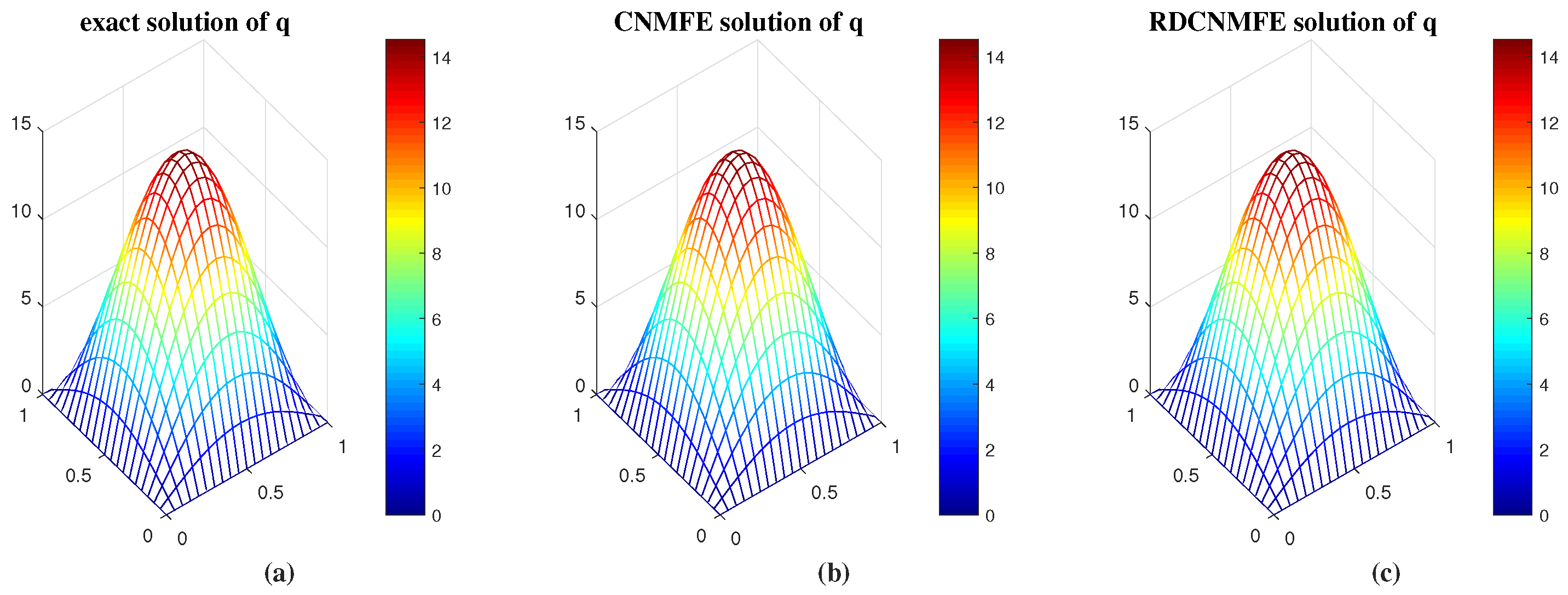
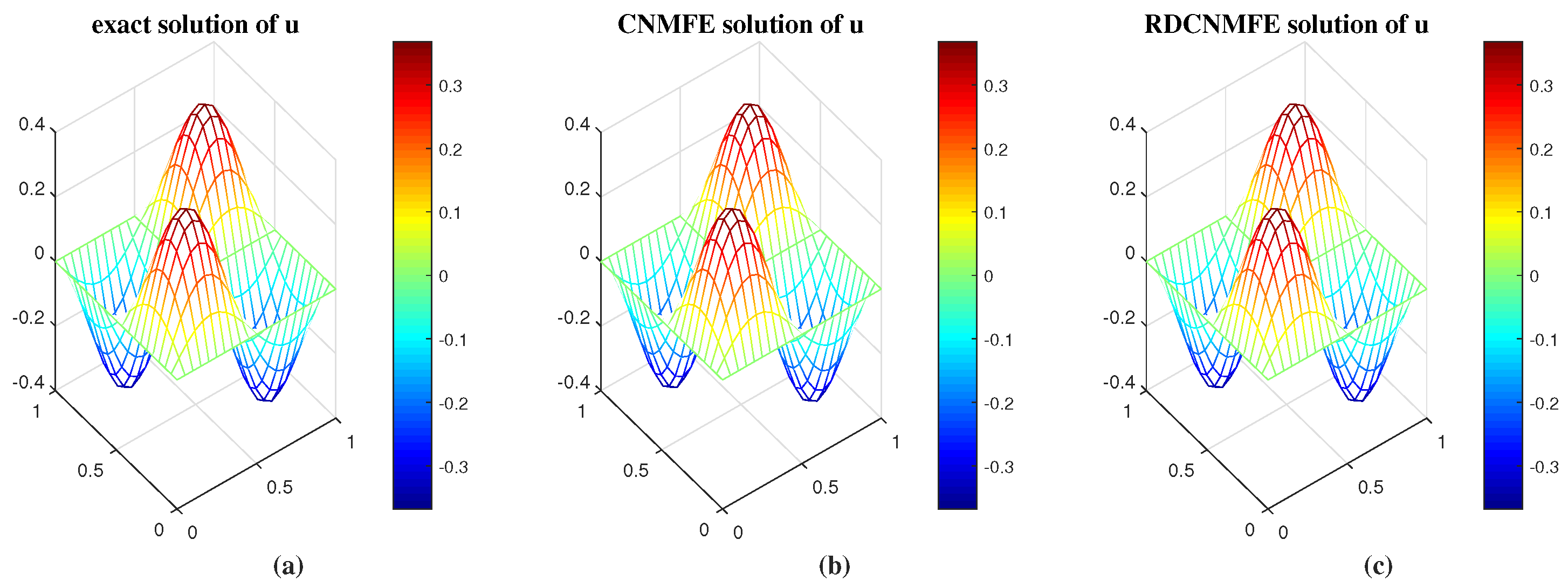
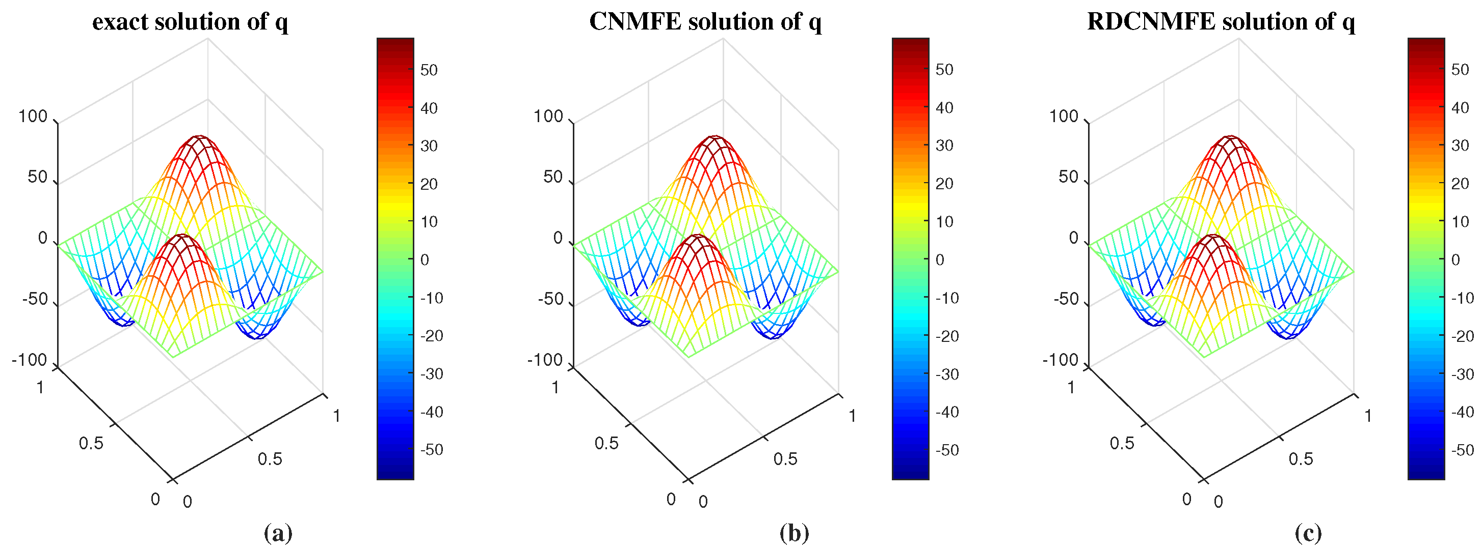
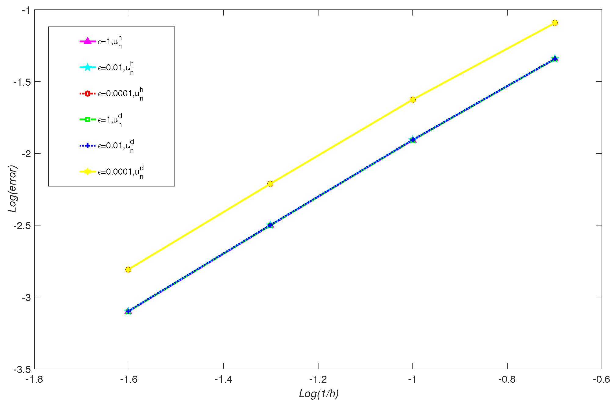
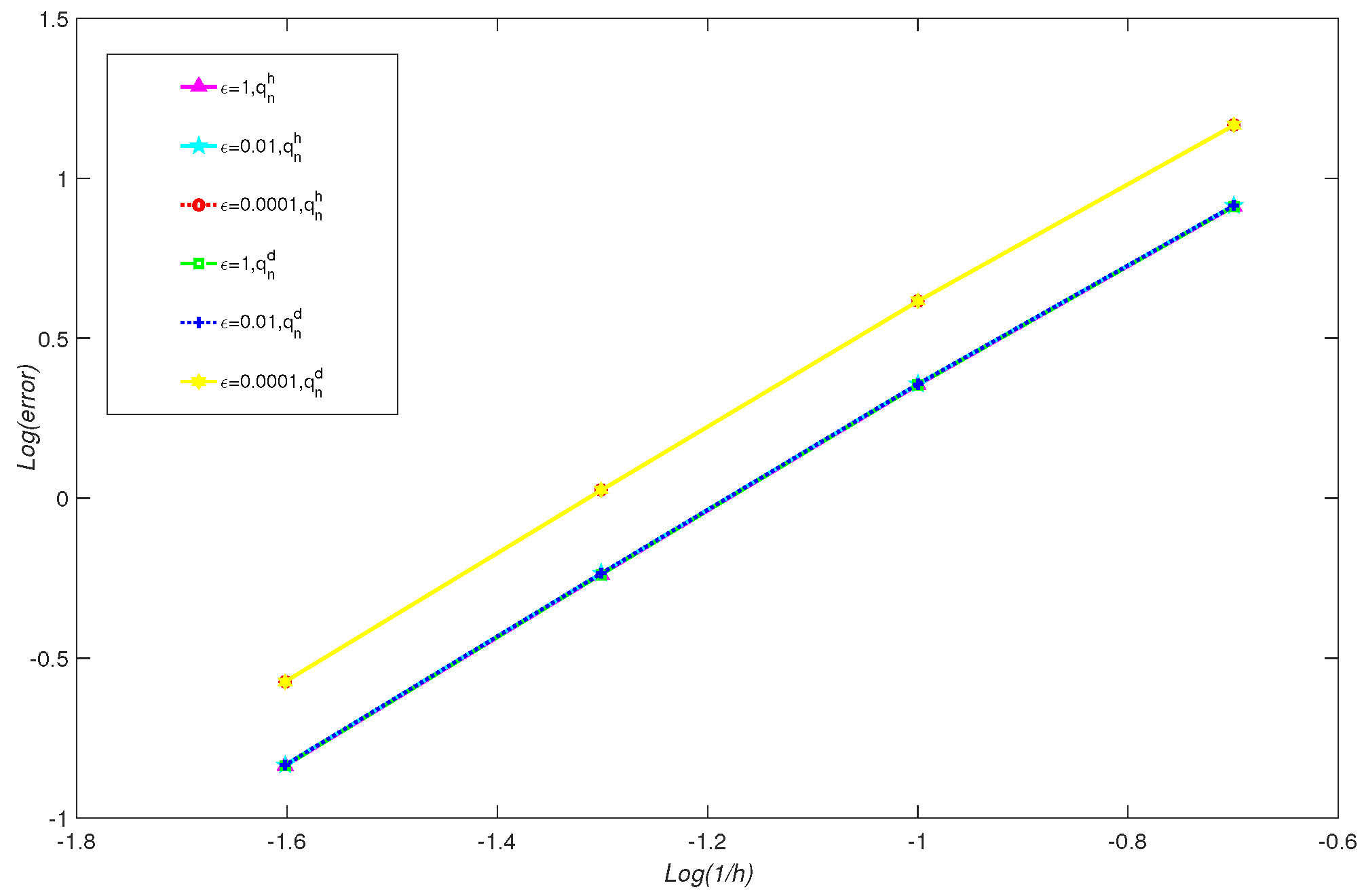
4. The Numerical Experiments for the Fourth-Order Parabolic Equations

For the purpose of assessing the effectiveness of the proposed methods, numerical experiments were conducted. A detailed comparison between the reduced-dimension model and the standard CNMFE model is provided, focusing on the $L^2$ error, convergence orders, and runtime.

4.1. The Fourth-Order Variable Coefficient Parabolic Equation

For analysis, we conducted experiments on the specified fourth-order parabolic equation.

$$\begin{array}{c}\hfill \left\{\begin{array}{cc}{u}_t+\epsilon \nabla ·(b\nabla (\nabla ·(a(t)\nabla u)))-u^3+u=g(x,y,t),\hfill & (x,y,t)\in \Omega \times (0,T],\hfill \\ u(x,y,t)=\Delta u(x,y,t)=0,\hfill & (x,y,t)\in \partial \Omega \times [0,T],\hfill \\ u(x,y,0)=u_0(x,y),\hfill & (x,y)\in \Omega ,\hfill \end{array}\right.\end{array}$$

(108)

Solving Problem 3 yields the standard CNMFE solutions $\{u_h^n,q_h^n\}$. In order to get the RDCNMFE solutions $\{u_d^n,q_d^n\}$, the four steps are as follows.

Step 1:

In order to generate the snapshot matrices ${\mathit{Z}}_1=({\mathit{U}}_h^1,{\mathit{U}}_h^2,\cdots ,{\mathit{U}}_h^{20})$ and ${\mathit{Z}}_2=({\mathit{Q}}_h^1,{\mathit{Q}}_h^2,\cdots ,{\mathit{Q}}_h^{20})$, the initial $\mathcal{K}=20$ CNMFE solution vectors $\{{\mathit{U}}_h^n,{\mathit{Q}}_h^n\}(n=1,2,\cdots ,20)$ are calculated via Problem 3.

Step 2:

Calculate the eigenvalues ${\mu }_{i,j}(i=1,2,j=1,2,\cdots ,20)$ and the corresponding eigenvectors ${\mathit{\varphi }}_{i,j}$ of the matrix ${\mathit{Z}}_i^T{\mathit{Z}}_i$. Sort the eigenvalues in descending order.

Step 3:

Through calculation, it is observed that $\sqrt{{\mu }_{i,7}}⩽h^2+\Delta t^2(i=1,2)$. From the matrix ${\mathit{Z}}_i^T{\mathit{Z}}_i$, the first 6 eigenvectors ${\mathit{\varphi }}_{i,j}(j=1,2,\cdots ,6)$ can be selected. Applying the formula ${\mathit{\phi }}_{i,j}={\mathit{Z}}_i{\mathit{\varphi }}_{i,j}/\sqrt{{\mu }_{i,j}}$, we construct the POD bases ${\mathbf{\Phi }}_i=({\mathit{\phi }}_{i,1},{\mathit{\phi }}_{i,2},\cdots ,{\mathit{\phi }}_{i,6})$.

Step 4:

Inserting the result into Problem 4 and calculating the RDCNMFE solutions.

Example 1.

We explore the model (108) in $\Omega ={[0,1]}^2\subset {\mathbb{R}}^2$ with the analytical solution $u(x,y,t)={\mathrm{e}}^{-t}\sin (\pi x)\sin (\pi y)$. Choosing $a(t)=t^2+1$, $b=1$, the source term is

$$g(x,y,t)={\mathrm{e}}^{-t}(t^2+1)4\epsilon {\pi }^4\sin (\pi x)\sin (\pi y)-{\mathrm{e}}^{-3t}{\sin }^3(\pi x){\sin }^3(\pi y).$$

(109)

Since $q=-\nabla ·(a(t)\nabla u)$, the analytical solution of q is $q(x,y,t)=2{\pi }^2{\mathrm{e}}^{-t}(t^2+1)\sin (\pi x)\sin (\pi y)$.

When $T=1$, with $h=\sqrt{2}/20$ and $\Delta t=1/100$, we get the standard CNMFE solutions and RDCNMFE solutions. They are compared with the exact solutions, as shown in Figure 1 and Figure 2. Obviously, both methods simulate the exact solutions very well.

When $T=1$ and $\Delta t=1/100$, so as to enable an easier comparison, we use both methods to calculate the $L^2$ errors and convergence rates of $\{u,q\}$, as shown in

Table 1. $L^2$ errors and convergence orders between the analytical, CNMFE, and RDCNMFE solutions of u.

		CNMFE Method		RDCNMFE Method
	Grid	$\left|\right|{\mathit{u}}^{\mathit{n}}-{\mathit{u}}_{\mathit{h}}^{\mathit{n}}\left|\right|$	Order	$\left|\right|{\mathit{u}}^{\mathit{n}}-{\mathit{u}}_{\mathit{d}}^{\mathit{n}}\left|\right|$	Order
$\epsilon =1$	$8\times 8$	4.0880 × 10−3		4.0880 × 10−3
	$16\times 16$	1.1926 × 10−3	1.7773	1.1926 × 10−3	1.7773
	$32\times 32$	3.1003 × 10−4	1.9436	3.1003 × 10−4	1.9436
	$64\times 64$	7.7556 × 10−5	1.9991	7.7556 × 10−5	1.9991

and

Table 2. $L^2$ errors and convergence orders between the analytical, CNMFE, and RDCNMFE solutions of q.

		CNMFE Method		RDCNMFE Method
	Grid	$\left|\right|{\mathit{q}}^{\mathit{n}}-{\mathit{q}}_{\mathit{h}}^{\mathit{n}}\left|\right|$	Order	$\left|\right|{\mathit{q}}^{\mathit{n}}-{\mathit{q}}_{\mathit{d}}^{\mathit{n}}\left|\right|$	Order
$\epsilon =1$	$8\times 8$	1.9183 × 10−1		1.9183 × 10−1
	$16\times 16$	5.5050 × 10−2	1.8010	5.5050 × 10−2	1.8010
	$32\times 32$	1.4248 × 10−2	1.9500	1.4248 × 10−2	1.9500
	$64\times 64$	3.5645 × 10−3	1.9990	3.5645 × 10−3	1.9990

.

When $T=1.0,2.0,3.0$, with $h=\sqrt{2}/40$ and $\Delta t=1/100$, we record the $L^2$ error obtained and the CPU runtime required using both methods to further examine the efficacy of the POD-based RDCNMFE method, as shown in

Table 3. Comparison of $L^2$ errors and CPU runtime of CNMFE and RDCNMFE solutions.

Real Time	CNMFE Method			RDCNMFE Method
	$\left|\right|{\mathit{u}}^{\mathit{n}}-{\mathit{u}}_{\mathit{h}}^{\mathit{n}}\left|\right|$	$\left|\right|{\mathit{q}}^{\mathit{n}}-{\mathit{q}}_{\mathit{h}}^{\mathit{n}}\left|\right|$	CPU Runtime	$\left|\right|{\mathit{u}}^{\mathit{n}}-{\mathit{u}}_{\mathit{d}}^{\mathit{n}}\left|\right|$	$\left|\right|{\mathit{q}}^{\mathit{n}}-{\mathit{q}}_{\mathit{d}}^{\mathit{n}}\left|\right|$	CPU Runtime
$T=1.0$	1.9848 × 10−4	9.1218 × 10−3	257.785 s	1.9848 × 10−4	9.1218 × 10−3	61.542 s
$T=2.0$	7.2804 × 10−5	8.7617 × 10−3	518.493 s	7.2804 × 10−5	8.7617 × 10−3	71.464 s
$T=3.0$	2.6836 × 10−5	7.7620 × 10−3	776.562 s	2.6836 × 10−5	7.7620 × 10−3	88.742 s

. The data indicate that both methods obtain the same $L^2$ errors. With each incremental second, the conventional CNMFE method increases by approximately 260 s, whereas the RDCNMFE method only increases by just over 10 s.

Example 2.

We explore the model (108) in $\Omega ={[0,1]}^2\subset {\mathbb{R}}^2$ with the analytical solution $u(x,y,t)={\mathrm{e}}^{-t}\sin (2\pi x)\sin (2\pi y)$. With $a(t)=t^2+1$, $b=1$, the source term is

$$g(x,y,t)={\mathrm{e}}^{-t}(t^2+1)64\epsilon {\pi }^4\sin (2\pi x)\sin (2\pi y)-{\mathrm{e}}^{-3t}{\sin }^3(2\pi x){\sin }^3(2\pi y).$$

(110)

The analytical solution of q is $q(x,y,t)=8{\pi }^2{\mathrm{e}}^{-t}(t^2+1)\sin (2\pi x)\sin (2\pi y)$.

When $T=1$, setting $h=\sqrt{2}/20$ and $\Delta t=1/100$, we employ the CNMFE and RDCNMFE methods to obtain the numerical solutions for Equation (18), which has the noted source term (110). Both solutions to $\{u,q\}$ are compared with the exact solutions. It can be seen clearly from Figure 3 and Figure 4 that both solutions closely approximate the exact solutions.

When $T=1$, setting $\Delta t=1/100$ and $\epsilon =1,0.01,0.0001$, calculating the CNMFE and reduced-dimension solutions of $\{u,q\}$. Then we get the $L^2$ errors and convergence orders of both methods, as shown in

Table 4. $L^2$ errors and convergence orders between the analytical, CNMFE, and RDCNMFE solutions of u.

		CNMFE Method		RDCNMFE Method
	Grid	$\left|\right|{\mathit{u}}^{\mathit{n}}-{\mathit{u}}_{\mathit{h}}^{\mathit{n}}\left|\right|$	Order	$\left|\right|{\mathit{u}}^{\mathit{n}}-{\mathit{u}}_{\mathit{d}}^{\mathit{n}}\left|\right|$	Order
$\epsilon =1$	$5\times 5$	4.5306 × 10−2		4.5306 × 10−2
	$10\times 10$	1.2336 × 10−2	1.8768	1.2336 × 10−2	1.8768
	$20\times 20$	3.1509 × 10−3	1.9691	3.1509 × 10−3	1.9691
	$40\times 40$	7.9192 × 10−4	1.9923	7.9192 × 10−4	1.9923
$\epsilon =0.01$	$5\times 5$	4.5542 × 10−2		4.5542 × 10−2
	$10\times 10$	1.2420 × 10−2	1.8746	1.2420 × 10−2	1.8746
	$20\times 20$	3.1736 × 10−3	1.9684	3.1736 × 10−3	1.9684
	$40\times 40$	7.9778 × 10−4	1.9921	7.9778 × 10−4	1.9921
$\epsilon =0.0001$	$5\times 5$	8.0912 × 10−2		8.0912 × 10−2
	$10\times 10$	2.3697 × 10−2	1.7717	2.3697 × 10−2	1.7717
	$20\times 20$	6.1544 × 10−3	1.9450	6.1544 × 10−3	1.9450
	$40\times 40$	1.5541 × 10−3	1.9856	1.5541 × 10−3	1.9856

and

Table 5. $L^2$ errors and convergence orders between the analytical, CNMFE, and RDCNMFE solutions of q.

		CNMFE Method		RDCNMFE Method
	Grid	$\left|\right|{\mathit{q}}^{\mathit{n}}-{\mathit{q}}_{\mathit{h}}^{\mathit{n}}\left|\right|$	Order	$\left|\right|{\mathit{q}}^{\mathit{n}}-{\mathit{q}}_{\mathit{d}}^{\mathit{n}}\left|\right|$	Order
$\epsilon =1$	$5\times 5$	8.1734 × 100		8.1734 × 100
	$10\times 10$	2.2583 × 100	1.8557	2.2583 × 100	1.8557
	$20\times 20$	5.7873 × 10−1	1.9643	5.7873 × 10−1	1.9643
	$40\times 40$	1.4557 × 10−1	1.9911	1.4557 × 10−1	1.9911
$\epsilon =0.01$	$5\times 5$	8.2168 × 100		8.2168 × 100
	$10\times 10$	2.2721 × 100	1.8546	2.2721 × 100	1.8546
	$20\times 20$	5.8240 × 10−1	1.9639	5.8240 × 10−1	1.9639
	$40\times 40$	1.4651 × 10−1	1.9910	1.4651 × 10−1	1.9910
$\epsilon =0.0001$	$5\times 5$	1.4643 × 101		1.4643 × 101
	$10\times 10$	4.1238 × 100	1.8281	4.1238 × 100	1.8281
	$20\times 20$	1.0595 × 100	1.9605	1.0595 × 100	1.9605
	$40\times 40$	2.6680 × 10−1	1.9896	2.6680 × 10−1	1.9896

. The comparisons of errors for $\{u,q\}$ at $\epsilon =1,0.01,0.0001$ is depicted in Figure 5 and Figure 6. The figures demonstrate that, when $\epsilon$ is set to a very small value, such as $\epsilon =0.0001$, although the solutions obtained by both methods are convergent, their associated errors tend to increase.

The CPU runtime of both methods needs to be compared to further demonstrate the performance of the POD-based reduced-dimension method. When $T=0.5,1.0,1.5,2.0,$$2.5,3.0$, with $h=\sqrt{2}/40$ and $\Delta t=1/100$, we calculated the CNMFE and RDCNMFE solutions. Then, we recorded the CPU runtime required using both methods in

Table 6. Comparison of $L^2$ errors and CPU runtime of CNMFE and RDCNMFE solutions.

Real Time	CNMFE Method			RDCNMFE Method
	$\left|\right|{\mathit{u}}^{\mathit{n}}-{\mathit{u}}_{\mathit{h}}^{\mathit{n}}\left|\right|$	$\left|\right|{\mathit{q}}^{\mathit{n}}-{\mathit{q}}_{\mathit{h}}^{\mathit{n}}\left|\right|$	CPU Runtime	$\left|\right|{\mathit{u}}^{\mathit{n}}-{\mathit{u}}_{\mathit{d}}^{\mathit{n}}\left|\right|$	$\left|\right|{\mathit{q}}^{\mathit{n}}-{\mathit{q}}_{\mathit{d}}^{\mathit{n}}\left|\right|$	CPU Runtime
$T=0.5$	1.3087 × 10−3	1.4793 × 10−1	128.368 s	1.3087 × 10−3	1.4793 × 10−1	56.044 s
$T=1.0$	7.9192 × 10−4	1.4557 × 10−1	254.327 s	7.9192 × 10−4	1.4557 × 10−1	60.044 s
$T=1.5$	4.8003 × 10−4	1.4453 × 10−1	390.405 s	4.8003 × 10−4	1.4453 × 10−1	69.740 s
$T=2.0$	2.9118 × 10−4	1.4011 × 10−1	522.115 s	2.9118 × 10−4	1.4011 × 10−1	76.308 s
$T=2.5$	1.7665 × 10−4	1.3271 × 10−1	650.523 s	1.7665 × 10−4	1.3271 × 10−1	83.345 s
$T=3.0$	1.0718 × 10−4	1.2395 × 10−1	781.210 s	1.0718 × 10−4	1.2395 × 10−1	92.238 s

. As evidenced in Table 6, when the CNMFE method was used, the CPU runtime increased by about 130 s for every additional $0.5$ s. However, when the RDCNMFE method was applied, it took just a few seconds for every added $0.5$ s. The significant reduction in CPU runtime using the reduced-dimension method can be attributed to the difference in degrees of freedom per time step. Specifically, the standard CNMFE method involves $2\times {41}^2$ degrees of freedom, compared to just $2\times 6$ for the RDCNMFE method.

4.2. The Time-Fractional Fourth-Order Parabolic Equation

This part focuses on the numerical simulation of a time-fractional fourth-order parabolic equation.

$$\begin{array}{c}\hfill \left\{\begin{array}{cc}{\displaystyle \frac{{\partial }^{\alpha }u}{\partial t^{\alpha }}+\epsilon \nabla ·(b\nabla (\nabla ·(a(t)\nabla u)))-u^3+u=g(x,y,t),}\hfill & (x,y,t)\in \Omega \times (0,T],\hfill \\ u(x,y,t)=\Delta u(x,y,t)=0,\hfill & (x,y,t)\in \partial \Omega \times [0,T],\hfill \\ u(x,y,0)=u_0(x,y),\hfill & (x,y)\in \Omega ,\hfill \end{array}\right.\end{array}$$

(111)

When the $L1$ discretization scheme is used, the Caputo derivative ${\displaystyle \frac{{\partial }^{\alpha }u}{\partial t^{\alpha }}}$ at $t=t_{n+1}$ can be approximated as:

$${\displaystyle \frac{{\partial }^{\alpha }u(t_{n+1})}{\partial t^{\alpha }}}\approx {\displaystyle \frac{1}{\Gamma (2-\alpha )\Delta t^{\alpha }}}\sum _{k=0}^n{a}_k(u^{n+1-k}-u^{n-k}).$$

(112)

The expression for the coefficient $a_k^{(n)}$ is as follows:

$$a_k={(k+1)}^{1-\alpha }-k^{1-\alpha }.$$

(113)

Example 3.

We explore the model (111) in $\Omega ={[0,1]}^2\subset {\mathbb{R}}^2$ with the analytical solution $u(x,y,t)=t^3\sin (2\pi x)\sin (2\pi y)$. With $a(t)=1$ and $b=1$, the source term is

$$g(x,y,t)=[{\displaystyle \frac{\Gamma (4)}{\Gamma (4-\alpha )}}{t}^{3-\alpha }+t^3(64\epsilon {\pi }^4+1)]\sin (2\pi x)\sin (2\pi y)-t^9{\sin }^3(2\pi x){\sin }^3(2\pi y).$$

(114)

The analytical solution of q is $q(x,y,t)=8{\pi }^2{t}^3\sin (2\pi x)\sin (2\pi y)$.

When $T=1$, numerical solutions to the time-fractional Equation (111) under the specified source term (114) are computed using the CNMFE and RDCNMFE schemes under parameter settings $h=\sqrt{2}/30$ and $\Delta t=1/100$. A comparative analysis between the analytical and numerical solutions of $\{u,q\}$ is presented in Figure 7 and Figure 8. The results demonstrate strong agreement, with both methods yielding approximations that align closely with the analytical solutions.

When $T=1$, with $\Delta t=1/100$, $\epsilon =1,2$, and $\alpha$ ranging from $0.1$ to $0.5$, we numerically solve for the solutions $\{u,q\}$ using both the CNMFE and RDCNMFE methods. The resulting $L^2$ errors and convergence rates are presented in

Table 7. $L^2$ errors and convergence orders between the genuine, CNMFE, and RDCNMFE solutions of u.

			CNMFE Method		RDCNMFE Method
	$\alpha$	Grid	$\left|\right|{\mathit{u}}^{\mathit{n}}-{\mathit{u}}_{\mathit{h}}^{\mathit{n}}\left|\right|$	Order	$\left|\right|{\mathit{u}}^{\mathit{n}}-{\mathit{u}}_{\mathit{d}}^{\mathit{n}}\left|\right|$	Order
$\epsilon =1$	$0.1$	$5\times 5$	1.2310 × 10−1	–	1.2310 × 10−1	–
		$10\times 10$	3.3475 × 10−2	1.8787	3.3475 × 10−2	1.8787
		$20\times 20$	8.5063 × 10−3	1.9765	8.5063 × 10−3	1.9765
		$40\times 40$	2.0939 × 10−3	2.0223	2.0939 × 10−3	2.0223
	$0.2$	$5\times 5$	1.2311 × 10−1	–	1.2311 × 10−1	–
		$10\times 10$	3.3497 × 10−2	1.8779	3.3497 × 10−2	1.8779
		$20\times 20$	8.5312 × 10−3	1.9732	8.5312 × 10−3	1.9732
		$40\times 40$	2.1196 × 10−3	2.0090	2.1196 × 10−3	2.0090
	$0.3$	$5\times 5$	1.2313 × 10−1	–	1.2313 × 10−1	–
		$10\times 10$	3.3497 × 10−2	1.8767	3.3497 × 10−2	1.8767
		$20\times 20$	8.5690 × 10−3	1.9683	8.5690 × 10−3	1.9683
		$40\times 40$	2.1585 × 10−3	1.9891	2.1585 × 10−3	1.9891
	$0.4$	$5\times 5$	1.2316 × 10−1	–	1.2316 × 10−1	–
		$10\times 10$	3.3577 × 10−2	1.8750	3.3577 × 10−2	1.8750
		$20\times 20$	8.6214 × 10−3	1.9615	8.6214 × 10−3	1.9615
		$40\times 40$	2.2125 × 10−3	1.9622	2.2125 × 10−3	1.9622
	$0.5$	$5\times 5$	1.2320 × 10−1	–	1.2320 × 10−1	–
		$10\times 10$	3.3636 × 10−2	1.8729	3.3636 × 10−2	1.8729
		$20\times 20$	8.6877 × 10−3	1.9530	8.6877 × 10−3	1.9530
		$40\times 40$	2.2801 × 10−3	1.9293	2.2801 × 10−3	1.9293
$\epsilon =2$	$0.1$	$5\times 5$	1.2312 × 10−1	–	1.2312 × 10−1	–
		$10\times 10$	3.3503 × 10−2	1.8777	3.3503 × 10−2	1.8777
		$20\times 20$	8.5354 × 10−3	1.9728	8.5354 × 10−3	1.9728
		$40\times 40$	2.1233 × 10−3	2.0072	2.1233 × 10−3	2.0072
	$0.2$	$5\times 5$	1.2313 × 10−1	–	1.2313 × 10−1	–
		$10\times 10$	3.3514 × 10−2	1.8773	3.3514 × 10−2	1.8773
		$20\times 20$	8.5479 × 10−3	1.9711	8.5479 × 10−3	1.9711
		$40\times 40$	2.1361 × 10−3	2.0006	2.1361 × 10−3	2.0006
	$0.3$	$5\times 5$	1.2314 × 10−1	–	1.2314 × 10−1	–
		$10\times 10$	3.3531 × 10−2	1.8767	3.3531 × 10−2	1.8767
		$20\times 20$	8.5668 × 10−3	1.9687	8.5668 × 10−3	1.9687
		$40\times 40$	2.1556 × 10−3	1.9907	2.1556 × 10−3	1.9907
	$0.4$	$5\times 5$	1.2316 × 10−1	–	1.2316 × 10−1	–
		$10\times 10$	3.3554 × 10−2	1.8759	3.3554 × 10−2	1.8759
		$20\times 20$	8.5930 × 10−3	1.9653	8.5930 × 10−3	1.9653
		$40\times 40$	2.1826 × 10−3	1.9771	2.1826 × 10−3	1.9771
	$0.5$	$5\times 5$	1.2317 × 10−1	–	1.2317 × 10−1	–
		$10\times 10$	3.3584 × 10−2	1.8749	3.3584 × 10−2	1.8749
		$20\times 20$	8.6261 × 10−3	1.9510	8.6261 × 10−3	1.9510
		$40\times 40$	2.2168 × 10−3	1.9603	2.2168 × 10−3	1.9603

and

Table 8. $L^2$ errors and convergence orders between the genuine, CNMFE, and RDCNMFE solutions of q.

			CNMFE Method		RDCNMFE Method
	$\alpha$	Grid	$\left|\right|{\mathit{q}}^{\mathit{n}}-{\mathit{q}}_{\mathit{h}}^{\mathit{n}}\left|\right|$	Order	$\left|\right|{\mathit{q}}^{\mathit{n}}-{\mathit{q}}_{\mathit{d}}^{\mathit{n}}\left|\right|$	Order
$\epsilon =1$	$0.1$	$5\times 5$	6.1429 × 100		6.1429 × 100
		$10\times 10$	1.5320 × 100	2.0035	1.5320 × 100	2.0035
		$20\times 20$	3.8003 × 10−1	2.0112	3.8003 × 10−1	2.0112
		$40\times 40$	9.1957 × 10−2	2.0471	9.1957 × 10−2	2.0471
	$0.2$	$5\times 5$	6.1438 × 100		6.1438 × 100
		$10\times 10$	1.5335 × 100	2.0022	1.5335 × 100	2.0022
		$20\times 20$	3.8178 × 10−1	2.0061	3.8178 × 10−1	2.0061
		$40\times 40$	9.3733 × 10−2	2.0261	9.3733 × 10−2	2.0261
	$0.3$	$5\times 5$	6.1454 × 100		6.1454 × 100
		$10\times 10$	1.5359 × 100	2.0004	1.5359 × 100	2.0004
		$20\times 20$	3.8443 × 10−1	1.9983	3.8443 × 10−1	1.9983
		$40\times 40$	9.6452 × 10−2	1.9948	9.6452 × 10−2	1.9948
	$0.4$	$5\times 5$	6.1476 × 100		6.1476 × 100
		$10\times 10$	1.5393 × 100	1.9978	1.5393 × 100	1.9978
		$20\times 20$	3.8813 × 10−1	1.9876	3.8813 × 10−1	1.9876
		$40\times 40$	1.0027 × 10−1	1.9527	1.0027 × 10−1	1.9527
	$0.5$	$5\times 5$	6.1504 × 100		1.4643 × 101
		$10\times 10$	1.5435 × 100	1.9945	1.5435 × 100	1.9945
		$20\times 20$	3.9289 × 10−1	1.9742	3.9289 × 10−1	1.9742
		$40\times 40$	1.0516 × 10−1	1.9012	1.0516 × 10−1	1.9012
$\epsilon =2$	$0.1$	$5\times 5$	6.1447 × 100		6.1447 × 100
		$10\times 10$	1.5340 × 100	2.0021	1.5340 × 100	2.0021
		$20\times 20$	3.8208 × 10−1	2.0054	3.8208 × 10−1	2.0054
		$40\times 40$	9.3990 × 10−2	2.0233	9.3990 × 10−2	2.0233
	$0.2$	$5\times 5$	6.1452 × 100		6.1452 × 100
		$10\times 10$	1.5348 × 100	2.0014	1.5348 × 100	2.0014
		$20\times 20$	3.8295 × 10−1	2.0028	3.8295 × 10−1	2.0028
		$40\times 40$	9.4885 × 10−2	2.0129	9.4885 × 10−2	2.0129
	$0.3$	$5\times 5$	6.1460 × 100		6.1460 × 100
		$10\times 10$	1.5360 × 100	2.0005	1.5360 × 100	2.0005
		$20\times 20$	3.8428 × 10−1	1.9989	3.8428 × 10−1	1.9989
		$40\times 40$	9.6247 × 10−2	1.9973	9.6247 × 10−2	1.9973
	$0.4$	$5\times 5$	6.1470 × 100		6.1470 × 100
		$10\times 10$	1.5376 × 100	1.9992	1.5376 × 100	1.9992
		$20\times 20$	3.8613 × 10−1	1.9936	3.8613 × 10−1	1.9936
		$40\times 40$	9.8147 × 10−2	1.9761	9.8147 × 10−2	1.9761
	$0.5$	$5\times 5$	6.1484 × 100		6.1484 × 100
		$10\times 10$	1.5397 × 100	1.9975	1.5397 × 100	1.9975
		$20\times 20$	3.8846 × 10−1	1.9868	3.8846 × 10−1	1.9868
		$40\times 40$	1.0057 × 10−1	1.9496	1.0057 × 10−1	1.9496

. It is evident that the RDCNMFE method delivers accuracy and convergence performance comparable to those of the traditional CNMFE method.

Furthermore, to demonstrate the computational efficiency of the reduced-dimension method, we recorded the CPU runtime required by both numerical methods. Under fixed parameters $\epsilon =1$, $\alpha =0.2$, $h=\sqrt{2}/40$, and $\Delta t=1/1000$, numerical experiments were conducted for $T=0.5,1.0,1.5,2.0$, and the runtime comparisons between the CNMFE and RDCNMFE methods are summarized in

Table 9. With $\epsilon =1$ and $\alpha =0.2$, a comparison of $L^2$ errors and CPU runtime for CNMFE and RDCNMFE solutions.

Real Time	CNMFE Method			RDCNMFE Method
	$\left|\right|{\mathit{U}}^{\mathit{n}}-{\mathit{U}}_{\mathit{h}}^{\mathit{n}}\left|\right|$	$\left|\right|{\mathit{Q}}^{\mathit{n}}-{\mathit{Q}}_{\mathit{h}}^{\mathit{n}}\left|\right|$	CPU Runtime	$\left|\right|{\mathit{u}}^{\mathit{n}}-{\mathit{u}}_{\mathit{d}}^{\mathit{n}}\left|\right|$	$\left|\right|{\mathit{q}}^{\mathit{n}}-{\mathit{q}}_{\mathit{d}}^{\mathit{n}}\left|\right|$	CPU Runtime
$T=0.5$	2.7163 × 10−4	1.2184 × 10−2	19.797s	2.7163 × 10−4	1.2184 × 10−2	3.605 s
$T=1.0$	2.2003 × 10−3	9.9402 × 10−2	54.301s	2.2003 × 10−3	9.9402 × 10−2	7.574 s
$T=1.5$	7.4754 × 10−3	3.3898 × 10−1	83.899s	7.4754 × 10−3	3.3898 × 10−1	9.907s
$T=2.0$	1.7798 × 10−2	8.0907 × 10−1	141.050 s	1.7798 × 10−2	8.0907 × 10−1	13.984 s

. The results reveal that the RDCNMFE method exhibits a significantly slower growth in computational time as the temporal domain T expands, whereas the CNMFE method suffers from a sharp increase in runtime. Notably, at $T=2.0$, the computational time of the conventional method reaches 10 times that of the RDCNMFE method.

From the numerical results obtained from the above-provided examples, it is evident that the RDCNMFE method based on POD serves as an efficient numerical technique for addressing the fourth-order variable coefficient parabolic equations.

5. Conclusions

In this research, our focus was on reducing the dimension of solution coefficient vectors by employing the CNMFE method combined with the POD technique for the nonlinear variable coefficient fourth-order parabolic equation. Firstly, we developed a CNMFE scheme for the equations. We extensively analyzed the uniqueness, stability, and error estimates of the CNMFE solutions. Afterward, the POD bases were derived from the initial $\mathcal{K}$ CNMFE solution vectors. We constructed a reduced-dimension matrix model and applied conventional FE analysis techniques in order to study the uniqueness, stability, and convergence of the RDCNMFE solutions. Furthermore, we conducted detailed numerical simulations to compare the efficacy of both methods. The RDCNMFE method exhibited a reduced number of degrees of freedom compared to the conventional CNMFE method. This feature significantly reduces the computational load of the RDCNMFE method, thereby decreasing the runtime. Notably, this study has streamlined the calculations by linearizing the nonlinear terms, thereby eliminating repetitive numerical iterations. Thus, the RDCNMFE method emerges as an innovative and efficient numerical approach for addressing complex nonlinear PDEs.

To further validate the generality of the RDCNMFE method, we solved the numerical solutions of time-fractional fourth-order parabolic equations through numerical experiments, demonstrating the effectiveness of the proposed methods. However, the current work lacks a theoretical analysis for time-fractional fourth-order parabolic equations. The experimental results reveal that the existing method fails to maintain applicability when $\epsilon <1$. To address this limitation, future research will extend the POD-based reduced-dimension technique to time-fractional equations, encompassing both theoretical analysis and numerical experiments, and developing an improved framework applicable to cases with $\epsilon <1$. Furthermore, the proposed method exhibits potential for generalization to more complex high-order PDEs, such as spatial-fractional fourth-order PDEs and Schrödinger equations with fourth-order perturbation terms.

References

1. Zhang, T. Finite element analysis for Cahn-Hilliard equation. Math. Numer. Sin. 2006, 28, 281–292. (In Chinese) [Google Scholar]
2. Chai, S.; Wang, Y.; Zhao, W.; Zou, Y. A C0 weak Galerkin method for linear Cahn-Hilliard-Cook equation with random initial condition. Appl. Math. Comput. 2022, 414, 126659. [Google Scholar] [CrossRef]
3. Danumjaya, P.; Pani, A.K. Mixed finite element methods for a fourth order reaction diffusion equation. Numer. Methods Partial Differ. Equ. 2012, 28, 1227–1251. [Google Scholar] [CrossRef]
4. Tian, J.; He, M.; Sun, P. Energy-stable finite element method for a class of nonlinear fourth-order parabolic equations. J. Comput. Appl. Math. 2024, 438, 115576. [Google Scholar] [CrossRef]
5. Zhao, X.; Yang, R.; Qi, R.J.; Sun, H. Energy stability and convergence of variable-step L1 scheme for the time fractional Swift-Hohenberg model. Fract. Calc. Appl. Anal. 2024, 27, 82–101. [Google Scholar] [CrossRef]
6. Barrett, J.W.; Blowey, J.F.; Garcke, H. Finite element approximation of a fourth order nonlinear degenerate parabolic equation. Numer. Math. 1998, 80, 525–556. [Google Scholar] [CrossRef]
7. Du, S.; Cheng, Y.; Li, M. High order spline finite element method for the fourth-order parabolic equations. Appl. Numer. Math. 2023, 184, 496–511. [Google Scholar] [CrossRef]
8. Liu, Y.; Fang, Z.; Li, H.; He, S.; Gao, W. A coupling method based on new MFE and FE for fourth-order parabolic equation. J. Appl. Math. Comput. 2013, 43, 249–269. [Google Scholar] [CrossRef]
9. Liu, Y.; Li, H.; He, S.; Gao, W.; Fang, Z.C. H1-Galerkin mixed element method and numerical simulation for the fourth-order parabolic partial differential equations. Math. Numer. Sin. 2012, 34, 259–274. (In Chinese) [Google Scholar]
10. Shi, D.Y.; Shi, Y.H.; Wang, F.L. Supercloseness and the optimal order error estimates of H1-Galerkin mixed element method for fourth order parabolic equation. Math. Numer. Sin. 2014, 36, 363–380. (In Chinese) [Google Scholar]
11. Li, H.; Guo, Y. The space-time mixed finite element method for fourth order parabolic problems. J. Inn. Mong. Univ. (Natural Sci. Ed.) 2006, 37, 19–22. (In Chinese) [Google Scholar]
12. He, S.; Li, H. The mixed discontinuous space-time finite element method for the fourth order linear parabolic equation with generalized boundary condition. Math. Numer. Sinica. 2009, 31, 167–178. (In Chinese) [Google Scholar]
13. Yin, B.; Liu, Y.; Li, H.; He, S. A two-grid mixed finite element method for a nonlinear fourth-order reaction-diffusion problem with time-fractional derivative. Comput. Math. Appl. 2015, 70, 2474–2492. [Google Scholar]
14. Yin, B.; Liu, Y.; Li, H.; He, S.; Wang, J. TGMFE algorithm combined with some time second-order schemes for nonlinear fourth-order reaction diffusion system. Results. Appl. Math. 2019, 4, 100080. [Google Scholar] [CrossRef]
15. Chai, S.; Zou, Y.; Zhou, C.; Zhao, W. Weak Galerkin finite element methods for a fourth order parabolic equation. Numer. Methods Partial. Differ. Equ. 2019, 35, 1745–1755. [Google Scholar] [CrossRef]
16. Zhao, X.; Liu, F.; Liu, B. Finite difference discretization of a fourth-order parabolic equation describing crystal surface growth. Appl. Anal. 2015, 94, 1–15. [Google Scholar] [CrossRef]
17. Mohanty, R.K.; Kaur, D.; Singh, S. A class of two- and three-level implicit methods of order two in time and four in space based on half-step discretization for two-dimensional fourth order quasi-linear parabolic equations. Appl. Math. Comput. 2019, 352, 68–87. [Google Scholar] [CrossRef]
18. Kaur, D.; Mohanty, R.K. Highly accurate compact difference scheme for fourth order parabolic equation with Dirichlet and Neumann boundary conditions: Application to good Boussinesq equation. Appl. Math. Comput. 2020, 378, 125202. [Google Scholar] [CrossRef]
19. Gao, G.; Huang, Y.; Sun, Z. Pointwise error estimate of the compact difference methods for the fourth-order parabolic equations with the third Neumann boundary conditions. Math. Meth. Appl. Sci. 2023, 47, 634–659. [Google Scholar] [CrossRef]
20. Kaur, D.; Mohanty, R.K. High-order half-step compact numerical approximation for fourth-order parabolic PDEs. Numer. Algorithms 2024, 95, 1127–1153. [Google Scholar] [CrossRef]
21. Sharma, S.; Sharma, N. A fast computational technique to solve fourth-order parabolic equations: Application to good Boussinesq, Euler-Bernoulli and Benjamin-Ono equations. Int. J. Comput. Math. 2024, 101, 194–216. [Google Scholar] [CrossRef]
22. Ishige, K.; Miyake, N.; Okabe, S. Blowup for a Fourth-Order Parabolic Equation with Gradient Nonlinearity. SIAM J. Math. Anal. 2020, 52, 927–953. [Google Scholar] [CrossRef]
23. Ding, H.; Zhou, J. Infinite Time Blow-Up of Solutions to a Fourth-Order Nonlinear Parabolic Equation with Logarithmic Nonlinearity Modeling Epitaxial Growth. Mediterr. J. Math. 2021, 18, 1–19. [Google Scholar] [CrossRef]
24. Shao, X.; Tang, G. Blow-up phenomena for a class of fourth order parabolic equation. J. Math. Anal. Appl. 2021, 505, 125445. [Google Scholar] [CrossRef]
25. Zhao, J.; Guo, B.; Wang, J. Global existence and blow-up of weak solutions for a fourth-order parabolic equation with gradient nonlinearity. Z. Angew. Math. Phys. 2024, 75, 1–12. [Google Scholar] [CrossRef]
26. Luo, Z.D. Finite Element and Reduced Dimension Methods for Partial Differential Equations; Springer: Singapore; Beijing, China, 2024. [Google Scholar]
27. Luo, Z.D.; Chen, G. Proper Orthogonal Decomposition Methods for Partial Differential Equations; Academic Press of Elsevier: San Diego, CA, USA, 2018. [Google Scholar]
28. Shao, W.; Chen, C. A fourth order Runge-Kutta type of exponential time differencing and triangular spectral element method for two dimensional nonlinear Maxwell’s equations. Appl. Numer. Math. 2025, 207, 348–369. [Google Scholar] [CrossRef]
29. Zeiser, A. Sparse grid time-discontinuous Galerkin method with streamline diffusion for transport equations. Partial. Differ. Equ. Appl. 2023, 4, 38. [Google Scholar] [CrossRef]
30. Jiang, S.; Cheng, Y.; Cheng, Y.; Huang, Y. Generalized multiscale finite element method and balanced truncation for parameter-dependent parabolic problems. Mathematics 2023, 11, 4695. [Google Scholar] [CrossRef]
31. Xu, B.; Zhang, X.; Ji, D. A Reduced High-Order Compact Finite Difference Scheme Based on POD Technique for the Two Dimensional Extended Fisher-Kolmogorov Equation. IAENG Int. J. Appl. Math. 2020, 50, 474–483. [Google Scholar]
32. Li, Q.; Chen, H.; Wang, H. A proper orthogonal decomposition-compact difference algorithm for plate vibration models. Numer. Algorithms 2023, 94, 1489–1518. [Google Scholar] [CrossRef]
33. Zhao, W.; Piao, G.R. A reduced Galerkin finite element formulation based on proper orthogonal decomposition for the generalized KDV-RLW-Rosenau equation. J. Inequal. Appl. 2023, 2023, 104. [Google Scholar] [CrossRef]
34. Garcia-Archilla, B.; John, V.; Novo, J. Second order error bounds for POD-ROM methods based on first order divided differences. Appl. Math. Letters 2023, 146, 108836. [Google Scholar] [CrossRef]
35. Janes, A.; Singler, R.J. A new proper orthogonal decomposition method with second difference quotients for the wave equation. J. Comput. Appl. Math. 2025, 457, 116279. [Google Scholar] [CrossRef]
36. He, S.; Li, H.; Liu, Y. A POD based extrapolation DG time stepping space-time FE method for parabolic problems. J. Math. Anal. Appl. 2024, 539, 128501. [Google Scholar] [CrossRef]
37. Lu, J.; Zhang, L.; Guo, X.; Qi, Q. A POD based reduced-order local RBF collocation approach for time-dependent nonlocal diffusion problems. Appl. Math. Letters 2025, 160, 109328. [Google Scholar] [CrossRef]
38. Luo, Z.D.; Li, L.; Sun, P. A reduced-order MFE formulation based on POD method for parabolic equations. Acta. Math. Sci. 2013, 33B, 1471–1484. [Google Scholar] [CrossRef]
39. Liu, Q.; Teng, F.; Luo, Z.D. A reduced-order extrapolation algorithm based on CNLSMFE formulation and POD technique for two-dimensional Sobolev equations. Appl. Math. Ser. B. 2014, 29, 171–182. [Google Scholar] [CrossRef]
40. Luo, Z.D.; Zhou, Y.J.; Yang, X.Z. A reduced finite element formulation based on proper orthogonal decomposition for Burgers equation. Appl. Numer. Math. 2009, 59, 1933–1946. [Google Scholar] [CrossRef]
41. Song, J.; Rui, H. A reduced-order characteristic finite element method based on POD for optimal control problem governed by convection-diffusion equation. Comput. Meth. Appl. M 2022, 391, 114538. [Google Scholar] [CrossRef]
42. Song, J.; Rui, H. Reduced-order finite element approximation based on POD for the parabolic optimal control problem. Numer. Algorithms 2024, 95, 1189–1211. [Google Scholar] [CrossRef]
43. Luo, Z.D. A POD-Based Reduced-Order Stabilized Crank-Nicolson MFE Formulation for the Non-Stationary Parabolized Navier-Stokes Equations. Math. Model. Anal. 2015, 20, 346–368. [Google Scholar] [CrossRef]
44. Luo, Z.D. A POD-based reduced-order TSCFE extrapolation iterative format for two-dimensional heat equations. Bound. Value. Probl. 2015, 2015, 1–15. [Google Scholar] [CrossRef]
45. Luo, Z.D. The reduced-order extrapolating method about the Crank-Nicolson finite element solution coefficient vectors for parabolic type equation. Mathematics. 2020, 8, 1261. [Google Scholar] [CrossRef]
46. Zeng, Y.; Luo, Z.D. The reduced-dimension technique for the unknown solution coefficient vectors in the Crank-Nicolson finite element method for the Sobolev equation. J. Math. Anal. Appl. 2022, 513, 126207. [Google Scholar] [CrossRef]
47. Teng, F.; Luo, Z.D. A reduced-order extrapolation technique for solution coefficient vectors in the mixed finite element method for the 2D nonlinear Rosenau equation. J. Math. Anal. Appl. 2020, 485, 123761. [Google Scholar] [CrossRef]
48. Luo, Z.D. The dimensionality reduction of Crank-Nicolson mixed finite element solution coefficient vectors for the unsteady Stokes equation. Mathematics 2022, 10, 2273. [Google Scholar] [CrossRef]
49. Li, Y.; Teng, F.; Zeng, Y.; Luo, Z. Two-grid dimension reduction method of Crank-Nicolson mixed finite element solution coefficient vectors for the fourth-order extended Fisher-Kolmogorov equation. J. Math. Anal. Appl. 2024, 536, 128168. [Google Scholar] [CrossRef]
50. Chang, X.; Li, H. The reduced-dimension method for Crank-Nicolson mixed finite element solution coefficient vectors of the extended Fisher-Kolmogorov equation. Axioms 2024, 13, 710. [Google Scholar] [CrossRef]
51. Zeng, Y.; Li, Y.; Zeng, Y.; Cai, Y.; Luo, Z. The dimension reduction method of two-grid Crank-Nicolson mixed finite element solution coefficient vectors for nonlinear fourth-order reaction diffusion equation with temporal fractional derivative. Commun. Nonlinear. Sci. 2024, 133, 107962. [Google Scholar] [CrossRef]
52. Adams, R.A. Sobolev Spaces; Academic Press: New York, USA, 1975. [Google Scholar]
53. Luo, Z.D. The Founfations and Applications of Mixed Finite Element Methods; Chinese Science Press: Beijing, China, 2006. (In Chinese) [Google Scholar]
54. Wang, J.F.; Li, H.; He, S.; Gao, W.; Liu, Y. A new linearized Crank-Nicolson mixed element scheme for the extended Fisher-Kolmogorov equation. Sci. World J. 2013, 2013, 756281. [Google Scholar] [CrossRef]
Figure 1. (a) The exact solution u n . (b) The CNMFE solution u h n . (c) The RDCNMFE solution u d n .
Fractalfract 09 00137 g001
Figure 2. (a) The exact solution q n . (b) The CNMFE solution q h n . (c) The RDCNMFE solution q d n .
Fractalfract 09 00137 g002
Figure 3. (a) The exact solution u n . (b) The CNMFE solution u h n . (c) The RDCNMFE solution u d n .
Fractalfract 09 00137 g003
Figure 4. (a) The exact solution q n . (b) The CNMFE solution q h n . (c) The RDCNMFE solution q d n .
Fractalfract 09 00137 g004
Figure 5. Comparison of error results of u when ε = 1 , 0.01 , 0.0001 .
Fractalfract 09 00137 g005
Figure 6. Comparison of error results of q when ε = 1 , 0.01 , 0.0001 .
Fractalfract 09 00137 g006
Figure 7. (a) The exact solution u n . (b) The CNMFE solution u h n . (c) The RDCNMFE solution u d n .
Fractalfract 09 00137 g007
Figure 8. (a) The exact solution q n . (b) The CNMFE solution q h n . (c) The RDCNMFE solution q d n .
Fractalfract 09 00137 g008