Parameter Estimation of Fractional Uncertain Differential Equations

Abstract

In this paper, we focus on the parameter estimations and some related issues of a class of fractional uncertain differential equations. We obtain the parameter estimations of the considered equations by using rectangular and trapezoidal algorithms for numerical approximation of optimal problems. Subsequently, by taking the trapezoidal method as an example, the predicted variable–corrected variable method is used to solve fractional-order uncertain differential equations, and numerical solutions were demonstrated by using different $\alpha$-paths. Finally, by using the trapezoidal algorithm, we predicted the closing prices of Tencent Holdings for the entire year of 2023 and compared them with actual historical values, showcasing the applicability and effectiveness of this method in practical applications.

1. Introduction

Randomness and uncertainty are ubiquitous in our daily lives, such as guessing the size of points before rolling dice, predicting future weather conditions, and predicting stocks of a certain company. These phenomena demonstrate the inherent unpredictability and variability in various aspects of life. Recognizing this, researchers have long attempted to understand and quantify uncertainty systematically. Probability theory, which was founded on Kolmogorov’s axiomatic framework, has become a fundamental mathematical tool for analyzing random phenomena. It views randomness as an essential characteristic of objective uncertainty. In contrast, Zadeh [1] introduced fuzzy sets in 1965, which are characterized by membership functions, and later [2] proposed the theory of possibility to quantify fuzzy events. Nevertheless, it has been observed that many uncertain phenomena in reality do not neatly fit into the categories of randomness or fuzziness. To address this gap, Liu [3] developed uncertainty theory, which is designed to handle situations involving subjective uncertainty. While probability theory is centered around the frequency of occurrences, uncertainty theory focuses on the degree of belief associated with uncertain events. A well-known benchmark problem [3] provides a clear framework for distinguishing between the appropriate contexts for applying probability theory and uncertainty theory.

Uncertain differential equations, a type of differential equation driven by a canonical process $C_t$, were first introduced by Liu [3] in 2007 as part of uncertain calculus theory. Since their introduction, these equations have become a focal point of research due to their wide-ranging applications in areas such as finance, biology, economics, and engineering. For example, the existence and uniqueness of solutions were investigated in [4,5,6,7,8]; stability properties were examined in [9,10,11,12]; uncertain optimal control problems were analyzed by [7,13,14]; and numerical approximation methods were explored by [12,15,16,17,18].

On the other hand, the fractional derivative describes memory and genetic effects and has received a lot of attention due to its wide range of applications in biology, chemistry, economics, and engineering. In contrast to the classical derivative, the fractional derivative of a constant is not zero. Due to theoretical development and practical application, there has been increasing interest in various fractional differential equations, as seen in [19,20,21] and in recent works on multi-term fractional impulsive systems [22,23,24].

The estimation of unknown parameters is a crucial issue in uncertain differential equations, particularly when only discrete observations are available. Initially, Yao and Liu [25] introduced the method of moments based on the Euler method. Later, Liu and Jia [26] extended this method to parameter estimation for uncertain delay differential equations. Since then, the application of the Euler method in parameter estimation has expanded, with several new methods proposed and extensively studied. For instance, significant advances have been made, such as generalized moment estimation [27] and least squares estimation [28]. However, the Euler method remains the simplest difference scheme for approximating uncertain differential equations. To enhance accuracy, Tang [11] derived the Milstein scheme for uncertain differential equations, inspired by the Milstein method [29] for stochastic differential equations. This new method has also been successfully applied to parameter estimation. Additionally, Yang et al. [30] introduced the minimum cover estimation method for estimating unknown parameters in uncertain differential equations. Furthermore, refs. [7,25,31] have contributed a series of related studies on parameter estimation, along with further developments in stability and numerical methods [12,32,33].

Wu [34] proposed a new method in 2022 that combines the Adams numerical method with its optimization algorithm to estimate unknown parameters by constructing a minimization optimization problem. This method provides more parameter degrees of freedom and can better fit actual data and improve prediction accuracy compared to traditional UDE methods. To expand its research on parameter estimation accuracy, we introduce rectangular and trapezoidal algorithms to numerically approximate the optimization problem, and use prediction–correction methods to solve FUDEs. This method not only enhances parameter estimation accuracy but also provides numerical solutions for various $\alpha$-path values, highlighting its efficacy, enhancing the application effect of uncertainty analysis, and further developing parameter estimation methods.

In this article, we will continue to investigate parameter estimation and related issues for a class of fractional uncertain differential equations.

The contributions of this paper can be summarized as follows:

(1)

A novel approach for estimating parameters of FUDEs is introduced. In particular, the rectangular and trapezoidal methods are utilized for the numerical approximation of optimization problems.

(2)

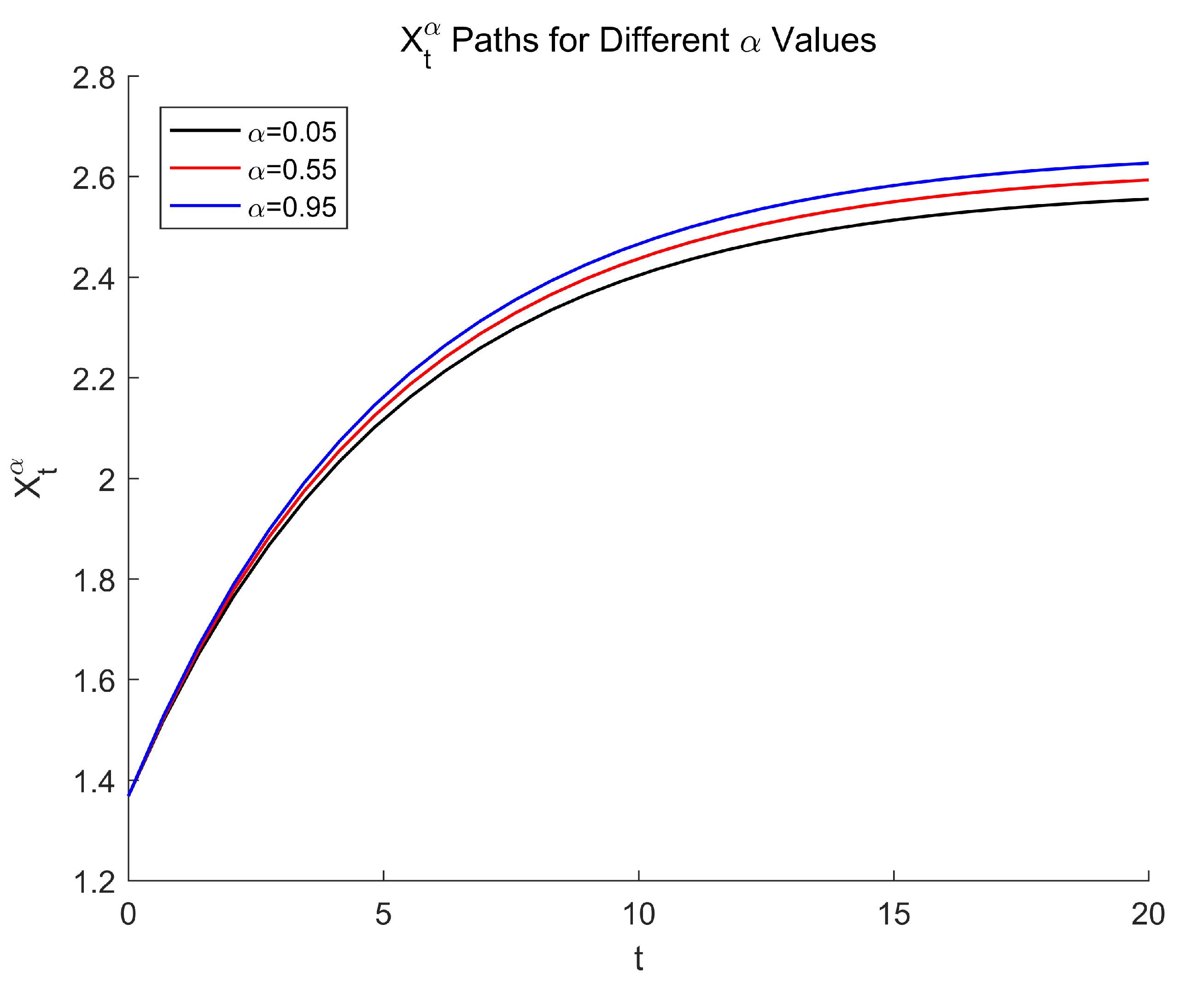
The prediction–correction technique is employed to solve fractional-order uncertain differential equations, with expected values being derived through the $\alpha$-path method. Numerical simulations are carried out along various $\alpha$-paths, yielding corresponding numerical solutions.

(3)

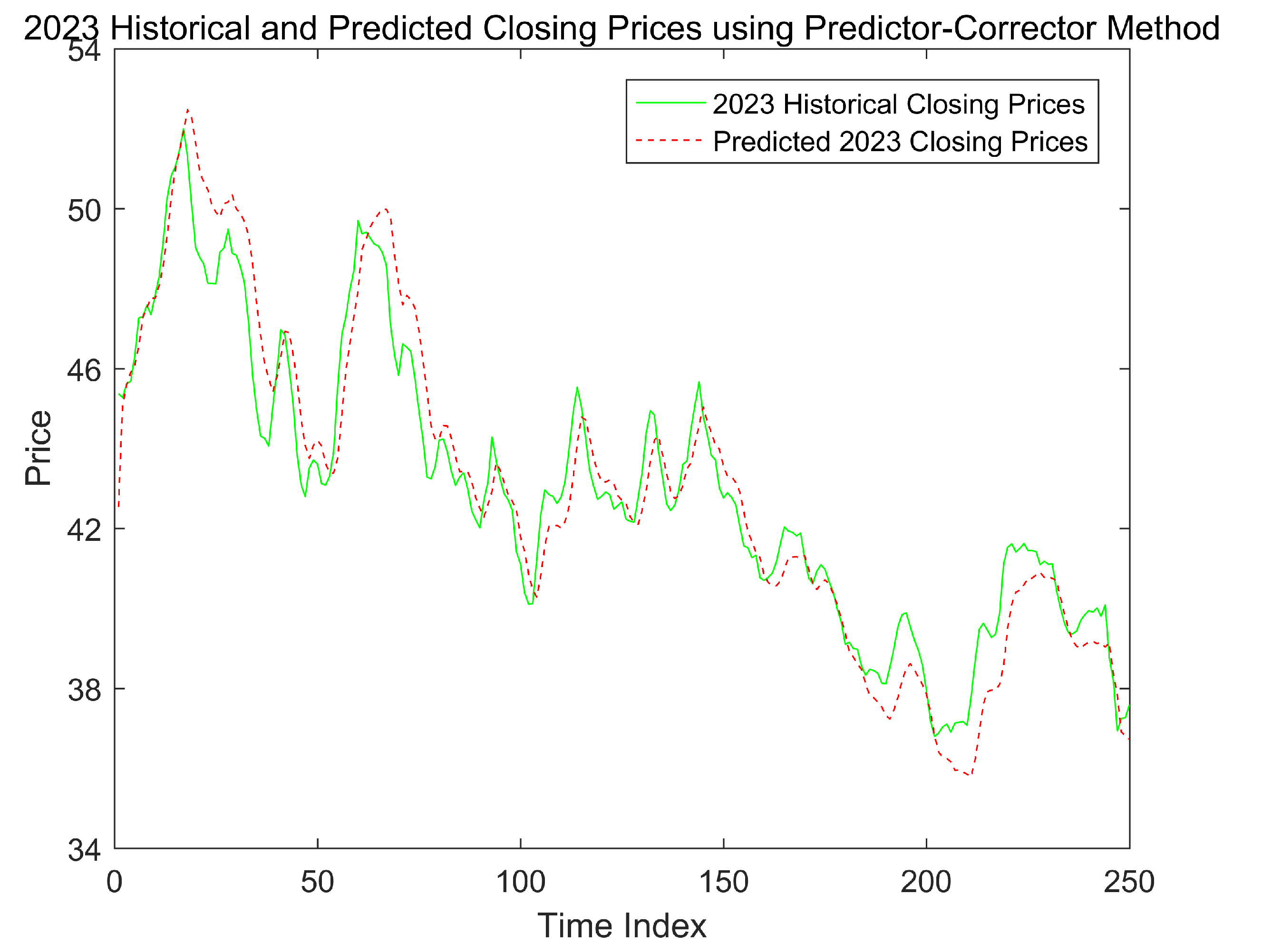
Finally, the proposed method is applied to practical models for prediction, demonstrating its applicability and robustness.

The article is organized as follows: In Section 2, we reviewed some useful concepts about uncertain variables and uncertain differential equations. In Section 3, we introduced a new method for estimating the unknown parameters of a FUDE using the rectangular method and the trapezoidal method. In Section 4, taking the trapezoidal method as an example, we solved the FUDE under initial conditions and provided numerical solutions for different $\alpha$-paths. In Section 5, we applied this method to the stock of Tencent Holdings Limited and predicted its closing price for the entire year of 2023. In Section 6, a brief overview of the entire text was provided.

2. Preliminaries

Let us first revisit some basics of the uncertainty theory.

Definition 1

(See [3]). Let $\mathcal{L}$ be a σ-algebra on a nonempty set Γ. A set function $\mathcal{M}:\mathcal{L}\to [0,1]$ is called an uncertain measure if it satisfies the following four axioms:

• (A1) Normality axiom. $\mathcal{M}\{\Gamma \}=1$ for the universal set Γ.
• (A2) Duality axiom. $\mathcal{M}\{\Lambda \}+\mathcal{M}\left\{{\Lambda }^c\right\}=1$ for any event Λ.
• (A3) Subadditivity axiom. For every countable sequence of events ${\Lambda }_1,{\Lambda }_2,\dots$, we have

  $$\mathcal{M}\left\{\bigcup _{i=1}^{\infty }{\Lambda }_i\right\}\le \sum _{i=1}^{\infty }\mathcal{M}\left\{{\Lambda }_i\right\}.$$
• (A4) Product axiom. Let $({\Gamma }_k,{\mathcal{L}}_k,{\mathcal{M}}_k)$ be uncertain spaces for $k=1,2,\dots$. Then, the product uncertain measure $\mathcal{M}$ satisfies

  $$\mathcal{M}{\{}_{k=1}^{\infty }{\Lambda }_k\}=\underset{k=1}{\overset{\infty }{\bigwedge }}{\mathcal{M}}_k\left\{{\Lambda }_k\right\},$$
  where ${\Lambda }_k$ is an arbitrarily chosen event from ${\mathcal{L}}_k$ for $k=1,2,\dots$, respectively.

Definition 2

(See [3]). Let ξ be an uncertain variable on an uncertain space $(\Gamma ,\mathcal{L},\mathcal{M})$. Then, its expected value $E\left[\xi \right]$ is

$$E\left[\xi \right]={\int }_0^{+\infty }\mathcal{M}\{\xi \ge x\}dx-{\int }_{-\infty }^0\mathcal{M}\{\xi <x\}dx,$$

provided that at least one of the two integrals ${\int }_0^{+\infty }\mathcal{M}\{\xi \ge x\}dx$ and ${\int }_{-\infty }^0\mathcal{M}\{\xi <x\}dx$ exists, and its variance $V\left[\xi \right]$ is

$$V\left[\xi \right]=E\left[{(\xi -E\left[\xi \right])}^2\right].$$

Definition 3

(See [3]). An uncertain process $C_t$ is called a Liu process if

(i) 

$C_0=0$, and almost all simple paths are Lipschitz continuous;

(ii) 

$C_t$ has stationary and independent increments;

(iii) 

The increment $C_{s+t}-C_s$ has a normal uncertain distribution

$${\Phi }_t(x)={\left(1+exp\left(-{\displaystyle \frac{\pi x}{\sqrt{3}t}}\right)\right)}^{-1},x\in \mathbb{R}.$$

The fractional calculus is defined as follows.

Definition 4

(See [35,36]). Let $x(t)$ be a continuous function and $x(t)\in L^1[a,T]$. The Riemann–Liouville integral for $\nu >0$ is defined by

$$a{I}_t^{\nu }x(t)={\displaystyle \frac{1}{\Gamma (\nu )}}{\int }_a^t{\displaystyle \frac{x(s)}{{(t-s)}^{1-\nu }}}ds,t>a.$$

For $\nu =1$, the fractional integral becomes the standard integral $a{I}_t^{1}x(t)={\int }_a^{t}x(s)ds$, $t>a$.

If $\nu \ne 1,2,3,\dots$, the fractional integral holds memory effects, and $1/{(t-s)}^{1-\nu }$ is called a weight or memory function.

Definition 5

(See [35,36]). Let $x(t)\in AC[a,T]$. The Caputo derivative for $0<\nu <1$ is defined by

$${}^{C}D_a^v{X}_t={\displaystyle \frac{1}{\Gamma (1-\nu )}}{\int }_a^t{\displaystyle \frac{x^{\prime }(s)}{{(t-s)}^{\nu }}}ds,t>a,$$

for $\nu =1$, ${}^{C}D_a^{v}x(t)=dx/dt$.

Suppose that $f:[a,+\infty )\times {\mathbb{R}}^n$ and $g:[a,+\infty )\times {\mathbb{R}}^n$ are two functions. The FUDE of the Caputo type can be presented as

$${}^{C}D_a^v{X}_a=f(t,X_t;\mu )+g(t,X_t;\sigma ){\displaystyle \frac{d{C}_t}{dt}},0<\nu \le 1,X_{t=a}=X_a,$$

(1)

where μ and σ are the parameters in drift term $f(t,X_t;\mu )$ and diffusion term $g(t,X_t;\sigma )$, respectively.

In this paper, we consider fractional-order uncertain differential Equation (1), and to ensure the validity of its solution, we introduce two assumptions of Lemma 1.

Lemma 1

([8]). The FUDE (1) has a unique solution $X_t$ on $[a,+\infty )$ if for all $x,y\in {\mathbb{R}}^n$ and $t\in [a,+\infty )$, the coefficient functions $f(t,x)$ and $g(t,x)$ satisfy

(H1) 

Lipschitz condition $\parallel f(t,x)-f(t,y)\parallel +\parallel g(t,x)-g(t,y)\parallel \le L\parallel x-y\parallel$,

(H2) 

linear growth condition $\parallel f(t,x)-f(t,y)\parallel +\parallel g(t,x)-g(t,y)\parallel \le L\parallel x-y\parallel$,

where L is a positive constant, and $\parallel ·\parallel$ is a norm. Furthermore, $X_t$ is sample continuous.

3. Parameter Estimation

In this section, we perform parameter estimation on fractional-order uncertain differential equations, using the fractional step method and fractional-order rectangle method for numerical approximation. Optimization algorithms are also included, as shown below.

3.1. Discretization Model of the Fractional-Order Rectangular Method

Let us consider the fractional differential equation

$${}_a{}^{C}D_t^{v}x(t)=F(t,x),0<\nu \le 1,x(a)=x_a,$$

(2)

where $\varphi (t)$ solves Equation (2) if and only if $\varphi (t)$ is a solution of the fractional integral equation

$$x(t)=x_a+a{I}_t^{\nu }F(t,x),x(a)=x_a.$$

Using a uniform time division $[a,b]$: $a=t_0<t_1<\dots <t_n<t_{n+1}=b$, we use the approximate formula for the fractional rectangular step method

$$x_{n+1}=x_0+{\displaystyle \frac{1}{\Gamma (\nu +1)}}\sum _{i=0}^n{c}_{i}F(t_i,x_i),$$

(3)

where

$$c_i=\left\{\begin{array}{cc}{(t_i-t_0)}^{\nu },\hfill & i=0,\hfill \\ {(t_{i+1}-t_i)}^{\nu },\hfill & i=1,\dots ,n-1,\hfill \\ {(t_{n+1}-t_n)}^{\nu },\hfill & i=n.\hfill \end{array}\right.$$

The FUDE (1) has a solution given by

$$\begin{array}{cc}\hfill X_{t_{n+1}}=X_{t_0}& +{\displaystyle \frac{1}{\Gamma (\nu )}}{\int }_{t_0}^{t_{n+1}}{(t_{n+1}-s)}^{\nu -1}f(t_i,X_s;\mu )ds\hfill \\ \hfill & +{\displaystyle \frac{1}{\Gamma (\nu )}}{\int }_{t_0}^{t_{n+1}}{(t_{n+1}-s)}^{\nu -1}g(t_i,X_s;\sigma )d{C}_s.\hfill \end{array}$$

(4)

First, according to the definition of the Liu integral from [3], the numerical discretization is given by

$${\displaystyle \frac{1}{\Gamma (\nu )}}{\int }_{t_0}^{t_{n+1}}{(t_{n+1}-s)}^{\nu -1}g(t_i,X_s;\sigma )d{C}_s\approx {\displaystyle \frac{1}{\Gamma (\nu )}}\sum _{i=0}^n{(t_{n+1}-t_i)}^{\nu -1}g(t_i,X_{t_i};\sigma )(C_{t_{i+1}}-C_{t_i}).$$

Then, using the fractional-order trapezoidal method (3), the numerical approximation of Equation (4) can be written as

$$X_{t_{n+1}}=X_{t_0}+{\displaystyle \frac{1}{\Gamma (\nu +1)}}\sum _{i=0}^n{c}_{i}f(t_i,X_{t_i};\mu )+{\displaystyle \frac{1}{\Gamma (\nu )}}\sum _{i=0}^n{(t_{n+1}-t_i)}^{\nu -1}g(t_i,X_{t_i};\sigma )(C_{t_{i+1}}-C_{t_i}),$$

obtaining after transfer

$$\begin{array}{cc}\hfill & {\displaystyle \frac{1}{\Gamma (\nu )}}\sum _{i=0}^n{(t_{n+1}-t_i)}^{\nu -1}g(t_i,X_{t_i};\sigma )(C_{t_{i+1}}-C_{t_i})\hfill \\ \hfill =& X_{t_{n+1}}-X_{t_0}-{\displaystyle \frac{1}{\Gamma (\nu +1)}}\sum _{i=0}^n{c}_{i}f(t_i,X_{t_i};\mu ).\hfill \end{array}$$

(5)

The term on the left-hand side of Equation (5) is considered as “noise” and should be minimized. Using the observed data $(t_i,X_{t_i})$ for $i=0,1,\dots ,N,N+1$, the parameter estimation for $\mu$ and $\nu$ involves solving the following minimization problem

$$\underset{\mu ,\nu }{min}\sum _{n=0}^N{\left(X_{t_{n+1}}-X_{t_0}-{\displaystyle \frac{1}{\Gamma (\nu +1)}}\sum _{i=0}^n{c}_{i}f(t_i,X_{t_i};\mu )\right)}^2.$$

(6)

Suppose $({\mu }^{\ast },{\nu }^{\ast })$ is the optimal solution of the minimum optimization problem (6). Next, taking the expected value to Equation (5), we have

$$\begin{array}{cc}\hfill & \mathbb{E}\left[\sum _{n=0}^N{\left({\displaystyle \frac{1}{\Gamma ({\nu }^{\ast })}}\sum _{i=0}^n({(t_{n+1}-t_i)}^{{\nu }^{\ast }-1}g(t_i,X_{t_i};\sigma )(C_{t_{i+1}}-C_{t_i})\right)}^2\right]\hfill \\ \hfill & =\sum _{n=0}^N{\left(X_{t_{n+1}}-X_{t_0}-{\displaystyle \frac{1}{\Gamma ({\nu }^{\ast }+1)}}\sum _{i=0}^n{c}_{i}f(t_i,X_{t_i};{\mu }^{\ast })\right)}^2.\hfill \end{array}$$

(7)

Given that $C_{t_i}$ is a stationary process with independent increments, each difference $C_{t_{i+1}}-C_{t_i}$ represents a normal uncertain variable characterized by an expected value of 0 and a variance of ${(t_{i+1}-t_i)}^2$. According to the principles of uncertainty theory, the sum ${\sum }_{i=0}^n({(t_{n+1}-t_i)}^{\nu -1}g(t_i,X_{t_i};\sigma )\times (C_{t_{i+1}}-C_{t_i}))$ also exhibits the properties of a stationary process with independent increments, having an expected value of 0 and a variance given by ${\sum }_{i=0}^n({(t_{n+1}-t_i)}^{\nu -1}g(t_i,X_{t_i};\sigma )·{(t_{i+1}-t_i)}^2)$.

Thus, we can obtain

$$\mathbb{E}\left[\sum _{n=0}^N{\left({\displaystyle \frac{1}{\Gamma ({\nu }^{\ast })}}\sum _{i=0}^n({(t_{n+1}-t_i)}^{{\nu }^{\ast }-1}g(t_i,X_{t_i};\sigma )·(C_{t_{i+1}}-C_{t_i}))\right)}^2\right]$$

$$=\sum _{n=0}^N\mathbb{E}\left[{\displaystyle \frac{1}{\Gamma {({\nu }^{\ast })}^2}}{\left(\sum _{i=0}^n({(t_{n+1}-t_i)}^{{\nu }^{\ast }-1}g(t_i,X_{t_i};\sigma )·(C_{t_{i+1}}-C_{t_i}))\right)}^2\right]$$

$$=\sum _{n=0}^N{\displaystyle \frac{1}{\Gamma {({\nu }^{\ast })}^2}}{\left(\sum _{i=0}^n({(t_{n+1}-t_i)}^{{\nu }^{\ast }-1}g(t_i,X_{t_i};\sigma )·(t_{i+1}-t_i))\right)}^2.$$

Finally, the estimation ${\sigma }^{\ast }$ can be obtained by solving

$$\sum _{n=0}^N{\left({\displaystyle \frac{1}{\Gamma {({\nu }^{\ast })}^2}}\sum _{i=0}^n({(t_{n+1}-t_i)}^{{\nu }^{\ast }-1}g(t_i,X_{t_i};\sigma )((t_{i+1}-t_i))\right)}^2$$

$$=\sum _{n=0}^N{\left(X_{t_{n+1}}-X_{t_0}-{\displaystyle \frac{1}{\Gamma ({\nu }^{\ast }+1)}}\sum _{i=0}^n{c}_{i}f(t_i,X_{t_i};{\mu }^{\ast })\right)}^2.$$

Thus, we obtain

$${\sigma }^{\ast }=\sqrt{{\displaystyle \frac{{\sum }_{n=0}^N{\left(X_{t_{n+1}}-X_{t_0}-\frac{1}{\Gamma ({\nu }^{\ast }+1)}{\sum }_{i=0}^n{c}_{i}f(t_i,X_{t_i};{\mu }^{\ast })\right)}^2}{{\sum }_{n=0}^N\left(\frac{1}{\Gamma {({\nu }^{\ast })}^2}{\left({\sum }_{i=0}^n{(t_{n+1}-t_i)}^{{\nu }^{\ast }-1}(t_{i+1}-t_i)\right)}^2\right)}}}.$$

(8)

Then, Algorithm 1 may be used.

Algorithm 1 Parameter Estimation for FUDE (1) Using the Fractional-Order Rectangular Method

Require:  Observed data $(t_i,X_{t_i})$ for $i=0,1,\dots ,N+1$.   1: Initialize: Set initial condition $X_{t_0}=X_0$.   2: for$i=0$ to N do   3:     if $i=0$ then   4:           Set $X_{t_0}=X_0$.   5:     else   6:           Compute coefficient $c_i={(t_i-t_{i-1})}^{\nu }$.   7:           Compute noise term $\Delta C_i=C_{t_i}-C_{t_{i-1}}$.   8:           Compute predicted value: $$X_{t_i}=X_{t_{i-1}}+{\displaystyle \frac{1}{\Gamma (\nu +1)}}\sum _{j=0}^{i-1}{a}_{j,i}f(t_j,X_{t_j};\mu )+{\displaystyle \frac{1}{\Gamma (\nu )}}\sum _{j=0}^{i-1}{(t_i-t_j)}^{\nu -1}g(t_j,X_{t_j};\sigma )·\Delta C_j.$$   9:     end if 10: end for 11: Output: Obtain the values of ${\mu }^{\ast }$ and ${\nu }^{\ast }$ by solving Equation (6). 12:                Obtain the value of ${\sigma }^{\ast }$ by solving Equation (8).

3.2. The Discretization Model of Fractional Stepwise Normal Method

Next, we will discuss using the fractional trapezoidal step method to approximate a fractional-order uncertain differential equation. First, we will still consider (1).

Using a uniform time division $[a,b]$: $a=t_0<t_1<\cdots <t_n<t_{n+1}=b$, we use the approximate formula for a fractional trapezoidal step method

$$x_{n+1}=x_0+{\displaystyle \frac{1}{\Gamma (\nu +1)}}\sum _{i=0}^n{d}_{i}F(t_i,x_i),$$

(9)

where

$$d_i=\left\{\begin{array}{cc}{\displaystyle \frac{1}{2}}{(t_1-t_0)}^{\nu },\hfill & i=0,\hfill \\ {\displaystyle \frac{1}{2}}\left({(t_{i+1}-t_i)}^{\nu }+{(t_i-t_{i-1})}^{\nu }\right),\hfill & i=1,\dots ,n-1,\hfill \\ {\displaystyle \frac{1}{2}}\left({(t_n-t_{n-1})}^{\nu }+{(t_{n+1}-t_n)}^{\nu }\right),\hfill & i=n.\hfill \end{array}\right.$$

Then, from the fractional trapezoidal step method (9), the numerical approximation of Equation (4) can be written as

$$\begin{array}{cc}\hfill X_{t_{n+1}}=X_{t_0}& +{\displaystyle \frac{1}{\Gamma (v+1)}}\sum _{i=0}^n{d}_i\left(f(t_i,X_{t_i};\mu )+f(t_{i+1},X_{t_{i+1}};\mu )\right)\hfill \\ \hfill & +{\displaystyle \frac{1}{\Gamma (v)}}\sum _{i=0}^n{(t_{n+1}-t_i)}^{v-1}(g(t_i,X_{t_i};\sigma )+g(t_{i+1},X_{t_{i+1}};\sigma ))·(C_{t_{i+1}}-C_{t_i}),\hfill \end{array}$$

obtaining after transfer

$$\begin{array}{cc}\hfill & {\displaystyle \frac{1}{\Gamma (v)}}\sum _{i=0}^n{(t_{n+1}-t_i)}^{v-1}\left(g(t_i,X_{t_i};\sigma )+g(t_{i+1},X_{t_{i+1}};\sigma )\right)·(C_{t_{i+1}}-C_{t_i})\hfill \\ \hfill =& X_{t_{n+1}}-X_{t_0}-{\displaystyle \frac{1}{\Gamma (v+1)}}\sum _{i=0}^n{d}_i\left(f(t_i,X_{t_i};\mu )+f(t_{i+1},X_{t_{i+1}};\mu )\right).\hfill \end{array}$$

(10)

The left-hand side (LHS) of Equation (10) is considered a “noise” term, and it should be minimized. Using the observed data $(t_i,X_{t_i})$ for $i=0,1,\dots ,N,N+1$, the task of parameter estimation for $\mu$ and $\nu$ can be formulated as the following minimization problem

$$\underset{\mu ,\nu }{min}\sum _{n=0}^N{\left(X_{t_{n+1}}-X_{t_0}-{\displaystyle \frac{1}{\Gamma (v+1)}}\sum _{i=0}^n{d}_i\left(f(t_i,X_{t_i};\mu )+f(t_{i+1},X_{t_{i+1}};\mu )\right)\right)}^2.$$

(11)

Suppose $({\mu }^{\ast },{\nu }^{\ast })$ is the optimal solution of the minimum optimization problem (11). Next, taking the expected value to Equation (10), we have

$$\begin{array}{cc}\hfill E& \left[\sum _{n=0}^N{\left({\displaystyle \frac{1}{\Gamma ({\nu }^{\ast })}}\sum _{i=0}^n({(t_{n+1}-t_i)}^{{\nu }^{\ast }-1}(g(t_i,X_{t_i};\sigma )+g(t_{i+1},X_{t_{i+1}};\sigma ))·(C_{t_{i+1}}-C_{t_i}))\right)}^2\right]\hfill \\ \hfill & =\sum _{n=0}^N{\left(X_{t_{n+1}}-X_{t_0}-{\displaystyle \frac{1}{\Gamma ({\nu }^{\ast }+1)}}\sum _{i=0}^n{d}_i(f(t_i,X_{t_i};{\mu }^{\ast })+f(t_{i+1},X_{t_{i+1}};{\mu }^{\ast }))\right)}^2.\hfill \end{array}$$

(12)

Since $C_{t_i}$ is a stationary and independent increment uncertain process, each $C_{t_{i+1}}-C_{t_i}$ is a normal uncertain variable with the expected value 0 and variance ${(t_{i+1}-t_i)}^2$, respectively. According to the uncertainty theory, ${\sum }_{i=0}^n({(t_{n+1}-t_i)}^{\nu -1}[g(t_i,X_{t_i};\sigma )+g(t_{i+1},X_{t_{i+1}};\sigma )]\times (C_{t_{i+1}}-C_{t_i}))$ is also a stationary and independent increment uncertain process with the expected value 0 and variance ${\sum }_{i=0}^n({(t_{n+1}-t_i)}^{\nu -1}[g(t_i,X_{t_i};\sigma )+g(t_{i+1},X_{t_{i+1}};\sigma )]·{(t_{i+1}-t_i)}^2)$.

Thus, we can obtain

$$\begin{array}{cc}\hfill E& \left[\sum _{n=0}^N{\left({\displaystyle \frac{1}{\Gamma ({\nu }^{\ast })}}\sum _{i=0}^n({(t_{n+1}-t_i)}^{{\nu }^{\ast }-1}g(t_i,X_{t_i};\sigma )+g(t_{i+1},X_{t_{i+1}};\sigma )·(C_{t_{i+1}}-C_{t_i})\right)}^2\right]\hfill \\ \hfill & =\sum _{n=0}^N{\displaystyle \frac{1}{\Gamma {({\nu }^{\ast })}^2}}E{\left[\sum _{i=0}^n{(t_{n+1}-t_i)}^{{\nu }^{\ast }-1}(g(t_i,X_{t_i};\sigma )+g(t_{i+1},X_{t_{i+1}};\sigma ))·(C_{t_{i+1}}-C_{t_i})\right]}^2\hfill \\ \hfill & =\sum _{n=0}^N{\displaystyle \frac{1}{\Gamma {({\nu }^{\ast })}^2}}\sum _{i=0}^n{(t_{n+1}-t_i)}^{{\nu }^{\ast }-1}(g(t_i,X_{t_i};\sigma )+g(t_{i+1},X_{t_{i+1}};\sigma ))·(t_{i+1}-t_i){)}^2.\hfill \end{array}$$

Finally, the estimation ${\sigma }^{\ast }$ can be obtained by solving

$$\begin{array}{c}\hfill \sum _{n=0}^N{\left({\displaystyle \frac{1}{\Gamma {(v^{\ast })}^2}}\sum _{i=0}^n{(t_{n+1}-t_i)}^{v^{\ast }-1}\left(|g(t_i,X_{t_i};\sigma )|+|g(t_{i+1},X_{t_{i+1}};\sigma )|\right)(t_{i+1}-t_i)\right)}^2\\ \hfill =\sum _{n=0}^N{\left(X_{t_{n+1}}-X_{t_0}-{\displaystyle \frac{1}{\Gamma (v^{\ast }+1)}}\sum _{i=0}^n{d}_i\left(f(t_i,X_{t_i};{\mu }^{\ast })+f(t_{i+1},X_{t_{i+1}};{\mu }^{\ast })\right)\right)}^2.\end{array}$$

Thus, we obtain

$${\sigma }^{\ast }=\sqrt{{\displaystyle \frac{{\sum }_{n=0}^N{\left(X_{t_{n+1}}-X_{t_0}-\frac{1}{\Gamma (v^{\ast }+1)}{\sum }_{i=0}^n{d}_i(f(t_i,X_{t_i};{\mu }^{\ast })+f(t_{i+1},X_{t_{i+1}};{\mu }^{\ast }))\right)}^2}{{\sum }_{n=0}^N\left(\frac{1}{\Gamma {(v^{\ast })}^2}{\sum }_{i=0}^n{(t_{n+1}-t_i)}^{v^{\ast }-1}{(t_{i+1}-t_i)}^2\right)}}}.$$

(13)

Then, Algorithm 2 may be used.

Algorithm 2 Parameter Estimation for FUDE (1) Using the Fractional-Order Trapezoidal Method

Require:  Observed data $(t_i,X_{t_i})$ for $i=0,1,\dots ,N+1$.   1: Initialization: Set initial condition $X_{t_0}=X_0$, $i=0$.   2: while$i\le N$do   3:     if $i=0$ then   4:           Set $X_{t_0}=X_0$.   5:     else   6:           Compute coefficient: $$d_i={\displaystyle \frac{1}{2}}\left({(t_i-t_{i-1})}^{\nu }+{(t_{i+1}-t_i)}^{\nu }\right).$$   7:           Compute noise term: $$\Delta C_i=C_{t_i}-C_{t_{i-1}}.$$   8:           Compute predicted value: $$X_{t_{i+1}}=X_{t_i}+d_i·\left(f(t_i,X_{t_i};\mu )+f(t_{i+1},X_{t_{i+1}};\mu )\right)$$ $$+{\displaystyle \frac{1}{\Gamma (\nu )}}\sum _{j=0}^i{(t_{i+1}-t_j)}^{\nu -1}\left(g(t_j,X_{t_j};\sigma )+g(t_{j+1},X_{t_{j+1}};\sigma )\right)·\Delta C_j.$$   9:     end if 10:    $i=i+1$. 11: end while 12: Output: Obtain the values of ${\mu }^{\ast }$ and ${\nu }^{\ast }$ by solving Equation (11). 13:                Obtain the value of ${\sigma }^{\ast }$ by solving Equation (13).

3.3. Some Example

This section provides two examples to demonstrate the application of the fractional uncertain differential equations (FUDEs) using the fractional-order trapezoidal method. Both examples focus on solving FUDEs with the trapezoidal method for parameter estimation and numerical approximation. By using this method in the examples, we highlight its effectiveness in dealing with uncertain systems.

Example 1.

Consider the FUDE

$${}_a{}^{C}D_t^{v_1}{X}_t={\mu }_1+{\sigma }_1{\displaystyle \frac{d{C}_t}{dt}},t>a,0<{\nu }_1\le 1,$$

(14)

where the parameters ${\mu }_1$, ${\sigma }_1>0$ are real numbers to be estimated.

We solve the minimum optimization problem

$$\underset{{\mu }_1,v_1}{min}\sum _{n=0}^{29}{\left(X_{t_{n+1}}-X_{t_0}-{\displaystyle \frac{1}{\Gamma (v_1+1)}}\sum _{i=0}^{n}2d_i{\mu }_1\right)}^2,$$

(15)

where the parameters can be determined using the observed data in

Table 1. Observed data in Example 1.

${\mathit{t}}_{\mathit{i}}$	${\mathit{X}}_{{\mathit{t}}_{\mathit{i}}}$	${\mathit{t}}_{\mathit{i}}$	${\mathit{X}}_{{\mathit{t}}_{\mathit{i}}}$	${\mathit{t}}_{\mathit{i}}$	${\mathit{X}}_{{\mathit{t}}_{\mathit{i}}}$	${\mathit{t}}_{\mathit{i}}$	${\mathit{X}}_{{\mathit{t}}_{\mathit{i}}}$
0.0333	0.2673	0.3000	0.6757	0.5667	0.8316	0.8333	1.0767
0.0667	0.3383	0.3333	0.6709	0.6000	0.8287	0.8667	0.9615
0.1000	0.4051	0.3667	0.6738	0.6333	0.8575	0.9000	0.9844
0.1333	0.5149	0.4000	0.6922	0.6667	0.9440	0.9333	1.0370
0.1667	0.3382	0.4333	0.8186	0.7000	0.9088	0.9667	1.0895
0.2000	0.5763	0.4667	0.7060	0.7333	0.9489	1.0000	1.0381
0.2333	0.5676	0.5000	0.7738	0.7667	0.9622
0.2667	0.4241	0.5333	0.7627	0.8000	0.8669

.

Through the fractional trapezoidal step optimization algorithm [37], the optimal solution is obtained

$$({\mu }_1^{\ast },{\nu }_1^{\ast })=(0.63019,0.95797)$$

and

$$\sum _{n=0}^{29}{\left(X_{t_{n+1}}-X_{t_0}-{\displaystyle \frac{1}{\Gamma ({\nu }_1^{\ast }+1)}}\sum _{i=0}^{n}2d_i{\mu }_1^{\ast }\right)}^2=0.13618.$$

From Equation (12), the estimation ${\sigma }^{\ast }$ satisfies

$$\sum _{n=0}^{29}\left({\displaystyle \frac{1}{\Gamma (v_1^{\ast })}}\sum _{i=0}^n{(t_{n+1}-t_i)}^{v_1^{\ast }-1}(2|{\sigma }_1|){(t_{i+1}-t_i)}^2\right)=\sum _{n=0}^{29}{\left(X_{t_{n+1}}-X_{t_0}-{\displaystyle \frac{1}{\Gamma (v_1^{\ast }+1)}}\sum _{i=0}^{n}2d_i{\mu }_1^{\ast }\right)}^2,$$

and so we obtain

$${\sigma }_1^{\ast }=\sqrt{{\displaystyle \frac{{\sum }_{n=0}^{29}{\left(X_{t_{n+1}}-X_{t_0}-\frac{1}{\Gamma (v_1^{\ast }+1)}{\sum }_{i=0}^n{d}_i{\mu }_1^{\ast }\right)}^2}{{\sum }_{n=0}^{29}\left(\frac{1}{\Gamma {(v_1^{\ast })}^2}{\sum }_{i=0}^n{(t_{n+1}-t_i)}^{v_1^{\ast }-1}2{(t_{i+1}-t_i)}^2\right)}}}=0.76823.$$

Example 2.

Consider the FUDE

$${}_a{}^{C}D_t^{v_2}{X}_t=(\gamma -\beta X_t)+{\sigma }_2\sqrt{X_t}{\displaystyle \frac{d{C}_t}{dt}},t>a,0<{\nu }_2\le 1,$$

(16)

where the parameters γ, β, ${\sigma }_2$, and ${\nu }_2>0$ are real numbers to be estimated.

We solve the minimum optimization problem

$$\underset{\gamma ,\beta ,{\nu }_2}{min}\sum _{n=0}^{29}{\left(X_{t_{n+1}}-X_{t_0}-{\displaystyle \frac{1}{\Gamma ({\nu }_2+1)}}\sum _{i=0}^n{d}_i\left((\gamma -\beta X_{t_i})+(\gamma -\beta X_{t_{i+1}})\right)\right)}^2,$$

(17)

where the parameters can be determined using the observed data in

Table 2. Observed data in Example 2.

${\mathit{t}}_{\mathit{i}}$	${\mathit{X}}_{{\mathit{t}}_{\mathit{i}}}$	${\mathit{t}}_{\mathit{i}}$	${\mathit{X}}_{{\mathit{t}}_{\mathit{i}}}$	${\mathit{t}}_{\mathit{i}}$	${\mathit{X}}_{{\mathit{t}}_{\mathit{i}}}$	${\mathit{t}}_{\mathit{i}}$	${\mathit{X}}_{{\mathit{t}}_{\mathit{i}}}$
0.0333	1.3678	0.3000	2.3468	0.5667	4.1754	0.8333	6.3859
0.0667	1.5076	0.3333	2.7597	0.6000	3.3747	0.8667	5.5457
0.1000	1.8188	0.3667	2.8815	0.6333	3.8666	0.9000	6.3509
0.1333	1.7297	0.4000	2.5305	0.6667	3.8233	0.9333	4.4128
0.1667	1.9184	0.4333	3.1536	0.7000	3.7180	0.9667	5.1034
0.2000	1.9780	0.4667	2.9979	0.7333	3.9068	1.0000	7.1114
0.2333	2.2190	0.5000	3.4912	0.7667	4.8796
0.2667	2.2190	0.5333	3.3200	0.8000	4.6056

.

Through the fractional trapezoidal step optimization algorithm, the optimal solution is obtained

$$({\gamma }^{\ast },{\beta }^{\ast },{\nu }_2^{\ast })=(0.37501,0.14326,0.05)$$

and

$$\sum _{n=0}^{29}{\left(X_{t_{n+1}}-X_{t_0}-{\displaystyle \frac{1}{\Gamma ({\nu }_2^{\ast }+1)}}\sum _{i=0}^n{d}_i\left(({\gamma }^{\ast }-{\beta }^{\ast }{X}_{t_i})+({\gamma }^{\ast }-{\beta }^{\ast }{X}_{t_{i+1}})\right)\right)}^2=0.1609.$$

From Equation (12), the estimation ${\sigma }_2^{\ast }$ satisfies

$$\begin{array}{cc}\hfill & \sum _{n=0}^{29}\left({\displaystyle \frac{1}{\Gamma {({\nu }_2^{\ast })}^2}}\sum _{i=0}^n{(t_{n+1}-t_i)}^{{\nu }_2^{\ast }-1}{\left({\sigma }_2\sqrt{|X_{t_i}|}+{\sigma }_2\sqrt{|X_{t_{i+1}}|}(t_{i+1}-t_i)\right)}^2\right)\hfill \\ \hfill =& {\sigma }_2^2\sum _{n=0}^{29}\left({\displaystyle \frac{1}{\Gamma {({\nu }_2^{\ast })}^2}}\sum _{i=0}^n{(t_{n+1}-t_i)}^{{\nu }_2^{\ast }-1}{\left(\sqrt{|X_{t_i}|}+\sqrt{|X_{t_{i+1}}|}(t_{i+1}-t_i)\right)}^2\right)\hfill \\ \hfill =& \sum _{n=0}^{29}{\left(X_{t_{n+1}}-X_{t_0}-{\displaystyle \frac{1}{\Gamma ({\nu }_2^{\ast }+1)}}\sum _{i=0}^n{d}_i\left(({\gamma }^{\ast }-{\beta }^{\ast }{X}_{t_i})+({\gamma }^{\ast }-{\beta }^{\ast }{X}_{t_{i+1}})\right)\right)}^2,\hfill \end{array}$$

and so we obtain

$${\sigma }_2^{\ast }=\sqrt{{\displaystyle \frac{{\sum }_{n=0}^{29}{\left(X_{t_{n+1}}-X_{t_0}-\frac{1}{\Gamma (v_2^{\ast }+1)}{\sum }_{i=0}^n{d}_i\left(({\gamma }^{\ast }-{\beta }^{\ast }{X}_{t_i})+({\gamma }^{\ast }-{\beta }^{\ast }{X}_{t_{i+1}})\right)\right)}^2}{{\sum }_{n=0}^{29}\left(\frac{1}{\Gamma {(v_2^{\ast })}^2}{\sum }_{i=0}^n{(t_{n+1}-t_i)}^{v_2^{\ast }-1}{\left(\left(\sqrt{|X_{t_i}|}+\sqrt{|X_{t_{i+1}}|}\right)(t_{i+1}-t_i)\right)}^2\right)}}}=0.5.$$

4. $\mathbf{\alpha }$-Path Solutions of Fractional Uncertain Differential Equation

In this section, we introduce the method for solving the $\alpha$-path solutions of fractional uncertain differential equations using the updated model, detailing the relevant formulas and principles. To address the inverse uncertainty distribution problem, we employ a numerical approximation method based on the predictor–corrector formula. Finally, we demonstrate the application and results of these methods through a practical example.

4.1. Theoretical Explanation

Firstly, since all parameters are estimated and the model has passed hypothesis testing, the FUDE is reliable. We have updated it as

$${}_a{}^{C}D_t^{v_{\mathrm{*}}}{X}_t=f(t,X_t;{\mu }^{\ast })+g(t,X_t;{\sigma }^{\ast }){\displaystyle \frac{d{C}_t}{dt}}.$$

(18)

An $\alpha$-path $X_t^{\alpha }$ solves the following fractional differential equation (see [31])

$${}_a{}^{C}D_t^{v_{\mathrm{*}}}{X}_t^{\alpha }=f(t,X_t^{\alpha };{\mu }^{\ast })+\left|g(t,X_t^{\alpha };{\sigma }^{\ast })\right|{\Phi }_1^{-1}(\alpha ),$$

(19)

where the ${\Phi }_1^{-1}(\alpha )$ is the inverse standard normal distribution, namely,

$${\Phi }_1^{-1}(\alpha )={\displaystyle \frac{\sqrt{3}}{\pi }}ln{\displaystyle \frac{\alpha }{1-\alpha }}.$$

To sum up, $X_t$ and $X_t^{\alpha }$ are solutions of Equations (18) and (19), respectively. The observed values can be obtained by the expected value of uncertain variable $X_t$, that is,

$$\mathbb{E}\left[X_t\right]={\int }_0^1{X}_t^{\alpha }d\alpha .$$

We present the numerical approximation of inverse uncertainty distribution $X_t^{\alpha }$ by the following predictor–corrector formula

$${\widehat{X}}_{t_{n+1}}^{\alpha }=X_{t_0}^{\alpha }+{\displaystyle \frac{1}{\Gamma ({\nu }^{\ast }+1)}}\sum _{i=0}^n{d}_i\left(f(t_i,X_{t_i}^{\alpha };{\mu }^{\ast })+\left|g(t_i,X_{t_i}^{\alpha };{\sigma }^{\ast })\right|{\Phi }_1^{-1}(\alpha )\right),$$

$$\begin{array}{cc}\hfill X_{t_{n+1}}^{\alpha }=X_{t_0}^{\alpha }+& {\displaystyle \frac{1}{\Gamma ({\nu }^{\ast }+1)}}\sum _{i=0}^n{d}_i\left(f(t_i,X_{t_i}^{\alpha };{\mu }^{\ast })+\left|g(t_i,X_{t_i}^{\alpha };{\sigma }^{\ast })\right|{\Phi }_1^{-1}(\alpha )\right)\hfill \\ \hfill +& {\displaystyle \frac{1}{\Gamma ({\nu }^{\ast }+1)}}{d}_{n+1}\left(f(t_{n+1},{\widehat{X}}_{t_{n+1}}^{\alpha };{\mu }^{\ast })+\left|g(t_{n+1},{\widehat{X}}_{t_{n+1}}^{\alpha };{\sigma }^{\ast })\right|{\Phi }_1^{-1}(\alpha )\right),\hfill \end{array}$$

(20)

where

$$d_i=\left\{\begin{array}{cc}{\displaystyle \frac{{(t_1-t_0)}^{\nu }}{2}},\hfill & i=0,\hfill \\ {\displaystyle \frac{{(t_{i+1}-t_i)}^{\nu }+{(t_i-t_{i-1})}^{\nu }}{2}},\hfill & i=1,\dots ,n-1,\hfill \\ {\displaystyle \frac{{(t_n-t_{n-1})}^{\nu }+{(t_{n+1}-t_n)}^{\nu }}{2}},\hfill & i=n,\hfill \\ {\displaystyle \frac{{(t_{n+1}-t_n)}^{\nu }}{2}},\hfill & i=n+1,\hfill \end{array}\right.$$

and $d_i$ is the coefficient of the Euler method.

Consider an equidistant partition with a step size of $\Delta \alpha ={\displaystyle \frac{1}{m}}$, where $m\in {\mathbb{N}}_1$, such that $0<{\alpha }_1<{\alpha }_2<\cdots <{\alpha }_{m-1}<1$, and ${\alpha }_i=\Delta \alpha ·i$ for $i=1,2,\dots ,m-1$. Given an infinitesimally small positive value $\delta$, the approximate expected value of $X_t$ can be computed using the Simpson numerical integration formula [31]

$$\mathbb{E}\left[X_t\right]\approx {\int }_{\delta }^{1-\delta }{X}_t^{\alpha }d\alpha ={\displaystyle \frac{\Delta \alpha }{3}}\left[X_t^{\delta }+2\sum _{i=1}^{m-1}{X}_t^{{\alpha }_i}+2\sum _{i=1}^{m/2}{X}_t^{{\alpha }_{2i-1}}+X_t^{1-\delta }\right].$$

4.2. Example 3

Use the FUDE again

$${}_a{}^{C}D_t^{v_{\mathrm{*}}}{X}_t=({\gamma }^{\ast }-{\beta }^{\ast }{X}_t)+{\sigma }^{\ast 2}\sqrt{X_t}{\displaystyle \frac{d{C}_t}{dt}},t>a,$$

where $({\gamma }^{\ast },{\beta }^{\ast },{\nu }^{\ast },{\sigma }^{\ast })=(0.37501,0.14326,0.05,0.5)$ and $X(t_0)=X_{t_0}$.

The $\alpha$-path solution $X_t^{\alpha }$ can be written as

$${}_a{}^{C}D_t^{v_{\mathrm{*}}}{X}_t^{\alpha }=({\gamma }^{\ast }-{\beta }^{\ast }{X}_t^{\alpha })+{\sigma }^{\ast 2}\sqrt{X_t^{\alpha }}{\Phi }_1^{-1}(\alpha ),t>a.$$

(21)

Assume $\delta =0.0001$ and $m=100$ such that $\delta <{\alpha }_1<\cdots <{\alpha }_{99}<1-\delta$ and ${\alpha }_i=0.01i(i=1,2,\dots ,99)$. For $t=t_1$, we can use the predictor–corrector Formula (20) to obtain $X_{t_1}^{\delta },X_{t_1}^{{\alpha }_1},\dots ,X_{t_1}^{{\alpha }_{99}},X_{t_1}^{1-\delta }$ as follows

$$\delta =0.0001,{\alpha }_1=0.01,{\alpha }_{99}=0.99,1-\delta =0.9999,$$

$$X_{t_1}^{\delta }=1.4312,X_{t_1}^{{\alpha }_1}=1.4383,X_{t_1}^{{\alpha }_{99}}=5.9496,X_{t_1}^{1-\delta }=13.101.$$

Naturally, we can obtain

$$\mathbb{E}\left[X_{t_1}\right]\approx {\int }_{\delta }^{1-\delta }{X}_{t_1}^{\alpha }d\alpha ={\displaystyle \frac{\Delta \alpha }{3}}\left[X_{t_1}^{\delta }+2\sum _{i=1}^{m-1}{X}_{t_1}^{{\alpha }_i}+2\sum _{i=1}^{{\displaystyle \frac{m}{2}}}{X}_{t_1}^{{\alpha }_{2i-1}}+X_{t_1}^{1-\delta }\right].$$

Again, repeat the above steps for expected values of the uncertain variables $X_{t_2},X_{t_3},\dots ,X_{t_{30}}$. The $\alpha$-path numerical solutions are shown in Figure 1.

5. An Example: Tencent Holdings Ltd. Stock

In this section, we evaluate the reliability of the proposed method by analyzing the distribution and trend of prediction errors, defined as the difference between the predicted and actual closing prices. Using Tencent Holdings’ closing prices for 2022 as historical data, we applied the described method to predict daily closing prices for 2023. These predictions were compared with the actual historical prices to assess the model’s accuracy.

We choose Tencent Holdings Ltd. as the research object and use the closing price data from 3 January 2022 to 29 December 2022 as historical data. The total number of trading days is 252, i.e., $n=252$. It is assumed that the closing price of Tencent Holdings Ltd. follows a general geometric Liu process. Then, using the method described in Section 4, we simulate the closing price of Tencent Holdings for each trading day throughout 2023 and compare it with the actual historical closing price for the year 2023.

Assuming parameters $\beta$ = 0.15, $\gamma$ = 0.2, and $\sigma$ = 0.1, use Equation (20) for numerical approximation. For each time step, use the above prediction–correction formula to calculate the predicted value for the next time step. We calculated based on the historical closing prices for the entire year of 2022, and finally obtained a predicted closing price of 44.45 for 3 January 2023, while the historical closing price for that day was 44.58, with a predicted difference of −0.13. Then, we deduced the predicted values for each trading day for the entire year of 2023.

The results show that the difference interval between the predicted values and the historical true values for each trading day in 2023 is [−1.01, 1.17], with a mean error of 0.288. The prediction effect is relatively good, and the specific behavior trajectory of the predicted values is shown in Figure 2.

Figure 2 shows a comparison between the predicted closing price for each trading day in 2023 and the actual historical closing price using Tencent Holdings’ 2022 full year stock closing price. The behavior roughly meets our expectations, and the analysis accuracy of prediction errors is high. Most of the errors are within an acceptable range, indicating that the prediction performance of this method is relatively good. However, occasional large fluctuations indicate that there is still room for improvement. Combining macroeconomic indicators or market sentiment can improve the robustness and predictive accuracy of the model. Future research may explore the integration of machine learning techniques to better capture complex market dynamics and further reduce prediction errors.

6. Conclusions

This paper investigates the parameter estimation problem of fractional-order uncertain differential equations (FUDEs) and proposes a novel computational method. By combining the fractional-order rectangular method and the fractional-order trapezoidal method, we provide efficient and accurate numerical approximations for FUDEs, addressing the parameter optimization problem and being particularly suited for systems with fractional-order dynamics and uncertainty. Using the trapezoidal method as an example, the $\alpha$-path method is applied to compute expected values. Numerical simulations along the $\alpha$-path yield expected values and corresponding numerical solutions for different $\alpha$-paths, demonstrating the method’s effectiveness in solving fractional-order uncertain differential equations. The prediction–correction method is used to further optimize the solution process, ensuring robust results across various scenarios. The theoretical findings are confirmed through numerical experiments. This method provides a new direction for parameter estimation in FUDEs, offering valuable theoretical insights for handling fractional-order dynamics and uncertainty in real-world systems.

References

1. Zadeh, L.A. Fuzzy sets. Inf. Control 1965, 8, 338–353. [Google Scholar] [CrossRef]
2. Zadeh, L.A. Fuzzy sets as a basis for a theory of possibility. Fuzzy Sets Syst. 1978, 1, 3–28. [Google Scholar] [CrossRef]
3. Liu, B. Uncertainty Theory, 2nd ed.; Springer: Berlin, Germany, 2007. [Google Scholar]
4. Chen, X.; Liu, B. Existence and uniqueness theorem for uncertain differential equations. Fuzzy Optim. Decis. Mak. 2010, 9, 69–81. [Google Scholar] [CrossRef]
5. Gao, Y. Existence and uniqueness theorem on uncertain differential equations with local Lipschitz condition. J. Uncertain Syst. 2012, 6, 223–232. [Google Scholar]
6. Ge, X.T.; Zhu, Y.G. Existence and uniqueness theorem for uncertain delay differential equations. J. Comput. Inf. Syst. 2012, 20, 8341–8347. [Google Scholar]
7. Lu, Z.; Zhu, Y. Nonlinear impulsive problems for uncertain fractional differential equations. Chaos Solitons Fractals 2022, 157, 111958. [Google Scholar] [CrossRef]
8. Shu, Y.; Li, B. Existence and uniqueness of solutions to uncertain fractional switched systems with an uncertain stock model. Chaos Solitons Fractals 2022, 155, 111746. [Google Scholar] [CrossRef]
9. Li, Z.; Wen, X.; Xu, L. Exponential stability of uncertain functional differential equations. Appl. Soft Comput. 2023, 147, 110816. [Google Scholar] [CrossRef]
10. Li, Z.; Wang, Y.; Ning, J.; Xu, L. Doubly perturbed uncertain differential equations. Commun. Nonlinear Sci. Numer. Simul. 2024, 138, 108228. [Google Scholar] [CrossRef]
11. Tang, H.; Yang, X. Moment estimation in uncertain differential equations based on the Milstein scheme. Appl. Math. Comput. 2022, 418, 126825. [Google Scholar] [CrossRef]
12. Yao, K.; Chen, X.W. A numerical method for solving uncertain differential equations. J. Intell. Fuzzy Syst. 2013, 25, 825–832. [Google Scholar] [CrossRef]
13. Ge, X.T.; Zhu, Y.G. A necessary condition of optimality for uncertain optimal control problem. Fuzzy Optim. Decis. Mak. 2013, 12, 41–51. [Google Scholar] [CrossRef]
14. Li, B.; Zhang, R.; Jin, T.; Shu, Y. Parametric approximate optimal control of uncertain differential game with application to counter terror. Chaos Solitons Fractals 2021, 146, 110940. [Google Scholar] [CrossRef]
15. Gao, R. Milne method for solving uncertain differential equations. Appl. Math. Comput. 2016, 274, 774–785. [Google Scholar] [CrossRef]
16. Ji, X.Y.; Zhou, J. Solving high-order uncertain differential equations via Runge-Kutta method. IEEE Trans. Fuzzy Syst. 2018, 26, 1379–1386. [Google Scholar] [CrossRef]
17. Srivastava, H.M.; Nain, A.K.; Vats, R.K.; Das, P. A theoretical study of the fractional-order p-Laplacian nonlinear Hadamard type turbulent flow models having the Ulam-Hyers stability. Rev. Real Acad. Cienc. Exactas Fis. Nat. Ser. A-Mat. 2023, 117, 160. [Google Scholar] [CrossRef]
18. Yang, X.F.; Shen, Y.Y. Runge-Kutta method for solving uncertain differential equations. J. Uncertain. Anal. Appl. 2015, 17, 5337. [Google Scholar] [CrossRef]
19. Zhang, X.; Mao, C.; Liu, L.; Wu, Y. Exact iterative solution for an abstract fractional dynamic system model for bioprocess. Qual. Theory Dyn. Syst. 2017, 16, 205–222. [Google Scholar] [CrossRef]
20. Wu, J.; Zhang, X.; Liu, L.; Wu, Y.; Cui, Y. Convergence analysis of iterative scheme and error estimation of positive solution for a fractional differential equation. Math. Model. Anal. 2018, 23, 611–626. [Google Scholar]
21. He, J.; Zhang, X.; Liu, L.; Wu, Y.; Cui, Y. A singular fractional Kelvin–Voigt model involving a nonlinear operator and their convergence properties. Bound. Value Probl. 2019, 2019, 112. [Google Scholar] [CrossRef]
22. Abdeljawad, T.; Thabet, S.T.M.; Kedim, I.; Vivas-Cortez, M. On a new structure of multi-term Hilfer fractional impulsive neutral Levin-Nohel integrodifferential system with variable time delay. AIMS Math. 2024, 9, 7372–7395. [Google Scholar] [CrossRef]
23. Boutiara, A.; Etemad, S.; Thabet, S.T.M.; Ntouyas, S.K.; Rezapour, S.; Tariboon, J. A mathematical theoretical study of a coupled fully hybrid (k, Φ)-fractional order system of BVPs in generalized Banach spaces. Symmetry 2023, 15, 1041. [Google Scholar] [CrossRef]
24. Rafeeq, A.S.; Thabet, S.T.M.; Mohammed, M.O.; Kedim, I.; Vivas-Cortez, M. On Caputo-Hadamard fractional pantograph problem of two different orders with Dirichlet boundary conditions. Alex. Eng. J. 2024, 86, 386–398. [Google Scholar] [CrossRef]
25. Yao, K.; Liu, B. Parameter estimation in uncertain differential equations. Fuzzy Optim. Decis. Mak. 2020, 19, 1–12. [Google Scholar] [CrossRef]
26. Liu, Z.; Jia, L.F. Moment estimations for parameters in uncertain delay differential equations. J. Intell. Fuzzy Syst. 2020, 39, 841–849. [Google Scholar] [CrossRef]
27. Liu, Z. Generalized moment estimation for uncertain differential equations. Appl. Math. Comput. 2021, 392, 125724. [Google Scholar] [CrossRef]
28. Sheng, Y.; Yao, K.; Chen, W. Least squares estimation in uncertain differential equations. IEEE Trans. Fuzzy Syst. 2020, 28, 2651–2655. [Google Scholar] [CrossRef]
29. Grigoriu, M. Stochastic Calculus: Applications in Science and Engineering; Springer Science & Business Media: New York, NY, USA, 2013. [Google Scholar]
30. Yang, X.; Liu, Y.; Park, G.K. Parameter estimation of uncertain differential equation with application to financial market. Chaos Solitons Fractals 2020, 139, 110026. [Google Scholar] [CrossRef]
31. Lu, Z.Q.; Zhu, Y.G. Numerical approach for solution to an uncertain fractional differential equation. Appl. Math. Comput. 2019, 343, 137–148. [Google Scholar] [CrossRef]
32. Yao, K.; Ke, H.; Sheng, Y. Stability in mean for uncertain differential equation. Fuzzy Optim. Decis. Mak. 2015, 14, 365–379. [Google Scholar] [CrossRef]
33. Zhu, Y.G. Uncertain optimal control with application to a portfolio selection model. Cybern. Syst. Int. J. 2010, 41, 535–547. [Google Scholar] [CrossRef]
34. Wu, G.C. Parameter estimation of fractional uncertain differential equations via Adams method. Nonlinear Anal. Model. Control 2022, 27, 413–427. [Google Scholar] [CrossRef]
35. Kilbas, A.A.; Srivastava, H.M.; Trujillo, J.J. Theory and Applications of Fractional Differential Equations; Elsevier: Amsterdam, The Netherlands, 2006. [Google Scholar]
36. Samko, S.G.; Kilbas, A.A.; Marichev, O.I. Fractional Integrals and Derivatives: Theory and Applications; Gordon and Breach: Yverdon, Switzerland, 1993. [Google Scholar]
37. Kingma, D.P.; Ba, J. Adam: A method for stochastic optimization. In Proceedings of the 3rd International Conference on Learning Representations, ICLR 2015, San Diego, CA, USA, 7–9 May 2015. [Google Scholar]
Figure 1. α -path numerical solutions of Equation (21) with ν = 0.05 .
Fractalfract 09 00138 g001
Figure 2. Tencent Holdings’ 2023 stock behavior forecast.
Fractalfract 09 00138 g002