
Fractional Dynamical Behaviour Modelling Using Convolution Models with Non-Singular Rational Kernels: Some Extensions in the Complex Domain


Abstract
1. Introduction
2. Fitting Fractional Behaviours with Non-Singular Kernels: A Reminder
| Algorithm 1 [34,35] |
|
|
3. A First Extension with Complex Poles and Zeros
| Algorithm 2 |
|
| Algorithm 3 | |
| 1. Use step 1 and 2 of algorithm 1. | |
| 2. Compute and . | |
| 3. Compute and the other and using relations | |
| 4. Compute with (middle of on a logarithmic scale | |
| 5. Compute the approximation | |
4. A Second Extension to Complex Fractional Behaviour
| Algorithm 4. Approximation of (for given values of and ) | |
|
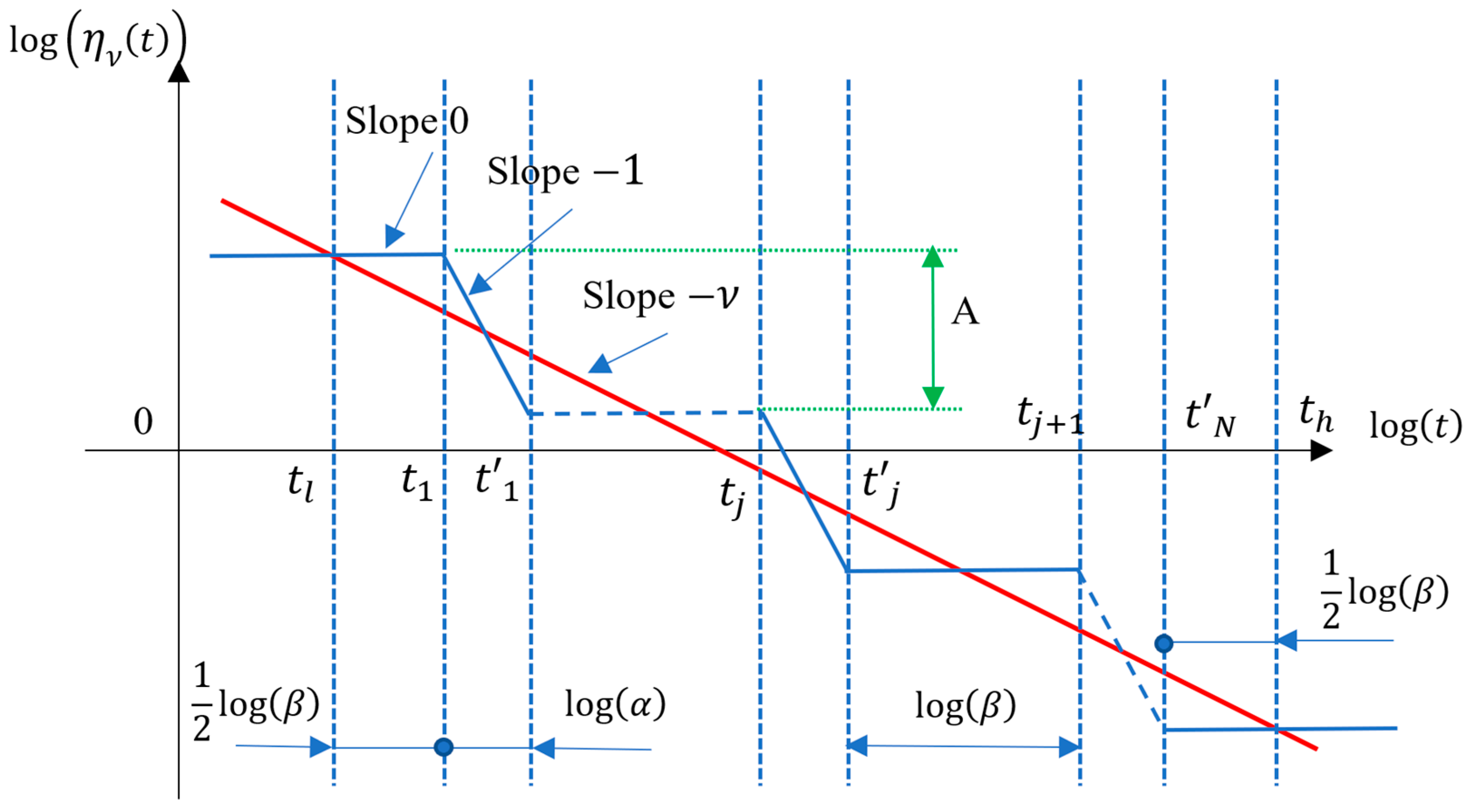
1—Choose and and the number of intervals of which the function is sampled in Figure 9. 2—Compute , and the times and , 3—Compute the gain so that for (namely the middle of the interval ) thus for : | |
5. Conclusions
- without requiring classical fractional calculus operators.
- using non singular kernels.
Funding
Data Availability Statement
Conflicts of Interest
References
- Sabatier, J.; Farges, C.; Tartaglione, V. Fractional Behaviours Modelling: Analysis and Application of Several Unusual Tools; Intelligent Systems, Control and Automation: Science and Engineering series; Springer: Cham, Switzerland, 2022; Volume 101. [Google Scholar]
- Samko, S.G.; Kilbas, A.A.; Marichev, O.I. Fractional Integrals and Derivatives: Theory and Applications; Gordon and Breach Science Publishers: London, UK, 1993. [Google Scholar]
- Podlubny, I. Fractional Differential Equations. Theoretical Developments and Applications in Physics and Engineering Mathematics in Sciences and Engineering; Academic Press: Cambridge, MA, USA, 1999. [Google Scholar]
- Miller, K.; Ross, B. An Introduction to the Fractional Calculus and Fractional Differential Equations; John Wiley & Sons Inc.: Hoboken, NJ, USA, 1993. [Google Scholar]
- Monje, C.A.; Chen, Y.; Vinagre, B.M.; Xue, D.; Feliu, V. Fractional-Order Systems and Controls: Fundamentals and Applications; Advances in Industrial Control Series; Springer: London, UK, 2010. [Google Scholar]
- Baleanu, D.; Balas, V.E.; Agarwal, P. Fractional Order Systems and Applications in Engineering; Elsevier: Amsterdam, The Netherlands, 2022. [Google Scholar]
- Petras, I. Fractional Order Systems; MDPI Books: Basel, Switzerland, 2019. [Google Scholar]
- Dokoumetzidis, A.; Magin, R.; Macheras, P. A commentary on fractionalization of multi-compartmental models. Pharm. Pharm. 2010, 37, 203–207. [Google Scholar] [CrossRef] [PubMed]
- Sabatier, J.; Farges, C.; Trigeassou, J.C. Fractional systems state space description: Some wrong ideas and proposed solutions. J. Vib. Control 2014, 20, 1076–1084. [Google Scholar] [CrossRef]
- Balint, A.M.; Balint, S. Mathematical Description of the Groundwater Flow and that of the Impurity Spread, Which Use Temporal Caputo or Riemann-Liouville Fractional Partial Derivatives, Is Non-objective. Fractal Fract. 2020, 4, 36. [Google Scholar] [CrossRef]
- Pantokratoras, A. Comment on the paper “Fractional order model of thermo-solutal and magnetic nanoparticles transport for drug delivery applications, Subrata Maiti, Sachin Shaw, G.C. Shit”. Colloids Surf. B Biointerfaces 2023, 222, 113074. [Google Scholar] [CrossRef]
- Sabatier, J. Solutions to the Sub-Optimality and Stability Issues of Recursive Pole and Zero Distribution Algorithms for the Approximation of Fractional Order Models. Algorithms 2018, 11, 103. [Google Scholar] [CrossRef]
- Stynes, M. Fractional-order derivatives defined by continuous kernels are too restrictive. Appl. Math. Lett. 2018, 85, 22–26. [Google Scholar] [CrossRef]
- Hanyga, A. A comment on a controversial issue: A generalized fractional derivative cannot have a regular kernel. Fract. Calc. Appl. Anal. 2020, 23, 211–223. [Google Scholar] [CrossRef]
- Kai Diethelm, K.; Garrappa, R.; Giusti, A.; Stynes, M. Why fractional derivatives with nonsingular kernels should not be used. Fract. Calc. Appl. Anal. 2020, 23, 610–634. [Google Scholar] [CrossRef]
- Sabatier, J. Fractional-Order Derivatives Defined by Continuous Kernels: Are They Really Too Restrictive? Fractal Fract. 2020, 4, 40. [Google Scholar] [CrossRef]
- Sabatier, J.; Merveillaut, M.; Malti, R.; Oustaloup, A. How to impose physically coherent initial conditions to a fractional system? Commun. Nonlinear Sci. Numer. Simul. 2010, 15, 1318–1326. [Google Scholar] [CrossRef]
- Ortigueira, M.D.; Coito, F. System initial conditions vs derivative initial conditions. Comput. Math. Appl. 2010, 59, 1782–1789. [Google Scholar] [CrossRef]
- Sabatier, J. Fractional Order Models Are Doubly Infinite Dimensional Models and thus of Infinite Memory: Consequences on Initialization and Some Solutions. Symmetry 2021, 13, 1099. [Google Scholar] [CrossRef]
- Sun, H.; Wang, Y.; Yu, L.; Yu, X. A discussion on nonlocality: From fractional derivative model to peridynamic model. Commun. Nonlinear Sci. Numer. Simul. 2022, 114, 106604. [Google Scholar] [CrossRef]
- Caputo, M.; Fabrizio, M. A new definition of fractional derivative without singular kernel. Prog. Fract. Differ. Appl. 2015, 1, 73–85. [Google Scholar]
- Arshad, S.; Saleem, I.; Akgül, A.; Huang, J.; Tang, Y.; Eldin, S.M. A novel numerical method for solving the Caputo-Fabrizio fractional differential equation. AIMS Math. 2023, 8, 9535–9556. [Google Scholar] [CrossRef]
- Hristov, J. Derivatives with Non-Singular Kernels from the Caputo-Fabrizio Definition and Beyond: Appraising Analysis with Emphasis on Diffusion Models. Curr. Dev. Math. Sci. Front. Fract. Calc. 2018, 1, 269. [Google Scholar] [CrossRef]
- Yépez-Martínez, H.; Gómez-Aguilar, J.F. A new modified definition of Caputo–Fabrizio fractional-order derivative and their applications to the Multi Step Homotopy Analysis Method (MHAM). J. Comput. Appl. Math. 2019, 346, 247–260. [Google Scholar] [CrossRef]
- Alshabanat, A.; Jleli, M.; Kumar, S.; Samet, B. Generalization of Caputo-Fabrizio Fractional Derivative and Applications to Electrical Circuits. Front. Phys. Sec. Stat. Comput. Phys. 2020, 8, 64. [Google Scholar] [CrossRef]
- Qureshi, S.; Rangaig, N.A.; Baleanu, D. New Numerical Aspects of Caputo-Fabrizio Fractional Derivative Operator. Mathematics 2019, 7, 374. [Google Scholar] [CrossRef]
- Ali, F.; Ali, F.; Sheikh, N.A.; Khan, I.; Nisar, K.S. Caputo–Fabrizio fractional derivatives modeling of transient MHD Brinkman nanoliquid: Applications in food technology. Chaos Solitons Fractals 2020, 131, 109489. [Google Scholar] [CrossRef]
- Atangana, A.; Baleanu, D. New fractional derivatives with nonlocal and non-singular kernel: Theory and application to heat transfer model. Therm. Sci. 2016, 20, 763–769. [Google Scholar] [CrossRef]
- Liemert, A.; Sandev, T.; Kantz, H. Generalized langevin equation with tempered memory kernel. Phys. A—Stat. Mech. Appl. 2017, 466, 356–369. [Google Scholar] [CrossRef]
- Hattaf, K. A new generalized definition of fractional derivative with non-singular kernel. Computation 2020, 8, 49. [Google Scholar] [CrossRef]
- Al-Refai, M. Proper inverse operators of fractional derivatives with nonsingular kernels. Rend. Circ. Mat. Palermo, II Ser. 2022, 71, 525–535. [Google Scholar] [CrossRef]
- Yusuf, A.; Inc, M.; Aliyu, A.I.; Baleanu, D. Efficiency of the new fractional derivative with nonsingular Mittag-Leffler kernel to some nonlinear partial differential equations. Chaos Solitons Fractals 2018, 116, 202–226. [Google Scholar] [CrossRef]
- Fernandez, A.; Al-Refai, M. A Rigorous Analysis of Integro-Differential Operators with Non-Singular Kernels. Fractal Fract. 2023, 7, 213. [Google Scholar] [CrossRef]
- Sabatier, J.; Farges, C. Algorithms for Fractional Dynamical Behaviors Modelling Using Non-Singular Rational Kernels. Algorithms 2024, 17, 20. [Google Scholar] [CrossRef]
- Sabatier, J.; Farges, C. Time-Domain Fractional Behaviour Modelling with Rational Non-Singular Kernels. Axioms 2024, 13, 99. [Google Scholar] [CrossRef]
- Manabe, S. The non-integer Integral and its Application to control systems. ETJ Jpn. 1961, 6, 83–87. [Google Scholar]
- Carlson, G.E.; Halijak, C.A. Simulation of the Fractional Derivative Operator and the Fractional Integral Operator. Available online: http://krex.k-state.edu/dspace/handle/2097/16007 (accessed on 1 December 2024).
- Ichise, M.; Nagayanagi, Y.; Kojima, T. An analog simulation of non-integer order transfer functions for analysis of electrode processes. J. Electroanal. Chem. Interfacial Electrochem. 1971, 33, 253–265. [Google Scholar] [CrossRef]
- Oustaloup, A. Systèmes Asservis Linéaires d’ordre Fractionnaire; Masson: Paris, France, 1983. [Google Scholar]
- Raynaud, H.F.; Zergaïnoh, A. State-space representation for fractional order controllers. Automatica 2000, 36, 1017–1021. [Google Scholar] [CrossRef]
- Charef, A. Analogue realisation of fractional-order integrator, differentiator and fractional PIλDµ controller. IEE Proc. Control Theory Appl. 2006, 153, 714–720. [Google Scholar] [CrossRef]
- Nigmatullin, R.R.; Arbuzov, A.A.; Salehli, F.; Giz, A.; Bayrak, I.; Catalgil-Giz, H. The first experimental confirmation of the fractional kinetics containing the complex-power-law exponents: Dielectric measurements of polymerization reactions. Phys. B Condens. Matter 2007, 388, 418–434. [Google Scholar] [CrossRef]


Disclaimer/Publisher’s Note: The statements, opinions and data contained in all publications are solely those of the individual author(s) and contributor(s) and not of MDPI and/or the editor(s). MDPI and/or the editor(s) disclaim responsibility for any injury to people or property resulting from any ideas, methods, instructions or products referred to in the content. |
© 2025 by the author. Licensee MDPI, Basel, Switzerland. This article is an open access article distributed under the terms and conditions of the Creative Commons Attribution (CC BY) license (https://creativecommons.org/licenses/by/4.0/).
Share and Cite
Sabatier, J. Fractional Dynamical Behaviour Modelling Using Convolution Models with Non-Singular Rational Kernels: Some Extensions in the Complex Domain. Fractal Fract. 2025, 9, 79. https://doi.org/10.3390/fractalfract9020079
Sabatier J. Fractional Dynamical Behaviour Modelling Using Convolution Models with Non-Singular Rational Kernels: Some Extensions in the Complex Domain. Fractal and Fractional. 2025; 9(2):79. https://doi.org/10.3390/fractalfract9020079
Chicago/Turabian StyleSabatier, Jocelyn. 2025. "Fractional Dynamical Behaviour Modelling Using Convolution Models with Non-Singular Rational Kernels: Some Extensions in the Complex Domain" Fractal and Fractional 9, no. 2: 79. https://doi.org/10.3390/fractalfract9020079
APA StyleSabatier, J. (2025). Fractional Dynamical Behaviour Modelling Using Convolution Models with Non-Singular Rational Kernels: Some Extensions in the Complex Domain. Fractal and Fractional, 9(2), 79. https://doi.org/10.3390/fractalfract9020079