Dynamic Analysis of a 10-Dimensional Fractional-Order Hyperchaotic System Using Advanced Hyperchaotic Metrics

Abstract

In this paper, we propose an innovative approach to fractional-order dynamics by introducing a 10-dimensional (10D) chaotic system that leverages the intrinsic memory characteristic of the Grünwald–Letnikov (G-L) derivative. We utilize Lyapunov exponents as a quantitative measure to characterize hyperchaotic behavior, and classify the nature of the suggested 10D fractional-order system (FOS). While several methods exist for calculating Lyapunov exponents (LEs) through the utilization of integer-order systems, these approaches are not applicable for FOS due to its non-local nature. Initially, the system dynamics are thoroughly examined through Lyapunov exponents and bifurcation analysis, considering the influence of both state variables and fractional orders. To assess the hyperchaotic behavior of the proposed model, sensitivity analyses are conducted by exploring changes in state variables under two distinct initial conditions, along with time history simulations for various parameter settings. Furthermore, we examine the impact of different fractional-order sets on the system’s dynamics. A comprehensive performance comparison is conducted between the proposed 10-dimensional fractional-order hyperchaotic system and several existing hyperchaotic systems. This comparison utilizes advanced metrics, including the Kolmogorov–Sinai (KS) entropy, Kaplan–Yorke dimension, the Perron effect analysis, and the 0-1 test for chaos. Simulation outcomes reveal that the proposed system surpasses existing algorithms, delivering improved precision and accuracy.

1. Introduction

Chaos is a pseudo-random phenomenon arising from deterministic dynamical systems, characterized by unpredictability, nonlinearity, and extreme sensitivity to initial conditions. Chaotic systems are ubiquitous in both natural and artificial environments. Since the Lorenz system was introduced as the first chaotic model [1], chaos theory has attracted considerable attention, inspiring researchers to investigate its intricate dynamics. Beyond theoretical exploration, chaotic systems have found extensive applications in various practical engineering domains, including atmospheric science, neural networks, ecological modeling, secure communication, and synchronization control [2,3,4,5]. The intrinsic complexity and versatility of chaotic system dynamics often dictate their practical relevance, driving ongoing research aimed at designing systems with enhanced and diversified dynamical behaviors.

In recent years, the study of concealed chaos has garnered significant attention. Traditionally, chaotic system attractors have been classified into two categories: self-excited attractors and hidden attractors. A hidden attractor, considered a distinct and innovative type of attractor, was first identified in the classical Chua circuit [6]. Unlike conventional homoclinic attractors [7], such as the Chen attractor [8] and the Lorenz attractor [1], hidden attractors are distinguished by basins of attraction that do not intersect with the neighborhood of any unstable equilibrium point. These attractors can arise in three types of chaotic systems: those with an infinite number of equilibrium points [9], those with stable equilibrium points [10], and those entirely devoid of equilibria [11].

The Lyapunov exponent (LE), also known as the Lyapunov characteristic exponent, is a mathematical metric used to quantify the rate of divergence between two trajectories that originate infinitesimally close to each other within a dynamical system. This measure plays a crucial role in assessing the predictability of a system. The largest Lyapunov exponent (LLE), often referred to as the maximal Lyapunov exponent (MLE), serves as a key indicator of chaotic behavior. A positive MLE signifies the presence of chaos within the system, while a system with at least one positive LE is classified as chaotic. On the other hand, hyperchaotic systems are characterized by having more than one positive LE, which implies that their chaotic dynamics evolve in multiple directions simultaneously. Consequently, hyperchaotic systems exhibit greater dynamical complexity than traditional chaotic systems, making them particularly advantageous for enhancing the security of unpredictable communication systems.

The exploration of chaotic behavior in both fractional-order and integer-order systems has become a significant focus within dynamical systems research. Chaotic dynamics, defined by their high sensitivity to initial conditions and inherent unpredictability over time, are integral to numerous applications such as cryptography, secure communication, and various branches of the physical sciences [1,2]. While traditional chaotic systems are commonly modeled using integer-order DEs, there is an increasing interest in FO chaotic systems. These systems, utilizing derivatives of non-integer orders, have proven to be more effective in capturing and modeling the intricacies of complex real-world phenomena [12].

ODEs systems have been extended in recent years to encompass fractional differential equations (FDEs), offering a broader and more versatile mathematical framework. FDEs are widely recognized for their ability to enhance the accuracy of modeling complex systems, particularly those that exhibit memory and hereditary properties. Furthermore, FDEs are believed to have the potential to reduce computational costs compared to traditional ODEs, making them a promising alternative for achieving more efficient and precise solutions across various applications.

The Riemann–Liouville fractional derivative, a well-known classical approach to fractional calculus, is characterized for a function $f\left(t\right)$ of order $\beta >0$ as follows [13]:

$$\begin{array}{c}\hfill D_t^{\beta }\eta \left(t\right)={\displaystyle \frac{1}{\Gamma (n-\beta )}}{\displaystyle \frac{d^n}{d{t}^n}}{\int }_a^t{\displaystyle \frac{\eta \left(\tau \right)}{{(t-\tau )}^{\beta -n+1}}}d\tau ,\end{array}$$

where $\Gamma (·)$ denotes the Gamma function, expressed as $\Gamma \left(u\right)={\int }_0^{\infty }{x}^{u-1}{e}^{-x}dx$. The parameter $n=\lceil \beta \rceil$ represents the smallest integer not less than $\beta$, and a signifies the lower bound of the integral, typically set to 0 or $-\infty$.

The conformable derivative presented in [14] of a mapping $\eta \left(t\right)$ of fractional order $\beta$ is given by

$$T_{\beta }\left(\eta \right)\left(t\right)=\underset{ϵ\to 0}{lim}{\displaystyle \frac{\eta (t+ϵt^{1-\beta })-\eta \left(t\right)}{ϵ}}.$$

On the other hand, it can be expressed as

$$T_{\beta }\left(\eta \right)\left(t\right)=t^{1-\beta }{\displaystyle \frac{d\eta \left(t\right)}{dt}},t>0,\beta \in (0,1],$$

where $\beta$ denotes the FO of the presented derivative, with $0<\beta \le 1$, $ϵ$ represents an infinitesimal increment, and $t^{1-\beta }$ modifies the ordinary derivative to reflect the FO.

The fractional derivative introduced by Atangana and Baleanu [15], defined in the Caputo framework, is expressed as

$$\begin{array}{c}\hfill {}^{\mathit{ABC}}D_t^{\beta }\eta \left(t\right)={\displaystyle \frac{M\left(\beta \right)}{1-\beta }}{\int }_0^t{E}_{\beta }\left(-{\displaystyle \frac{\beta {(t-\tau )}^{\beta }}{1-\beta }}\right){\displaystyle \frac{d\eta \left(\tau \right)}{d\tau }}d\tau ,(0<\beta <1),\end{array}$$

where $M\left(\beta \right)=1-\beta$ and the Mittag–Leffler mapping is presented by

$$\begin{array}{c}\hfill E_{\beta }\left(u\right)=\sum _{k=0}^{\infty }{\displaystyle \frac{u^k}{\Gamma (\beta k+1)}},\end{array}$$

where u represents the input parameter of the Mittag–Leffler mapping.

FODs stand out from integer-order derivatives due to their inherent non-local behavior and memory-dependent properties. These unique features enable FOS to display significantly richer and more intricate dynamics compared to traditional integer-order systems [16]. Among the many definitions of fractional derivatives, the G-L derivative is especially noteworthy for its discrete formulation, which simplifies its numerical implementation, making it highly advantageous for simulating chaotic systems [17,18].

The G-L derivative serves as a cornerstone in fractional calculus, generalizing the conventional idea of differentiation to FOs. This derivative is derived by modifying the traditional limit definition of differentiation and integrating a fractional-order integral operator. A comprehensive discrete framework is introduced for numerically solving complex, nonlinear, and time-dependent fractional parabolic equations, employing the G-L derivative approach for temporal discretization [19].

The fractional derivative of a function $\eta :\mathbb{R}\to \mathbb{R}$, as defined using the G-L approach, is given by

$$\begin{array}{c}\hfill D^{\beta }\eta \left(x\right)=\underset{h\to 0}{lim}{\displaystyle \frac{1}{h^{\beta }}}\sum _{r=0}^{\infty }{(-1)}^r\left({\displaystyle \genfrac{}{}{0pt}{}{\beta }{r}}\right)\eta (x-rh),\end{array}$$

where $\left({\displaystyle \genfrac{}{}{0pt}{}{\beta }{r}}\right)$ denotes the generalized binomial coefficient for fractional orders $\beta$, and it is expressed as

$$\begin{array}{c}\hfill \left({\displaystyle \genfrac{}{}{0pt}{}{\beta }{r}}\right)={\displaystyle \frac{\beta (\beta -1)\cdots (\beta -r+1)}{r!}}.\end{array}$$

This definition offers a versatile approach, broadening the scope of classical derivatives by incorporating a summation of increments h scaled by fractional exponents. It provides a valuable tool for studying functions with behaviors that cannot be adequately described using standard integer-order derivatives. One notable strength of this method is its ability to demonstrate how fractional-order parameters, such as $\beta$, can substantially affect both the precision of numerical solutions and the associated computational effort [20]. Additionally, numerous studies have explored the implementation of FODs in various models, as highlighted in [21,22] and related works.

LEs are essential for understanding dynamical systems, as they measure how rapidly nearby trajectories diverge, offering critical information about the system’s stability and chaotic dynamics. However, determining LEs in fractional-order systems is particularly challenging because of the inherent non-local characteristics of fractional derivatives, making traditional methods for integer-order systems unsuitable [23].

In Chua’s revised system incorporating fractional derivatives, the equations governing the system include terms with FODs are formulated as

$$\begin{array}{cc}\hfill D^{\beta }{x}_1& =a_1(x_2-h\left(x_1\right)),\hfill \\ \hfill D^{\beta }{x}_2& =x_1-x_2+x_3,\hfill \\ \hfill D^{\beta }{x}_3& =-a_2{x}_2.\hfill \end{array}$$

The nonlinear function $h\left(x_1\right)$, representing the behavior of Chua’s diode, is mathematically expressed as

$$\begin{array}{c}\hfill h\left(x_1\right)=b_1{x}_1+{\displaystyle \frac{1}{2}}(b_0-b_1)\left(\right|x_1+1|-|x_1-1\left|\right),\end{array}$$

The constants $b_0$ and $b_1$ define the piecewise-linear properties of the diode. To achieve the desired dynamical characteristics and ensure stability, the system parameters $a_1$, $a_2$, $b_0$, and $b_1$ must be appropriately chosen. Furthermore, the initial values of the state variables $x_1$, $x_2$, and $x_3$ need to be specified for accurately modeling the system’s dynamics.

The regulation of chaotic behavior has become a prominent focus in recent research. This heightened interest stems from the study of chaotic systems using diverse mathematical and physical frameworks, including the fractional-order model proposed by Chen [8]. By incorporating fractional derivatives defined according to the Caputo framework, the traditional Chen system has been transformed into its fractional-order counterpart.

FO Chen’s system represents a generalized form of the classical Chen system, where the conventional integer-order derivatives are substituted with FO derivatives. This alteration provides various benefits:

• The integration of fractional-order derivatives into the Chen system provides a generalized framework that enables the modeling of a wider spectrum of dynamic behaviors. This extension enhances its relevance in various domains where nonlocal memory effects are critical for accurate representation.
• FO operators offer a more versatile and precise approach to representing memory and hereditary characteristics inherent in numerous real-world phenomena. Unlike traditional integer-order models that emphasize local interactions, FO models incorporate the complete historical behavior of state variables, allowing for more accurate simulation of systems with long-term temporal dependencies.
• The inclusion of fractional-order derivatives introduces greater complexity to the system’s dynamics, resulting in a broader array of bifurcation patterns and chaotic attractors. This increased complexity makes the FO Chen system more capable of describing intricate chaotic phenomena encountered in fields such as physics, biology, and engineering.
• The FO Chen system demonstrates chaotic dynamics at lower parameter thresholds compared to its classical counterpart. This property is particularly beneficial for applications relying on chaos, such as secure communication in cryptography and efficient random number generation.

The updated system can be represented using the equations below:

$$\begin{array}{cc}\hfill D^{\beta }x& =a_1(y-x),\hfill \\ \hfill D^{\beta }y& =(a_3-a_1)x-xz+a_{3}y,\hfill \\ \hfill D^{\beta }z& =xy-a_{2}z,\hfill \end{array}$$

where $a_1$, $a_2$, and $a_3$ are constants that characterize the system, and $\beta$ represents the order of the fractional derivatives, satisfying $0<\beta \le 1$.

This research article introduces a novel approach to FO dynamics within a 10-dimensional framework. By integrating these dynamics, the presented system demonstrates a broader range of dynamical behaviors. We validate the effectiveness of our methodology by applying it to a 10D FO Chen system, showcasing its potential for generating hyperchaotic systems.

In this work, we introduce a novel 10D hyperchaotic system formulated using the classical differential operator, described as follows:

$$\begin{array}{cc}\hfill {\dot{x}}_1& ={\sigma }_1(x_2-x_1)+x_4,\hfill \\ \hfill {\dot{x}}_2& ={\sigma }_2{x}_1-x_1{x}_3+x_4,\hfill \\ \hfill {\dot{x}}_3& =x_1{x}_2-x_3-x_4+x_7,\hfill \\ \hfill {\dot{x}}_4& ={\sigma }_3(x_1+x_2)+x_5,\hfill \\ \hfill {\dot{x}}_5& =-x_2-{\sigma }_4{x}_4+x_6,\hfill \\ \hfill {\dot{x}}_6& =-{\sigma }_5(x_1+x_5)+{\sigma }_4{x}_7,\hfill \\ \hfill {\dot{x}}_7& =-{\sigma }_6(x_1+x_6-x_8),\hfill \\ \hfill {\dot{x}}_8& =-{\sigma }_7{x}_{10},\hfill \\ \hfill {\dot{x}}_9& ={\sigma }_8(x_2-x_1)+x_4-x_5-x_6,\hfill \\ \hfill {\dot{x}}_{10}& ={\sigma }_9{x}_1-x_2-x_1{x}_3,\hfill \end{array}$$

(1)

where $x_1,x_2,\dots ,x_9$ and $x_{10}$ are the state vectors and ${\sigma }_1,{\sigma }_2,\dots ,{\sigma }_9$ are constant parameters. The following sections will explore various dynamical properties of the system defined by Equation (1).

To investigate the underlying hyperchaotic system, we employ the Grünwald–Letnikov (G-L) derivative to analyze the presented model. The FOS, characterized by its hereditary and memory effects, is generally considered more advantageous than the integer-order system. In the study of FDEs, both the Riemann–Liouville and the Caputo derivatives are widely utilized. However, the Grünwald–Letnikov (G-L) derivative is often preferred because it retains the same initial conditions as integer-order differential equations. In contrast, the Riemann–Liouville operator requires nonlocal or fractional initial conditions, which complicates the analysis. While integer-order systems offer limited options, fractional-order systems provide greater flexibility and exhibit a richer variety of dynamical behaviors due to the fractional-order parameter.

Ben Makhlouf and El-Hady proposed new insights into the stability of Caputo FDEs in their study [24]. Fractional operators have been utilized to study hidden attractors in chaotic dynamical systems, facilitating the emergence of new chaotic behaviors. N. Sene analyzed hidden chaotic dynamics in fractional-order systems governed by Caputo fractional differential equations [25]. Gao et al. analyzed a novel hyperchaotic system that incorporates a fractional operator [26]. Moreover, numerous hidden attractors have been explored within hyperchaotic systems utilizing FO operators [27,28,29]. Given that fractional operators preserve memory and exhibit nonlocal kernels, hidden attractors can be explored at fractional-orders within the range (0, 1], which is not feasible with integer orders.

The study of multi-term fractional-order differential equations (FDEs) and their qualitative behaviors is closely related to the analysis of multi-order systems of fractional differential equations. A comprehensive discussion of this connection can be found in [30]. Research into the stability characteristics of multi-term FDEs has primarily focused on equations with two or three fractional terms, as explored in recent works such as [31,32]. However, due to the heightened complexity involved, equations incorporating four or more fractional terms remain largely unexplored. For further insights into multi-term FDEs, refer to [33].

This paper is structured as follows: Section 1 provides an overview of fractional-order differential equations, the Grünwald–Letnikov (G-L) approach, and various related systems discussed in previous studies.

Section 2 introduces the proposed mathematical model for the 10-dimensional fractional-order system, utilizing the G-L derivative for calculations. The numerical simulations and analysis of the proposed system, based on this methodology, are presented in Section 3. This section includes a comprehensive exploration of the 10-dimensional fractional-order system for $t=200$, featuring subsections dedicated to analyzing hyperchaotic behavior using Lyapunov exponents (LEs) and the bifurcations of state variables through variations in parameters and fractional-orders. Additionally, a sensitivity analysis is conducted, and both 2D and 3D Poincaré sections are employed to further investigate the hyperchaotic dynamics.

Section 4 focuses on the complexity analysis of the system, encompassing methods such as the Perron effect, Kolmogorov–Sinai (KS) entropy, the Kaplan–Yorke (KY) fractal dimension, and analysis of the 0-1 Test for chaos. Section 6 provides an in-depth discussion of the results obtained, while Section 7 summarizes the key findings of the study. Finally, Section 8 presents potential future applications of the proposed methods.

2. Mathematical Model and Computational Technique

2.1. Basic Idea

The proposed algorithm is based on the discretization of a continuous-time system using numerical methods designed for FDEs. The time-dependent evolution of small initial perturbations is described as a discrete function that tracks changes in system deviations. The LE is calculated as the average logarithmic rate of divergence of these perturbations. To determine the complete spectrum of LEs, individual dimensions of the system are perturbed, and the Gram–Schmidt orthonormalization technique is employed to counteract numerical instabilities caused by positive LEs.

The suggested 10D Chen system, formulated through fractional-order DEs, is described by the following FO system:

$$\begin{array}{cc}\hfill D_t^{{\beta }_1}{x}_1& ={\mathbf{\Phi }}_1={\sigma }_1(x_2-x_1)+x_4,\hfill \\ \hfill D_t^{{\beta }_2}{x}_2& ={\mathbf{\Phi }}_2={\sigma }_2{x}_1-x_1{x}_3+x_4,\hfill \\ \hfill D_t^{{\beta }_3}{x}_3& ={\mathbf{\Phi }}_3=x_1{x}_2-x_3-x_4+x_7,\hfill \\ \hfill D_t^{{\beta }_4}{x}_4& ={\mathbf{\Phi }}_4={\sigma }_3(x_1+x_2)+x_5,\hfill \\ \hfill D_t^{{\beta }_5}{x}_5& ={\mathbf{\Phi }}_5=-x_2-{\sigma }_4{x}_4+x_6,\hfill \\ \hfill D_t^{{\beta }_6}{x}_6& ={\mathbf{\Phi }}_6=-{\sigma }_5(x_1+x_5)+{\sigma }_4{x}_7,\hfill \\ \hfill D_t^{{\beta }_7}{x}_7& ={\mathbf{\Phi }}_7=-{\sigma }_6(x_1+x_6-x_8),\hfill \\ \hfill D_t^{{\beta }_8}{x}_8& ={\mathbf{\Phi }}_8=-{\sigma }_7{x}_{10},\hfill \\ \hfill D_t^{{\beta }_9}{x}_9& ={\mathbf{\Phi }}_9={\sigma }_8(x_2-x_1)+x_4-x_5-x_6,\hfill \\ \hfill D_t^{{\beta }_{10}}{x}_{10}& ={\mathbf{\Phi }}_{10}={\sigma }_9{x}_1-x_2-x_1{x}_3,\hfill \end{array}$$

(2)

where every ${\beta }_m$ (for each $m=1,2,\dots ,10$) satisfies $0<{\beta }_m<1$. Moreover, a real-valued 10D vector mapping is defined as $\mathbf{\Phi }\left(\mathbf{x}\right)={({\mathbf{\Phi }}_1\left(\mathbf{x}\right),{\mathbf{\Phi }}_2\left(\mathbf{x}\right),\dots ,{\mathbf{\Phi }}_{10}\left(\mathbf{x}\right))}^T$, where $\mathbf{x}={(x_1,x_2,\dots ,x_{10})}^T\in {\mathbb{R}}^{10}$. The term $D_t^{{\beta }_m}$ represents the Grünwald–Letnikov FOD operator for $0<{\beta }_m<1$. Moreover, the parameters ${\sigma }_1,{\sigma }_2,\dots ,{\sigma }_9$ are constants that determine the dynamics of the proposed 10D FOS (2).

The Lyapunov exponent, denoted by $\lambda$, is commonly known as the mean logarithmic rate at which small perturbations in a system’s trajectory exponentially diverge, i.e.,

$$\begin{array}{c}\hfill \lambda =\underset{t\to \infty }{lim}{\displaystyle \frac{1}{t}}ln{\displaystyle \frac{\parallel q\left(t\right)\parallel }{\parallel q\left(t_0\right)\parallel }},\end{array}$$

(3)

where the initial perturbation, $\mathbf{q}\left(t_0\right)$, which induces a divergence occurring in the evolution of two phase trajectories, is commonly represented as

$$\begin{array}{c}\hfill {\mathbf{q}}^{\prime }={\mathbf{J}}_{\mathbf{\Phi }}\mathbf{q},\end{array}$$

(4)

$$\begin{array}{c}\hfill \mathbf{q}\left(t_0\right)=\mathbf{x}\left(t_0\right)-\overline{\mathbf{x}}\left(t_0\right),\end{array}$$

(5)

where $\mathbf{\Phi }\left(\mathbf{x}\right)$ in the form of Jacobian matrix is expressed as ${\mathbf{J}}_{\mathbf{\Phi }}={\displaystyle \frac{d\mathbf{\Phi }}{d\mathbf{x}}}$.

In this article, we introduce a new technique for computing all LEs for FOS, as described in Equation (2). This technique incorporates the method proposed by Grünwald [17] and the fractional decomposition technique proposed by Letnikov [18]. Additionally, it involves solving Equations (4) and (5), since the LE is defined through Equation (3). The deviation, represented as $\mathbf{q}$, cannot be expressed using Equations (4) and (5) because of the nonlocal characteristics inherent in the FOS.

2.2. Development of the Proposed Method

The study explores the fractional-order extension of the 10D ODE system presented in Equations (2). A numerical approach is formulated by leveraging the memory principle derived from the Grünwald–Letnikov definition. Within this framework, the approach is treated as a 10D mapping, which is defined by its distinct characteristics, i.e.,

$$\begin{array}{c}\hfill \mathbf{x}\left(t_{\mu +1}\right)=\mathbf{H}(\mathbf{x}\left(t_{\mu }\right),t_{\mu }),\end{array}$$

(6)

where $t_{\mu }=\mu h$, h is a time-step, and $\mathbf{H}={({\mathbf{H}}_1,{\mathbf{H}}_2,\dots ,{\mathbf{H}}_{10})}^T$; then, utilizing the proposed method of Grünwald–Letnikov on 10D FOS (2), we can establish ${\mathbf{H}}_1,{\mathbf{H}}_2,\dots ,{\mathbf{H}}_{10}$ as follows:

$$\begin{array}{cc}\hfill {\mathbf{H}}_1(\mathbf{x}\left(t_{\mu }\right),t_{\mu })& =\left({\sigma }_1(x_2\left(t_{\mu }\right)-x_1\left(t_{\mu }\right))+x_4\left(t_{\mu }\right)\right)h^{{\beta }_1}-\sum _{\nu =1}^{\mu +1}{C}_{\nu }^{\left({\beta }_1\right)}{x}_1\left(t_{\mu +1-\nu }\right),\hfill \\ \hfill {\mathbf{H}}_2(\mathbf{x}\left(t_{\mu }\right),t_{\mu })& =\left({\sigma }_2{x}_1\left(t_{\mu }\right)-x_1\left(t_{\mu }\right)x_3\left(t_{\mu }\right)+x_4\left(t_{\mu }\right)\right)h^{{\beta }_2}-\sum _{\nu =1}^{\mu +1}{C}_{\nu }^{\left({\beta }_2\right)}{x}_2\left(t_{\mu +1-\nu }\right),\hfill \\ \hfill {\mathbf{H}}_3(\mathbf{x}\left(t_{\mu }\right),t_{\mu })& =\left(x_1\left(t_{\mu }\right)x_2\left(t_{\mu }\right)-x_3\left(t_{\mu }\right)-x_4\left(t_{\mu }\right)+x_7\left(t_{\mu }\right)\right)h^{{\beta }_3}-\sum _{\nu =1}^{\mu +1}{C}_{\nu }^{\left({\beta }_3\right)}{x}_3\left(t_{\mu +1-\nu }\right),\hfill \\ \hfill {\mathbf{H}}_4(\mathbf{x}\left(t_{\mu }\right),t_{\mu })& =\left({\sigma }_3(x_1\left(t_{\mu }\right)+x_2\left(t_{\mu }\right))+x_5\left(t_{\mu }\right)\right)h^{{\beta }_4}-\sum _{\nu =1}^{\mu +1}{C}_{\nu }^{\left({\beta }_4\right)}{x}_4\left(t_{\mu +1-\nu }\right),\hfill \\ \hfill {\mathbf{H}}_5(\mathbf{x}\left(t_{\mu }\right),t_{\mu })& =\left(-x_2\left(t_{\mu }\right)-{\sigma }_4{x}_4\left(t_{\mu }\right)+x_6\left(t_{\mu }\right)\right)h^{{\beta }_5}-\sum _{\nu =1}^{\mu +1}{C}_{\nu }^{\left({\beta }_5\right)}{x}_5\left(t_{\mu +1-\nu }\right),\hfill \\ \hfill {\mathbf{H}}_6(\mathbf{x}\left(t_{\mu }\right),t_{\mu })& =\left(-{\sigma }_5(x_1\left(t_{\mu }\right)+x_5\left(t_{\mu }\right))+{\sigma }_4{x}_7\left(t_{\mu }\right)\right)h^{{\beta }_6}-\sum _{\nu =1}^{\mu +1}{C}_{\nu }^{\left({\beta }_6\right)}{x}_6\left(t_{\mu +1-\nu }\right),\hfill \\ \hfill {\mathbf{H}}_7(\mathbf{x}\left(t_{\mu }\right),t_{\mu })& =\left(-{\sigma }_6(x_1\left(t_{\mu }\right)+x_6\left(t_{\mu }\right)-x_8\left(t_{\mu }\right))\right)h^{{\beta }_7}-\sum _{\nu =1}^{\mu +1}{C}_{\nu }^{\left({\beta }_7\right)}{x}_7\left(t_{\mu +1-\nu }\right),\hfill \\ \hfill {\mathbf{H}}_8(\mathbf{x}\left(t_{\mu }\right),t_{\mu })& =\left(-{\sigma }_7{x}_{10}\left(t_{\mu }\right)\right)h^{{\beta }_8}-\sum _{\nu =1}^{\mu +1}{C}_{\nu }^{\left({\beta }_8\right)}{x}_8\left(t_{\mu +1-\nu }\right),\hfill \\ \hfill {\mathbf{H}}_9(\mathbf{x}\left(t_{\mu }\right),t_{\mu })& =\left({\sigma }_8(x_2\left(t_{\mu }\right)-x_1\left(t_{\mu }\right))+x_4\left(t_{\mu }\right)-x_5\left(t_{\mu }\right)-x_6\left(t_{\mu }\right)\right)h^{{\beta }_9}-\sum _{\nu =1}^{\mu +1}{C}_{\nu }^{\left({\beta }_9\right)}{x}_9\left(t_{\mu +1-\nu }\right),\hfill \\ \hfill {\mathbf{H}}_{10}(\mathbf{x}\left(t_{\mu }\right),t_{\mu })& =\left({\sigma }_9{x}_1\left(t_{\mu }\right)-x_2\left(t_{\mu }\right)-x_1\left(t_{\mu }\right)x_3\left(t_{\mu }\right)\right)h^{{\beta }_{10}}-\sum _{\nu =1}^{\mu +1}{C}_{\nu }^{\left({\beta }_{10}\right)}{x}_{10}\left(t_{\mu +1-\nu }\right),\hfill \end{array}$$

(7)

where each $C_{\nu }^{\left({\beta }_m\right)}$ is the fractional binomial coefficient obeying

$$C_{\nu }^{\left({\beta }_m\right)}=\left(1-{\displaystyle \frac{(1+{\beta }_m)}{\nu }}\right)C_{\nu -1}^{\left({\beta }_m\right)},C_0^{\left({\beta }_m\right)}=1,m=1,2,\cdots ,10.$$

The divergence of two trajectories initiated by a small perturbation ${\mathbf{q}}^{\left(0\right)}$ evolves according to

$$\begin{array}{cc}\hfill {\mathbf{q}}^{(\mu +1)}& ={\mathbf{J}}_H^{\left(\mu \right)}{\mathbf{q}}^{\left(\mu \right)}={\mathbf{J}}_H^{\left(\mu \right)}{\mathbf{J}}_H^{(\mu -1)}{\mathbf{q}}^{(\mu -1)}=\cdots =\prod _{r=0}^{\mu }{\mathbf{J}}_H^{\left(r\right)}{\mathbf{q}}^{\left(0\right)},\hfill \\ \hfill & ={\mathbf{B}}^{\left(\mu \right)}{\mathbf{q}}^{\left(0\right)}=\sum _{i,j=1}^{10}{\mathbf{q}}_i^{\left(0\right)}{\mathbf{b}}_j^{\left(\mu \right)}.\hfill \end{array}$$

(8)

The components ${\mathbf{q}}_i^{\left(0\right)}$ and ${\mathbf{b}}_j^{\left(\mu \right)}$ correspond to the i-th element of the initial perturbation vector ${\mathbf{q}}^{\left(0\right)}$ and the j-th column of the matrix ${\mathbf{B}}^{\left(\mu \right)}$, respectively. Additionally, the Jacobian matrix ${\mathbf{J}}_H^{\left(\mu \right)}={\displaystyle \frac{dH}{dx}}{|}_{t=t_{\mu }}$ cannot be directly obtained from Expression (6). However, if the limit ${lim}_{\mu \to \infty }{\mathbf{J}}_H^{\left(\mu \right)}$ exists, an iterative process for ${\mathbf{B}}^{\left(\mu \right)}$ can be constructed based on the tangent map derived from Equation (7). Starting with ${\mathbf{B}}^{\left(0\right)}$ as the identity matrix I, the individual element $b_{i,j}^{\left(\mu \right)}$ can then be calculated as follows:

$$\begin{array}{c}\hfill b_{i,j}^{(\mu +1)}=h^{{\beta }_m}{\displaystyle \frac{\partial {\mathbf{\Phi }}_i}{\partial x_j}}{b}_{i,j}^{\left(\mu \right)}-\sum _{\nu =1}^{\mu +1}{C}_{\nu }^{\left({\beta }_m\right)}{b}_{i,j}^{(\mu +1-\nu )},i,j=1,2,\dots ,10.\end{array}$$

(9)

To compute all ten Lyapunov exponents associated with Equation (6), ten distinct sets of initial perturbations, denoted as ${\mathbf{Q}}^{\left(0\right)}=({\mathbf{q}}_1^{\left(0\right)},{\mathbf{q}}_2^{\left(0\right)},\dots ,{\mathbf{q}}_{10}^{\left(0\right)})=\mathrm{diag}({\delta }_1,{\delta }_2,\dots ,{\delta }_{10})$, are applied. These perturbations are specifically chosen to affect each dimension independently, ensuring that every ${\delta }_i\ne 0$. Using Equation (8), the corresponding deviation matrix can be expressed as

$$\begin{array}{c}\hfill {\mathbf{Q}}^{(\mu +1)}={\mathbf{B}}^{\left(\mu \right)}{\mathbf{Q}}^{\left(0\right)}.\end{array}$$

(10)

Hence, from Equations (3) and (8), it follows that each j-th LE ($j=1,2,\dots ,10$) associated with Equation (6) satisfies the following expression:

$$\begin{array}{cc}\hfill {\lambda }_j=& \underset{\mu \to \infty }{lim}{\displaystyle \frac{1}{\mu h}}ln\parallel {\mathbf{b}}_j^{\left(\mu \right)}\parallel ,j=1,2,\dots ,10.\hfill \end{array}$$

(11)

The LEs are typically ordered such that ${\lambda }_1\ge {\lambda }_2\ge \cdots \ge {\lambda }_{10}$. If not, they are rearranged to follow this descending order.

As $\mu \to \infty$, it is observed that every column of ${\mathbf{B}}^{\left(\mu \right)}$ tends to align with ${\mathbf{b}}_1^{\left(\mu \right)}$. Consequently, the computed LEs converge to approximately ${\lambda }_1$. Additionally, a non-negative ${\lambda }_1$ (${\lambda }_1\ge 0$) implies that ${\mathbf{B}}^{\left(\mu \right)}$ may grow without bounds, potentially causing numerical instability. To address these challenges during the iteration of (9), the Gram–Schmidt orthonormalization method is applied. Let the orthonormalization interval be $h_{\mathcal{N}}=Nh$, and execute the orthonormalization procedure at $\mu =N,2N,\dots ,MN$, where $N\in \mathbb{N}$ such that

$$\begin{array}{cc}\hfill {\mathbf{b}}_n^{\left(\mu \right)}=& {\displaystyle \frac{{\mathbf{u}}_n^{\left(\mu \right)}}{\parallel {\mathbf{u}}_n^{\left(\mu \right)}\parallel }},n=1,2,\dots ,10,\hfill \end{array}$$

(12)

where

$${\mathbf{u}}_n^{\left(\mu \right)}={\mathbf{b}}_n^{\left(\mu \right)}-\left(⟨{\mathbf{b}}_n^{\left(\mu \right)},{\mathbf{b}}_1^{\left(\mu \right)}⟩{\mathbf{b}}_1^{\left(\mu \right)}+\cdots +⟨{\mathbf{b}}_n^{\left(\mu \right)},{\mathbf{b}}_{n-1}^{\left(\mu \right)}⟩{\mathbf{b}}_{n-1}^{\left(\mu \right)}\right).$$

Finally, the LE corresponding to the j-th dimension, where $j=1,2,\dots ,10$, for Equation (2), is computed using the following expression:

$$\begin{array}{c}\hfill {\lambda }_j=\underset{M\to \infty }{lim}{\displaystyle \frac{1}{M{h}_{\mathcal{N}}}}\sum _{r=1}^{M}ln\parallel {\mathbf{u}}_j^{\left(rN\right)}\parallel ,\end{array}$$

(13)

where the parameter M determines the number of iterations for the formulated orthonormalization process. Based on empirical observations, the selection of $h_{\mathcal{N}}$ has a wide flexibility, as the outcomes are generally not significantly affected by this parameter. In this research, $h_{\mathcal{N}}$ is set to $10h$ unless otherwise mentioned.

The FDEs in the proposed model are solved using the G-L method to calculate the memory term, referred to as GLMEMORY. Furthermore, the Gram–Schmidt Reorthonormalization (GSR) technique is utilized to approximate the fractional derivatives, as described in Algorithm 1. These techniques are essential for applying the G-L approach in fractional calculus, which considers the function’s entire historical data up to the current time.

Algorithm 1 Numerical simulations for the presented FOS

1: Set the constant parameters ${\sigma }_1,{\sigma }_2,\dots ,{\sigma }_9$  2: Specify the fractional orders ${\beta }_1,{\beta }_2,\dots ,{\beta }_{10}$  3: Assign values to the time step h and the normalization constant $h_{\mathcal{N}}$  4: Define the time vectors t and T  5: Initialize the binomial coefficients $b_1,b_2,\dots ,b_{10}$  6: for $\mu ,\nu =1$ to 10 do  7:     Calculate binomial coefficients $b_{\mu }\left(\nu \right)$ for every FO ${\beta }_{\mu }$  8: end for  9: Propose initial conditions $x_1\left(0\right),x_2\left(0\right),\dots ,x_{10}\left(0\right)$ 10: Set up the Jacobian matrix $Jac$ as an identity matrix 11: function GLMEMORY($X,b,M$) 12:     Initialize $memorySum=0$ 13:     for $u=1$ to $M-1$ do 14:         $memorySum\leftarrow memorySum+X(M-u)·b\left(u\right)$ 15:     end for 16:     return $memorySum$ 17: end function 18: for $u=2$ to n do 19:     Compute every variable $x_{\mu }\left(u\right)$ applying FO derivatives 20:     Calculate the Jacobian matrix $Jac$ for all variables 21:     if $mod(u,N)=0$ then 22:         Apply the Gram–Schmidt$\left(Jac\right)$ function to obtain updated $Jac$ and B 23:         Accumulate the summation of logarithms of norms into $Sum$ 24:         Display current progress and calculate LEs ${\lambda }_1,{\lambda }_2,\dots ,{\lambda }_{10}$ 25:     end if 26: end for

3. Numerical Simulation and Investigation of the Designed System

3.1. Analysis of Lyapunov Exponents (LEs) for Hyperchaotic Behavior

The LEs are fundamental tools for understanding the stability and dynamic behavior of FOS. This work investigates the LEs for various fractional orders, represented by $\mathcal{O}$, for the FOS outlined in Equation (2). The system parameters are defined as follows: initial condition $x\left(0\right)=(-1,0,1,4,1,5,1,1,1,-1)$, time step $h=0.001$, and the constant parameters $({\sigma }_1,{\sigma }_2,{\sigma }_3,{\sigma }_4,{\sigma }_5,{\sigma }_6,{\sigma }_7,{\sigma }_8,{\sigma }_9)=(-1.4,7,-9,32,2,19,91,2,8)$, which determine the periodic behaviors, hyperchaotic behaviors, chaos, and bifurcations of the designed system. The parameters of the fractional-order system are chosen based on their ability to exhibit complex dynamics, including hyperchaotic behavior, which is of primary interest in this study. Specifically, the parameters $({\sigma }_1,{\sigma }_2,\dots ,{\sigma }_9)$ are selected from a range that ensures nonlinearity, sensitivity to initial conditions, and the presence of multiple positive Lyapunov exponents.

The initial conditions $x\left(0\right)$ are chosen to ensure the following:

• This configuration provides an asymmetry that enhances the exploration of divergent trajectories, a critical feature for studying chaotic and hyperchaotic systems.
• The selected initial conditions avoid trivial solutions (e.g., all zeros) and ensure that the numerical integration methods (e.g., G-L) converge reliably within the defined time step.
• The values are chosen to initialize the system far from equilibrium points, facilitating a thorough exploration of the attractor structure.

The chosen parameter ranges and initial conditions are well-suited to uncover hyperchaotic dynamics, as evidenced by the Lyapunov spectrum in the upcoming section. Constant parameters, and initial conditions collectively enable a comprehensive analysis of the system’s behavior while maintaining numerical stability and efficiency. This approach ensures that the dynamics are explored under conditions conducive to revealing complex attractors and multiple positive Lyapunov exponents.

The sets of FOs are selected as follows:

$\mathcal{O}=(0.81,0.88,0.98,0.95,0.98,0.99,0.99,0.99,0.99,0.68)$, with the final time $t=200$.

Lyapunov Exponents and Non-Locality

This subsection provides the mathematical formulation and algorithm to address the non-locality inherent in fractional-order systems, particularly focusing on computing Lyapunov Exponents (LEs). The Grünwald–Letnikov (G-L) definition of fractional derivatives and the Gram–Schmidt Reorthonormalization (GSR) method are employed to overcome challenges posed by non-locality.

In fractional-order systems, the derivative of a state variable depends on its entire past history, introducing non-locality. Using the G-L definition, the fractional derivative of order $\beta$ for a function $x\left(t\right)$ is given by

$$\begin{array}{c}\hfill D_t^{\beta }x\left(t\right)={\displaystyle \frac{1}{h^{\beta }}}\sum _{\nu =0}^{\lfloor t/h\rfloor }{C}_{\nu }^{\left(\beta \right)}x(t-\nu h),\end{array}$$

(14)

where h is the time step, and $C_{\nu }^{\left(\beta \right)}$ are the binomial coefficients,

$$C_{\nu }^{\left(\beta \right)}=\left\{\begin{array}{cc}1,\hfill & \nu =0,\hfill \\ \left(1-{\displaystyle \frac{1+\beta }{\nu }}\right)C_{\nu -1}^{\left(\beta \right)},\hfill & \nu >0.\hfill \end{array}\right.$$

Equation (14) introduces a summation term that accounts for the memory effect, requiring all previous values of $x\left(t\right)$.

Consider a 10D fractional-order system represented as

$$\mathbf{x}\left(t_{k+1}\right)=\mathbf{H}(\mathbf{x}\left(t_k\right),t_k),$$

where $\mathbf{H}$ incorporates the memory terms derived from Equation (14),

$$\begin{array}{c}\hfill {\mathbf{H}}_i(\mathbf{x}\left(t_k\right),t_k)=F_i\left(\mathbf{x}\left(t_k\right)\right)h^{{\beta }_i}-\sum _{\nu =1}^k{C}_{\nu }^{\left({\beta }_i\right)}{x}_i\left(t_{k+1-\nu }\right),\end{array}$$

(15)

for $i=1,\dots ,10$. Here, $F_i\left(\mathbf{x}\right)$ represents the nonlinear dynamics of the system.

The divergence of trajectories is governed by

$$\mathbf{q}\left(t_{k+1}\right)={\mathbf{J}}_H\left(t_k\right)\mathbf{q}\left(t_k\right),$$

where ${\mathbf{J}}_H$ is the Jacobian of $\mathbf{H}$ evaluated at $t_k$. Over time, the product of Jacobians determines the evolution,

$$\mathbf{q}\left(t_k\right)=\prod _{r=0}^{k-1}{\mathbf{J}}_H\left(t_r\right)\mathbf{q}\left(0\right).$$

To compute LEs, the logarithm of the norm of orthonormalized vectors (columns of $\mathbf{B}$) is accumulated,

$$\begin{array}{c}\hfill {\lambda }_i=\underset{k\to \infty }{lim}{\displaystyle \frac{1}{kh}}\sum _{j=1}^{k}ln\parallel {\mathbf{b}}_i\left(t_j\right)\parallel ,\end{array}$$

(16)

where ${\mathbf{b}}_i$ are the columns obtained through Gram–Schmidt orthonormalization.

Algorithm 2 and the presented methodology addresses non-locality by explicitly incorporating memory terms using the G-L definition and ensures numerical stability via the Gram–Schmidt Reorthonormalization technique.

Algorithm 2 Addressing non-locality in fractional-order systems

1: Initialize system parameters ${\beta }_i$, time step h, and total simulation time T.  2: Compute binomial coefficients $C_{\nu }^{\left({\beta }_i\right)}$ for $i=1,\dots ,10$.  3: Define initial conditions $\mathbf{x}\left(0\right)$ and the Jacobian matrix ${\mathbf{J}}_H\left(0\right)=\mathbf{I}$.  4: for $k=1$ to $T/h$ do  5:     for $i=1$ to 10 do  6:         Compute the memory term: $$M_i\left(t_k\right)=\sum _{\nu =1}^k{C}_{\nu }^{\left({\beta }_i\right)}{x}_i\left(t_{k+1-\nu }\right).$$  7:         Update state variable: $$x_i\left(t_{k+1}\right)=F_i\left(\mathbf{x}\left(t_k\right)\right)h^{{\beta }_i}-M_i\left(t_k\right).$$  8:     end for  9:     Update the Jacobian matrix ${\mathbf{J}}_H\left(t_k\right)$. 10:     if $kmodN=0$ then 11:         Apply Gram–Schmidt orthonormalization to ${\mathbf{J}}_H\left(t_k\right)$. 12:         Accumulate logarithms of norms for LE calculation. 13:     end if 14: end for 15: Output Lyapunov Exponents ${\lambda }_1,\dots ,{\lambda }_{10}$ using Equation (16).

The study investigates the Lyapunov exponents of the presented 10D FOS, as illustrated in Figure 1, underscores its hyperchaotic behavior. Hyperchaos is evidenced by the presence of more than two positive Lyapunov exponents, specifically ${\lambda }_1=1.1605$ to ${\lambda }_6=0.0536$ (similarly, there are more than two positive Lyapunov exponents corresponding to ${\sigma }_1=-2.6$, ${\sigma }_7=2.9$, and ${\sigma }_7=5.8$). These exponents indicate exponential divergence in multiple directions, signifying a greater complexity than standard chaos. Unlike chaotic systems, which exhibit sensitivity to initial conditions in only one direction, the two positive exponents in this system demonstrate that it possesses chaotic dynamics across multiple dimensions. This multi-directional sensitivity results in highly unpredictable and intricate behavior, which is characteristic of hyperchaos.

Figure 1. LEs for the 10D FOS (2) for the given orders $\mathcal{O}$ and parameter ${\sigma }_7=91$.

The experimental results presented in Table 1 show the Lyapunov exponents (LEs) for a 10-dimensional fractional-order system (FOS) with three different values of ${\sigma }_7$, while keeping the other parameters and the fractional-orders $\mathcal{O}$ constant. Among the three configurations, the system with ${\sigma }_7=5.8$ exhibits the most hyperchaotic behavior, as it has the largest number of positive Lyapunov exponents (eight positive LEs). However, the remaining set of LEs also demonstrates hyperchaotic behavior. This indicates that the system is highly sensitive in multiple directions, making this configuration the most complex and potentially useful for applications requiring extreme unpredictability, such as secure communication systems or cryptographic algorithms. The hyperchaotic condition is confirmed by the fact that the sum of all LEs is negative, indicating that the system is dissipative while still exhibiting chaotic behavior, as shown in Table 1.

Table 1. LEs of 10D FOS (2) simulated by the designed technique for the set of orders $\mathcal{O}$.

Different Parameters	${\mathit{\lambda }}_1$	${\mathit{\lambda }}_2$	${\mathit{\lambda }}_3$	${\mathit{\lambda }}_4$	${\mathit{\lambda }}_5$	${\mathit{\lambda }}_6$	${\mathit{\lambda }}_7$	${\mathit{\lambda }}_8$	${\mathit{\lambda }}_9$	${\mathit{\lambda }}_{10}$	Limit Set
${\sigma }_7=91$	1.16	0.84	0.29	0.20	0.07	0.05	−1.07	−1.20	−2.04	−4.13	Hyperchaotic
${\sigma }_1=-2.6$ ${\sigma }_7=2.9$	2.53	1.33	0.59	0.58	0.57	0.46	0.26	−0.07	−0.63	−8.11	Hyperchaotic
${\sigma }_7=5.8$	1.44	0.82	0.45	0.30	0.30	0.16	0.07	0.03	−0.58	−8.09	Hyperchaotic

The analysis of the 10-dimensional fractional-order system (FOS) presented in Table 2 highlights the system’s hyperchaotic behavior across various ranges of the FO parameter ${\beta }_{10}$. The results offer significant insights into the dynamics of the proposed system.

Table 2. Analysis of positive LEs of 10D FOS (2) for different fractional-orders of ${\beta }_{10}$ with step size $0.001$ to determine the nature of the proposed system.

Range of ${\mathit{\beta }}_{10}$	Number of Values Assessed	Minimum +ve LEs	Sum of LEs	Nature
$0.001$ to $0.423$	423	4	−ve	Hyperchaotic
$0.424$ to $0.599$	176	6	−ve	Hyperchaotic
$0.6$ to $0.999$	400	5	−ve	Hyperchaotic

The range of ${\beta }_{10}$ is divided into three distinct intervals with a step size of $0.001$, allowing for the precise evaluation of 999 distinct values. For each interval, we assessed the number of positive LEs, the sum of all LEs, and the nature of the system. Throughout all ranges, the system consistently exhibited hyperchaotic behavior, characterized by the presence of at least two positive Lyapunov exponents. Additionally, the sum of all Lyapunov exponents remained negative across all ranges, which is a critical criterion for physical systems. This result aligns with the requirements of dissipative systems, indicating the presence of an attractor in the phase space and ensuring that trajectories converge to a bounded region over time. These findings underscore the system’s utility in applications that require high-dimensional hyperchaotic systems, particularly for enhancing cryptographic security and generating complex, unpredictable dynamics.

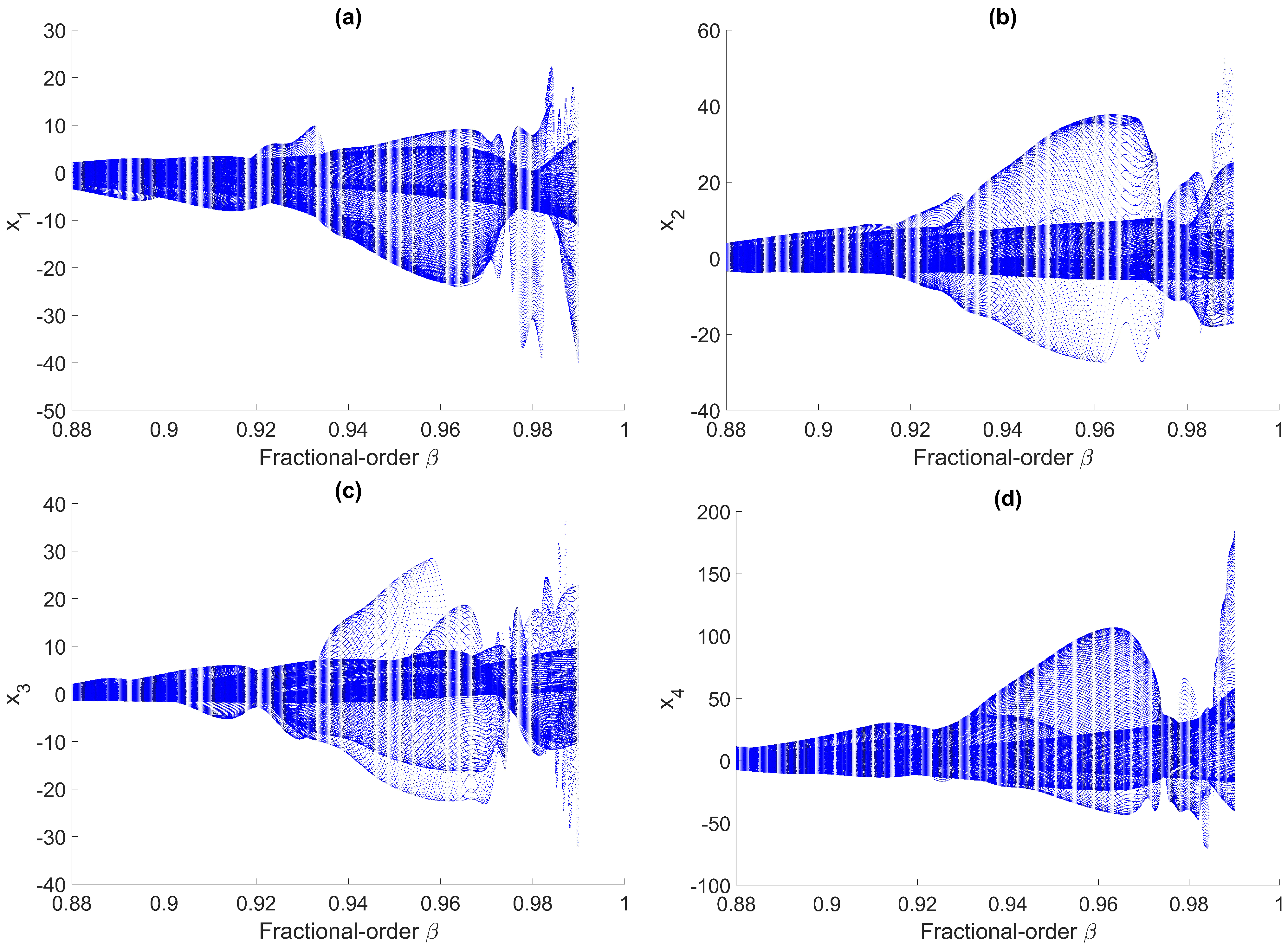
3.2. Bifurcation Analysis of the Proposed System

The bifurcation diagrams (see Figure 2) of state variable for parameter variations reveal intricate dynamical transitions and sensitivity across different ranges for each parameter:

• As ${\sigma }_2$ varies over $[50,70]$, the diagrams for (a) $x_1$, (b) $x_2$, and (c) $x_4$ showcase complex and chaotic behaviors, with evident bifurcation patterns indicating high sensitivity to changes in ${\sigma }_2$.
• For ${\sigma }_4$ within the range $[5,35]$, the diagrams of (d) $x_4$, (e) $x_5$, and (f) $x_7$ illustrate dynamic transitions and bifurcation phenomena, underscoring the parameter’s influence on system complexity and sensitivity.
• Varying ${\sigma }_6$ from 0 to 3 in subfigures (g) $x_1$, (h) $x_2$, and (i) $x_3$ further highlights hyperchaotic characteristics, with the diagrams demonstrating extensive transitions and sensitivity across the specified range.

Figure 2. Bifurcation diagrams of system variables with respect to varying parameters: (a) $x_1$, (b) $x_2$, (c) $x_4$ with respect to parameter ${\sigma }_2$, (d) $x_4$, (e) $x_5$, (f) $x_7$ with respect to parameter ${\sigma }_4$, (g) $x_1$, (h) $x_2$, (i) $x_3$ with respect to parameter ${\sigma }_6$.

Bifurcation diagrams (see Figure 3) of the fractional-order ($\beta$) for the system variables, illustrated in (a) $x_1$, (b) $x_2$, (c) $x_3$, and (d) $x_4$, reveal dynamic responses across the range $[0.88,0.99]$. These diagrams emphasize the impact of the FO $\beta$ on the hyperchaotic behavior of the system, showcasing intricate transitions and sensitivity to variations in $\beta$, which are crucial for understanding its role in the system’s complex dynamics.

Figure 3. Fractional-order ($\beta$) bifurcation diagrams for (a) $x_1$, (b) $x_2$, (c) $x_3$, (d) $x_4$.

The FO $\beta$ significantly influences the behavior of the 10D hyperchaotic system, as demonstrated in the bifurcation diagrams within the range $[0.88,0.99]$. This range provides a variety of options for $\beta$, allowing for flexible control over the system’s dynamics and complexity. Each incremental adjustment in $\beta$ introduces distinct dynamical patterns, serving as a powerful tool for modifying the system’s hyperchaotic characteristics.

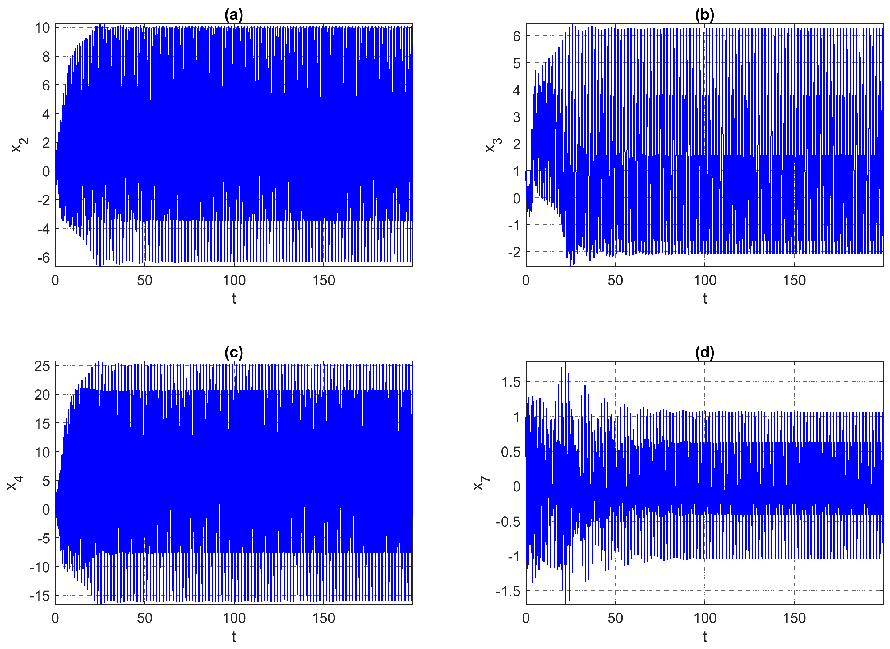
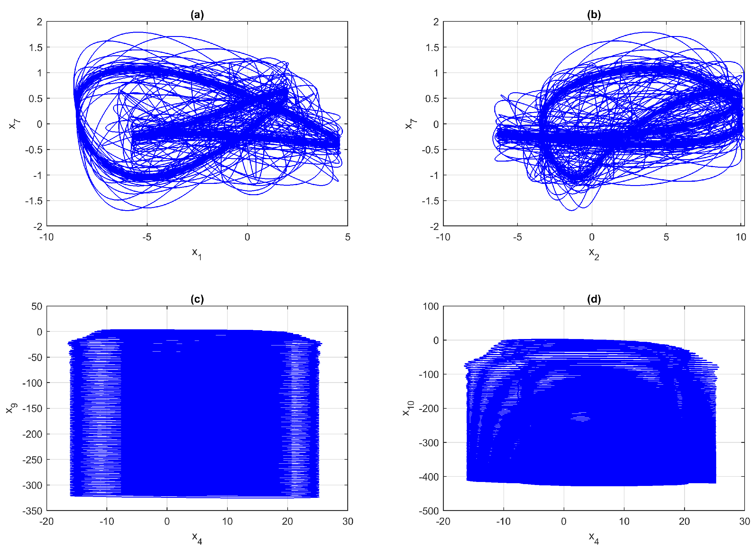
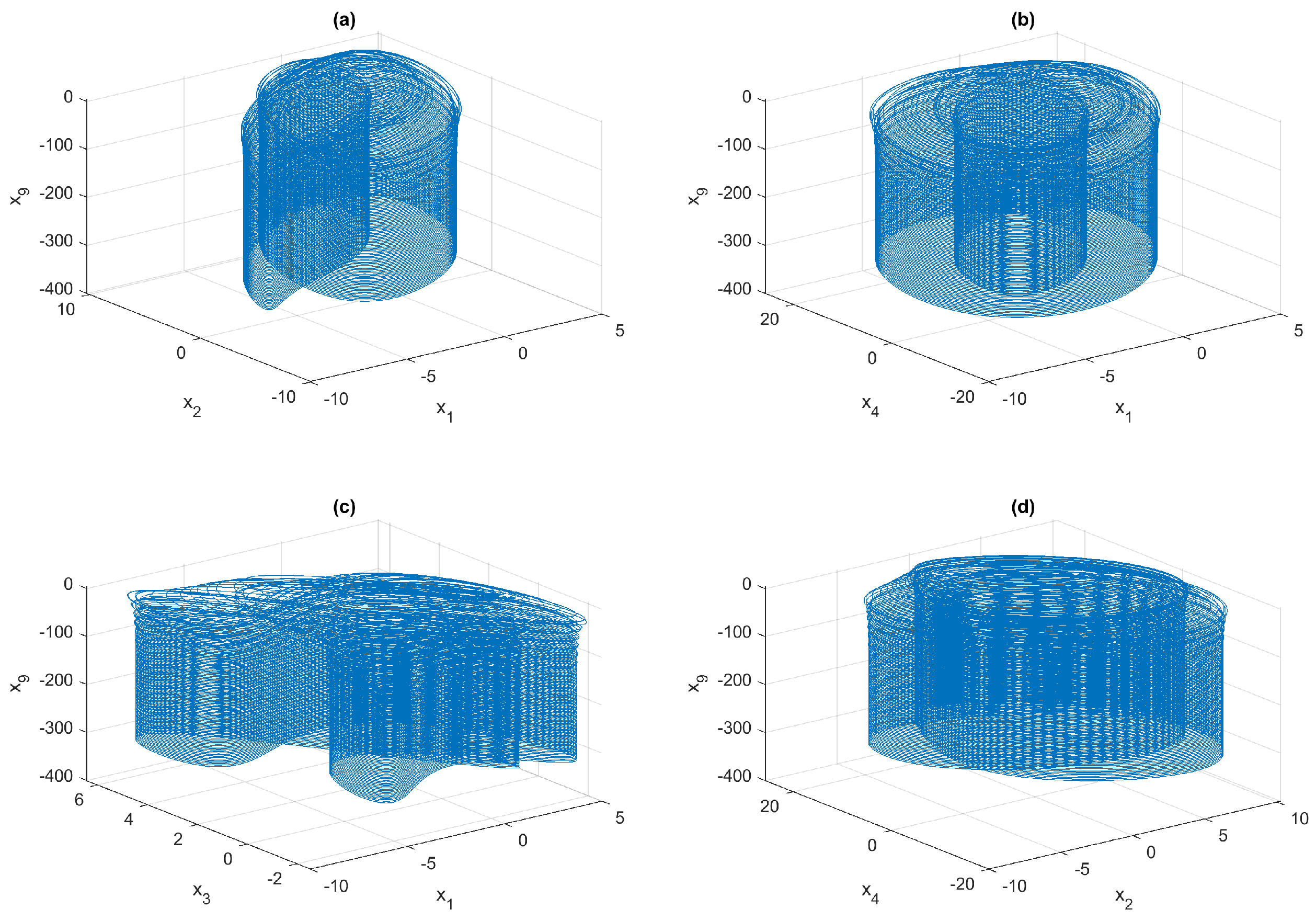
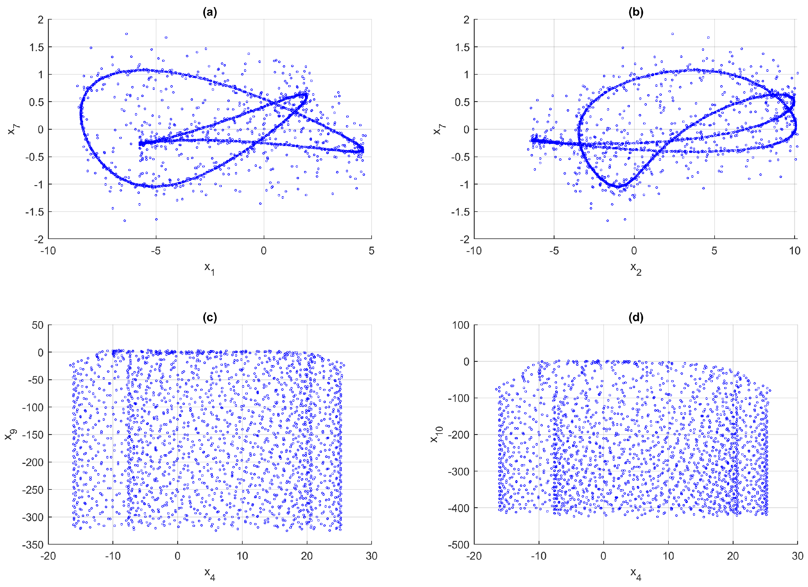
3.3. Phase Diagrams and Dynamical Trajectories

The time series analysis of the variables $x_2$, $x_3$, $x_4$, and $x_7$, displayed in subplots (a) to (d) in Figure 4, reveals the intricate behavior of a hyperchaotic system. In subplot (a), the variable $x_2$ exhibits irregular oscillations with a wide range of amplitudes, indicating chaotic dynamics devoid of periodicity. Similarly, subplot (b) shows that $x_3$ demonstrates high-frequency oscillations with smaller amplitudes over time, further illustrating the sensitive dependence on initial conditions that is characteristic of hyperchaotic systems. Subplots (c) and (d) present the time evolution of $x_4$ and $x_7$, respectively, both of which also exhibit complex, non-periodic behavior with a broader amplitude range, suggesting a stronger chaotic influence. Overall, the time series for all four variables underscores the hyperchaotic nature of the system, where multiple positive Lyapunov exponents propel the system into multi-dimensional chaotic trajectories, reflecting its highly unpredictable and complex behavior.

Figure 4. The chaotic time series analysis of 10D hyperchaotic FOS (2): (a) $x_2\left(t\right)$, (b) $x_3\left(t\right)$, (c) $x_4\left(t\right)$, (d) $x_7\left(t\right)$.

The time histories of the state variables $x_1\left(t\right)$, $x_2\left(t\right)$, $x_3\left(t\right)$, and $x_4\left(t\right)$ presented in Figure 5 reveal significant dynamic changes in the hyperchaotic system as the parameter ${\sigma }_1$ varies. At ${\sigma }_1=-1.4,0.4,1.4,2.4$, the amplitude and complexity of the oscillations intensify, indicating a transition to more chaotic behavior. These results highlight the system’s high sensitivity to parameter variations, which is characteristic of hyperchaotic dynamics.

Figure 5. Time histories of state variables (a) $x_1\left(t\right)$, (b) $x_2\left(t\right)$, (c) $x_3\left(t\right)$, (d) $x_4\left(t\right)$ for different values of parameter ${\sigma }_1=-1.4,0.4,1.4,2.4$.

The sensitivity analysis depicted in the time histories of variables (a) $x_3\left(t\right)$, (b) $x_5\left(t\right)$, (c) $x_7\left(t\right)$, (d) $x_8\left(t\right)$, as presented in Figure 6 under two different initial conditions demonstrates the hyperchaotic system’s response to initial conditions. Distinct trajectories arise from initial conditions.

Figure 6. Time histories for sensitivity analysis of system variables (a) $x_3\left(t\right)$, (b) $x_5\left(t\right)$, (c) $x_7\left(t\right)$, (d) $x_8\left(t\right)$ under two different initial conditions.

$\mathrm{Set}1=(-1,0,1,4,1,5,1,1,1,-1)$ and $\mathrm{Set}2=(0,-0.5,-0.5,-0.5,-1.0,3.0,0.5,-0.5,$$1.0,0.5)$, revealing the system’s extreme sensitivity to small variations in initial conditions, which is a characteristic of hyperchaotic dynamics.

In comparison to earlier works, including those by Tian [21] and Yu [34], the findings of this study reveal a significantly enhanced hyperchaotic behavior. Figure 7 indicates that:

Figure 7. The 2D phase trajectories of proposed hyperchaotic FOS (2): (a) $x_1–x_7$ phase diagram, (b) $x_2–x_7$ phase diagram, (c) $x_4–x_9$ phase diagram, (d) $x_4–x_{10}$ phase diagram.

The 2D phase trajectories of the proposed hyperchaotic FOS (2) are more effective at capturing the intricate complexity and richness of the system’s dynamics, providing a deeper and more accurate representation of its chaotic nature.

The 3D phase trajectories of the proposed hyperchaotic system, as illustrated in subplots (a) to (d) of Figure 8, exhibit the intricate folding and stretching patterns that are characteristic of hyperchaotic systems. These dynamic features underscore the presence of multiple attractors, where chaotic flows dominate the phase space. Subplot (a) presents the $x_1-x_2-x_9$ phase diagram, while subplot (b) displays the $x_1-x_4-x_9$ phase diagram, both revealing highly complex and overlapping trajectories. Subplots (c) and (d), which represent the $x_1-x_3-x_9$ and $x_2-x_4-x_9$ phase diagrams, further illustrate the system’s sensitivity to initial conditions, showcasing continuous stretching and folding behaviors that highlight the high-dimensional complexity of the hyperchaotic system.

Figure 8. The 3D phase trajectories of proposed hyperchaotic FOS (2): (a) $x_1-x_2-x_9$ phase diagram, (b) $x_1-x_4-x_9$ phase diagram, (c) $x_1-x_3-x_9$ phase diagram, (d) $x_2-x_4-x_9$ phase diagram.

The attractors exhibited by this system reveal a greater degree of complexity, unpredictability, and sensitivity compared to the results reported by H. Tian [21] for the 4D conditional symmetric FOS. Also, the obtained results demonstrate that the chaotic attractors generated by the proposed system are superior to those reported in previous studies, including [35,36,37], and the work by T. Lu [38], as clearly evidenced by the simulation results demonstrated in Figure 8.

The 2D Poincaré sections (Figure 9) reveal regions densely populated with points that form intricate, fractal-like structures. This pattern suggests that the system undergoes continuous bifurcation, indicative of the complex and chaotic behavior inherent in the dynamics of the attractor. The 3D Poincaré sections (Figure 10) further emphasize these characteristics, showcasing a clear presence of dense point distributions and fractal formations throughout the phase space. Collectively, these observations demonstrate the multiscroll nature of the system’s dynamics, highlighting its hyperchaotic behavior and the richness of its underlying structure.

Figure 9. The 2D Poincaré section of the hyperchaotic FOS (2): (a) $x_1-x_7$, (b) $x_2-x_7$, (c) $x_4-x_9$, and (d) $x_4-x_{10}$.

Figure 10. The 3D Poincaré section of the hyperchaotic FOS (2): (a) $x_1-x_2-x_9$, (b) $x_1-x_4-x_9$, (c) $x_1-x_3-x_9$, (d) $x_2-x_4-x_9$.

4. Complexity and Chaotic Properties of the Proposed FOS

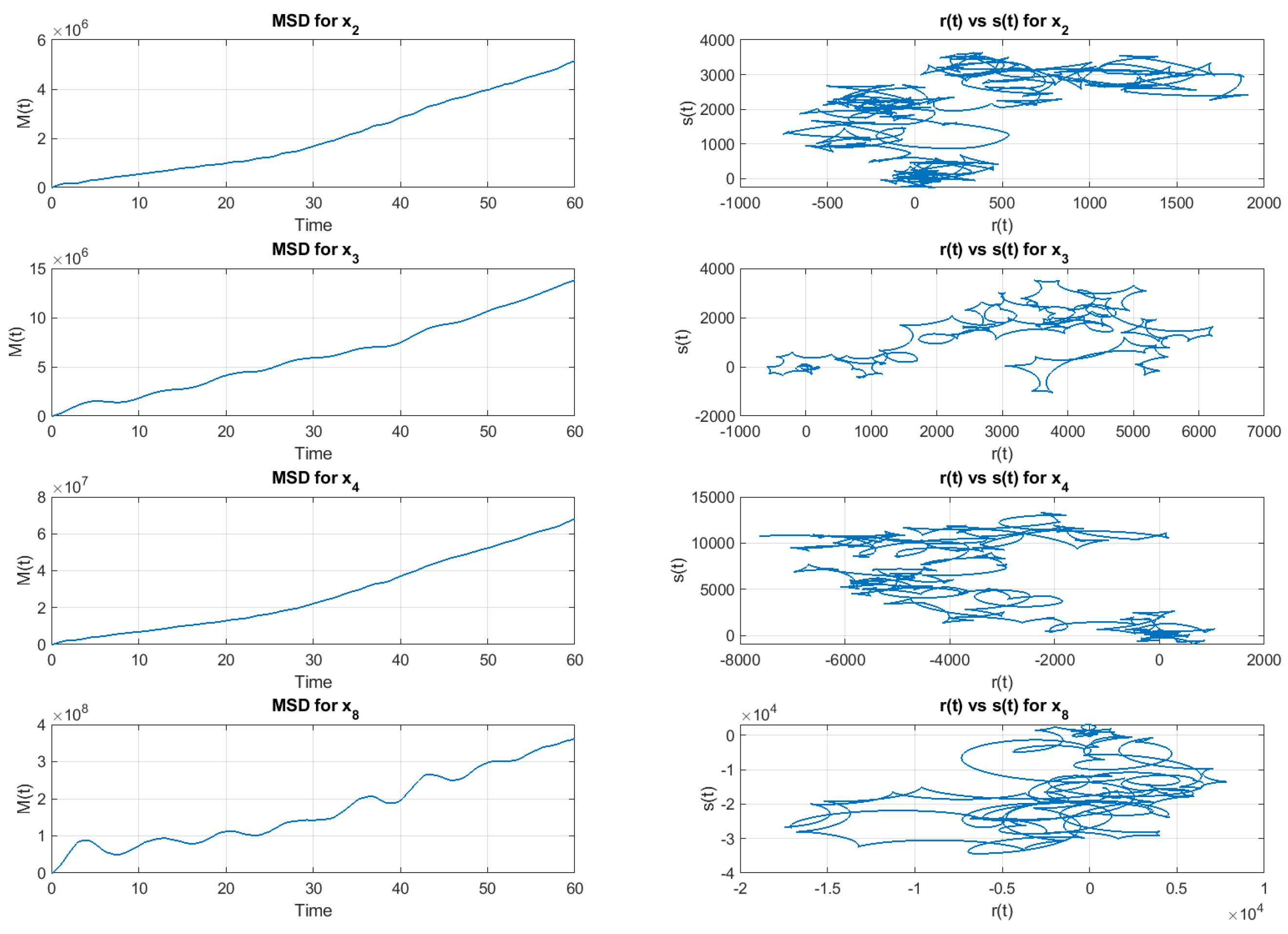
4.1. Analysis of 0-1 Test for Chaos

In 2004, Gottwald and Melbourne [39] introduced a novel approach known as the 0-1 test for chaos, which determines whether a deterministic dynamical system exhibits chaotic or non-chaotic behavior. Unlike traditional methods that rely on calculating the maximal Lyapunov exponent, this test operates directly on time-series data, thereby eliminating the need for phase-space reconstruction. Additionally, it is independent of the system’s dimensionality and the specific form of its governing equations. The method takes time-series data as input and produces an output of 0 or 1, indicating non-chaotic or chaotic dynamics, respectively. This test is broadly applicable to any deterministic dynamical system, including those governed by ordinary or partial differential equations and discrete maps.

We utilized the ‘0-1 test’ to confirm the presence of chaotic behavior in the numerical time series data. This test is a straightforward and effective method used to determine whether a dynamical system exhibits chaotic behavior. This test is based on analyzing the trajectory of the system in phase space and quantifying its behavior using a binary classification (0 for regular dynamics and 1 for chaos) [40,41]. Its simplicity and reliability have made it a popular tool in chaos theory, especially for experimental and computational data. In this study, we applied the 0-1 test to evaluate the behavior of the proposed 10D FOS (2).

One of the primary advantages of this test is its ability to provide an intuitive visualization of the dynamical system within the translational variables $(r-s)$ space. For the designed 10D ODE system (2), which consists of the state variables $x_1,x_2,\dots ,x_{10}$, the translational variables $r\left(t\right)$ and $s\left(t\right)$ are defined using a fixed phase value $\alpha$ as follows:

$$\begin{array}{cc}\hfill r_{\mu }\left(t\right)& =\sum _{l=1}^t{x}_{\mu }\left(l\right)cos\left(l\alpha \right),\hfill \\ \hfill s_{\mu }\left(t\right)& =\sum _{l=1}^t{x}_{\mu }\left(l\right)sin\left(l\alpha \right).\hfill \end{array}$$

(17)

Equation (17) describes the translation variables $r_{\mu }\left(t\right)$ and $s_{\mu }\left(t\right)$ associated with every variable $x_{\mu }\left(t\right)$ in the designed 10D system (2). These translation variables provide insights into the dynamics of the system within a transformed coordinate framework, which is defined using trigonometric functions with a constant phase parameter $\alpha$. MSD is a crucial metric for evaluating the system’s diffusive properties over time, offering insights into the extent to which the state variables $x_{\mu }\left(t\right)$ disperse within the phase space as time progresses.

For a given particle $\mu$, the displacement in the $x_{\mu }$-direction between two time steps, denoted by l and $l+n$, can be expressed as $r_{\mu }(l+n)-r_{\mu }\left(l\right)$. In the same way, if applicable, the displacement in the $y_{\mu }$-direction is represented by $s_{\mu }(l+n)-s_{\mu }\left(l\right)$.

The squared displacement along both the $x_{\mu }$-axis and $y_{\mu }$-axis can be expressed mathematically as follows:

$${(r_{\mu }(l+n)-r_{\mu }\left(l\right))}^2+{(s_{\mu }(l+n)-s_{\mu }\left(l\right))}^2.$$

This equation defines the squared Euclidean distance covered by a particle as it moves within a two-dimensional plane, assuming that $r_{\mu }$ and $s_{\mu }$ correspond to the $x_{\mu }$ and $y_{\mu }$ coordinates, respectively. The use of the squared Euclidean distance allows for an effective quantification of the particle’s spatial displacement, which is particularly useful in understanding its diffusive behavior in the system.

MSD, which is represented by $M_{\mu }\left(n\right)$, is determined by calculating the average of the squared differences in displacements for all possible time intervals l corresponding to a specific time lag n as follows:

$$\begin{array}{c}\hfill \mathrm{MSD}=M_{\mu }\left(n\right)={\displaystyle \frac{1}{N}}\sum _{l=1}^N\left[{(r_{\mu }(l+n)-r_{\mu }\left(l\right))}^2+{(s_{\mu }(l+n)-s_{\mu }\left(l\right))}^2\right],\end{array}$$

(18)

where the variables $s_{\mu }\left(t\right)$ and $r_{\mu }\left(t\right)$ correspond to the translational components obtained by projecting the time series of the dynamical system onto two orthogonal directions determined by a randomly selected angle. The term $x_{\mu }\left(l\right)$ indicates the value of the $\mu$-th state variable at a specific time step l. The parameter $N=⌊{\displaystyle \frac{n_{\mathrm{vals}}}{2}}⌋$ defines the total number of data points in the time series and serves as the maximum limit for summation. Here, $n_{\mathrm{vals}}$ represents the total number of discrete time points in the series, ranging from $x_1$ to $x_{10}$. Finally, $M_{\mu }\left(n\right)$ denotes the MSD of points in the $(r,s)$ plane for a given time lag n.

In the context of the 0-1 test for chaos, a system is identified as regular if the metric $M_{\mu }\left(n\right)$ grows sub-linearly or stays bounded as n increases. On the other hand, if $M_{\mu }\left(n\right)$ grows linearly with n, the system is considered chaotic (refer to [40,41]). In this analysis, we employed a fixed phase parameter $\alpha ={\displaystyle \frac{\pi }{4}}$.

The 0-1 test for chaos was utilized to analyze the time series data of the state variables $x_1,x_2,\dots ,x_{10}$ derived from the 10-dimensional ordinary differential equation (ODE) system. The results corresponding to the state variables $x_2,x_3,x_4$, and $x_8$ are illustrated in Figure 11.

Figure 11. The 0-1 test for chaos: numerical time series of mean square displacement $\left[M_{\mu }\left(n\right)\right]$, and dynamics of translation components $[r_{\mu }\left(t\right),s_{\mu }\left(t\right)]$ for $x_2$, $x_3$, $x_4$, and $x_8$.

Subsequently, the diffusion characteristics of $r_{\mu }\left(t\right)$ and $s_{\mu }\left(t\right)$ are examined to determine the mean squared displacement $\left[M_{\mu }\left(n\right)\right]$. Based on the theoretical principles, a linear growth in $\left[M_{\mu }\left(n\right)\right]$ with respect to time signifies chaotic dynamics, as illustrated in Figure 11.

The MSD plots clearly demonstrate a linear progression over time, signifying the presence of chaotic behavior. This consistent linear trend in the MSD indicates exponential divergence of the system’s trajectories, a defining characteristic of chaos. The plots of $[r_{\mu }\left(t\right),s_{\mu }\left(t\right)]$ demonstrate a disordered, irregular, and non-repeating structure, as illustrated in Figure 11. This characteristic emphasizes the chaotic dynamics of the translational components $[r_{\mu }\left(t\right),s_{\mu }\left(t\right)]$. The apparent randomness in these plots further underscores the lack of periodicity and predictability, consistent with the fundamental properties of chaotic systems.

The parameter K in the 0-1 test for chaos is a statistical measure used to identify whether a dynamical system exhibits chaotic behavior. It is defined as

$$K=\underset{n\to \infty }{lim}{\displaystyle \frac{ln\left({\mathrm{M}}_{\mu }\left(n\right)\right)}{ln\left(n\right)}}.$$

If $K\approx 1$, then the system exhibits chaotic behavior as the MSD grows diffusively, and when $K\approx 0$, the system is non-chaotic, indicating bounded or regular dynamics.

The 0-1 test statistic K values for the variables $x_2,x_3,x_4$ and $x_8$ are calculated using MATLAB R2023b to analyze the FOS (2) and presented in Table 3.

Table 3. Numerical analysis of statistic K values for the variables $x_2,x_3,x_4$, and $x_8$.

${\mathit{K}}_{{\mathit{x}}_2}$	${\mathit{K}}_{{\mathit{x}}_3}$	${\mathit{K}}_{{\mathit{x}}_4}$	${\mathit{K}}_{{\mathit{x}}_8}$
1.056830	1.160566	1.123059	0.819398

From Table 3, it is observed that $K_{x_2}$, $K_{x_3}$, and $K_{x_4}$ exhibit K-values exceeding 1, indicating hyperchaotic behavior. These values signify the presence of highly intricate dynamics characterized by at least two positive Lyapunov exponents, a defining feature of hyperchaotic systems. In contrast, the statistic K-value associated with $K_{x_8}$, which lies below 1 but above 0.8, suggests standard chaotic behavior. These findings highlight the distinction in the dynamical regimes.

4.2. LEs and Kaplan–Yorke Dimension

Based on chaos theory, a higher Kaplan–Yorke dimension signifies increased complexity in the behavior of dynamical systems [42]. The Kaplan–Yorke dimension presents a quantitative measure of the chaotic dynamics by estimating the effective number of degrees of freedom in the system, offering deeper insights into its complexity. For the fractional-order system (FOS) described in (2), the Kaplan–Yorke dimension $D_{KY}$ is calculated as follows:

$$D_{KY}=\nu +{\displaystyle \frac{{\sum }_{\mu =1}^{\nu }{\lambda }_{\mu }}{|{\lambda }_{\nu +1}|}},$$

where $\nu$ represents the greatest integer value, defined as

$$\sum _{\mu =1}^{\nu }{\lambda }_{\mu }>0\mathrm{and}\sum _{\mu =1}^{\nu +1}{\lambda }_{\mu }<0.$$

For a system of 10 fractional orders, denoted as $\mathcal{O}$, and with parameters ${\sigma }_1=-2.6$ and ${\sigma }_9=2.9$, the Kaplan–Yorke dimension, represented by $D_{KY}$, can be determined using the provided Lyapunov exponents (see Table 1) and following the steps outlined in Algorithm 3,

$$2.5259,1.3293,0.5877,0.5842,0.5741,0.4566,0.2624,-0.0705,-0.6268,-8.1137$$

Then, $D_{KY}$ can be calculated as follows:

$$D_{KY}=9+{\displaystyle \frac{{\sum }_{\mu =1}^9{\lambda }_{\mu }}{|{\lambda }_{10}|}}=9+{\displaystyle \frac{6.2775}{8.1137}}=9.693,$$

where $\nu =9$ is the largest integer such that

$$\sum _{\mu =1}^9{\lambda }_{\mu }=6.2775>0\mathrm{and}\sum _{\mu =1}^{10}{\lambda }_{\mu }=-1.8362<0.$$

Table 4 presents a comparative analysis of the fractional dimensions of the newly proposed fractional-order (FO) system (2) and several well-known hyperchaotic systems reported in the literature.

Algorithm 3 Compute Kaplan–Yorke dimension ($D_{KY}$) using MATLAB

Require:  $LE$: Vector of LEs Ensure:  $D_{KY}$: The Kaplan–Yorke Dimension  1: Sort $LE$ in descending order: $LE\_sorted\leftarrow \mathrm{sort}(LE,‘\mathrm{descend}’)$  2: Initialize $cumulative\_sum\leftarrow 0$, $index\leftarrow 0$  3: for $i\leftarrow 1$ to $\mathrm{length}(LE\_sorted)$ do  4:     $cumulative\_sum\leftarrow cumulative\_sum+LE\_sorted\left[i\right]$  5:     if $cumulative\_sum<0$ then  6:         $index\leftarrow i-1$  7:         Break  8:     end if  9: end for 10: if  $index==0$  then 11:     $D_{KY}\leftarrow \mathrm{NaN}$                                    ▹ Undefined if no positive cumulative sum exists 12: else 13:     $D_{KY}\leftarrow index+{\displaystyle \frac{{\sum }_{j=1}^{index}LE\_sorted\left[j\right]}{|LE\_sorted[index+1\left]\right|}}$ 14: end if 15: Output: $D_{KY}$f

Table 4. Comparative analysis of Kaplan–Yorke fractal dimension with various well-known hyperchaotic systems from the literature.

ODE Systems	Fractal Dimensions
Proposed 10D system for ${\sigma }_9=91$	8.164
Proposed 10D system for ${\sigma }_1=-2.6,{\sigma }_9=2.9$	9.693
Proposed 10D system for ${\sigma }_9=5.8$	9.369
7D system proposed by Hu and Chan [43]	6.732
7D system introduced by Yang [44]	6.149
7D system developed by Yu et al. [45]	5.278
7D system described by Lagmiri et al. [46]	2.091
7D system presented by Varan and Akgul [47]	2.175
8D system constructed by Biban et al. [48]	7.13
9D system outlined by Mahmoud et al. [35]	5.128
9D system reported by Zhu et al. [36]	2.171
10D system established by Jianliang et al. [37]	2.429

The Kaplan–Yorke dimension is a widely recognized metric used to assess the complexity of chaotic attractors, providing an estimate of the fractal structure and the degree of unpredictability of a given system. Table 4 compares the Kaplan–Yorke dimensions of the proposed 10-dimensional fractional-order system (10D FOS) with those of existing systems reported in the literature. The proposed system demonstrates significant improvements in terms of Kaplan–Yorke dimension, ranging from 8.164 to 9.693, depending on the selected parameters. This indicates a higher level of complexity and chaotic behavior compared to other systems, such as the 7D Hu and Chan system ($6.732$), the 8D Biban system ($7.13$), and the 9D Mahmoud system ($5.128$). Specifically, for ${\sigma }_1=-2.6$ and ${\sigma }_9=2.9$, the proposed system achieves a fractal dimension of $9.693$, which is considerably higher than that of the other systems compared. The elevated Kaplan–Yorke dimension signifies enhanced chaotic properties, leading to more unpredictable and complex behaviors, which are crucial for applications such as secure communication and encryption, where high-dimensional chaotic behavior is desirable.

The Kaplan–Yorke fractal dimensions outlined in Table 4 reveal that the calculated values of $D_{KY}$ are notably higher than those observed in other dynamical systems. This indicates that the proposed 10D fractional-order system (FOS) in (2) exhibits highly intricate hyperchaotic behavior.

4.3. Kolmogorov–Sinai (KS) Entropy

The Kolmogorov–Sinai (KS) entropy, also referred to as metric entropy, represents the rate at which information is generated in a dynamical system. Kolmogorov–Sinai (KS) entropy [49] quantifies the complexity and unpredictability of a dynamical system by measuring the average rate of information production. It is defined as

$$E_{\mathrm{KS}}=\underset{\mathcal{P}}{sup}\underset{n\to \infty }{lim}{\displaystyle \frac{1}{n}}H\left(\underset{i=0}{\overset{n-1}{\bigvee }}{T}^{-i}\mathcal{P}\right),$$

(19)

where $\mathcal{P}$ is a measurable partition of the system’s phase space, T is the dynamical evolution operator (e.g., a map or flow), $H(·)$ represents the Shannon entropy of the partition, and ${\bigvee }_{i=0}^{n-1}{T}^{-i}\mathcal{P}$ is the joint refinement of the partition under the evolution of the system over n steps.

For systems with positive Lyapunov exponents ${\lambda }_1,{\lambda }_2,\dots ,{\lambda }_k$, the KS entropy is related to the sum of these exponents by Pesin’s theorem [50],

$$E_{\mathrm{KS}}=\sum _{i=1}^k{\lambda }_i,{\lambda }_i>0,$$

(20)

where ${\lambda }_i$ are the positive Lyapunov exponents of the system.

The values of KS entropy present the degree of chaos present in each parameter set of the proposed FOS. Higher KS entropy values correspond to higher complexity and more chaotic dynamics. Observing the positive Lyapunov exponents (LEs) from Table 1, the parameter set with ${\sigma }_1=-2.6$ and ${\sigma }_9=2.9$ exhibits the highest KS entropy of 6.32. This suggests a greater degree of exponential divergence of nearby trajectories, indicating a highly chaotic system. Such a high value implies that the system’s dynamics are extremely sensitive to initial conditions, resulting in rapid divergence and significant unpredictability.

The calculated results for the KS entropy across the various parameter sets indicate more pronounced levels of complexity and chaos compared to the results presented by Mahmoud [35], Zhu [36], Jianliang [37], Biban [48], and Benkouider [51]. These experimental outcomes suggest that the proposed FOS (2) exhibits superior chaotic characteristics, surpassing those documented in previous studies.

4.4. Analysis of Perron Effect

Analysis of the Perron effect describes a situation in which one Lyapunov exponent (LE) predominantly influences the dynamics of a system, effectively causing a single direction in phase space to dictate the overall behavior of the system. This phenomenon is mathematically evident when the largest LE (LLE) is extensively greater than the others, represented as ${\lambda }_1\gg {\lambda }_2\ge {\lambda }_3\ge \cdots \ge {\lambda }_{10}$. When the dominant Lyapunov exponent, ${\lambda }_1$, greatly exceeds the remaining exponents, it indicates a strong Perron effect, suggesting that the system’s dynamics are primarily governed by this leading direction.

The manifestation of the Perron effect is clearly observed in the Largest Lyapunov Exponents (LLEs) for the fractional-order system (FOS) presented in Table 1. The results reveal the Lyapunov Exponents (LEs) corresponding to ten distinct fractional-orders, denoted as $\mathcal{O}$. Notably, the LLEs (${\lambda }_1$) are significantly positive, indicating a strong exponential divergence of nearby trajectories. The consistently dominant LLEs across three parameter values of ${\sigma }_1=-2.6$, and ${\sigma }_9$ (91, 2.9, 5.8) affirm the presence of hyperchaotic behavior, in accordance with the Perron effect. This reinforces the system’s sensitivity to initial conditions and its complex dynamical properties.

Upon examining the largest Lyapunov exponents (LLEs) of the 10D hyperchaotic system, as presented in Table 1, the pronounced dominance of ${\lambda }_1$ (with values of 1.17, 2.53, and 1.44) over the other exponents indicates a significant directional influence within the phase space. This observation closely aligns with the findings of Mahmoud [35], Zhu [36], Jianliang [37], Biban [48], and Benkouider [51] further reinforcing the validity of the results through the well-known Perron effect, which characterizes the behavior of the system in high-dimensional chaotic dynamics.

5. Quantitative Comparison and Complexity Analysis

5.1. Error Margins

To ensure statistical rigor, we compare the Lyapunov spectrum and Kolmogorov–Sinai (KS) entropy of the proposed 10-dimensional fractional-order system (10D FOS) with those of existing hyperchaotic systems, focusing on the error margins in their numerical computation as presented in Table 5. This comparison highlights the stability and accuracy of the proposed system.

Table 5. Comparison of Lyapunov exponents and error margins.

System	Positive LEs	Negative LEs	Error Margin (LE)	KS Entropy	Error Margin (KS)
Proposed 10D FOS	$2.53,1.33,0.59$	$-0.07,-0.63,-8.11$	$\pm 0.01$	$4.45$	$\pm 0.02$
Chen’s System [8]	$1.18,0.42$	$-0.24,-1.02$	$\pm 0.05$	$1.60$	$\pm 0.05$
Rössler’s System [52]	$0.98,0.12$	$-0.36,-0.98$	$\pm 0.05$	$1.10$	$\pm 0.05$
Lorenz’s System [1]	$0.91,0.03$	$-0.64,-1.34$	$\pm 0.07$	$0.91$	$\pm 0.06$

The proposed system achieves a significantly lower error margin ($\pm 0.01$) compared to existing systems such as the Chen ($\pm 0.05$) and Rössler ($\pm 0.05$) hyperchaotic systems. This indicates higher numerical stability and precision in LE computation. The KS entropy for the proposed system ($4.45\pm 0.02$) demonstrates both higher complexity and reduced computational uncertainty compared to existing systems. For example, the Chen system exhibits a KS entropy of $1.60\pm 0.05$, reflecting lower complexity and higher variability.

The error margins for the proposed system remain consistently small across all metrics, suggesting enhanced numerical robustness due to the designed computational approach (e.g., Grünwald–Letnikov fractional derivative method and Gram–Schmidt Reorthonormalization). The proposed hyperchaotic system demonstrates superior accuracy and precision in computing Lyapunov exponents and KS entropy compared to existing hyperchaotic systems. The reduced error margins highlight its enhanced numerical stability, making it a reliable for applications requiring precise chaotic dynamics.

5.2. Computational Complexity

The proposed method exhibits a complexity of $\mathcal{O}(N·M·d^2)$, where N represents the number of time steps, M denotes the number of iterations for Gram–Schmidt orthonormalization, and $d=10$ corresponds to the system’s dimensionality. Compared to existing methods, the proposed technique achieves higher efficiency due to its focus on memory principles and orthonormalization. When we analyze the comparison results presented in Table 6, then we can see that the memory usage of $\mathcal{O}\left(d^2\right)$ is significantly lower than methods requiring higher-order computations such as $\mathcal{O}\left(d^3\right)$, making the proposed method more suitable for high-dimensional systems. The execution time for the proposed method, 200 s, is lower than other methods, demonstrating its computational efficiency.

Table 6. Quantitative comparison of computational complexity.

Method	Order of Complexity	Memory Requirements	Execution Time (s)
Proposed 10D FOS (G-L + GSR)	$\mathcal{O}(N·M·d^2)$	$\mathcal{O}\left(d^2\right)$	200
Caputo-Based Predictor–Corrector [53]	$\mathcal{O}(N·d^3)$	$\mathcal{O}\left(d^3\right)$	450
Caputo-Based Predictor–Corrector [54]	$\mathcal{O}(N·d^3)$	$\mathcal{O}\left(d^3\right)$	450
Mittag–Leffler Approximation [16]	$\mathcal{O}(N^2·d^3)$	$\mathcal{O}\left(d^3\right)$	500

The integration of the Grünwald–Letnikov operator with Gram–Schmidt Reorthonormalization (GSR) significantly reduces computational overhead, maintaining numerical accuracy while minimizing execution time. Compared to traditional methods such as the Caputo-based predictor-corrector and Mittag–Leffler approximation, the proposed approach achieves a balance between accuracy and efficiency, making it suitable for real-time simulations of high-dimensional fractional-order systems.

5.3. Implementation Challenges and Computational Overhead

The proposed 10D fractional-order system (FOS) and its method for computing the Lyapunov exponent (LE) offer valuable insights into the dynamics of hyperchaotic systems. However, implementing this algorithm presents practical challenges that must be addressed to ensure both efficiency and feasibility.

A key challenge is the significant computational overhead associated with the Grünwald–Letnikov (G-L) method, which serves as the foundation of the algorithm. This method heavily relies on historical data to compute fractional derivatives, resulting in substantial memory requirements. Each variable’s memory allocation must accommodate data from all previous time steps. Furthermore, the iterative calculation of binomial coefficients adds to the computational complexity. The Gram–Schmidt Reorthonormalization process, which is essential for mitigating numerical instabilities caused by positive Lyapunov exponents, further exacerbates these demands. For example, running the algorithm on a system equipped with an Intel i7-10700 CPU (Intel Corporation, Beijing, China) and 16 GB of RAM required approximately 150 s for a simulation with $t=200$ and $h=0.001$. Increasing the simulation duration or decreasing the time step significantly extends execution times.

Another critical factor is hardware feasibility. While personal computers can manage the computations, they are susceptible to prolonged execution times and potential memory allocation issues during extended simulations or when using smaller time steps. High-performance computing systems, such as GPUs or parallel computing frameworks like CUDA, provide a practical solution by leveraging task parallelization to significantly reduce execution times. However, implementing the algorithm on resource-limited embedded systems remains impractical due to the substantial memory and processing requirements of the 10D FOS.

Scalability also poses a significant challenge. Extending the algorithm to higher-dimensional systems or systems with additional fractional orders results in an exponential increase in computational demands, with complexity growing as $\mathcal{O}(N·M·d^2)$, where d represents the system’s dimension. Parallelizing computations, such as memory term summations and Jacobian matrix calculations, can enhance scalability; however, it necessitates careful synchronization to ensure numerical accuracy.

Several optimizations have been proposed to address these challenges. Implementing a sliding memory window can reduce memory requirements by limiting the historical data utilized in computations. Parallelizing tasks across multicore CPUs or GPUs can enhance efficiency. Additionally, adopting sparse matrix representations for the Jacobian and deviation matrices can decrease both memory usage and computational time. Dynamic time-stepping, which replaces the fixed step size h with an adaptively adjusted step size, can effectively balance computational accuracy and execution time. These enhancements can render the algorithm more viable for practical applications, even in resource-constrained environments.

6. Results and Discussions

The numerical analysis of the proposed 10D fractional-order system (FOS) offers significant insights into its intricate dynamical behavior. Utilizing the fractional-order Chen system and integrating the memory effect via the Grünwald–Letnikov (G-L) derivative, the system exhibits complex hyperchaotic dynamics. This is demonstrated by the presence of multiple positive Lyapunov exponents (LEs), which highlight the system’s extreme sensitivity to initial conditions and confirm its high-dimensional chaotic characteristics. These results underscore the effectiveness of fractional-order derivatives in capturing the memory effect, which is pivotal in generating the observed hyperchaotic behavior.

The analysis of phase portraits and time series under different parameter settings strongly supports the presence of chaotic dynamics in the system. Bifurcation analyses of both state variables and fractional-orders demonstrate the hyperchaotic characteristics of the proposed model. The 2D and 3D phase plots demonstrate intricate and tightly packed trajectories, emphasizing the system’s high sensitivity to initial conditions and the intricate interplay between its state variables. These findings align with earlier research while highlighting a greater degree of complexity and chaotic behavior, which can be attributed to the effects of fractional differentiation. Furthermore, the Kaplan–Yorke dimension provides additional support for these results by demonstrating that the designed system exhibits a greater fractal dimension compared to other known hyperchaotic systems.

Furthermore, the system’s stability and chaotic behavior are thoroughly examined through the Perron effect, Kolmogorov–Sinai (KS) entropy, the Kaplan–Yorke dimension, and the 0-1 test for chaos. The findings reveal that the Kaplan–Yorke dimension of the designed system is considerably higher, highlighting increased complexity and more intense chaotic dynamics compared to the results presented in [35,36,37,43,44,45,46,47,48].

The analysis of the KS entropy and Perron effect values reveals a significant increase in the system’s information production rate and unpredictability, surpassing the numerical outcomes reported in [35,36,37,48,51]. Numerical and simulation results collectively demonstrate the efficiency of the designed mathematical approach in accurately capturing the intricate behavior of hyperchaotic FOS. This establishes a reliable framework for exploring the dynamics of complex systems governed by fractional-order derivatives.

7. Summary of Results

This study introduces a novel 10-dimensional fractional-order chaotic system that leverages the memory effect of the Grünwald–Letnikov (G-L) derivative to exhibit hyperchaotic behavior. The dynamical properties of the proposed system are thoroughly analyzed using Lyapunov exponents (LEs) and bifurcation analysis, considering the influence of both state variables and fractional orders. While several established methods exist for calculating LEs in integer-order systems, these approaches are insufficient for fractional-order systems (FOS) due to the non-local characteristics intrinsic to fractional derivatives.

To evaluate the hyperchaotic nature of the proposed model, sensitivity analyses were performed by examining variations in state variables under two different initial conditions, as well as time histories for various parameter values. Comparative assessments with existing hyperchaotic systems demonstrate the improved accuracy and complexity of the proposed model, supported by advanced metrics such as the Kaplan–Yorke dimension, KS entropy, the Perron effect, and the 0-1 chaos test. Overall, these findings confirm that the proposed system provides a robust and precise framework for investigating high-dimensional fractional-order chaos, significantly enhancing both theoretical and practical insights into fractional-order dynamics.

8. Future Recommendations and Applications

The proposed 10-dimensional fractional-order system (FOS) exhibits hyperchaotic dynamics with a high-dimensional structure, presenting substantial potential for the development of advanced cryptographic techniques. Its intricate and high-dimensional behavior, characterized by multiple positive Lyapunov exponents (LEs) and a significant Kaplan–Yorke dimension, ensures the generation of highly complex and unpredictable signals. These signals are particularly well-suited for the generation of cryptographic keys, offering robust resistance against various types of attacks. Consequently, the proposed system enhances the security of encryption algorithms and bolsters their resilience in cryptographic applications.

Additionally, the proposed 10-dimensional and higher-dimensional hyperchaotic systems provide significant applications in image encryption, especially when combined with the Fibonacci $2\times 2$-matrix to enhance confusion during the encryption process. This method effectively addresses the limitations of small key spaces typically associated with image encryption algorithms that depend on low-dimensional chaotic maps, thereby considerably improving security and robustness.

Furthermore, these findings provide valuable insights for the design of chaotic circuits based on the 10-dimensional hyperchaotic system, facilitating practical implementations in real-world cryptographic and signal processing applications.

References

- Lorenz, E.N. Deterministic nonperiodic flow. J. Atmos. Sci. 1963, 20, 130–141. [Google Scholar] [CrossRef]
- Strogatz, S.H. Nonlinear Dynamics and Chaos: With Applications to Physics, Biology, Chemistry, and Engineering; Westview Press: Boulder, CO, USA, 1994. [Google Scholar]
- Shen, B.W.; Pielke, R.A., Sr.; Zeng, X.; Baik, J.J.; Faghih-Naini, S.; Cui, J.; Atlas, R. Is weather chaotic? Coexistence of chaos and order within a generalized Lorenz model. Bull. Am. Meteorol. Soc. 2021, 102, E148–E158. [Google Scholar] [CrossRef]
- Mahmoud, E.E.; Trikha, P.; Jahanzaib, L.S.; Almaghrabi, O.A. Dynamical analysis and chaos control of the fractional chaotic ecological model. Chaos Solitons Fractals 2020, 141, 110348. [Google Scholar] [CrossRef]
- Anderson, D.M.; Gillooly, J.F. Allometric scaling of Lyapunov exponents in chaotic populations. Popul. Ecol. 2020, 62, 364–369. [Google Scholar] [CrossRef]
- Leonov, G.A.; Kuznetsov, N.V.; Vagaitsev, V.I. Localization of hidden Chua’s attractors. Phys. Lett. A 2011, 375, 2230–2233. [Google Scholar] [CrossRef]
- Gonchenko, A.S.; Gonchenko, S.V. Variety of strange pseudohyperbolic attractors in three-dimensional generalized Henon maps. Phys. D Nonlinear Phenom. 2016, 337, 43–57. [Google Scholar] [CrossRef]
- Chen, G.; Ueta, T. Yet another chaotic attractor. Int. J. Bifurc. Chaos 1999, 9, 1465–1466. [Google Scholar] [CrossRef]
- Jafari, S.; Sprott, J. Simple chaotic flows with a line equilibrium. Chaos Solitons Fractals 2013, 57, 79–84. [Google Scholar] [CrossRef]
- Molaie, M.; Jafari, S.; Sprott, J.C.; Golpayegani, S.M.R.H. Simple chaotic flows with one stable equilibrium. Int. J. Bifurc. Chaos 2013, 23, 1350188. [Google Scholar] [CrossRef]
- Dudkowski, D.; Jafari, S.; Kapitaniak, T.; Kuznetsov, N.V.; Leonov, G.A.; Prasad, A. Hidden attractors in dynamical systems. Phys. Rep. 2016, 637, 1–50. [Google Scholar] [CrossRef]
- Petras, I. Fractional-Order Nonlinear Systems: Modeling, Analysis and Simulation; Springer: Berlin/Heidelberg, Germany, 2011. [Google Scholar]
- Hilfer, R. Fractional diffusion based on Riemann-Liouville fractional derivatives. J. Phys. Chem. B 2000, 104, 3914–3917. [Google Scholar] [CrossRef]
- Atangana, A.; Baleanu, D.; Alsaedi, A. New properties of conformable derivative. Open Math. 2015, 13, 000010151520150081. [Google Scholar] [CrossRef]
- Syam, M.I.; Al-Refai, M. Fractional differential equations with Atangana–Baleanu fractional derivative: Analysis and applications. Chaos Solitons Fractals X 2019, 2, 100013. [Google Scholar] [CrossRef]
- Podlubny, I. Fractional Differential Equations. In Mathematics in Science and Engineering Series; Academic Press: Cambridge, MA, USA, 1998. [Google Scholar]
- Grunwald, A.K. Ueber “begrenzte” Derivationen und deren Anwendung. Z. Angew. Math. Phys. 1867, 12, 441–480. [Google Scholar]
- Letnikov, A.V. Theory of differentiation of fractional order. Mat. Sb. 1868, 3, 1868. [Google Scholar]
- Qin, H.; Li, L.; Li, Y.; Chen, X. Time-Stepping Error Estimates of Linearized Grünwald-Letnikov Difference Schemes for Strongly Nonlinear Time-Fractional Parabolic Problems. Fractal Fract. 2024, 8, 390. [Google Scholar] [CrossRef]
- Abdel Aal, M. New Perturbation–Iteration Algorithm for Nonlinear Heat Transfer of Fractional Order. Fractal Fract. 2024, 8, 313. [Google Scholar] [CrossRef]
- Tian, H.; Zhao, M.; Liu, J.; Wang, Q.; Yu, X.; Wang, Z. Dynamic Analysis and Sliding Mode Synchronization Control of Chaotic Systems with Conditional Symmetric Fractional-Order Memristors. Fractal Fract. 2024, 8, 307. [Google Scholar] [CrossRef]
- Dehingia, K.; Boulaaras, S. The Stability of a Tumor–Macrophages Model with Caputo Fractional Operator. Fractal Fract. 2024, 8, 394. [Google Scholar] [CrossRef]
- Camplani, M. Data Analysis Techniques for Nonlinear Dynamical Systems. Ph.D. Thesis, University of Cagliari, Cagliari, Italy, 2010. [Google Scholar]
- Ben Makhlouf, A.; El-Hady, E.S. Novel stability results for Caputo fractional differential equations. Math. Probl. Eng. 2021, 2021, 9817668. [Google Scholar] [CrossRef]
- Sene, N. Analysis of a fractional-order chaotic system in the context of the Caputo fractional derivative via bifurcation and Lyapunov exponents. J. King Saud-Univ.-Sci. 2021, 33, 101275. [Google Scholar] [CrossRef]
- Gao, Y.; Liang, C.; Wu, Q.; Yuan, H. A new fractional-order hyperchaotic system and its modified projective synchronization. Chaos Solitons Fractals 2015, 76, 190–204. [Google Scholar] [CrossRef]
- Wang, Z.; Liu, J.; Zhang, F.; Leng, S. Hidden chaotic attractors and synchronization for a new fractional-order chaotic system. J. Comput. Nonlinear Dyn. 2019, 14, 081010. [Google Scholar] [CrossRef]
- Li, K.; Cao, J.; He, J.M. Hidden hyperchaotic attractors in a new 4D fractional-order system and its synchronization. Chaos Interdiscip. J. Nonlinear Sci. 2020, 30, 2020. [Google Scholar] [CrossRef] [PubMed]
- Sarfraz, M.; Zhou, J.; Ali, F. An 8D Hyperchaotic System of Fractional-Order Systems Using the Memory Effect of Grünwald-Letnikov Derivatives. Fractal Fract. 2024, 8, 530. [Google Scholar] [CrossRef]
- Diethelm, K. Multi-term fractional differential equations, multi-order fractional differential systems, and their numerical solutions. J. Eur. Syst. Autom. 2008, 42, 665–676. [Google Scholar] [CrossRef]
- Jiao, Z.; Chen, Y.Q. Stability of fractional-order linear time-invariant systems with multiple noncommensurate orders. Comput. Math. Appl. 2012, 64, 3053–3058. [Google Scholar] [CrossRef]
- Brandibur, O.; Kaslik, E. Stability analysis of multi-term fractional-differential equations with three fractional derivatives. J. Math. Anal. Appl. 2021, 495, 124751. [Google Scholar] [CrossRef]
- Atanackovic, T.; Dolicanin, D.; Pilipovic, S.; Stankovic, B. Cauchy problems for some classes of linear fractional differential equations. Fract. Calc. Appl. Anal. 2014, 17, 1039–1059. [Google Scholar] [CrossRef]
- Yu, F.; Zhang, W.; Xiao, X.; Yao, W.; Cai, S.; Zhang, J.; Wang, C.; Li, Y. Dynamic Analysis and Field-Programmable Gate Array Implementation of a 5D Fractional-Order Memristive Hyperchaotic System with Multiple Coexisting Attractors. Fractal Fract. 2024, 8, 271. [Google Scholar] [CrossRef]
- Mahmoud, E.E.; Higazy, M.; Al-Harthi, T.M. A New Nine-Dimensional Chaotic Lorenz System with Quaternion Variables: Complicated Dynamics, Electronic Circuit Design, Anti-Anticipating Synchronization, and Chaotic Masking Communication Application. Mathematics 2019, 7, 877. [Google Scholar] [CrossRef]
- Zhu, J.L.; Dong, J.; Gao, H.Q. Nine-Dimensional Eight-Order Chaotic System and its Circuit Implementation. Appl. Mech. Mater. 2014, 716–717, 1346–1351. [Google Scholar] [CrossRef]
- Zhu, J.; Kang, S.; Gao, H.; Wang, Y. 10-Dimensional Nine-Order Chaotic System and its Circuit Implementation. In Proceedings of the IEEE 12th International Conference on Electronic Measurement and Instruments, ICEMI, Qingdao, China, 16–18 July 2015; pp. 964–968. [Google Scholar]
- Lu, T.; Li, C.; Wang, X.; Tao, C.; Liu, Z. A memristive chaotic system with offset-boostable conditional symmetry. Eur. Phys. J. Spec. Top. 2020, 229, 1059–1069. [Google Scholar] [CrossRef]
- Gottwald, G.A.; Melbourne, I. A new test for chaos in deterministic systems. Proc. R. Soc. Lond. Ser. A Math. Phys. Eng. Sci. 2004, 460, 603–611. [Google Scholar] [CrossRef]
- Falconer, I.; Gottwald, G.A.; Melbourne, I.; Wormnes, K. Application of the 0-1 test for chaos to experimental data. SIAM J. Appl. Dyn. Syst. 2007, 6, 395–402. [Google Scholar] [CrossRef]
- Gottwald, G.A.; Melbourne, I. On the implementation of the 0-1 test for chaos. SIAM J. Appl. Dyn. Syst. 2009, 8, 129–145. [Google Scholar] [CrossRef]
- Chen, Z.M. A note on Kaplan-Yorke-type estimates on the fractal dimension of chaotic attractors. Chaos Solitons Fractals 1993, 3, 575–582. [Google Scholar] [CrossRef]
- Hu, Z.; Chan, C.K. A 7-D hyperchaotic system-based encryption scheme for secure fast-OFDM-PON. J. Light. Technol. 2018, 36, 3373–3381. [Google Scholar] [CrossRef]
- Yang, Q.; Zhu, D.; Yang, L. A new 7D hyperchaotic system with five positive Lyapunov exponents coined. Int. J. Bifurc. Chaos 2018, 28, 1850057. [Google Scholar] [CrossRef]
- Yu, W.; Wang, J.; Wang, J.; Zhu, H.; Li, M.; Li, Y.; Jiang, D. Design of a New Seven-Dimensional Hyperchaotic Circuit and Its Application in Secure Communication. IEEE Access 2019, 7, 125586–125608. [Google Scholar] [CrossRef]
- Lagmiri, S.N.; Amghar, M.; Sbiti, N. Seven Dimensional New Hyperchaotic Systems: Dynamics and Synchronization by a High Gain Observer Design. Int. J. Control Autom. 2017, 10, 251–266. [Google Scholar] [CrossRef]
- Varan, M.; Akgul, A. Control and synchronisation of a novel seven-dimensional hyperchaotic system with active control. Pramana 2018, 90, 1–8. [Google Scholar] [CrossRef]
- Biban, G.; Chugh, R.; Panwar, A. Image encryption based on 8D hyperchaotic system using Fibonacci Q-Matrix. Chaos Solitons Fractals 2023, 170, 113396. [Google Scholar] [CrossRef]
- Sinai, Y. Kolmogorov-sinai entropy. Scholarpedia 2009, 4, 2034. [Google Scholar] [CrossRef]
- Pesin, Y.B. Characteristic Lyapunov exponents and smooth ergodic theory. Russ. Math. Surv. 1977, 32, 55. [Google Scholar] [CrossRef]
- Benkouider, K.; Bouden, T.; Sambas, A.; Lekouaghet, B.; Mohamed, M.A.; Ibrahim Mohammed, S.; Ahmad, M.Z. A new 10-D hyperchaotic system with coexisting attractors and high fractal dimension: Its dynamical analysis, synchronization and circuit design. PLoS ONE 2022, 17, e0266053. [Google Scholar] [CrossRef]
- Rössler, O.E. An equation for continuous chaos. Phys. Lett. A 1979, 57, 397–398. [Google Scholar] [CrossRef]
- Gao, W.; Veeresha, P.; Cattani, C.; Baishya, C.; Baskonus, H.M. Modified predictor–corrector method for the numerical solution of a fractional-order SIR model with 2019-nCoV. Fractal Fract. 2022, 6, 92. [Google Scholar] [CrossRef]
- Diethelm, K.; Ford, N.J.; Freed, A.D. A Predictor-Corrector Approach for the Numerical Solution of Fractional Differential Equations. Nonlinear Dyn. 2001, 29, 3–22. [Google Scholar] [CrossRef]
Disclaimer/Publisher’s Note: The statements, opinions and data contained in all publications are solely those of the individual author(s) and contributor(s) and not of MDPI and/or the editor(s). MDPI and/or the editor(s) disclaim responsibility for any injury to people or property resulting from any ideas, methods, instructions or products referred to in the content. |
© 2025 by the authors. Licensee MDPI, Basel, Switzerland. This article is an open access article distributed under the terms and conditions of the Creative Commons Attribution (CC BY) license (https://creativecommons.org/licenses/by/4.0/).