
Analysis of an Acute Diarrhea Piecewise Modified ABC Fractional Model: Optimal Control, Stability and Simulation


 , ,
, ,  , and
, and
Abstract
1. Introduction
- Novel Application of Piecewise mABC for Multi-Scale Dynamics: The study introduces the piecewise mABC fractional operator to model acute diarrhea dynamics, enabling the analysis of multi-scale dynamics and the influence of varying time scales on disease behavior within a unified framework. This approach provides a novel perspective on capturing complex disease dynamics.
- Enhanced Modeling Accuracy and Disease Insight: Simulations using the piecewise mABC operator demonstrate improved precision over existing methods, offering a more detailed and accurate representation of acute diarrhea dynamics. This advancement contributes to a deeper understanding of the disease’s complex behavior.
- Exploration of Crossover Effects and Theoretical Analysis: This study investigates crossover effects within the acute diarrhea model, revealing critical insights into dynamic transitions during disease progression. Additionally, a comprehensive theoretical analysis is conducted, including the establishment of an invariant region, solution positivity, equilibrium points, and the basic reproduction number, all within a social hierarchy context.
- Fractional-Order System Analysis and Numerical Visualization: A detailed examination of the fractional-order model is presented, focusing on the existence, uniqueness, and stability of solutions. This study also provides numerical solutions and graphical interpretations, enhancing the understanding of model behavior and facilitating effective result interpretation. Comparisons of dynamics with and without control around the crossover point are also included.
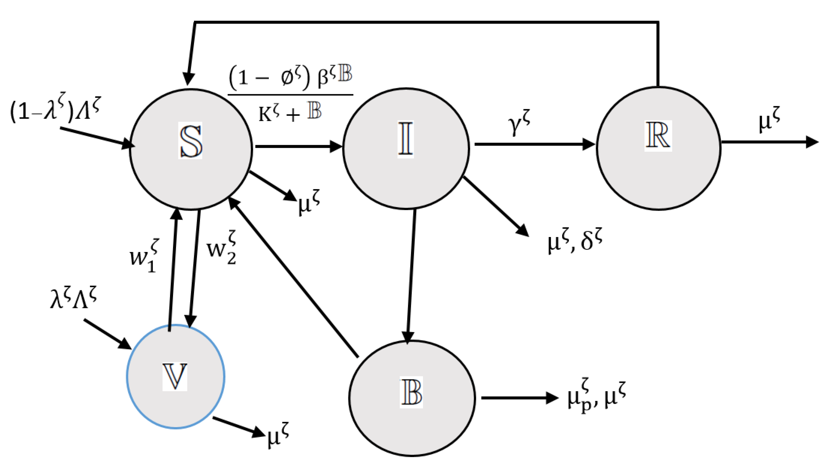
2. Mathematical Model
- Susceptible (): This group represents individuals at risk of acquiring acute diarrhea infection.
- Infected (): This group represents individuals who have been infected and are exhibiting symptoms of the infection.
- Vaccination (): This group represents individuals who have received vaccination against the infection.
- Recovery (): This group represents individuals who have recovered from the infection and are no longer exhibiting symptoms. However, they may still be susceptible to contracting the disease again.
- Bacteria (): This group represents the concentration of bacteria associated with the infection. It interacts with the susceptible population , leading to infection through a nonlinear incidence rate known as the force of infection
3. Crossover Behavior
4. Mathematical Properties of the Model (1)
4.1. Existence and Uniqueness of Solutions
4.2. Boundedness and Positivity of the Solutions
4.3. Basic Reproduction Number
4.4. Local and Global Stability of DFE Point
5. The Fractional Optimal Control Model
6. Optimality Model
7. Sensitivity Analysis
8. Numerical Scheme of Fractional Optimal Control Model with pmABC Fractional Derivative
9. Simulation and Comparative Results
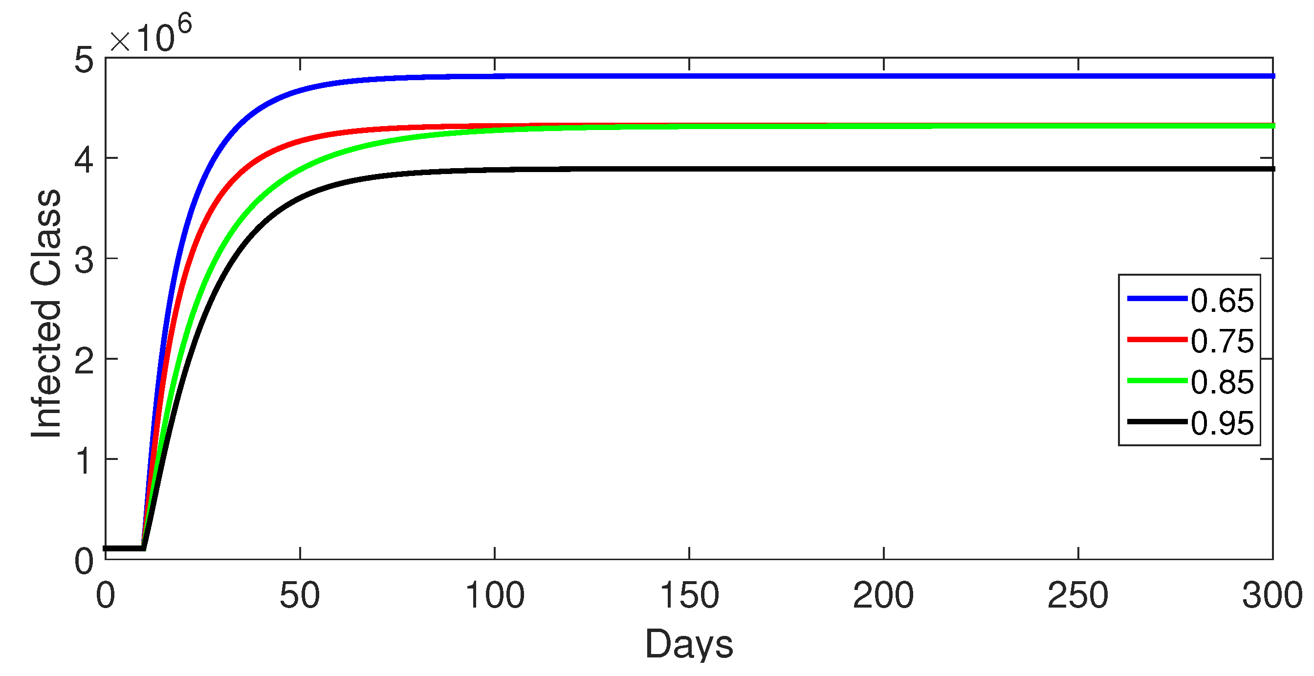
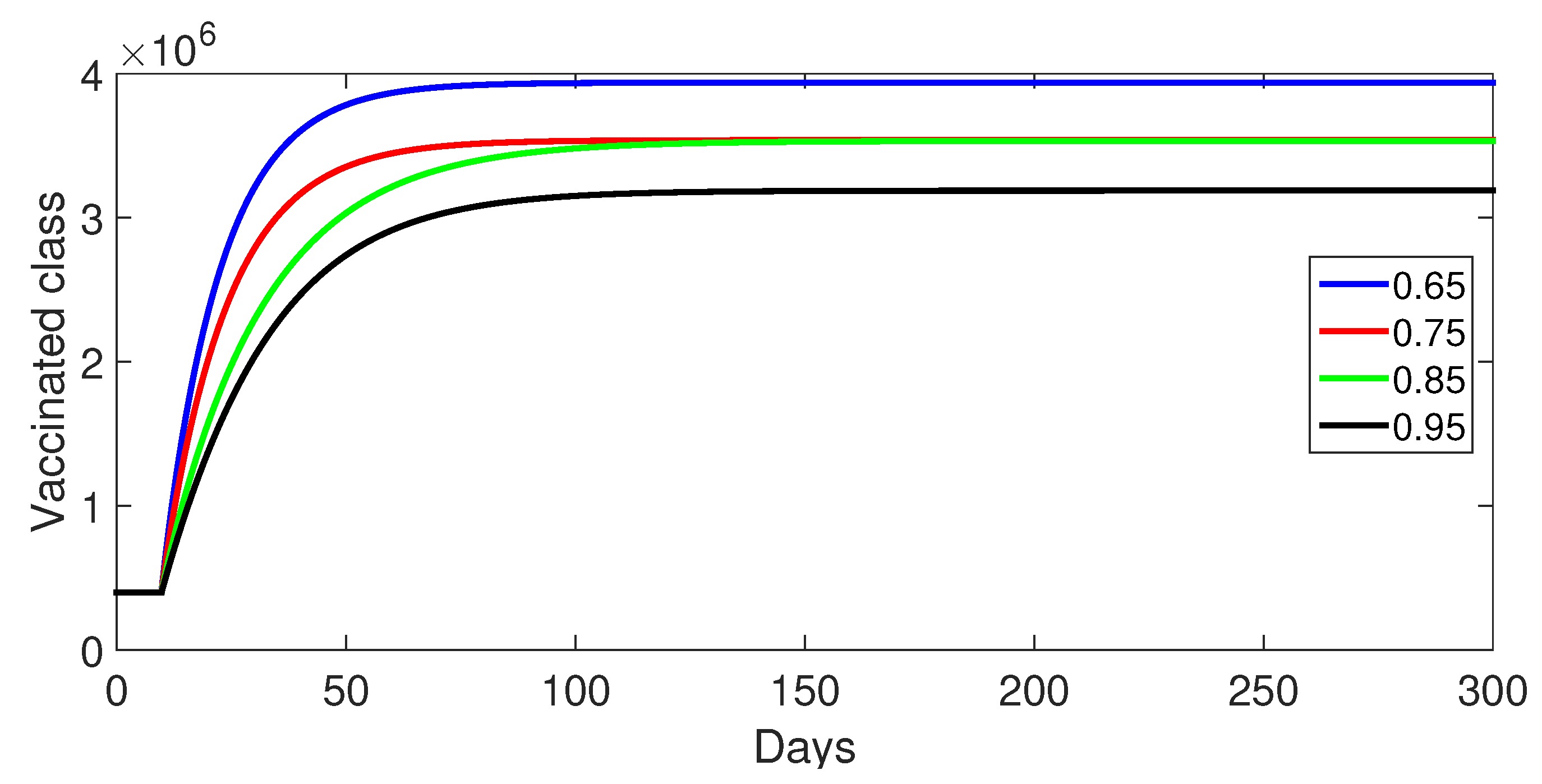
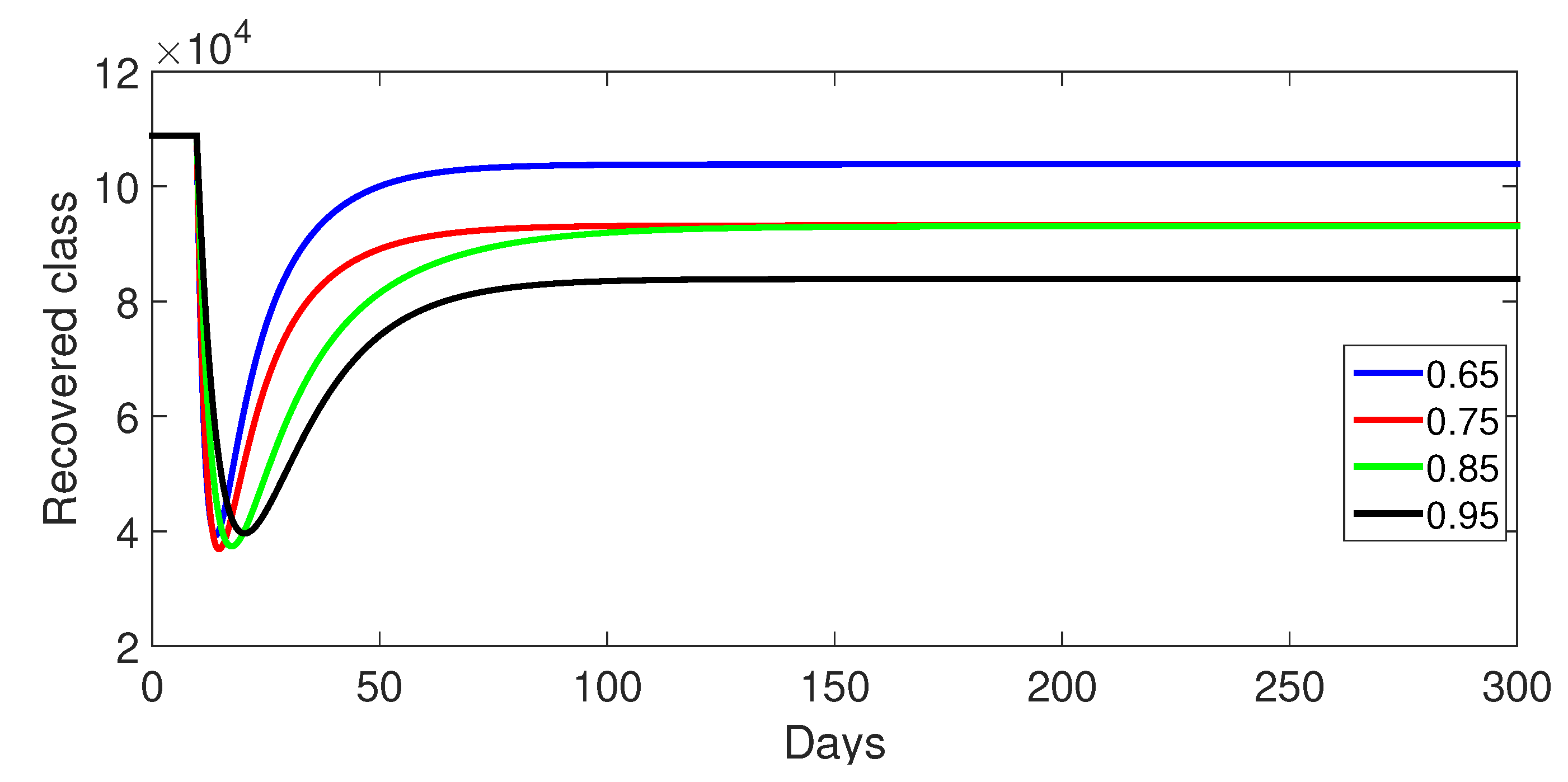
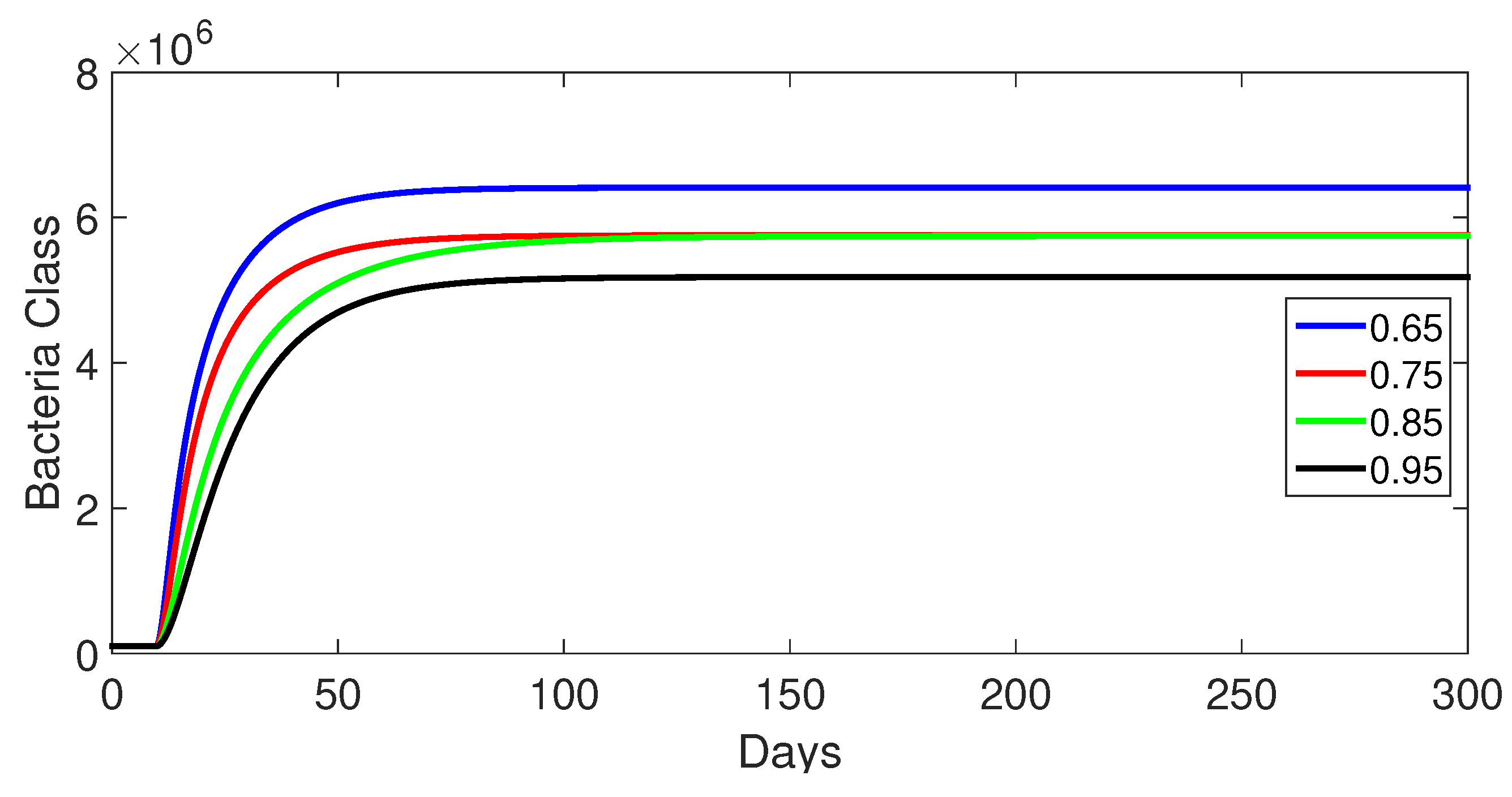
9.1. Case 1: (Without Control)
9.2. Case 2: and (Without Control )
9.3. Case 3: and (Without Control )
9.4. Comparison Between Classes Without and with Control
10. Discussion
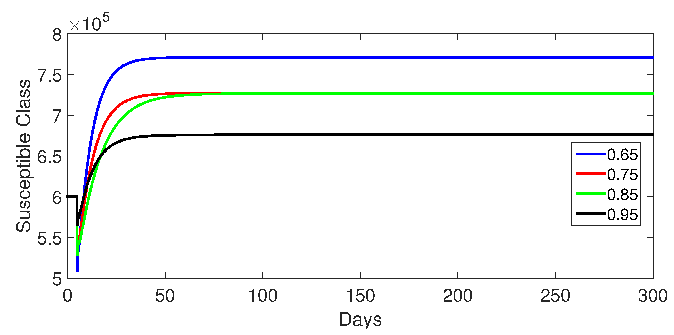
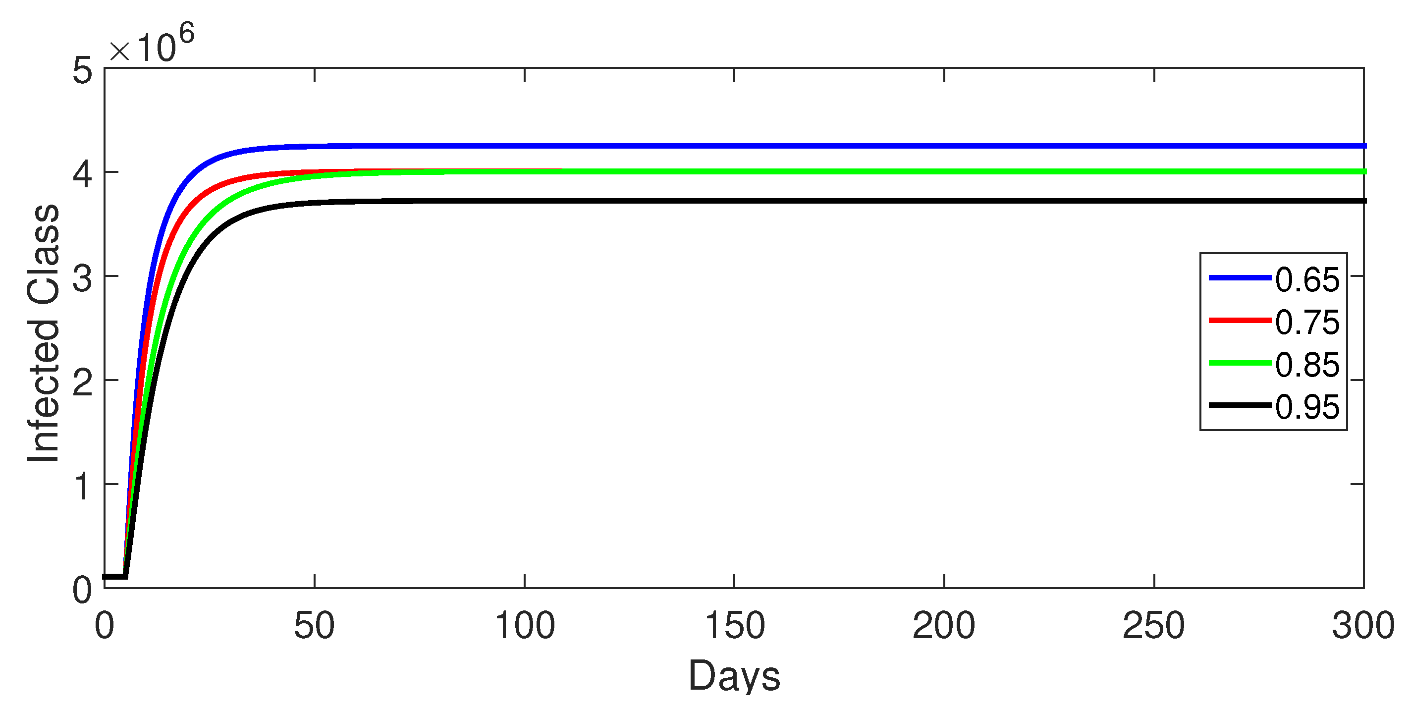
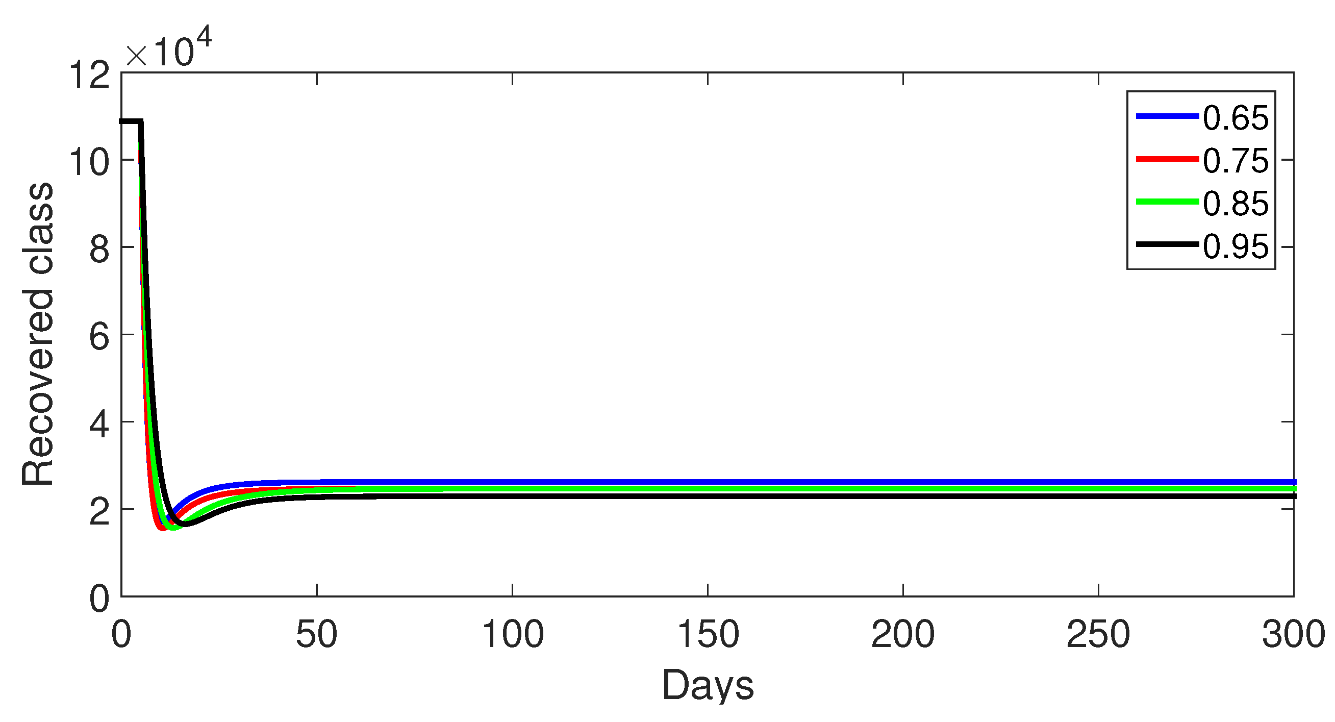
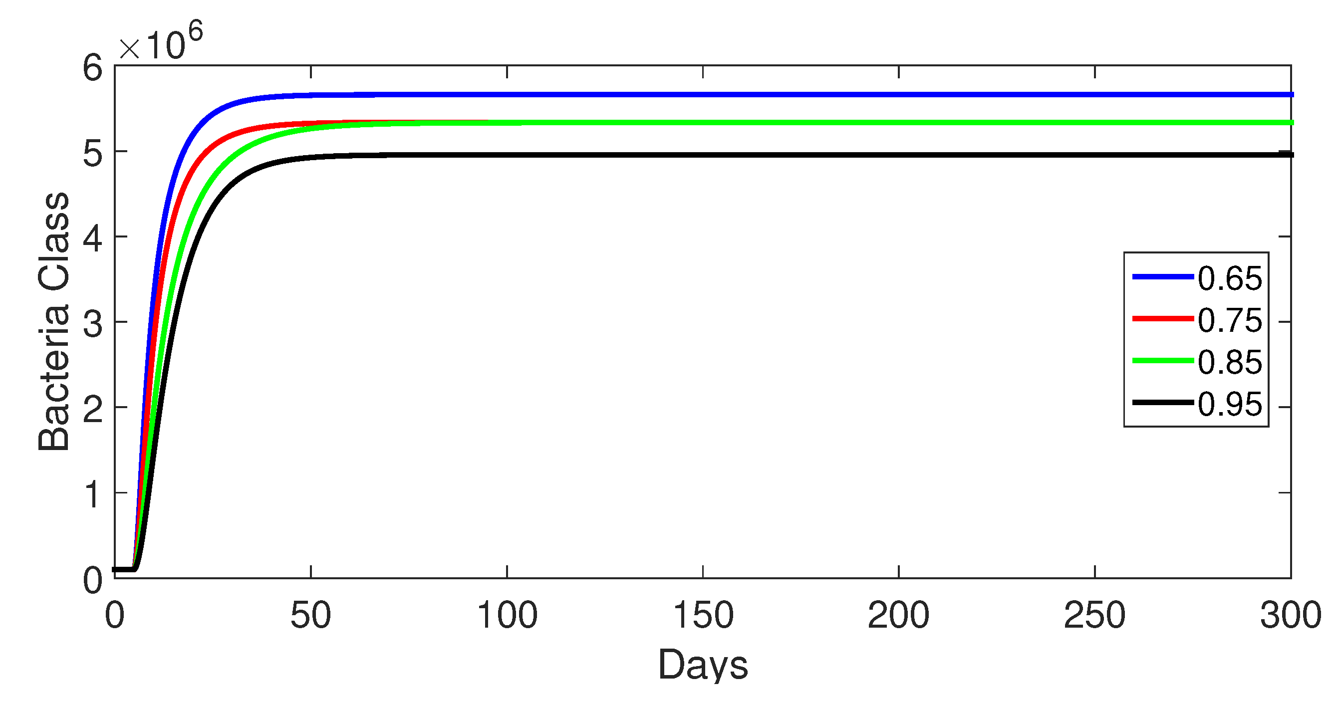
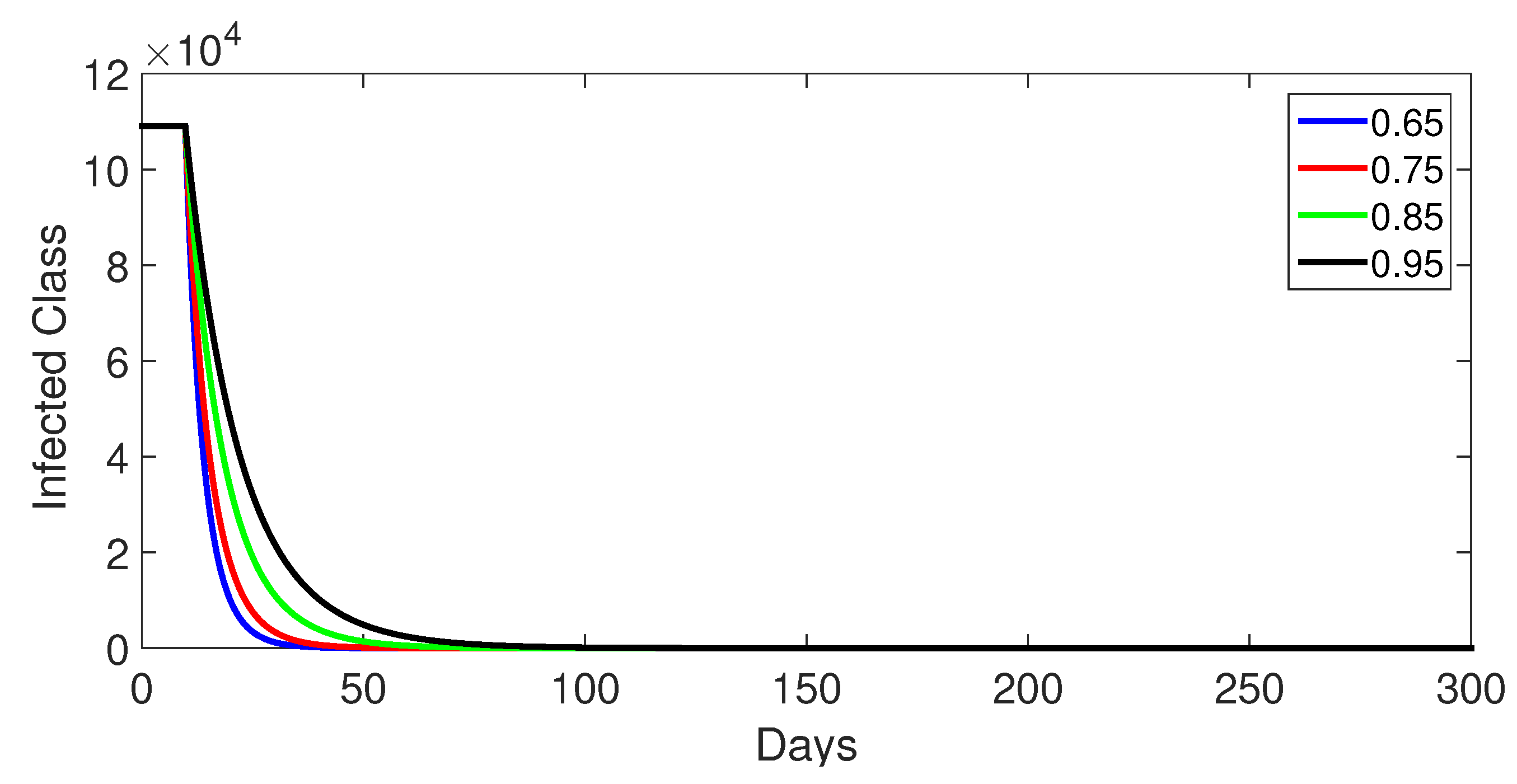
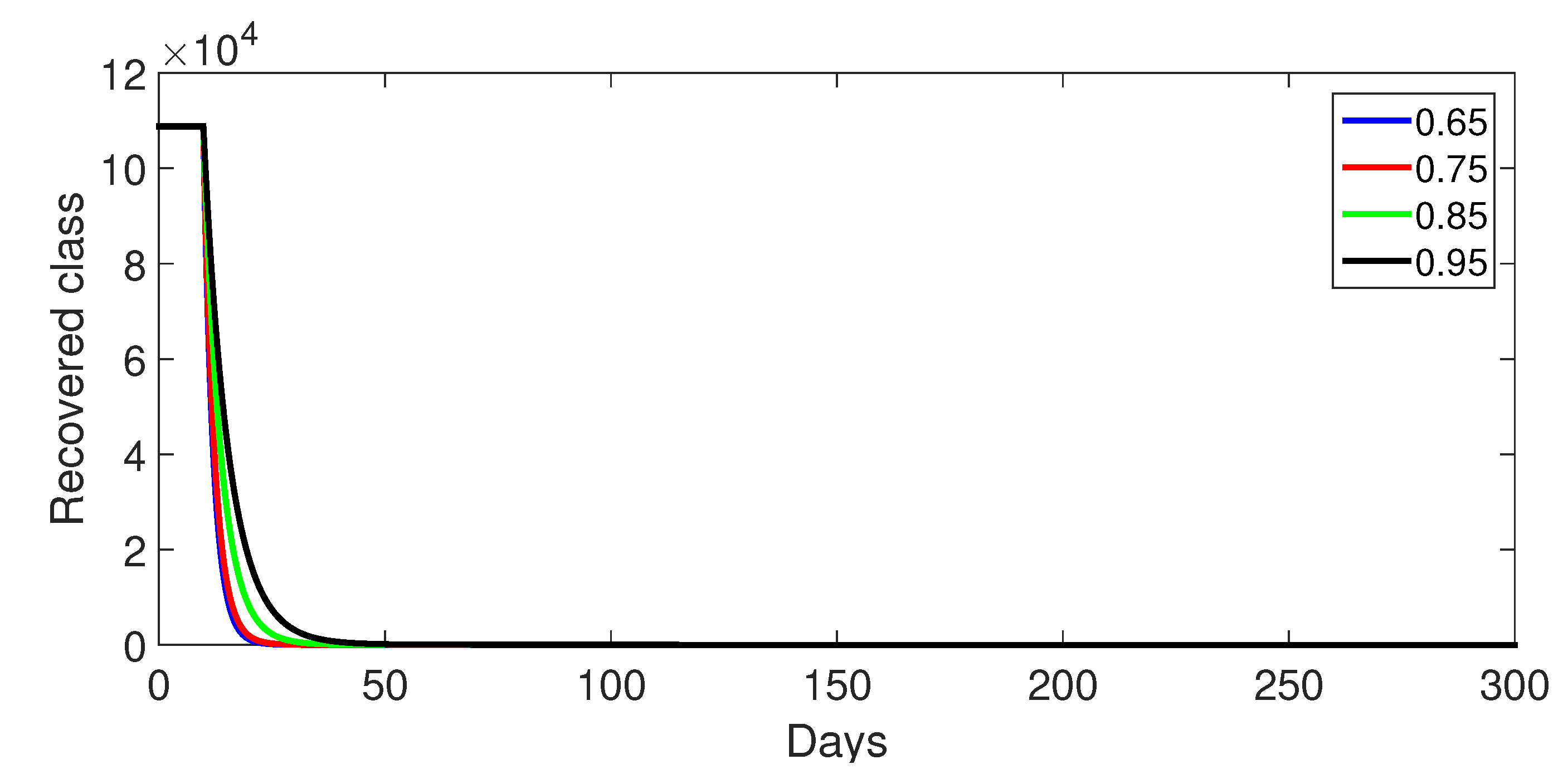
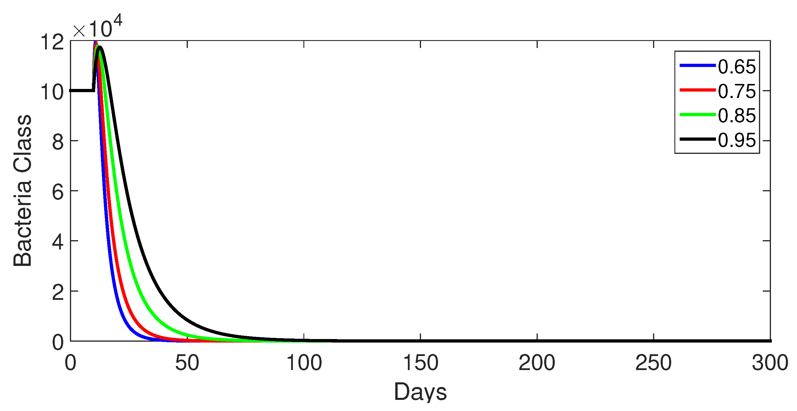
- Case 1: Without control, with (Figure 2, Figure 3, Figure 4, Figure 5 and Figure 6). In the absence of any control measures, the acute diarrhea model demonstrates an initial rise in susceptible individuals before their numbers peak and decline, stabilizing as the infection spreads. Concurrently, the infected, vaccinated, and recovered populations rapidly increase and reach steady-state levels, alongside a sharp increase in bacterial load. Notably, lower values of the fractional order parameter () are associated with higher levels of infection, vaccination, recovery, and bacterial concentration, indicating its influence on the overall scale of the outbreak.Biological Implications:Unmitigated Outbreak: This case demonstrates what an outbreak looks like without interventions. The model shows the rapid rise of infection, followed by a stabilization of population as the number of individuals in each class becomes steady.Impact of Fractional Order: The fractional order seems to have an impact on the overall size of each class. For example, lower fractional order values result in a higher bacterial load, which can lead to more infections. This suggests that the "memory effect" captured by the fractional order plays a role in how the infection spreads.
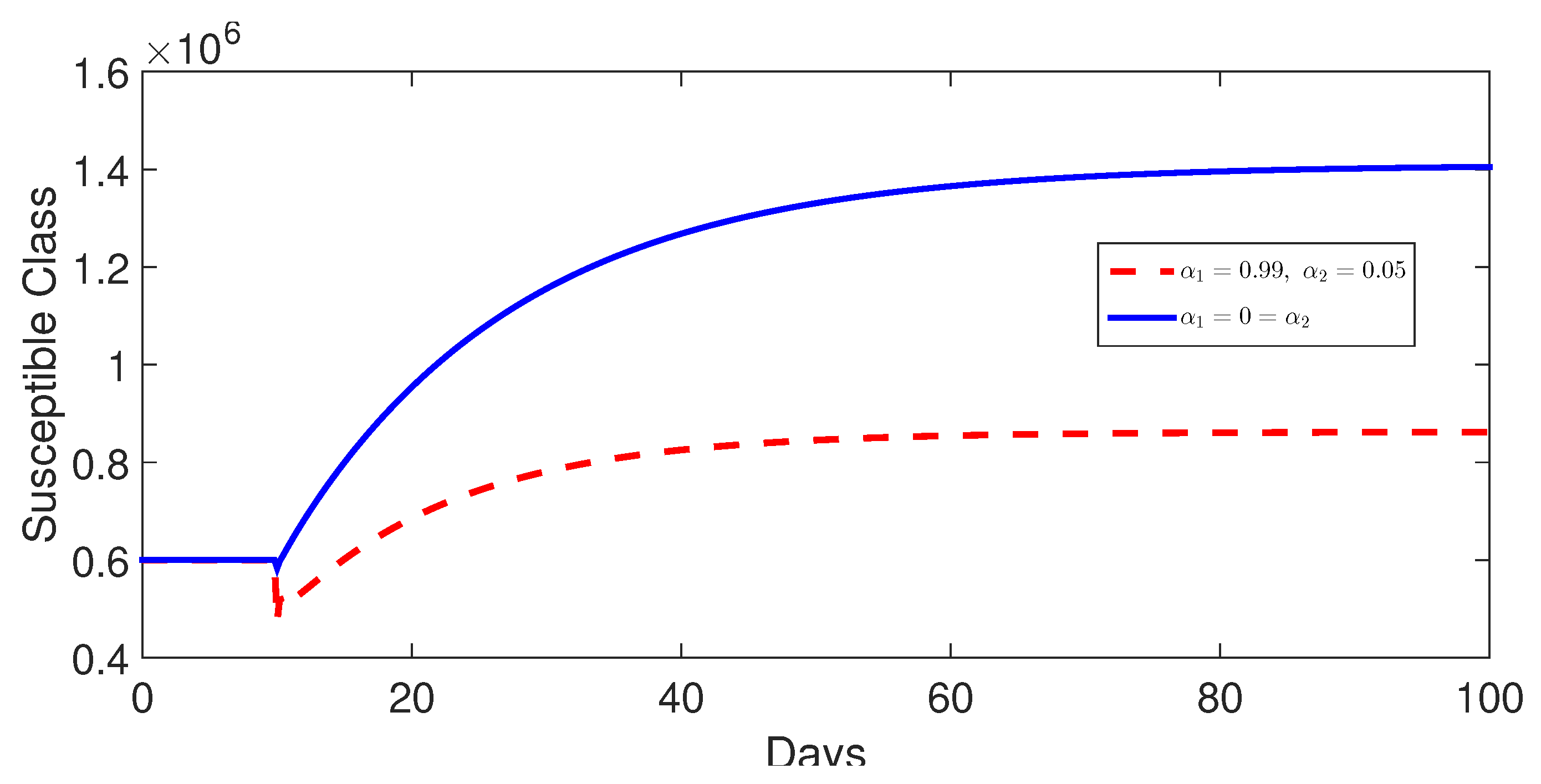
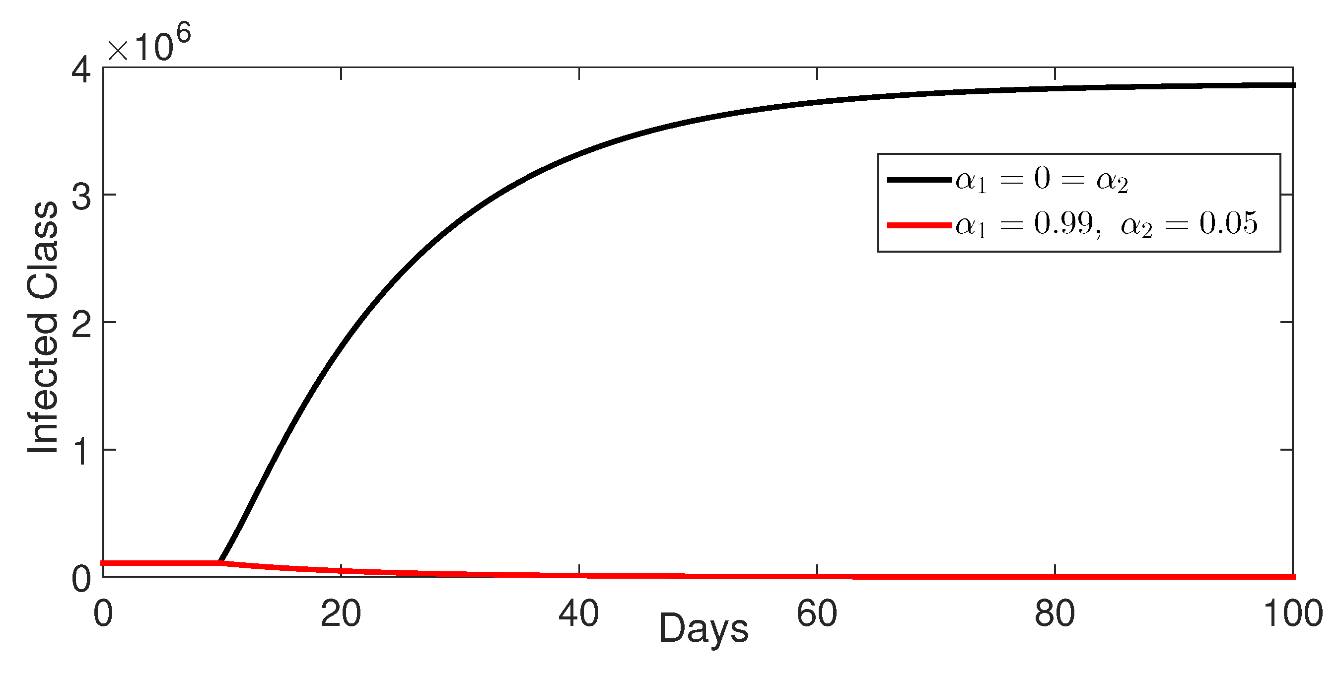
- Case 2: Control with and (without control ) (Figure 7, Figure 8, Figure 9, Figure 10 and Figure 11).Impact of Reduced Contact: The intervention of the control , which represents a measure to reduce contact between susceptible and infected individuals (e.g., implementing public health measures to encourage hand washing and sanitation), clearly shows an impact. It leads to a lower number of infections and susceptible individuals at equilibrium compared to the no-control scenario. This is expected since reducing interactions between susceptible and infected individuals reduces the possibility of transmission.Disease Reduction, Not Elimination: Despite the intervention, the disease is not eliminated. The disease will reach a steady state but at a reduced level compared to the scenario with no interventions. This means that public health measures such as sanitation are essential to reduce the disease spread but cannot eliminate it entirely.
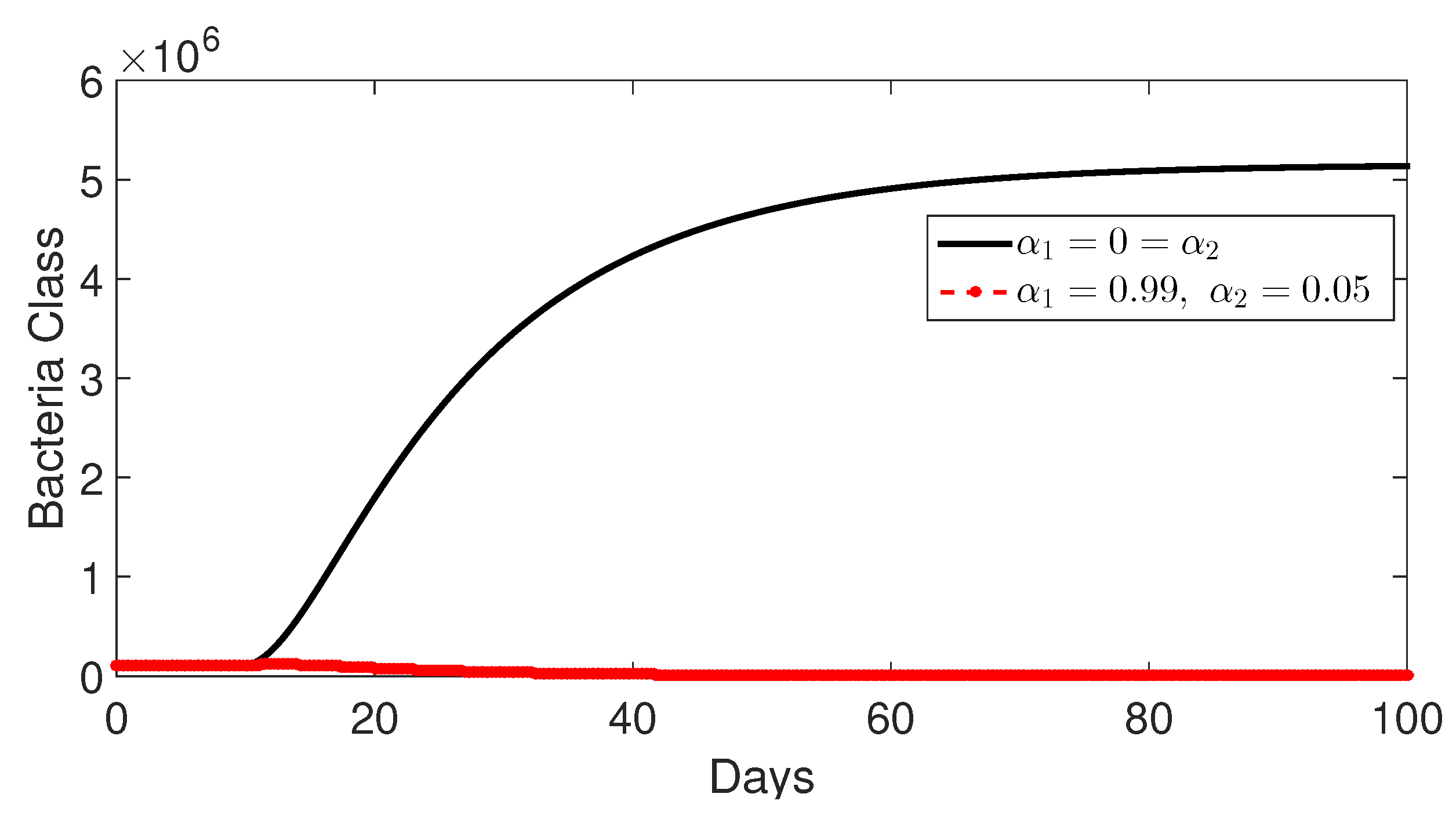
- Case 3: Control with and (without control ) (Figure 12, Figure 13, Figure 14, Figure 15 and Figure 16). The intervention of the control (), which targets the treatment of infected individuals, has a strong impact on the number of infected individuals. The model shows that treatment has the biggest impact on disease dynamics, as it reduces the overall number of infections compared to the intervention that reduces contact.Higher Recovery: This scenario clearly shows that treatment reduces infection numbers and increases the number of recovered individuals. This demonstrates the importance of treating patients to reduce both infections and transmission.Bacterial Load Reduction: The model shows that treatment reduces the bacterial load in the environment. This is consistent with reality since reducing the duration of infection would reduce bacterial production and environmental load.
11. Strategies
- Preventative Contact Control: Implement public health measures to minimize contact between susceptible individuals and the bacterial sources, utilizing sanitation, hygiene campaigns, and source reduction methods.
- Targeted Treatment: Ensure timely access to treatment for all individuals exhibiting symptoms, bolstering health infrastructures to achieve maximum effect. Integrated Intervention: Employ combined prevention and treatment approaches, using both sanitation and individual treatment strategies, for the optimized control of disease levels.
- Resource Allocation: Allocate sufficient resources to support preventative and treatment interventions, including strengthening the healthcare infrastructure and increasing public health programs.
- Community Engagement: Implement campaigns and programs with community involvement to ensure proper engagement with all health policies.
12. Conclusions
Author Contributions
Funding
Data Availability Statement
Acknowledgments
Conflicts of Interest
References
- Aldwoah, K.A.; Almalahi, M.A.; Abdulwasaa, M.A.; Shah, K.; Kawale, S.V.; Awadalla, M.; Alahmadi, J. Mathematical analysis and numerical simulations of the piecewise dynamics model of Malaria transmission: A case study in Yemen. AIMS Math. 2024, 9, 4376–4408. [Google Scholar] [CrossRef]
- Aldwoah, K.A.; Almalahi, M.A.; Shah, K. Theoretical and numerical simulations on the hepatitis B virus model through a piecewise fractional order. Fractal Fract. 2023, 7, 844. [Google Scholar] [CrossRef]
- Sweilam, N.H.; Al-Mekhlafi, S.M.; Assiri, T.; Atangana, A. Optimal control for cancer treatment mathematical model using Atangana–Baleanu–Caputo fractional derivative. Adv. Differ. Equa. 2020, 2020, 334. [Google Scholar] [CrossRef]
- Naveed, M.; Raza, A.; Soori, A.H.; Inc, M.; Rafiq, M.; Ahmed, N.; Iqbal, M.S. A dynamical study of diarrhea delayed epidemic model: Application of mathematical biology in infectious diseases. Eur. Phys. J. Plus 2023, 138, 664. [Google Scholar] [CrossRef]
- Wang, W.; Liu, T.; Fan, X. Mathematical modelling of cholera disease with seasonality and human behavior change. Discret Contin. Dyn. Syst. B 2024, 29, 3531–3556. [Google Scholar] [CrossRef]
- Ahmad, A.; Farman, M.; Akgül, A.; Nissar, K.S.; Abdel-Aty, A.H. Mathematical Analysis of Fractional Order Diarrhea Model. Progr. Fract. Differ. Appl 2023, 9, 41–58. [Google Scholar]
- Atangana, A.; Baleanu, D. New fractional derivatives with nonlocal and non-singular kernel: Theory and application to heat transfer model. Therm. Sci. 2016, 20, 763. [Google Scholar] [CrossRef]
- Alazman, I.; Alkahtani, B.S.T. Investigation of Novel Piecewise Fractional Mathematical Model for COVID-19. Fractal Fract. 2022, 6, 661. [Google Scholar] [CrossRef]
- Uçar, E.; Özdemir, N. New fractional cancer mathematical model via IL-10 cytokine and anti-PD-L1 inhibitor. Fractal Fract. 2023, 7, 151. [Google Scholar] [CrossRef]
- Addai, E.; Adeniji, A.; Peter, O.J.; Agbaje, J.O.; Oshinubi, K. Dynamics of age-structure smoking models with government intervention coverage under fractal-fractional order derivatives. Fractal Fract. 2023, 7, 370. [Google Scholar] [CrossRef]
- Riabi, L.; Hamdi Cherif, M.; Cattani, C. An Efficient Approach to Solving the Fractional SIR Epidemic Model with the Atangana-Baleanu-Caputo Fractional Operator. Fractal Fract. 2023, 7, 618. [Google Scholar] [CrossRef]
- Berhe, H.W.; Qureshi, S.; Shaikh, A.A. Deterministic modeling of dysentery diarrhea epidemic under fractional Caputo differential operator via real statistical analysis. Chaos Solitons Fractals 2020, 131, 109536. [Google Scholar] [CrossRef]
- Iqbal, M.S.; Ahmed, N.; Akgül, A.; Raza, A.; Shahzad, M.; Iqbal, Z.; Malik, M.R.; Jarad, F. Analysis of the fractional diarrhea model with Mittag-Leffler kernel. AIMS Math. 2022, 7, 13000–13018. [Google Scholar] [CrossRef]
- Lasisi, N.O.; Akinwande, N.I.; Abdulrahaman, S. Optimal control and effect of poor sanitation on modelling the acute diarrhea infection. J. Complex. Health Sci. 2020, 3, 91–103. [Google Scholar] [CrossRef]
- Qureshi, S.; Atangana, A. Fractal-fractional differentiation for the modeling and mathematical analysis of nonlinear diarrhea transmission dynamics under the use of real data. Chaos Solitons Fractals 2020, 136, 109812. [Google Scholar] [CrossRef]
- Atangana, A.; Araz, S.I. New concept in calculus: Piecewise differential and integral operators. Chaos Solitons Fract. 2021, 145, 110638. [Google Scholar] [CrossRef]
- Al-Refai, M.; Baleanu, D. On an extension of the operator with Mittag-Leffler kernel. Fractals 2022, 30, 2240129. [Google Scholar] [CrossRef]
- Aldwoah, K.A.; Almalahi, M.A.; Hleili, M.; Alqarni, F.A.; Aly, E.S.; Shah, K. Analytical study of a modified-ABC fractional order breast cancer model. J. Appl. Math. Comput. 2024, 70, 3685–3716. [Google Scholar] [CrossRef]
- Saber, H.; Almalahi, M.A.; Albala, H.; Aldwoah, K.; Alsulami, A.; Shah, K.; Moumen, A. Investigating a Nonlinear Fractional Evolution Control Model Using W-Piecewise Hybrid Derivatives: An Application of a Breast Cancer Model. Fractal Fract. 2024, 8, 735. [Google Scholar] [CrossRef]
- Khan, H.; Alzabut, J.; Gómez-Aguilar, J.F.; Alkhazan, A. Essential criteria for existence of solution of a modified-ABC fractional order smoking model. Ain Shams Eng. J. 2024, 15, 102646. [Google Scholar] [CrossRef]
- Aly, E.S.; Almalahi, M.A.; Aldwoah, K.A.; Shah, K. Criteria of existence and stability of an n-coupled system of generalized Sturm-Liouville equations with a modified ABC fractional derivative and an application to the SEIR influenza epidemic model. AIMS Math. 2024, 9, 14228–14252. [Google Scholar] [CrossRef]
- Ahmad, S.; Yassen, M.F.; Alam, M.M.; Alkhati, S.; Jarad, F.; Riaz, M.B. A numerical study of dengue internal transmission model with fractional piecewise derivative. Results Phys. 2022, 39, 105798. [Google Scholar] [CrossRef]
- Heydari, M.H.; Razzaghi, M.; Baleanu, D. A numerical method based on the piecewise Jacobi functions for distributed-order fractional Schrödinger equation. Commun. Nonlinear Sci. Numer. Simul. 2023, 116, 106873. [Google Scholar] [CrossRef]
- Abdelmohsen, S.A.M.; Yassen, M.F.; Ahmad, S.; Abdelbacki, A.M.M.; Khan, J. Theoretical and numerical study of the rumours spreading model in the framework of piecewise derivative. Eur. Phys. J. Plus 2022, 137, 738. [Google Scholar] [CrossRef]
- Xu, C.; Liu, Z.; Pang, Y.; Akgul, A.; Baleanu, D. Dynamics of HIV-TB coinfection model using classical and Caputo piecewise operator: A dynamic approach with real data from South-East Asia, European and American regions. Chaos Solitons Fract. 2022, 165, 112879. [Google Scholar] [CrossRef]
- Almalahi, M.A.; Aldwoah, K.A.; Shah, K.; Abdeljawad, T. Stability and Numerical Analysis of a Coupled System of Piecewise Atangana–Baleanu Fractional Differential Equations with Delays. Qual. Theory Dyn. Syst. 2024, 3, 105. [Google Scholar] [CrossRef]
- Eiman, K.S.; Sarwar, M.; Abdeljawad, T. On rotavirus infectious disease model using piecewise modified ABC fractional order derivative. NHM 2024, 19, 214–234. [Google Scholar] [CrossRef]
- van den Driessche, P.; Watmough, J. Reproduction numbers and sub-threshold endemic equilibria for compartmental models of disease transmission. Math. Biosci. 2002, 180, 29–48. [Google Scholar] [CrossRef] [PubMed]
- Bonyah, E.; Sagoe, A.K.; Kumar, D.; Deniz, S. Fractional optimal control dynamics of coronavirus model with Mittag–Leffler law. Ecol. Complex. 2021, 45, 100880. [Google Scholar] [CrossRef]


| Variable | Definition |
|---|---|
| Number of susceptible individuals at time . | |
| Number of individuals infected and showing symptoms of the infection. | |
| Number of individuals who have been vaccinated against the infection. | |
| Number of individuals who have recovered from the infection |
| Parameter | Definition of Parameter | Value | Units |
|---|---|---|---|
| Rate of human populations | 100 | day−1 | |
| Rate of immune decline in vaccinated individuals | 0.55 | day−1 | |
| Rate of recovered humans becoming susceptible | 0.003 | day−1 | |
| Vaccination rate among individuals | 0.45 | day−1 | |
| Contaminated food and water exposure rate | 0.9 | day−1 | |
| Rate of compliance with water and food hygiene practices | 0.6 | day−1 | |
| Recovery rate of infected humans | 0.002 | day−1 | |
| Bacterial infection transmission rate from infected humans | 0.8 | cell/mL/day | |
| Natural human mortality | 0.0247 | day−1 | |
| Mortality rate caused by the disease | 0.052 | day−1 | |
| Proportion of unvaccinated individuals | 0.075 | day−1 | |
| K | Bacterial concentration in contaminated water | 50,000 | |
| Mortality rate associated with bacterial infections | 0.001 | day−1 | |
| Water sanitation leading to dearth of bacteria | 0.05 | day−1 |
| Parameter | Sensitivity Value |
|---|---|
| 0.0000 | |
| −0.0762 | |
| 0.0000 | |
| 0.0762 | |
| 0.5000 | |
| −0.5000 | |
| −0.0023 | |
| 0.5000 | |
| −0.0446 | |
| −0.0286 | |
| −0.0375 | |
| K | −0.5000 |
| −0.0011 | |
| −0.0257 |
Disclaimer/Publisher’s Note: The statements, opinions and data contained in all publications are solely those of the individual author(s) and contributor(s) and not of MDPI and/or the editor(s). MDPI and/or the editor(s) disclaim responsibility for any injury to people or property resulting from any ideas, methods, instructions or products referred to in the content. |
© 2025 by the authors. Licensee MDPI, Basel, Switzerland. This article is an open access article distributed under the terms and conditions of the Creative Commons Attribution (CC BY) license (https://creativecommons.org/licenses/by/4.0/).
Share and Cite
Madani, Y.A.; Almalahi, M.A.; Osman, O.; Muflh, B.; Aldwoah, K.; Mohamed, K.S.; Eljaneid, N. Analysis of an Acute Diarrhea Piecewise Modified ABC Fractional Model: Optimal Control, Stability and Simulation. Fractal Fract. 2025, 9, 68. https://doi.org/10.3390/fractalfract9020068
Madani YA, Almalahi MA, Osman O, Muflh B, Aldwoah K, Mohamed KS, Eljaneid N. Analysis of an Acute Diarrhea Piecewise Modified ABC Fractional Model: Optimal Control, Stability and Simulation. Fractal and Fractional. 2025; 9(2):68. https://doi.org/10.3390/fractalfract9020068
Chicago/Turabian StyleMadani, Yasir A., Mohammed A. Almalahi, Osman Osman, Blgys Muflh, Khaled Aldwoah, Khidir Shaib Mohamed, and Nidal Eljaneid. 2025. "Analysis of an Acute Diarrhea Piecewise Modified ABC Fractional Model: Optimal Control, Stability and Simulation" Fractal and Fractional 9, no. 2: 68. https://doi.org/10.3390/fractalfract9020068
APA StyleMadani, Y. A., Almalahi, M. A., Osman, O., Muflh, B., Aldwoah, K., Mohamed, K. S., & Eljaneid, N. (2025). Analysis of an Acute Diarrhea Piecewise Modified ABC Fractional Model: Optimal Control, Stability and Simulation. Fractal and Fractional, 9(2), 68. https://doi.org/10.3390/fractalfract9020068