A Novel Approach for Solving Fractional Differential Equations via a Multistage Telescoping Decomposition Method

Abstract

This study presents a novel algorithm for solving nonlinear fractional initial value problems, utilizing a multistage telescoping decomposition method (FTDM). By combining the MFTDM with the Elzaki transform, this method significantly improves computational efficiency and accuracy. Through a series of numerical experiments, the proposed approach is demonstrated to be highly practical, reliable and straightforward, offering a robust framework for solving nonlinear fractional differential equations effectively.

1. Introduction and Mathematical Preliminaries

Fractional differential equations (FDEs) have gained prominence in modeling complex systems exhibiting memory-dependent and nonlocal characteristics, such as those found in fluid mechanics, viscoelastic materials, biology and physics. These equations provide a comprehensive approach to phenomena that classical integer-order differential equations cannot capture adequately.

However, obtaining exact solutions for FDEs remains challenging, prompting researchers to explore numerical and analytical techniques for their solution. Notable methods include the Adomian decomposition method (ADM) [1], the variational iteration method (VIM), the Decompostion method [2,3] and the Homotopy perturbation method (HPM) [4,5], which are often coupled with integral transforms like the Laplace transform [6,7,8], Sumudu transform [9,10,11,12], Elzaki transform [13,14,15,16,17], ZZ transform [2,3,8,12,13,14,15,16,17,18,19,20,21,22,23,24,25,26], Aboodh transform [27], ARA transform [24], Natural Transform [28] and New Double Kharrat-Toma [29] to enhance their efficiency.

The telescoping decomposition method TDM was initially introduced in [19,21] for solving ordinary differential equations. This method, grounded in the Taylor series expansion, aims to construct an analytical solution in the form of a polynomial. One significant advantage of the telescoping decomposition method is that it eliminates the need to compute Adomian polynomials, thus offering a simpler alternative to the Adomian method. In [30], the author explores the multistage telescoping decomposition method for solving fractional differential equations. In [31], they employed the multistage telescoping decomposition method to give a solution for a system of nonlinear fractional differential equations.

In this paper, a multistage telescoping decomposition method (MFTDM) is proposed to solve nonlinear fractional differential and partial differential equations. This method builds upon the existing MFTDEM by integrating the Elzaki transform, thereby improving its computational efficiency and simplifying the solution process and thus offering a more straightforward and efficient computational procedure.

The multistage telescoping decomposition Elzaki method is known for its accuracy and fast convergence, making it ideal for solving complex nonlinear equations. By breaking the problem into multiple stages, it improves control over the solution process and reduces computational time. Despite these advantages, the method can face challenges such as computational complexity, requiring a delicate balance between accuracy and performance efficiency. Nevertheless, it remains effective for tackling large-scale mathematical problems with multiple variables.

The remainder of this paper is organized as follows: Section 2 introduces the foundational concepts of fractional calculus and the Elzaki transform. Section 3 presents the new algorithm for solving nonlinear fractional differential equations. Finally, Section 4 provides a conclusion, highlighting the effectiveness of the proposed method and suggesting avenues for future research.

2. Fundamental Definitions

This section covers some essential backgrounds in fractional calculus, particularly the fractional derivative, fractional integral and some definitions and properties of the Elzaki transform.

2.1. Fractional Calculus

We introduce some basic definitions and properties of fractional calculus using the Riemann–Liouville fractional integrals and Caputo fractional derivatives [32].

Theorem 1

([32]). If $h\left(\tau \right)\in A{C}^n[a,b]$, then the Caputo fractional derivative ${(}^c{D}_{0^{+}}^{\rho })\left(\tau \right)$ exists almost everywhere on $[a,b]$. If $\rho \notin \mathbb{N}$, then ${(}^c{D}_{0^{+}}^{\rho })\left(\tau \right)$ is represented by

$${(}^c{D}_{0^{+}}^{\rho }h)\left(\tau \right)={\displaystyle \frac{1}{\Gamma (n-\rho )}}{\int }_0^{\tau }{\displaystyle \frac{h^{\left(n\right)}\left(\zeta \right)d\zeta }{{(\tau -\zeta )}^{\rho -n+1}}},$$

(1)

where Γ is the Gamma function.

Remark 1

([32]). We consider the time-fractional derivative in the Caputo sense. When $\rho \in {\mathbb{R}}_{+}$, the time-fractional derivative is defined as

$$\begin{array}{cc}\hfill {(}^c{D}_{0^{+}}^{\rho }h)\left(\tau \right)& ={\displaystyle \frac{{\partial }^{\rho }h\left(\tau \right)}{\partial {\tau }^{\rho }}}\hfill \\ \hfill & =\left\{\begin{array}{c}{\displaystyle \frac{1}{\Gamma (m-\rho )}}{\int }_0^{\tau }{(\tau -\zeta )}^{m-\rho -1}{\displaystyle \frac{{\partial }^{m}h\left(\zeta \right)d\zeta }{\partial {\tau }^m}},m-1<\rho <m\hfill \\ {\displaystyle \frac{{\partial }^{m}h\left(\tau \right)}{\partial {\tau }^m}},\rho =m.\hfill \end{array}\right.\hfill \end{array}$$

(2)

where $m\in {\mathbb{N}}^{*}$.

Definition 1

([32]). Let $\rho \in {\mathbb{R}}_{+}$. The operator $I_a^{\rho }$ defined on $L_1[a,b]$ by

$$\left(I_{0^{+}}^{\rho }h\right)\left(\tau \right)={\displaystyle \frac{1}{\Gamma \left(\rho \right)}}{\int }_0^{\tau }{(\tau -\zeta )}^{\rho -1}h\left(\zeta \right)d\zeta ;\rho >0,$$

(3)

is called the Riemann–Liouville fractional integral operator of order ρ. Here, $\Gamma (.)$ is the Gamma function.

2.2. Properties and Definition of Elzaki Transform

The Elzaki transform is a novel integral transform specifically designed for functions of exponential order. It is applied to functions within the set H as described in [15]. This transform is instrumental in simplifying fractional differential equations and enhancing their solvability by reducing their complexity.

$$H=\left\{h\left(\tau \right):\exists Q,{\lambda }_1,{\lambda }_2>0,\left|h\left(\tau \right)\right|<Q{e}^{{\displaystyle \frac{\left|\tau \right|}{{\lambda }_i}}},if\tau \in {(-1)}^i\times [0,\infty ),h\in A{C}^n\left(\mathbb{R}\right)\right\}.$$

(4)

We introduce a new Elzaki transform which is defined in (4) by

$$E\left[h\left(\tau \right)\right]=T\left(s\right)=s{\int }_0^{\infty }h\left(\tau \right)e^{-{\displaystyle \frac{\tau }{s}}}d\tau .$$

(5)

Next, the inverse of the Elzaki transform is denoted by $E^{-1}\left[T\left(s\right)\right]=h\left(\tau \right),\tau \ge 0$. When $\rho$ is a fractional number, we have

$$E\left[{\tau }^{\rho }\right]=\Gamma (\rho +1)s^{\rho +2}.$$

We will summarize some results of the Elzaki transform for some functions [15] in

Table 1. Elzaki transform of some functions.

$\mathit{h}\left(\mathit{\tau }\right)$	$\mathit{E}\left[\mathit{h}\right(\mathit{\tau }\left)\right]$	$\mathit{h}\left(\mathit{\tau }\right)$	$\mathit{E}\left[\mathit{h}\right(\mathit{\tau }\left)\right]$
1	$v^2$	$sin\left(a\tau \right)$	${\displaystyle \frac{a{v}^3}{1+a^2{v}^2}}$
$\tau$	$v^3$	$cos\left(a\tau \right)$	${\displaystyle \frac{v^2}{1+a^2{v}^2}}$
${\tau }^n,n\ge 0$	$n!v^{n+2}$	$e^{a\tau }$	${\displaystyle \frac{v^2}{1-av}}$
${\displaystyle \frac{{\tau }^{\rho -1}}{\Gamma \left(\rho \right),\rho \succ 0}}$	$v^{\rho +1}$	$M(t-a)$	$v^2{e}^{-{\displaystyle \frac{a}{v}}}$

.

Theorem 2

([15]). The Elzaki transform amplifies the coefficients of the power series function

$$h\left(\tau \right)=\sum _{n=0}^{\infty }{a}_n{\tau }^n,$$

(6)

on the new integral transform Elzaki transform, given by

$$E\left[h\left(\tau \right)\right]=T\left(v\right)=\sum _{n=0}^{\infty }n!a_n{v}^{n+2}.$$

(7)

Theorem 3

([15]). Let $h\left(\tau \right)$ be in H and $T_n\left(v\right)$ denote Elzaki transform of the nth derivative $h^{\left(n\right)}\left(\tau \right)$ of $h\left(\tau \right)$, Then, for $n\ge 1$,

$$T_n\left(v\right)={\displaystyle \frac{T\left(v\right)}{v^n}}-\sum _{i=0}^{n-1}{v}^{2-n+i}{h}^{\left(i\right)}\left(0\right),$$

(8)

By using the integration by parts,

$$E\left[{\displaystyle \frac{\partial h(x,\tau )}{\partial \tau }}\right]={\displaystyle \frac{1}{v}}T(x,v)-vh(x,0),$$

$$E\left[{\displaystyle \frac{{\partial }^{2}h(x,\tau )}{\partial {\tau }^2}}\right]={\displaystyle \frac{1}{v^2}}T(x,v)-vh(x,0).$$

Theorem 4

([15]). Suppose $E\left(h\right)$ is the Elzaki transform of the function $h\left(\tau \right)$. Then,   

$$E\left\{\left({}_{ }{}^{c}D_{0^{+}}^{\rho }\right)\left(\tau \right),v\right\}={\displaystyle \frac{T\left(v\right)}{v^{\rho }}}-\sum _{i=0}^{n-1}{v}^{i-\rho +2}{h}^{\left(i\right)}\left(0\right).$$

(9)

Proof. 

For the proof, see [15].    □

2.3. Algorithm of Telescoping Decomposition Method

Consider the general nonlinear fractional differential equation

$$Lu+Ru+Nu=g\left(t\right)$$

(10)

where L and N are linear and nonlinear operators, respectively, R represents the remaining linear part and g is a given function. The key idea of the FTDM [19] is to express the nonlinear term Nu as an infinite series of the nonlinear term u in the Banach space,

$$Nu\left(\tau \right)=\sum _{r=0}^{\infty }{N}_{r}u\left(\tau \right),$$

(11)

where $N_r$ can be calculated by

$$\left\{\begin{array}{cc}{\displaystyle N_{0}u\left(\tau \right)=N{u}_0\left(\tau \right),}& \\ & & \\ N_{r}u\left(\tau \right)=N{U}_r\left(\tau \right)-N{U}_{r-1}\left(\tau \right)\end{array}\right.$$

with

$$U_r\left(\tau \right)=\sum _{k=0}^r{u}_k\left(\tau \right),U_{r-1}\left(\tau \right)=\sum _{k=0}^{r-1}{u}_k\left(\tau \right),r=1,2,3,\cdots$$

and the remaining linear part $Ru$ can be written as

$$Ru\left(\tau \right)=\sum _{r=0}^{\infty }R{u}_r\left(\tau \right).$$

(12)

Multistage Telescoping Decomposition Method

The principal of the MFTDM [30] is based on the decomposition of the time interval $[0,T]$ in a sequence of subintervals, $[t_0,t_1],[t_1,t_2],\cdots [t_{M-1},t_M]$, in which $t_0=0,t_M=T$ and ${\bigcup }_0^{M-1}[t_i,t_{i+1}]=[0,T]$, where the subintervals can be chosen as the same length $\Delta$, i.e., $\Delta t_i=\Delta t,i=0,\cdots ,M-1$.

More precisely, Equation (11) can be solved by the FTDM in every sequential interval ${\Omega }_i(i=0,1,\cdots ,M-1)$. The solution of problem (10) is provided in the piecewise form; the new sequence is as follows: when ${\Omega }_0=\left[{\tau }_0,{\tau }_1\right]$,

$${\Phi }_{M_0}^0\left(\tau \right)=\sum _{k=0}^{M_0}{u}_k^0\left(\tau \right)=u_0^0\left(\tau \right)+u_1^0\left(\tau \right)\cdots +u_{M_0}^0\left(\tau \right),M_0\in \mathbb{N}-\left\{0\right\},$$

and in each interval ${\Omega }_i=\left[{\tau }_i,{\tau }_{i+1}\right]$, $(i=1,2,\cdots ,N-1)$, one puts

$$\begin{array}{ccc}\hfill u_0^i\left(\tau \right)& =& {\Phi }_{M_0}^{i-1}\left({\tau }_i\right)\hfill \\ \hfill {\Phi }_{M_0}^i\left(\tau \right)& =& \sum _{k=0}^{M_0}{u}_k^i\left(\tau \right).\hfill \end{array}$$

(13)

3. Multistage Telescoping Decomposition Elzaki Method

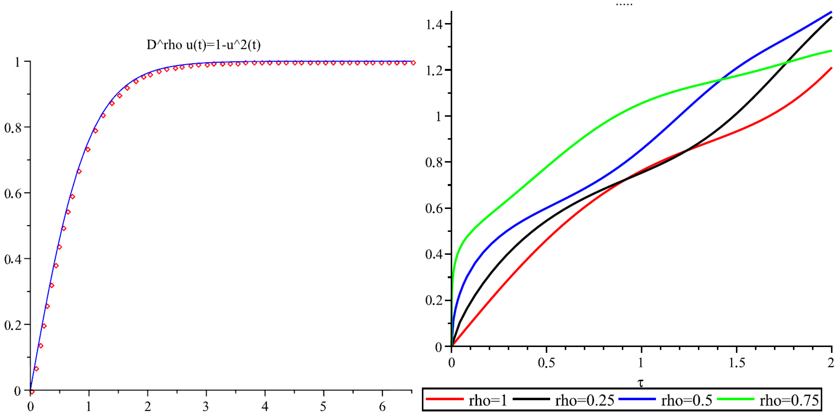
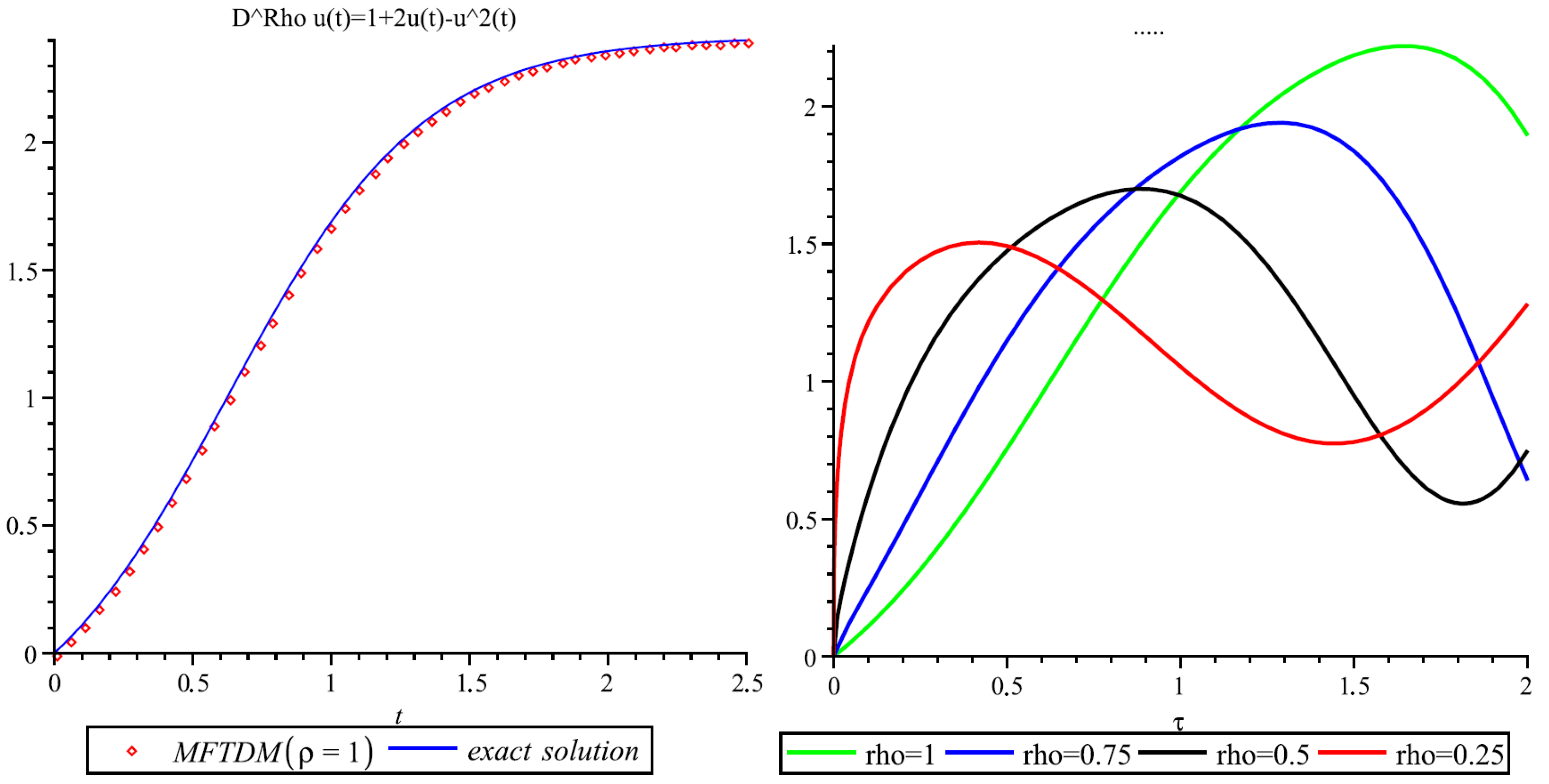
3.1. Solving the Nonlinear Fractional Differential Equations

Consider the following nonlinear fractional differential equations of order $\rho ,(m-1<\rho \le m,m=1,2,\cdots )$:   

$${}_{ }{}^{c}D_{0^{+}}^{\rho }u\left(\tau \right)+Ru\left(\tau \right)+Nu\left(\tau \right)=g\left(\tau \right)$$

(14)

and the following initial condition:

$$u^{\left(k\right)}\left(0^{+}\right)=c_k,k=0,1,2,\cdots ,m-1,$$

(15)

where ${}_{ }{}^{c}D_{0^{+}}^{\rho }$ is the Caputo fractional derivative of the function $u\left(\tau \right)$, R is the linear differential operator of less order than $L,N$ represents the general nonlinear differential operator and $g\left(t\right)$ is the source term, u, in the Banach space.

Theorem 5.

Solutions of nonlinear differential equations with the Caputo time fractional derivative, (14) and (15), using the MFTDEM are given in the form of an infinite series which converge to the exact solution of the problem (14).

Proof. 

Applying the Elzaki transform to both sides of (14), we obtain

$$E\left[D_{\tau }^{\rho }u\left(\tau \right)\right]+E\left[Ru\left(\tau \right)\right]+E\left[Nu\left(\tau \right)\right]=E\left[g\left(\tau \right)\right].$$

(16)

Using the property of the Elzaki transform, we obtain the following form:

$$E\left[u\left(\tau \right)\right]=\sum _{k=0}^{m-1}{u}^{\left(k\right)}\left(0\right)v^{2+k}+v^{\rho }[E\left[g\left(\tau \right)\right]-E\left[Ru\left(\tau \right)\right]-E\left[Nu\left(\tau \right)\right]].$$

(17)

By taking the inverse transform on each side of Equation $\left(17\right)$, it gives

$$u\left(\tau \right)=G\left(\tau \right)-E^{-1}\left\{v^{\rho }[Ru\left(\tau \right)+Nu\left(\tau \right)]\right\},$$

(18)

where $G\left(\tau \right)$ represents the terms arising from the source terms and the prescribed initial conditions. The new MTDEM represents the solution as an infinite series,

$$u\left(\tau \right)=\sum _{r=0}^{\infty }{u}_r\left(\tau \right)$$

(19)

and the nonlinear term as

$$Nu\left(\tau \right)=\sum _{r=0}^{\infty }{N}_{r}U\left(\tau \right).$$

(20)

Substituting (19) and (20) into (18), we obtain

$$\sum _{r=0}^{\infty }{u}_r\left(\tau \right)=G\left(\tau \right)-E^{-1}\left\{v^{\rho }[\sum _{r=0}^{\infty }R{u}_r\left(\tau \right)+\sum _{r=0}^{\infty }{N}_{r}U\left(\tau \right)]\right\}.$$

(21)

Comparing both sides of (21), the iterations are defined by the recursive relations

$$\begin{array}{ccc}\hfill u_0\left(\tau \right)& :=& G\left(\tau \right)\hfill \\ \hfill u_{r+1}\left(\tau \right)& :=& -E^{-1}\left\{v^{\rho }\left[R{u}_r\left(\tau \right)+N_{r}U\left(\tau \right)\right]\right\}.\hfill \\ \hfill \end{array}$$

(22)

Finally, we approximate the solution $u\left(\tau \right)$ by truncated series:

$$u\left(\tau \right)={\Phi }_M\left(\tau \right)=\sum _{k=0}^M{u}_k\left(\tau \right).$$

(23)

In this part, we will prove that ${\sum }_{r=0}^{\infty }{u}_r\left(\tau \right)$ converges on the interval $[0,T]$ to the exact solution of Equations (14) and (15), if $0<\alpha \le 1$. Suppose the sequence of functions $u_r\left(\tau \right)$ and $u\left(\tau \right)$ are defined in a Banach space $C\left([0,T],\parallel .\parallel \right)$ and $\left\{B_r\right\}$ is a sequence of partial sums of the series $u\left(\tau \right)={\sum }_{r=0}^{\infty }{u}_r\left(\tau \right)$. We consider the following:

$$\begin{array}{cc}\hfill \parallel B_{r+1}\left(\tau \right)-B_r\left(\tau \right)\parallel & =\parallel u_{r+1}\left(\tau \right)\parallel \hfill \\ \hfill & \le \alpha \parallel u_r\left(\tau \right)\parallel \hfill \\ \hfill & \le {\alpha }^2\parallel u_{r-1}\left(\tau \right)\parallel \hfill \\ \hfill & ⋮\hfill \\ \hfill & \le {\alpha }^{r+1}\parallel u_0\left(\tau \right)\parallel .\hfill \end{array}$$

(24)

At present, for every $n,m\in \mathbb{N},n\succ m$, we have

$$\begin{array}{cc}\hfill \parallel B_n-B_m\parallel & =\parallel (B_n-B_{n-1})+(B_{n-1}-B_{n-2})+\cdots +(B_{m+1}-B_m)\parallel \hfill \\ \hfill & \le \parallel (B_n-B_{n-1})\parallel +\parallel (B_{n-1}-B_{n-2})\parallel +\cdots +\parallel (B_{m+1}-B_m)\parallel \hfill \\ \hfill & \le ({\alpha }^n+{\lambda }^{n-1}+\cdots +{\lambda }^{m+1})\parallel \left(u_0\right)\parallel \hfill \\ \hfill & \le {\alpha }^{m+1}({\lambda }^{n-m-1}+{\lambda }^{n-m-2}+\cdots +\lambda +1)\parallel \left(u_0\right)\parallel \hfill \\ \hfill & \le {\displaystyle \frac{1-{\alpha }^{n-m}}{1-\alpha }}{\alpha }^{m+1}\parallel \left(u_0\right)\parallel .\hfill \end{array}$$

(25)

Since $0<\alpha \le 1$, then we have ${lim}_{n,m\to \infty }\parallel B_n-B_m\parallel =0$.

Therefore, ${\left\{B_r\right\}}_{r=0}^{\infty }$ is a Cauchy sequence in the Banach space and it implies that the series solution

$$u\left(\tau \right)={\Sigma }_{r=0}^{\infty }{u}_r\left(\tau \right)$$

is convergent. This completes the proof of the theorem.    □

Example 1.

In this part, we apply the MFTDEM for solving the nonlinear fractional differential equation

$${}_{ }{}^{c}D_{0^{+}}^{\rho }u\left(\tau \right)=1-u^2\left(\tau \right),\tau >0,0<\rho \le 1$$

(26)

and the initial condition $u\left(0\right)=0$. If $\rho =1$, the exact solution of (26) is

$$u\left(\tau \right)=tanh\left(\tau \right).$$

Taking the Elzaki transform of (26), we obtain

$$\begin{array}{ccc}\hfill E^c{D}_{0^{+}}^{\rho }u\left(\tau \right)]& =& E[1-u^2\left(\tau \right)]\hfill \\ \hfill E\left[u\left(\tau \right)\right]-\sum _{k=0}^{m-1}{u}^{\left(k\right)}\left(0\right)v^{2+k}& =& v^{\rho }\left[E\left[1\right]-E\left[u^2\left(\tau \right)\right]\right].\hfill \end{array}$$

(27)

Considering the initial condition, we find

$$E\left[u\left(\tau \right)\right]=v^{\rho }-v^{\rho }E\left[u^2\left(\tau \right)\right].$$

The inverse Elzaki transform implies that

$$u\left(\tau \right)={\displaystyle \frac{{\tau }^{\rho }}{\Gamma (\rho +1)}}-E^{-1}\left\{v^{\rho }E\left[u^2\left(\tau \right)\right]\right\}.$$

(28)

Now, applying the MFTDM, we obtain

$$\sum _{r=0}^{\infty }{u}_r\left(\tau \right)={\displaystyle \frac{{\tau }^{\rho }}{\Gamma (\rho +1)}}-E^{-1}\{v^{\rho }E(\sum _{r=0}^{\infty }{N}_{r}U\left(\tau \right))\}.$$

(29)

Comparing both sides of (28), we have

$$\begin{array}{ccc}\hfill u_0\left(\tau \right)& =& {\displaystyle \frac{{\tau }^{\rho }}{\Gamma (\rho +1)}}\hfill \\ \hfill u_{r+1}\left(\tau \right)& =& -E^{-1}\left\{v^{\rho }E\left[N_{r}U\left(\tau \right)\right]\right\},\hfill \\ \hfill \end{array}$$

(30)

where

$$\begin{array}{ccc}\hfill N_{0}u\left(\tau \right)& =& N{u}_0\left(\tau \right)\hfill \\ \hfill N_{r}u\left(\tau \right)& =& N{U}_r\left(\tau \right)-N{U}_{r-1}\left(\tau \right),r=1,2,3\cdots .\hfill \\ \hfill \end{array}$$

(31)

Using the iteration formula, we obtain

$$\begin{array}{ccc}\hfill u_0\left(\tau \right)& =& {\displaystyle \frac{{\tau }^{\rho }}{\Gamma (\rho +1)}}\hfill \\ \hfill u_1\left(\tau \right)& =& -{\displaystyle \frac{\Gamma (2\rho +1)}{{\Gamma }^2(\rho +1)\Gamma (3\rho +1)}}{\tau }^{3\rho }\hfill \\ \hfill u_2\left(\tau \right)& =& {\displaystyle \frac{2\Gamma (2\rho +1)\Gamma (4\rho +1)}{{\Gamma }^3(\rho +1)\Gamma (3\rho +1)\Gamma (5\rho +1)}}{\tau }^{5\rho }-{\displaystyle \frac{{\Gamma }^2(2\rho +1)\Gamma (6\rho +1)}{{\Gamma }^4(\rho +1){\Gamma }^2(3\rho +1)\Gamma (7\rho +1)}}{\tau }^{7\rho }\hfill \\ \hfill ⋮\end{array}$$

(32)

with

$$\begin{array}{ccc}\hfill {\displaystyle N_{0}U\left(\tau \right)}& =& {\displaystyle \frac{{\tau }^{2\rho }}{{\Gamma }^2(\rho +1)}}\hfill \end{array}$$

(33)

$$\begin{array}{ccc}\hfill N_{1}U\left(\tau \right)& =& -{\displaystyle \frac{2\Gamma (2\rho +1)}{{\Gamma }^3(\rho +1)\Gamma (3\rho +1)}}{\tau }^{4\rho }+{\displaystyle \frac{{\Gamma }^2(2\rho +1)}{{\Gamma }^4(\rho +1){\Gamma }^2(3\rho +1)}}{\tau }^{6\rho }.\hfill \end{array}$$

(34)

So, we obtain the following approximate solution of (26) (see Figure 1):

$$u\left(\tau \right)={\displaystyle \frac{{\tau }^{\rho }}{\Gamma (\rho +1)}}-{\displaystyle \frac{\Gamma (2\rho +1)}{{\Gamma }^2(\rho +1)\Gamma (3\rho +1)}}{\tau }^{3\rho }+{\displaystyle \frac{2\Gamma (2\rho +1)\Gamma (4\rho +1)}{{\Gamma }^3(\rho +1)\Gamma (3\rho +1)\Gamma (5\rho +1)}}{\tau }^{5\rho }-{\displaystyle \frac{{\Gamma }^2(2\rho +1)\Gamma (6\rho +1)}{{\Gamma }^4(\rho +1){\Gamma }^2(3\rho +1)\Gamma (7\rho +1)}}{\tau }^{7\rho }+\cdots$$

By taking $\rho =1,N_0=3,N=6$ and $\Delta \tau =0.5$, we find the approximate solution of the MFTDEM for (26):

$$\left\{\begin{array}{c}{\Phi }_3^0\left(\tau \right)=\tau -{\displaystyle \frac{1}{3}}{\tau }^3+{\displaystyle \frac{2}{15}}{\tau }^5-{\displaystyle \frac{17}{315}}{\tau }^7+{\displaystyle \frac{38}{2835}}{\tau }^9-{\displaystyle \frac{1142}{155925}}{\tau }^{11}+{\displaystyle \frac{13324}{6081075}}{\tau }^{13}+\cdots \cdots \cdots \cdots ;0\le \tau \le 0.5,\hfill \\ {\Phi }_3^1\left(\tau \right)=0.4621177611+0.7864471749\tau -0.3634312077{\tau }^2-0.0942010423{\tau }^3+\cdots ;0.5\le \tau \le 1,\hfill \\ {\Phi }_3^2\left(\tau \right)=0.9105026758+0.1709848774\tau -0.1556821884{\tau }^2+0.08475408998{\tau }^3+\cdots ;1\le \tau \le 1.5,\hfill \\ {\Phi }_3^3\left(\tau \right)=1.057037938-0.1173292024\tau +0.1240214181{\tau }^2-0.091985609950{\tau }^3+\cdots ;1.5\le \tau \le 2,\hfill \\ {\Phi }_3^4\left(\tau \right)=0.0999269383+0.9238879998\tau -0.1914271794{\tau }^2-0.1268605330{\tau }^3+\cdots ;2\le \tau \le 2.5,\hfill \\ {\Phi }_3^5\left(\tau \right)=0.2628541656+0.7476511107\tau -0.2199651331{\tau }^2-0.02381716917{\tau }^3+\cdots ;2.5\le \tau \le 3.\hfill \end{array}\right.$$

(35)

In

Table 2. Comparison between the results from ADM, FTDM, MFTDEM 1 ($\Delta \tau =0.5$) and MFTDEM 2 ($\Delta \tau =0.2$) of Equation (26).

$\mathit{\tau }$	ADM Error	FTDM Error	MFTDEM 1 Error	MFTDEM 2
0	0	0	0	0
0.5	0.0000527183	0.0000138244	0.000258833	0.000014334
1	4.11264	0.0044278890	0.00392701	0.000198
1.5	10323.1	0.09144481177	0.0062466	0.00023656
2	$5.68458\times {10}^6$	0.5723355101	0.00493943	0.00021433
2.5	$1.03132\times {10}^9$	1.075212598	0.00285709	0.00060915
3	$8.13083\times {10}^{10}$	7.413059554	0.00141436	0.000064128
3.5	$3.43044\times {10}^{12}$	304.3789789	0.00524319	0.00019047
4	$8.97821\times {10}^{13}$	4250.670072	0.0213869	0.0022778
4.5	$1.6175\times {10}^{15}$	35669.87361	0.0587671	0.0099358
5	$2.16245\times {10}^{16}$	861.079	0.126514	0.027505
5.5	$2.26564\times {10}^{17}$	1796.48	0.23312	0.059500
6	$1.93904\times {10}^{18}$	3473.63	0.385885	0.11034

, we compare the MFTDFM and the results from different methods. The errors show that the solutions obtained by the MFTDEM are expected to converge faster than the other methods in the larger domain ($\left(0;T\right]$).

Example 2.

In this example, we consider the following fractional nonlinear equation:

$${}_{ }{}^{c}D_{0^{+}}^{\rho }u\left(\tau \right)=1+2u\left(\tau \right)-u^2\left(\tau \right),\tau >0,0<\rho \le 1,$$

(36)

with the initial condition $u\left(0\right)=0$; if $\rho =1$, the exact solution for (36) is

$$u\left(\tau \right)=1+\sqrt{2}tanh(\sqrt{2}t-ln(\sqrt{2}+1)).$$

We apply the Elzaki transform on both sides of (36) and using its differentiation property, we obtain

$$u\left(\tau \right)={\displaystyle \frac{{\tau }^{\rho }}{\Gamma (\rho +1)}}+2E^{-1}\left\{v^{\rho }E\left[u\left(\tau \right)\right]\right\}-E^{-1}\left\{v^{\rho }E\left[u^2\left(\tau \right)\right]\right\}.$$

(37)

According to the TDETM, we have

$$\sum _{r=0}^{\infty }u\left(\tau \right)={\displaystyle \frac{{\tau }^{\rho }}{\Gamma (\rho +1)}}+2E^{-1}\left\{v^{\rho }E[\sum _{r=0}^{\infty }{u}_r\left(\tau \right)]\right\}-E^{-1}\left\{v^{\rho }E[\sum _{r=0}^{\infty }{N}_{r}U\left(\tau \right)]\right\}.$$

(38)

Comparing both sides (38), we obtain

$$\begin{array}{ccc}\hfill u_0\left(\tau \right)& =& {\displaystyle \frac{{\tau }^{\rho }}{\Gamma (\rho +1)}}\hfill \\ \hfill u_{r+1}\left(\tau \right)& =& 2E^{-1}\left\{v^{\rho }E\left[u_r\left(\tau \right)\right]\right\}-E^{-1}\left\{v^{\rho }E\left[N_{r}U\left(\tau \right)\right]\right\}.\hfill \\ \hfill \end{array}$$

(39)

We use (39) to obtain

$$\begin{array}{ccc}\hfill u_0\left(\tau \right)& =& {\displaystyle \frac{{\tau }^{\rho }}{\Gamma (\rho +1)}}\hfill \\ \hfill u_1\left(\tau \right)& =& {\displaystyle \frac{2}{\Gamma (2\rho +1)}}{\tau }^{2\rho }-{\displaystyle \frac{\Gamma (2\rho +1)}{{\Gamma }^2(\rho +1)\Gamma (3\rho +1)}}{\tau }^{3\rho }\hfill \\ \hfill u_2\left(\tau \right)& =& {\displaystyle \frac{4}{\Gamma (3\rho +1)}}{\tau }^{3\rho }-\left({\displaystyle \frac{2\Gamma (2\rho +1)}{{\Gamma }^2(\rho +1)\Gamma (4\rho +1)}}+{\displaystyle \frac{4\Gamma (3\rho +1)}{\Gamma (\rho +1)\Gamma (2\rho +1)\Gamma (4\rho +1)}}\right){\tau }^{4\rho }\hfill \\ \hfill & +& \left({\displaystyle \frac{2\Gamma (2\rho +1)\Gamma (4\rho +1)}{{\Gamma }^3(\rho +1)\Gamma (3\rho +1)\Gamma (5\rho +1)}}-{\displaystyle \frac{4\Gamma (4\rho +1)}{{\Gamma }^2(2\rho +1)\Gamma (5\rho +1)}}\right){\tau }^{5\rho }+{\displaystyle \frac{4\Gamma (5\rho +1)}{{\Gamma }^2(\rho +1)\Gamma (3\rho +1)\Gamma (6\rho +1)}}{\tau }^{6\rho }\hfill \\ \hfill & -& {\displaystyle \frac{{\Gamma }^2(2\rho +1)\Gamma (6\rho +1)}{{\Gamma }^4(\rho +1){\Gamma }^2(3\rho +1)\Gamma (7\rho +1)}}{\tau }^{7\rho }\hfill \\ \hfill ⋮\end{array}$$

(40)

The approximate solution is given by

$$\begin{array}{ccc}\hfill u\left(\tau \right)& =& {\displaystyle \frac{{\tau }^{\rho }}{\Gamma (\rho +1)}}+{\displaystyle \frac{2}{\Gamma (2\rho +1)}}{\tau }^{2\rho }+\left({\displaystyle \frac{4}{\Gamma (3\rho +1)}}-{\displaystyle \frac{\Gamma (2\rho +1)}{{\Gamma }^2(\rho +1)\Gamma (3\rho +1)}}\right){\tau }^{3\rho }\hfill \\ \hfill & -& \left({\displaystyle \frac{2\Gamma (2\rho +1)}{{\Gamma }^2(\rho +1)\Gamma (4\rho +1)}}+{\displaystyle \frac{4\Gamma (3\rho +1)}{\Gamma (4\rho +1)}}\right){\tau }^{4\rho }\hfill \\ \hfill & +& \left({\displaystyle \frac{2\Gamma (2\rho +1)\Gamma (4\rho +1)}{{\Gamma }^3(\rho +1)\Gamma (3\rho +1)\Gamma (5\rho +1)}}-{\displaystyle \frac{4\Gamma (4\rho +1)}{{\Gamma }^2(2\rho +1)\Gamma (5\rho +1)}}\right){\tau }^{5\rho }\hfill \\ \hfill & +& {\displaystyle \frac{4\Gamma (5\rho +1)}{{\Gamma }^2(\rho +1)\Gamma (3\rho +1)\Gamma (6\rho +1)}}{\tau }^{6\rho }-{\displaystyle \frac{{\Gamma }^2(2\rho +1)\Gamma (6\rho +1)}{{\Gamma }^4(\rho +1){\Gamma }^2(3\rho +1)\Gamma (7\rho +1)}}{\tau }^{7\rho }+\cdots \hfill \end{array}$$

By taking $\rho =1,M_0=3,M=5$ and $\Delta \tau =0.2$, we find the approximate solution of the MFTDEM for (36) (see Figure 2):

$$\left\{\begin{array}{c}{\Phi }_4^0\left(\tau \right)=\tau +{\tau }^2+{\displaystyle \frac{1}{3}}{\tau }^3-{\displaystyle \frac{1}{3}}{\tau }^4-{\displaystyle \frac{7}{15}}{\tau }^5-{\displaystyle \frac{1}{5}}{\tau }^6+{\displaystyle \frac{29}{105}}{\tau }^7+{\displaystyle \frac{89}{420}}{\tau }^8-{\displaystyle \frac{163}{5670}}{\tau }^9\cdots ;0\le \tau \le 0.2,\hfill \\ {\Phi }_3^1\left(\tau \right)=0.2419752631+1.425398498\tau +1.080487321{\tau }^2-0.1312295479{\tau }^3+\cdots ;0.2\le \tau \le 0.4,\hfill \\ {\Phi }_3^2\left(\tau \right)=0.9535645123+1.997843746\tau +0.09277084869{\tau }^2-1.327587972{\tau }^3+\cdots ;0.4\le \tau \le 0.6,\hfill \\ {\Phi }_3^3\left(\tau \right)=1.952280315+1.093162202\tau -1.040996846{\tau }^2+0.2625460030{\tau }^3+\cdots ;0.6\le \tau \le 0.8,\hfill \\ {\Phi }_3^4\left(\tau \right)=2.375614376+0.1076850885\tau -0.1481331558{\tau }^2+0.1319840397{\tau }^3+\cdots ;0.8\le \tau \le 1.\hfill \end{array}\right.$$

(41)

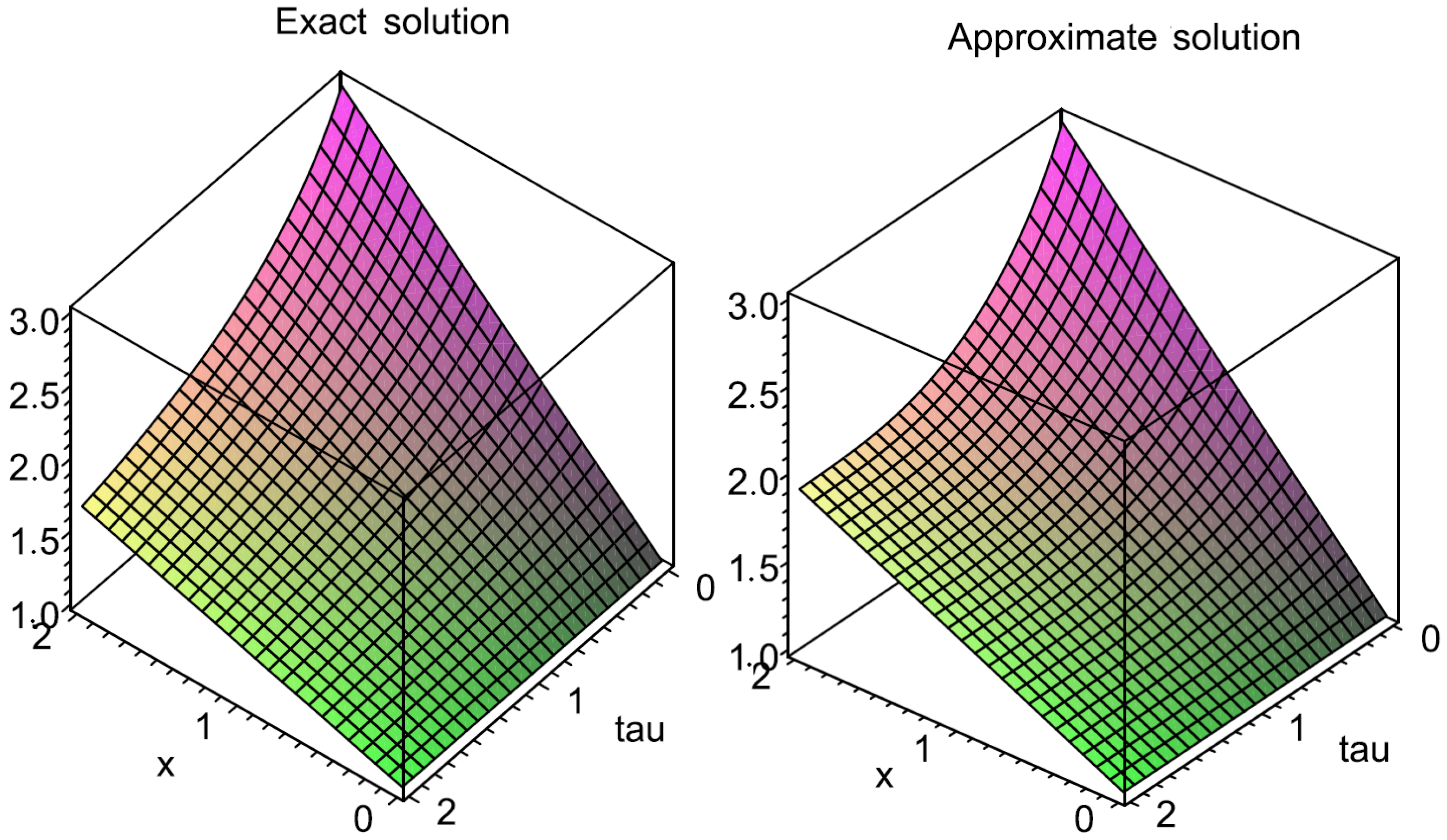
3.2. Solving the Nonlinear Fractional Partial Differential Equations

This section addresses the solution strategies for general nonlinear fractional partial differential equations, including the incorporation of initial conditions for the system

$${}_{ }{}^{c}D_{0^{+}}^{\rho }u(x,\tau )+Ru(x,\tau )+Nu(x,\tau )=g(x,\tau ),$$

(42)

where $\tau >0,x\in \mathbb{R},m-1<\rho \le m,m=1,2,\cdots$ and the initial conditions

$${\left[{\displaystyle \frac{{\partial }^{m-1}u(x,\tau )}{\partial {\tau }^{m-1}}}\right]}_{\tau =0}=h_{m-1}\left(x\right),$$

(43)

${}_{ }{}^{c}D_{\tau }^{\rho }u(x,\tau )$ is the Caputo fractional derivative of the function $u(x,\tau )$, R is the linear differential operator, N represents the general nonlinear differential operator and $g(x,\tau )$ is the source term.

Applying the Elzaki transform on both sides of (42), and using the differentiation property of this transform, we have

$$E\left[u(x,\tau )\right]=\sum _{k=0}^{m-1}{h}_k\left(x\right)v^{2+k}+v^{\rho }[E\left[g(x,\tau )\right]-E\left[Ru(x,\tau )\right]-E\left[Nu(x,\tau )\right]].$$

(44)

Taking the inverse transform on both sides of Equation (44) and then by using the initial conditions (43), we obtain

$$u(x,\tau )=G(x,\tau )-E^{-1}\left\{v^{\rho }[Ru(x,\tau )+Nu(x,\tau )]\right\}$$

(45)

where

$$G\left(\tau \right)=\sum _{k=0}^{m-1}{h}_k\left(x\right)v^{2+k}+v^{\rho }E\left[g(x,\tau )\right].$$

Now, applying the new MFTDM, we can assume that the solution can be expressed as a infinite series,

$$u(x,\tau )=\sum _{r=0}^{\infty }{u}_r(x,\tau ),$$

(46)

and then decompose the nonlinear term $Nu$ into a series   

$$Nu(x,\tau )=\sum _{r=0}^{\infty }{N}_{r}U(x,\tau ).$$

(47)

Using (46) and (47), we can rewrite (45). We obtain

$$\sum _{r=0}^{\infty }{u}_r(x,\tau )=G(x,\tau )-E^{-1}\left\{v^{\rho }[\sum _{r=0}^{\infty }R{u}_r(x,\tau )+\sum _{r=0}^{\infty }{N}_{r}U(x,\tau )]\right\}.$$

(48)

By comparing both sides of (48), the recursive relations are given by

$$\begin{array}{ccc}\hfill u_0(x,\tau )& =& G(x,\tau )\hfill \\ \hfill u_{r+1}(x,\tau )& =& -E^{-1}\left\{v^{\rho }\left[R{u}_r(x,\tau )+N_{r}U(x,\tau )\right]\right\}.\hfill \\ \hfill \end{array}$$

(49)

Finally, we approximate the solution $u(x,\tau )$ by the truncated series

$$u(x,\tau )={\Phi }_N(x,\tau )=\sum _{k=0}^N{u}_k(x,\tau ).$$

(50)

Example 3.

We consider the nonlinear time-fractional partial differential equation

$${}_{ }{}^{c}D_{0^{+}}^{\rho }u(x,\tau )+u(x,\tau )u_x(x,\tau )-u_x(x,\tau )=0,0<\rho \le 1$$

(51)

and the initial condition $u(x,0)=x+1$. If $\rho =1$, the exact solution for (51) is

$$u(x,t)=1+{\displaystyle \frac{x}{1+\tau }}=1+x\left(-\tau +{\tau }^2-{\tau }^3+{\tau }^4-{\tau }^5+{\tau }^6-{\tau }^7+{\tau }^8-{\tau }^9+\cdots \right).$$

According to the MFTDEM, we obtain

$$\begin{array}{ccc}\hfill u_0(x,\tau )& =& x+1;\hfill \\ \hfill u_{r+1}\left(\tau \right)& =& -E^{-1}\left\{v^{\rho }\left[{\left(u_r\right)}_x(x,\tau )]\right\}-E^{-1}\left\{v^{\rho }E[N_{r}U(x,\tau )\right]\right\}.\hfill \\ \hfill \end{array}$$

(52)

We use (52) to obtain

$$\begin{array}{ccc}\hfill u_0(x,\tau )& =& x+1;\hfill \\ \hfill u_1(x,\tau )& =& -x{\displaystyle \frac{{\tau }^{\rho }}{\Gamma (\rho +1)}}\hfill \\ \hfill u_2(x,\tau )& =& 2x{\displaystyle \frac{{\tau }^{2\rho }}{\Gamma (2\rho +1)}}-x{\displaystyle \frac{\Gamma (2\rho +1)}{{\Gamma }^2(\rho +1)\Gamma (3\rho +1)}}{\tau }^{3\rho };\hfill \\ \hfill u_3(x,\tau )& =& -4x{\displaystyle \frac{{\tau }^{3\rho }}{\Gamma (3\rho +1)}}+\left(2x{\displaystyle \frac{\Gamma (2\rho +1)}{{\Gamma }^2(\rho +1)\Gamma (4\rho +1)}}+4x{\displaystyle \frac{\Gamma (3\rho +1)}{\Gamma (\rho +1)\Gamma (2\rho +1)\Gamma (4\rho +1)}}\right){\tau }^{4\rho }\hfill \\ \hfill & -& \left(2x{\displaystyle \frac{\Gamma (2\rho +1)\Gamma (4\rho +1)}{{\Gamma }^3(\rho +1)\Gamma (3\rho +1)\Gamma (5\rho +1)}}+4x{\displaystyle \frac{\Gamma (4\rho +1)}{{\Gamma }^2(2\rho +1)\Gamma (5\rho +1)}}\right){\tau }^{5\rho }\hfill \\ \hfill & +& 4x{\displaystyle \frac{\Gamma (5\rho +1)}{{\Gamma }^2(\rho +1)\Gamma (3\rho +1)\Gamma (6\rho +1)}}{\tau }^{6\rho }-x{\displaystyle \frac{{\Gamma }^2(2\rho +1)\Gamma (6\rho +1)}{{\Gamma }^4(\rho +1){\Gamma }^2(3\rho +1)\Gamma (7\rho +1)}}{\tau }^{7\rho }.\hfill \\ \hfill ⋮\end{array}$$

The approximate solution is represented as

$$\begin{array}{ccc}\hfill u(x,\tau )& =& x+1-x{\displaystyle \frac{{\tau }^{\rho }}{\Gamma (\rho +1)}}+2x{\displaystyle \frac{{\tau }^{2\rho }}{\Gamma (2\rho +1)}}-\left(x{\displaystyle \frac{\Gamma (2\rho +1)}{{\Gamma }^2(\rho +1)\Gamma (3\rho +1)}}+4x{\displaystyle \frac{1}{\Gamma (3\rho +1)}}\right){\tau }^{3\rho }\hfill \\ \hfill & +& \left(2x{\displaystyle \frac{\Gamma (2\rho +1)}{{\Gamma }^2(\rho +1)\Gamma (4\rho +1)}}+4x{\displaystyle \frac{\Gamma (3\rho +1)}{\Gamma (\rho +1)\Gamma (2\rho +1)\Gamma (4\rho +1)}}\right){\tau }^{4\rho }\hfill \\ \hfill & -& \left(2x{\displaystyle \frac{\Gamma (2\rho +1)\Gamma (4\rho +1)}{{\Gamma }^3(\rho +1)\Gamma (3\rho +1)\Gamma (5\rho +1)}}+4x{\displaystyle \frac{\Gamma (4\rho +1)}{{\Gamma }^2(2\rho +1)\Gamma (5\rho +1)}}\right){\tau }^{5\rho }\hfill \\ \hfill & +& 4x{\displaystyle \frac{\Gamma (5\rho +1)}{{\Gamma }^2(\rho +1)\Gamma (3\rho +1)\Gamma (6\rho +1)}}{\tau }^{6\rho }-x{\displaystyle \frac{{\Gamma }^2(2\rho +1)\Gamma (6\rho +1)}{{\Gamma }^4(\rho +1){\Gamma }^2(3\rho +1)\Gamma (7\rho +1)}}{\tau }^{7\rho }+\cdots \hfill \end{array}$$

By taking $\rho =1,M_0=3,M=5$ and $\Delta \tau =0.4$, we find the approximate solution of the MTDETM for (51) (see Figure 3):

$$\left\{\begin{array}{c}{\Phi }_3^0\left(\tau \right)=1+x(-\tau +{\tau }^2-{\tau }^3+{\tau }^4-{\displaystyle \frac{13}{15}}{\tau }^5+{\displaystyle \frac{2}{3}}{\tau }^6-{\displaystyle \frac{29}{63}}{\tau }^7+{\displaystyle \frac{71}{252}}{\tau }^8-{\displaystyle \frac{86}{567}}{\tau }^9)+\cdots \cdots ;0\le \tau \le 0.4.\hfill \\ {\Phi }_3^1\left(\tau \right)=1+x\left(0.6960000000-0.4844160000\tau +0.3371535360{\tau }^2-0.2346588610{\tau }^3\right)+\cdots \cdots ;0.4\le \tau \le 0.8.\hfill \\ {\Phi }_3^2\left(\tau \right)=1+x\left(0.6960000000-0.4844160000\tau +0.3371535360{\tau }^2-0.2346588610{\tau }^3\right)+\cdots \cdots ;0.4\le \tau \le 0.8.\hfill \\ {\Phi }_3^3\left(\tau \right)=1+x\left(0.6960000000-0.4844160000\tau +0.3371535360{\tau }^2-0.2346588610{\tau }^3\right)+\cdots \cdots ;0.4\le \tau \le 0.8.\hfill \\ {\Phi }_3^4\left(\tau \right)=1+x\left(0.6960000000-0.4844160000\tau +0.3371535360{\tau }^2-0.2346588610{\tau }^3\right)+\cdots \cdots ;0.4\le \tau \le 0.8.\hfill \\ {\Phi }_3^5\left(\tau \right)=1+x\left(0.6960000000-0.4844160000\tau +0.3371535360{\tau }^2-0.2346588610{\tau }^3\right)+\cdots \cdots ;0.4\le \tau \le 0.8.\hfill \\ {\Phi }_3^6\left(\tau \right)=1+x\left(0.4041001262-0.1632969120\tau +0.06598830275{\tau }^2-0.02666588147{\tau }^3\right)+\cdots ;0.8\le \tau \le 1.2.\hfill \\ {\Phi }_3^7\left(\tau \right)=1+x\left(0.2570883446-0.06609441693\tau +0.01699210424{\tau }^2-0.004368471950{\tau }^3\right)+\cdots ;1.2\le \tau \le 1.6.\hfill \\ {\Phi }_3^8\left(\tau \right)=1+x\left(0.1769438033-0.03130910953\tau +0.005539952918{\tau }^2-0.0009802603394{\tau }^3\right)+\cdots ;0.8\le \tau \le 1.\hfill \end{array}\right.$$

Example 4.

We consider the nonlinear fractional partial differential equation

$${}_{ }{}^{c}D_{0^{+}}^{\rho }u(x,\tau )+{\displaystyle \frac{2}{\tau }}u(x,\tau )u_x(x,\tau )=0,x\ne 0,1<\rho \le 2$$

(53)

under the initial condition $u(x,0)=0,u_{\tau }(x,0)={\displaystyle \frac{1}{x}}$. If $\rho =2$, then exact solution for $\left(53\right)$ is

$$u(x,\tau )=tan\left({\displaystyle \frac{\tau }{x}}\right)={\displaystyle \frac{\tau }{x}}+{\displaystyle \frac{{\tau }^3}{3x^3}}+2{\displaystyle \frac{{\tau }^5}{15x^5}}+{\displaystyle \frac{17{\tau }^7}{315x^7}}+{\displaystyle \frac{62{\tau }^9}{2835x^9}}+{\displaystyle \frac{1382{\tau }^{11}}{155925x^{11}}}+{\displaystyle \frac{21844{\tau }^{13}}{6081075x^{13}}}+\cdots .$$

From formula (45), we obtain

$$\begin{array}{cc}\hfill u_0(x,\tau )& ={\displaystyle \frac{\tau }{x}}\hfill \\ \hfill u_{r+1}\left(\tau \right)& =-2E^{-1}\left\{v^{\rho }E\left[N_{r}U(x,\tau )\right]\right\}.\hfill \end{array}$$

(54)

Using formula (54), we have

$$\begin{array}{ccc}\hfill u_0(x,\tau )& =& {\displaystyle \frac{\tau }{x}}\hfill \\ \hfill u_1(x,\tau )& =& {\displaystyle \frac{2}{\Gamma (\rho +2)}}{\displaystyle \frac{{\tau }^{\rho +1}}{x^3}}\hfill \\ \hfill u_2(x,\tau )& =& {\displaystyle \frac{16}{\Gamma (2\rho +2)}}{\displaystyle \frac{{\tau }^{2\rho +1}}{x^5}}+{\displaystyle \frac{24\Gamma (2\rho +2)}{{\Gamma }^2(\rho +2)\Gamma (3\rho +2)}}{\displaystyle \frac{{\tau }^{3\rho +1}}{x^7}}\hfill \\ \hfill ⋮\end{array}$$

Therefore, the approximate solution is given as

$$\begin{array}{ccc}\hfill u(x,\tau )& =& {\displaystyle \frac{\tau }{x}}+{\displaystyle \frac{2}{\Gamma (\rho +2)}}{\displaystyle \frac{{\tau }^{\rho +1}}{x^3}}+{\displaystyle \frac{16}{\Gamma (2\rho +2)}}{\displaystyle \frac{{\tau }^{2\rho +1}}{x^5}}+{\displaystyle \frac{24\Gamma (2\rho +2)}{{\Gamma }^2(\rho +2)\Gamma (3\rho +2)}}{\displaystyle \frac{{\tau }^{3\rho +1}}{x^7}}+\cdots \hfill \\ \hfill \end{array}$$

By taking $\rho =2,M_0=3$ and $M=1$, we obtain the approximate solution of the MTDETM for (53) (see Figure 4):

$$u(x,\tau )={\displaystyle \frac{\tau }{x}}+{\displaystyle \frac{{\tau }^3}{3x^3}}+{\displaystyle \frac{2{\tau }^5}{15x^5}}+{\displaystyle \frac{17{\tau }^7}{315x^7}}+{\displaystyle \frac{62{\tau }^9}{2835x^9}}+{\displaystyle \frac{1142{\tau }^{11}}{155925x^{11}}}+{\displaystyle \frac{13324{\tau }^{13}}{6081075x^{13}}}+\cdots ;0\le \tau \le {\tau }_i.$$

4. Program of the MFTDM

In this part, we propose a computer program of the MFTDM to solve fractional order differential equations. As soon as the user specifies the function f and the value of $\alpha$, the number of iterations n and the initial condition $U\left[i\right]$ are shown, taking the interval $[0,T]$ and $N-1$ as the number of subintervals and choosing the same length $\Delta t$. Also, we propose it in the Maple computer algebra language. The program (Algorithm 1) is as follows:

Algorithm 1: Programme of the novel algorithm.

Programme: $>abc:=\mathbf{proc}\left(m\right)$        $g:=t\to t^i{\displaystyle \frac{U\left[i\right]}{i!}}$;        $eval\left(sum\right(g\left(t\right),i=0..m-1\left)\right)$        endproc: Warning, ’g’ is implicitly declared local to procedure ’abc’ $>u[0,0]:=t\to abc\left(m\right):$ $>u[0,1]:=unapply(1/GAMMA\left(\alpha \right)\ast int({(t-s)}^{(\alpha -1)}\ast f(s,u[0,0]\left(s\right)),s=0\dots t),t);$ >for k from 2 to n do $u[0,k]:=unapply(1/GAMMA\left(\alpha \right).int({(t-s)}^{(\alpha -1)}\ast (f(s,sum(u[0,j]\left(s\right),j=0\dots k-1))-f(s,sum(u[0,j]\left(s\right),j=0\dots k-2))),s=0..t),t)$; end; $>\Phi [0,k]:=simplify\left(unapply\right(sum\left(u\right[0,j\left]\right(t),j=0..n),t\left)\right);$ >for i from 1 to $N-1$ do $t\left[i\right]:=i\Delta t:$ $u[i,0]:=unapply(\Phi [i-1,n\left]\right(t\left[i\right],t);$ $u[i,1]:=unapply(1/GAMMA\left(\alpha \right)\ast int({(t-s)}^{(\alpha -1)}\ast f(s,u[i,0]\left(s\right)),s=t\left[i\right]..t),t);$ >for k from 2 to n do $u[i,k]:=unapply(1/GAMMA\left(\alpha \right).int({(t-s)}^{(\alpha -1)}\ast (f(s,sum(u[i,j]\left(s\right),j=0\dots k-1))-f(s,sum(u[i,j]\left(s\right),j=0\dots k-2))),s=t\left[i\right]..t),t)$; print $u[i,k]$ end; $>\Phi [i,k]:=simplify\left(unapply\right(sum\left(u\right[i,j\left]\right(t),j=0..n),t\left)\right).$

5. Conclusions

This study introduces the multistage fractional telescoping decomposition Elzaki method (MFTDEM) as a powerful and efficient approach to solving nonlinear fractional initial value problems. By combining the multistage telescoping decomposition technique with the Elzaki transform, the method provides a solution in the form of a rapidly converging series, accurately approximating the exact solution. The numerical experiments presented confirm the method’s high precision, demonstrating its potential to solve a broad range of complex problems in various scientific and engineering fields with minimal computational effort.

The proposed MFTDEM offers a versatile tool for addressing nonlinear fractional differential equations, contributing significantly to the ongoing development of numerical methods in fractional calculus. Future research may explore the extension of this method to more complex systems and higher-dimensional problems.

References

1. Adomian, G. Solution of physical problems by decomposition. Comp. Math. Appl. 1994, 27, 145–154. [Google Scholar] [CrossRef]
2. Momani, S.; Shawagfeh, N. Decomposition method for solving fractional Riccati differential equations. Asian J. Math. Comput. 2016, 13, 203–214. [Google Scholar] [CrossRef]
3. Elzaki, T.M.; Chamekh, M. Solving nonlinear fractional differential equations using a new decomposition method. Univ. J. Appl. Math. Comput. 2018, 6, 27–35. [Google Scholar]
4. Ziane, D.; Belghaba, K.; Cherif, M.H. Fractional homotopy perturbation transform method for solving the time-fractional KdV, k(2,2) and Burgers equations. Int. J. Open Prob. Comput. Sci. Math. 2015, 8, 63–75. [Google Scholar] [CrossRef]
5. He, J.H. A coupling method of homotoping technique and perturbation technique for nonlinear problems. Int. J. Nonlinear Mech. 2000, 35, 37–43. [Google Scholar] [CrossRef]
6. Hilall, E.; Elzaki, M.T. Solution of nonlinear partial differential equations by new Laplace variational iteration method. J. Funct. Spaces 2014, 2014, 790714. [Google Scholar] [CrossRef]
7. Afshan, K.; Tauseef, M.S. Coupling of Laplace transform and correction functional for wave equations. Word J. Mod. Simul. 2013, 9, 173–180. [Google Scholar]
8. Elzaki, T.M.; Elzaki, S.M. On the connections between Laplace and Elzaki transforms. Adv. Theor. Appl. Math. 2014, 6, 1–10. [Google Scholar]
9. Abel-Rady, A.S.; Rida, S.Z.; Arafa, A.A.M.; Abedi-Rahim, H.R. Variational iteration Sumudu transform method for solving fractional nonlinear gaz dynamics equation. Int. J. Res. Stud. Sci. Eng. Technol. 2014, 1, 82–90. [Google Scholar]
10. Kumar, D.; Singh, J.; Rathore, S. Sumudu decomposition method for nonlinear equations. Int. Math. Forum 2012, 7, 515–521. [Google Scholar]
11. Singh, J.; Kumar, D.; Sushila. Homotopy perturbation Sumudu transform method for nonlinear equations. Adv. Theor. Appl. Mach. 2011, 4, 165–175. [Google Scholar]
12. Rathore, S.; Kumar, D.; Singh, J.; Gupta, S. Homotopy analysis Sumudu transform method for nonlinear equations. Int. J. Ind. Math. 2012, 4, 301–314. [Google Scholar]
13. Elzaki, T.M. The new integral transform Elzaki transform. Glob. J. Pure Appl. Math. 2011, 7, 57–64. [Google Scholar]
14. Elzaki, T.M.; Hilal, E.M.A. Homotopy perturbation and Elzaki transform for solving nonlinear partial differential equations. Math. Theor. Mod. 2012, 2, 33–42. [Google Scholar]
15. Elzaki, T.M.; Elzaki, S.M.; Elnour, E.A. On the new integral transform “Elzaki Transform” fundamental properties investigations and applications. Glob. J. Math. Sci. 2012, 2, 1–13. [Google Scholar]
16. Elzaki, T.M. On the Elzaki transform and ordinary differential equation with variable coefficients. Adv. Theor. Appl. Math. 2011, 6, 13–18. [Google Scholar]
17. Elzaki, T.M.; Biazar, J. Homotopy perturbation method and Elzaki transform for solving system of nonlinear partial differential equatios. World Appl. Sci. 2013, 24, 944–948. [Google Scholar]
18. Riabi, L.; Belghaba, K.; Cherif, M.H.; Ziane, D. Homotopy perturbation method combined with ZZ transform to solve some nonlinear fractional differential equations. Int. J. Anal. Appl. 2019, 17, 406–419. [Google Scholar]
19. Al-Refai, M.; Abu-Dalu, M.; Al-Rawashde, A. Telescoping decomposition method for solving first order nonlinear differential equations. In Proceedings of the International Multi-Conference of Engineers and Computer Scientists, (IMECS 2008), Kowloon, Hong Kong, 19–21 March 2008. [Google Scholar]
20. Khalid, M.; Sultana, M.; Zaidi, F.; Arshad, U. An Elzaki transform decomposition algorithm applied to a class of non-linear differential equations. J. Nat. Sci. Res. 2015, 5, 48–55. [Google Scholar]
21. Nibron, M.; Mishra, A.K.; Kabala, D. Telescoping decomposition method for solving second order nonlinear differential equations. Int. J. Eng. Res. Technol. 2014, 3, 590–595. [Google Scholar]
22. Ige, O.E.; Heilio, M.; Oderinu, R.A.; Elzaki, T.M. Adomian polynomial and Elzaki transform method of solving third order Korteweg-De Vries equatios. Glob. J. Pure Appl. Math. 2019, 15, 261–277. [Google Scholar]
23. Ige, O.E.; Oderinu, R.A.; Elzaki, T.M. Adomian polynomial and Elzaki transform method for solving Klein Gordon equations. Int. J. Appl. Math. 2019, 32, 451–468. [Google Scholar] [CrossRef]
24. Saadeh, R.; Qazza, A.; Burqan, A. A new integral transform: ARA transform and its properties and applications. Symmetry 2020, 12, 925. [Google Scholar] [CrossRef]
25. Zafar, Z.U.A. ZZ transform method. Int. J. Adv. Eng. Glob. Technol. 2016, 4, 1605–1611. [Google Scholar]
26. Zafar, Z.U.A. Application of ZZ transform method on some fractional differential equation. Int. J. Adv. Eng. Glob. Technol. 2016, 4, 1355–1363. [Google Scholar]
27. Ziane, D. The combined of Homotopy analysis method with new transform for nonlinear partial differential equations. Malaya J. Math. 2018, 6, 34–40. [Google Scholar] [CrossRef]
28. Raghavendar, K.; Pavani, K.; Aruna, K.; Okposo, N.I.; Inc, M. Application of Natural Transform Decomposition Method for Solution of Fractional Richards Equation. Contemp. Math. 2024, 5, 5881. [Google Scholar] [CrossRef]
29. Kharrat, B.N. New Double Kharrat-Toma Transform and its Application in Partials Differential Equations. World Appl. Sci. J. 2024, 42, 30–36. [Google Scholar]
30. Bouhassoun, A. Multistage telescoping decomposition method for solving fractional differential equations. Int. J. Appl. Math. 2013, 43, 1–7. [Google Scholar]
31. Chita, F.; Belghaba, K. Solving systems of nonlinear fractional differential equations using multistage telescoping decomposition method. Asian J. Math. Comput. 2016, 13, 203–214. [Google Scholar]
32. Diethelm, K. The Analysis Fractional Differential Equations; Springer: Berlin/Heidelberg, Germany, 2010. [Google Scholar]
Figure 1. The left image shows a graph of the exact solution and approximate solutions of Equation (26) for ρ = 1 . The right image shows a graph of the approximate solutions of (26) for different values of ρ .
Fractalfract 09 00065 g001
Figure 2. The left image shows a graph of the exact solution and approximate solutions of Equation (36) for ρ = 1 . The right image shows a graph of the approximate solutions of (36) for different values of ρ .
Fractalfract 09 00065 g002
Figure 3. The right image shows a graph of the exact solution. The left image shows a graph of the approximate solutions of (51) for ρ = 1 .
Fractalfract 09 00065 g003
Figure 4. The right image shows a graph of the exact solution. The left image shows a graph of the approximate solutions of (53) for ρ = 1 .
Fractalfract 09 00065 g004