Abstract
This manuscript aims to establish the existence, uniqueness, and stability of solutions for Langevin fractional differential equations involving the generalized Liouville-Caputo derivative. Using a novel approach, we derive existence and uniqueness results through fixed-point theorems, extending and generalizing several existing findings in the literature. To demonstrate the applicability of our results, we provide a practical example that validates the theoretical framework.
1. Introduction
In fractional calculus, the concept of integer order has been generalized to include arbitrary orders. Fractional-order models are generally more appropriate and accurate than integer-order models, as they provide a better representation of genetic processes and memory. In recent decades, fractional calculus has attracted considerable interest due to its extensive applications across diverse scientific disciplines. It has been utilized in various fields, such as biology, polymer science, heat conduction, signal processing, nonlinear earthquake oscillations, capacitor theory, image processing, groundwater problems, blood flow dynamics, electrical circuits, biophysics, viscoelasticity, and more. For additional applications of fractional differential equations, please refer to the references cited in [1,2,3,4].
The classical form of the Langevin equation was first presented by Paul Langevin in 1908 [5]. It was the first equation to describe the Brownian motion of particles [5]. However, some areas of fractal disorder were not adequately addressed by the classical Langevin equation. In mathematical physics, this is important for systems such as fractional reaction–diffusion [6,7], harmonic oscillators, noise sources with correlations [8], and the nature of quantum noise [9,10], among others. When there is no macroscopic system and the differential equation for the microscopic time scale is invalid, the fractional Langevin equation (LE) is more useful than the usual LE; see, for instance [11]. The Langevin equation and fractional dynamics are referenced in [12]. The Langevin equation, which has applications in stochastic problems in physics, chemistry, and electrical engineering, is seen in [13] .
Therefore, researchers aim to generalize fractional operators to better capture the hidden aspects of real non-local phenomena. Meanwhile, many researchers focus on fractional integrals and derivatives with non-local and non-singular kernels [14,15,16]. One of the emerging trends in fractional calculus is the study of discrete fractional operators, which have been shown to have valuable applications in various fields [17,18]. The authors of [19] introduced the Caputo version of generalized fractional derivatives. From a mathematical perspective, it is essential to consider fractional derivatives of functions belonging to specific function spaces. Additionally, the authors in [20] generalized the Liouville–Caputo fractional derivatives and their Caputo modification.
The existence and stability of solutions for fractional differential equations of different orders have been the focus of recent research. We now review several notable and contemporary papers on existence and uniqueness results for various types of fractional differential equations, as discussed in [21,22,23,24]. Hyers–Ulam (H-U) stability was initially introduced by Ulam in 1940 [25,26] and can be used to address the difference between approximate and exact solutions. Many researchers have conducted further studies on the stability of fractional equation solutions using this method. For example, see [27,28,29,30].
In [31], we consider a nonlinear fractional Langevin equation involving two fractional orders with given initial conditions.
where , , , and . In [32], the study investigates the existence of extremal solutions for the fractional Langevin equation involving nonlinear boundary conditions.
where is the Caputo fractional derivative of order .
In [33], the study examines the existence and uniqueness of solutions for the anti-periodic boundary value problem of a Langevin equation with two different fractional orders.
where is a real number, denotes the Caputo fractional derivative of order , and is a continuous function.
In [34], the existence and uniqueness of solutions with periodic boundary conditions for the fractional Langevin equation using the generalized Caputo derivative are investigated.
where and represent the generalized Caputo fractional derivative operators of orders , .
We develop and investigate a new version of the Langevin equation that utilizes generalized Liouville–Caputo derivatives, inspired by previous work. We examine the existence, uniqueness, and stability of the solution to the problem:
where the Liouville-Caputo-type generalized fractional derivatives of orders , , and are represented by the expressions and , respectively. The generalized fractional integral operator of order and is denoted by , and the given continuous function is .
Preliminaries
The aims of this section, we recall some basic definitions and results that are required for latter.
The Banach space of all continuous functions is denoted by . The norm is defined as
Let . The Banach space has a norm which is defined as follows:
To begin, let us define the order of fractional derivatives in the following way:
Definition 1
([35]). For , the generalized left-sided fractional integral of order and for is defined as follows:
Definition 2
([36]). The generalized fractional derivatives are defined for , , , and in terms of the generalized fractional integrals, as defined below:
Definition 3
([20]). Assume and for . The generalized fractional derivatives of the Liouville–Caputo type, denoted by , are defined as follows:
Lemma 1
([20]). The definitions of the left generalized Liouville–Caputo derivatives for and are as follows:
Lemma 2
([20]). Let or and . Then:
Specifically, for , we have the following:
In Figure 1 and Figure 2, the dynamical behavior of the generalized Liouville–Caputo derivatives can be observed in the given functions , , respectively.
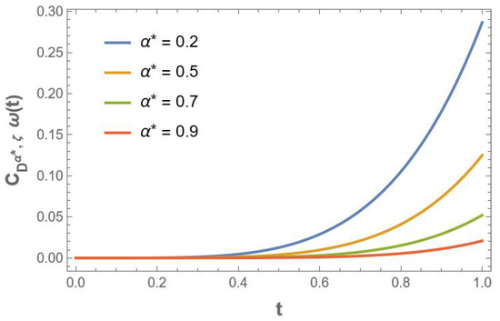
Figure 1.
.
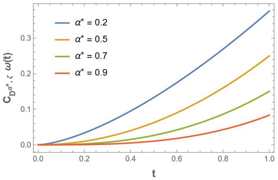
Figure 2.
.
Theorem 1
(Banach FPT [37]). Let be a non-empty subset of a Banach space . If is a contraction mapping, then has a unique fixed point.
Theorem 2
(Schauder’s FPT [38]). Let be a non-empty, closed, convex subset of a Banach space . The operator has at least one fixed point if is a compact operator.
2. Main Results
The purpose of this section is to discuss the existence and uniqueness of solutions for problem (3).
Lemma 3.
Let , then the boundary value problem
has a solution is given by
where
Proof.
Applying Lemma 2 and the operator to the fractional differential equation in Equation (9) yields the following:
for some .
The general solution of the Equation (9) is determined by applying to both sides of Equation (11).
where .
We deduce that by applying the constraint in Equation (12). After substituting into Equation (12) and modifying the resulting equation using the operator , we obtain the following:
with the help of Equations (12) and (13) and the boundary conditions and , one can solve the algebraic system of equations for and .
and
The result in Equation (10) can be obtained by substituting the values of , , and into Equation (12). The proof is now complete. □
We demonstrate that the operator possesses a fixed point, which serves as the solution to problem (3). We define operator by the following:
We introduce the following hypothesis, which is required for the subsequent results.
- Let be a continuous function.
- For every and , there is a constant .
For simplicity, we denote
where
We discuss the uniqueness results of problem (5) using the Banach fixed point theorem.
Theorem 3.
Assume that conditions – are satisfied. Then, problem (5) has a unique solution if
Proof.
Let us define the operator as shown in Equation (14). We show that is a contraction. Define the set
Then, clearly, is bounded. For , we have the following:
Therefore, we have
The operator is a contraction since , as shown in (15). Therefore, the operator has a unique fixed point according to Theorem 1. Consequently, problem (5) has a unique solution. The proof is complete. □
The solution of problem (5) exists if the operator satisfies the Schauder fixed point theorem.
We present the following hypothesis.
- For any , there exists a continuous function such that
Theorem 4.
Let – be satisfied. If , then problem (5) has at least one solution.
Proof.
Consider the set
It is clear that the subset is evidently convex, closed, and bounded. We will show that meets the requirements specified in Theorem 2. The proof will be divided into three steps.
Step 1: We demonstrate that . For all and , we obtain the following:
This implies that . Thus, the operator maps into itself.
Step 2: Next, we will show that is a continuous function. Let be a sequence such that . We have the following:
Thus, by the Lebesgue dominated convergence theorem, . Hence, is continuous.
Step 3: This clearly shows the uniform boundedness of the operator . Now, we present the equicontinuity of . For this, we suppose such that . We have
This implies that as , independently of . Thus, is equicontinuous, which implies that is relatively compact on . Consequently, by the Arzelà–Ascoli theorem, we deduce that is compact on . The proof is complete because Theorem 2 guarantees that problem (5) has at least one solution. □
3. Stability
In this section, we study the stability of problem (5).
Assume . Next, we examine the following inequality:
Definition 4.
If there exists such that for every and for each solution of inequality (16), there exists a solution of problem (5), then problem (5) is said to be H-U stable such that
Definition 5.
If there exists a function such that , and for each and every solution of the inequality (16), there exists a unique solution of (5), then problem (5) has generalized H-U stability.
Remark 1.
A function is a solution of the inequality (16) if and only if there exists a function (which depends on solution ð) such that
- ,
Lemma 4.
The solution of the given problem
is
Theorem 5.
Let – hold. Then the problem (5) is H-U stable on and consequently generalized H-U stable.
Proof.
Let . Suppose is a solution that satisfies inequality (16), which is defined by (10), and let be its unique solution. Applying Remark 1, for every , we have the following:
Therefore, we obtain
If we let
then, the H-U stability condition is satisfied.
More generally,
the generalized H-U stability condition is also fulfilled. □
4. Illustrative Examples
In this section, we present examples to demonstrate the applicability of the analytical findings.
4.1. Example
Consider the following problem:
Clearly, is a continuous function. Therefore, we have the following:
Here, , , , , , , a = 1, , , = 2.
Now
Therefore, assumption is met with the value of . Using the given date, we find , , , .
Problem (19) has a unique solution because all the conditions of Theorem 3 are satisfied. Additionally, we , where .
As a consequence, problem (19) has at least one solution since each of the conditions of Theorem 4 is satisfied. Additionally, the Theorem 5 and problem (19) are both stable for Hyers–Ulam and generalized Hyers–Ulam. See the Figure 3 for more understanding.
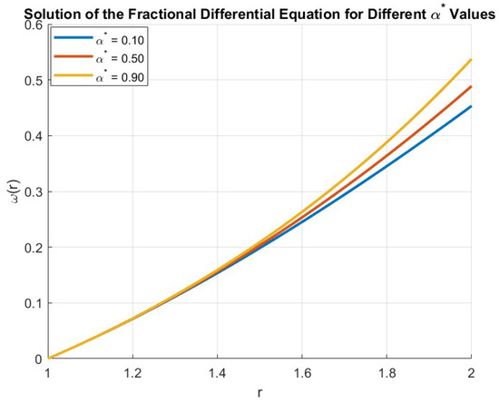
Figure 3.
Graph represents the dynamical behavior of the solutions to the fractional differential equation.
4.2. Example
Consider the following problem:
Clearly, is a continuous function. Therefore, we have the following:
Here, , , , , , , a = 2, , , = 3.
Now
Therefore, assumption is met with the value of . Using the given date, we find , , , .
Problem (20) has a unique solution because all the conditions of Theorem 3 are satisfied. Additionally, we , where .
As a consequence, problem (20) has at least one solution since each of the conditions of Theorem 4 is satisfied. Additionally, the Theorem 5 and problem (20) are both stable for Hyers-Ulam and generalized Hyers-Ulam.
5. Conclusions and Future Goals
We investigated the existence, uniqueness, and stability of solutions to a fractional differential equation involving generalized Liouville–Caputo fractional derivatives. By applying the fixed-point theorem, we established these results. Additionally, we provide an example to illustrate the reliability of our findings. This paper offers a novel and valuable contribution to the literature on fractional differential equations. In future work, the given fractional boundary value problem could be extended to include other fractional derivatives, such as the ABC fractional derivative and the mABC fractional derivative.
Author Contributions
Methodology, R.U.K.; Validation, G.A.; Formal analysis, I.-L.P.; Writing—original draft, R.U.K.; writing—review and editing, R.U.K.; Supervision, M.S. All authors have read and agreed to the published version of the manuscript.
Funding
This research received no external funding.
Data Availability Statement
As no data were used in this study, no data availability statement is applicable.
Conflicts of Interest
The authors declare no conflicts of interest.
References
- Kilbas, A.A.; Srivastava, H.M.; Trujillo, J.J. Theory and Applications of Fractional Differential Equations; Elsevier: Amsterdam, The Netherlands, 2006; Volume 204. [Google Scholar]
- Podlubny, I. Fractional differential equations, to methods of their solution and some of their applications. In Fractional Differential Equations: An Introduction to Fractional Derivatives; Elsevier: Amsterdam, The Netherlands, 1998; Volume 340. [Google Scholar]
- Khan, H.; Ahmed, S.; Alzabut, J.; Azar, A.T. A generalized coupled system of fractional differential equations with application to finite time sliding mode control for Leukemia therapy. Chaos Solitons Fractals 2023, 174, 113901. [Google Scholar] [CrossRef]
- Magin, R.L. Fractional Calculus in Bioengineering Begell; House Publishers Inc.: Danbury, CT, USA, 2006. [Google Scholar]
- Lemons, D.S.; Gythiel, A.A. Paul Langevin’s 1908 paper “On the Theory of Brownian Motion” [“Sur la thiorie du mouvement brownien”, CR Acad. Sci. (Paris) 146, 530–533 (1908)]. Am. J. Phys. 1997, 65, 1079–1081. [Google Scholar] [CrossRef]
- Datsko, B.; Gafiychuk, V. Complex nonlinear dynamics in subdiffusive activator-inhibitor systems. Commun. Nonlinear Sci. Numer. Simul. 2012, 17, 1673–1680. [Google Scholar] [CrossRef]
- Datsko, B.; Gafiychuk, V. Complex spatio-temporal solutions in fractional reaction-diffusion systems near a bifurcation point. Fract. Calc. Appl. Anal. 2018, 21, 237–253. [Google Scholar] [CrossRef]
- Hohenberg, P.C.; Halperin, B.I. Theory of dynamic critical phenomena. Rev. Mod. Phys. 1977, 49, 435. [Google Scholar] [CrossRef]
- Vinales, A.D.; Desposito, M.A. Anomalous diffusion: Exact solution of the generalized Langevin equation for harmonically bounded particle. Phys. Rev. E-Stat. Nonlinear Soft Matter Phys. 2006, 73, 016111. [Google Scholar] [CrossRef] [PubMed]
- Metiu, H.; Schon, G. Description of Quantum noise by a Langevin equation. Phys. Rev. Lett. 1984, 53, 13. [Google Scholar] [CrossRef]
- West, B.J.; Picozzi, S. Fractional Langevin model of memory in financial time series. Phys. Rev. E 2002, 65, 037106. [Google Scholar] [CrossRef] [PubMed]
- Ślęzak, J. Langevin equation and fractional dynamics. arXiv 2018, arXiv:1810.02412. [Google Scholar]
- Coffey, W.; Kalmykov, Y.P. The Langevin equation: With applications to stochastic problems in physics, chemistry and electrical engineering. In World Scientific Series in Contemporary Chemical Physics; World Scientific: Singapore, 2012; Volume 27. [Google Scholar]
- Caputo, M.; Fabrizio, M. A new definition of fractional derivative without singular kernel. Prog. Fract. Differ. Appl. 2015, 1, 73–85. [Google Scholar]
- Gao, F.; Yang, X.J. Fractional Maxwell fluid with fractional derivative without singular kernel. Therm. Sci. 2016, 20 (Suppl. S3), 871–877. [Google Scholar] [CrossRef]
- Losada, J.; Nieto, J.J. Properties of a new fractional derivative without singular kernel. Prog. Fract. Differ. Appl. 2015, 1, 87–92. [Google Scholar]
- Atıcı, F.M.; Şengül, S. Modeling with fractional difference equations. J. Math. Anal. Appl. 2010, 369, 1–9. [Google Scholar] [CrossRef]
- Goodrich, C.; Peterson, A.C. Discrete Fractional Calculus; Springer: Cham, Switzerland, 2015; Volume 10, pp. 978–983. [Google Scholar]
- Almeida, R.; Malinowska, A.B.; Odzijewicz, T. Fractional differential equations with dependence on the Caputo–Katugampola derivative. J. Comput. Nonlinear Dyn. 2016, 11, 061017. [Google Scholar] [CrossRef]
- Jarad, F.; Abdeljawad, T.; Baleanu, D. On the generalized fractional derivatives and their Caputo modification. J. Nonlinear Sci. Appl. 2017, 10, 2607–2619. [Google Scholar] [CrossRef]
- Saha, K.K.; Sukavanam, N.; Pan, S. Existence and uniqueness of solutions to fractional differential equations with fractional boundary conditions. Alex. Eng. J. 2023, 72, 147–155. [Google Scholar] [CrossRef]
- Khatun, M.A.; Arefin, M.A.; Akbar, M.A.; Uddin, M.H. Existence and uniqueness solution analysis of time-fractional unstable nonlinear Schrödinger equation. Results Phys. 2024, 57, 107363. [Google Scholar] [CrossRef]
- Hatime, N.; Melliani, S.; El Mfadel, A.; Elomari, M. Existence, uniqueness, and finite-time stability of solutions for ψ-Caputo fractional differential equations with time delay. Comput. Methods Differ. Equ. 2023, 11, 785–802. [Google Scholar]
- Khan, A.U.; Khan, R.U.; Ali, G.; Aljawi, S. The study of nonlinear fractional boundary value problems involving the p-Laplacian operator. Phys. Scr. 2024, 99, 085221. [Google Scholar] [CrossRef]
- Ulam, S.M. A Collection of the Mathematical Problems; Interscience Publisheres: New York, NY, USA, 1960. [Google Scholar]
- Hyers, D.H. On the stability of the linear functional equation. Proc. Natl. Acad. Sci. USA 1941, 27, 222–224. [Google Scholar] [CrossRef] [PubMed]
- Mahdy, A.M. Stability, existence, and uniqueness for solving fractional glioblastoma multiforme using a Caputo-Fabrizio derivative. Math. Methods Appl. Sci. 2023. [Google Scholar] [CrossRef]
- Almalahi, M.A.; Abdo, M.S.; Panchal, S.K. Existence and Ulam-Hyers stability results of a coupled system of Ψ-Hilfer sequential fractional differential equations. Results Appl. Math. 2021, 10, 100142. [Google Scholar] [CrossRef]
- Ali, G.; Khan, R.U.; Kamran; Aloqaily, A.; Mlaiki, N. On qualitative analysis of a fractional hybrid Langevin differential equation with novel boundary conditions. Bound. Value Probl. 2024, 2024, 62. [Google Scholar] [CrossRef]
- Li, G.; Zhang, Y.; Guan, Y.; Li, W. Stability analysis of multi-point boundary conditions for fractional differential equation with non-instantaneous integral impulse. Math. Biosci. Eng. 2023, 20, 7020–7041. [Google Scholar] [CrossRef] [PubMed]
- Fazli, H.; Sun, H.; Nieto, J.J. Fractional Langevin equation involving two fractional orders: Existence and uniqueness revisited. Mathematics 2020, 8, 743. [Google Scholar] [CrossRef]
- Fazli, H.; Sun, H.; Aghchi, S. Existence of extremal solutions of fractional Langevin equation involving nonlinear boundary conditions. Int. J. Comput. Math. 2021, 98, 1–10. [Google Scholar] [CrossRef]
- Fazli, H.; Nieto, J.J. Fractional Langevin equation with anti-periodic boundary conditions. Chaos Solitons Fractals 2018, 114, 332–337. [Google Scholar] [CrossRef]
- Devi, A.; Kumar, A. Existence of solutions for fractional Langevin equation involving generalized Caputo derivative with periodic boundary conditions. Aip Conf. Proc. 2020, 2214, 020026. [Google Scholar]
- Katugampola, U.N. New approach to a generalized fractional integral. Appl. Math. Comput. 2011, 218, 860–865. [Google Scholar] [CrossRef]
- Katugampola, U.N. A new approach to generalized fractional derivatives. arXiv 2011, arXiv:1106.0965. [Google Scholar]
- Agarwal, R.P.; Meehan, M.; O’regan, D. Fixed Point Theory and Applications; Cambridge University Press: Cambridge, UK, 2001; Volume 141. [Google Scholar]
- Schauder, J. Der fixpunktsatz in funktionalraümen. Stud. Math. 1930, 2, 171–180. [Google Scholar] [CrossRef]
Disclaimer/Publisher’s Note: The statements, opinions and data contained in all publications are solely those of the individual author(s) and contributor(s) and not of MDPI and/or the editor(s). MDPI and/or the editor(s) disclaim responsibility for any injury to people or property resulting from any ideas, methods, instructions or products referred to in the content. |
© 2025 by the authors. Licensee MDPI, Basel, Switzerland. This article is an open access article distributed under the terms and conditions of the Creative Commons Attribution (CC BY) license (https://creativecommons.org/licenses/by/4.0/).