Solving the Fractional Allen–Cahn Equation and the Fractional Cahn–Hilliard Equation with the Fractional Physics-Informed Neural Networks

Abstract

In this paper, we present a computational framework based on fractional Physics-Informed Neural Networks combined with the $L1$ approximation of the Caputo fractional derivative to solve the fractional Allen–Cahn and fractional Cahn–Hilliard equations. Considering the limitation of the original fractional Physics-Informed Neural Networks in achieving high accuracy when applied to these highly stiff fractional equations, we propose three improved optimization strategies: adaptive non-uniform sampling, adaptive exponential moving average ratio loss weighting, and two–stage adaptive quasi optimization. By combining these strategies, three improved fPINNs algorithms are developed: f–A–PINNs, f–A–A–PINNs, and f–A–T–PINNs. Numerical experiments demonstrate that the f–A–T–PINNs algorithm achieves superior computational accuracy and improved parameter stability compared to the other algorithms.

1. Introduction

Modeling complex physical systems often involves characteristics such as nonlocality, memory effects, and power–law dynamics, where traditional integer-order differential equations exhibit inherent limitations. Fractional Partial Differential Equations (fPDEs), by introducing non-integer-order derivative operators, naturally capture the system’s long-range temporal memory and spatial nonlocality and have thus found broad applications across various scientific and engineering domains.

Solving fPDE has greater challenges compared to their integer-order counterparts, primarily due to the high computational complexity and numerical instability arising from their nonlocal operators. These issues have, to some extent, hindered the broader application and dissemination of fPDEs across various domains. Although traditional Physics-Informed Neural Networks (PINNs) [1,2] have demonstrated strong expressive power in function approximation, their efficacy relies on the classical chain rule, which holds efficiently during forward and backward propagation in neural networks but is no longer valid in the context of fractional calculus. This necessitates the development of novel Physics-Informed Neural Network Architectures specifically tailored for fPDEs. Pang et al. [3] first extended the PINNs framework to the solution of fPDEs by proposing fractional Physics-Informed Neural Networks (fPINNs). This approach employs the Grüwald–Letnikov discretization and has successfully solved both forward and inverse problems of convection–diffusion equations. As an inherently data-driven method, fPINNs do not rely on fixed meshes or discrete nodes, thus offering flexibility in handling complex geometrical domains. In contrast to the extensive research on PINNs, efforts dedicated to improving and extending fPINNs remain relatively limited. Zhang et al. [4] proposed an Adaptive Weighted Auxiliary Output fPINN (AWAO–fPINNs), which enhances training stability by introducing auxiliary variables and a dynamic weighting mechanism. Yan et al. [5] introduced a Laplace transform-based fPINNs (Laplace fPINNs), which avoids the need for a large number of auxiliary points required in conventional methods and simplifies the construction of the loss function. Furthermore, Guo et al. [6] developed Monte Carlo fPINNs (MC fPINNs) that employ a Monte Carlo sampling strategy to provide unbiased estimation of fractional derivatives from the outputs of deep neural networks, which are then used to construct soft penalty terms in the physical constraint loss, thereby reducing numerical bias.

In this paper, we investigate a framework based on fPINNs, focusing on the fractional Allen–Cahn (f–AC) equation and fractional Cahn–Hilliard (f–CH) equation. For the given Ginzburg–Laudau energy functional,

$$\mathcal{F}={\int }_{\mathsf{\Omega }}{\displaystyle \frac{{ϵ}^2}{2}}{|\nabla u|}^2+{\displaystyle \frac{\gamma }{4}}(u^2-1)dx.$$

(1)

If we take the $L^2$ gradient flow and choose the Caputo fractional derivative as the time derivative ${}_0{}^{C}D_t^{\alpha }u(x,t)(0<\alpha <1)$, we obtain the f–AC equation

$${}_0{}^{C}D_t^{\alpha }u(x,t)={ϵ}^2\mathsf{\Delta }u-\gamma (u^3-u).$$

(2)

If we take the $H^{-1}$ gradient flow, the corresponding f–CH equation can be obtained as follows:

$${}_0{}^{C}D_t^{\alpha }u(x,t)=\mathsf{\Delta }(-{ϵ}^2\mathsf{\Delta }u+\gamma (u^3-u)),$$

(3)

where $u(x,t)$ is the phase variable, and $ϵ>0$ is the interface width parameter. In addition, many consistent conditions (such as periodic boundary conditions and homogeneous Neumann boundary conditions) and initial functions should be proposed to close the system. The f–AC and f–CH equations extend their classical counterparts by replacing the time derivative with a fractional-order derivative (e.g., the Caputo derivative). This enables the effective characterization of nonlocal dynamical behaviors such as “memory effects” and “long-range interactions” in the system [7].

In the numerical solution of the f–AC equation, a variety of high-accuracy and stable discretization methods have been proposed, including the $L1$ and $L2-1_{\sigma }$ time-stepping scheme, convolution quadrature, finite element method, and spectral method. Du and Yang [7] systematically analyzed the well-posedness and maximum principle of Equation (2), and proposed a time discretization scheme such as weighted convex splitting, for which they established unconditional stability and convergence. Liao and Tang [8] developed a variable-step Crank–Nicolson-type scheme that preserves energy stability and the maximum principle within the Riemann–Liouville derivative framework, and they first established a discrete transformation relationship between Caputo and Riemann–Liouville fractional derivatives. Zhang and Gao [9] constructed a high-order finite difference scheme using the shifted fractional trapezoidal rule, which exhibits energy dissipation and maximum principle preservation.

For the f–CH equation, the numerical solution poses significantly greater challenges compared to the f–AC equation, due to the coupling of its fourth-order spatial derivative with the fractional-order temporal derivative. Liu et al. [10] proposed an efficient algorithm combining finite differences with the Fourier spectral method, effectively mitigating the high memory consumption and computational complexity caused by the nonlocality of the fractional operator. They further observed that, under certain conditions, a larger fractional order leads to a faster energy dissipation rate in the system. Zhang et al. [11] employed the discrete energy method to establish the stability and convergence of their proposed finite difference scheme in the $L_{\infty }$ norm. Ran et al. [12] discretized the time-fractional derivative using the $L1+$ formula, treated the nonlinear term via a second-order convex splitting scheme, and applied a pseudo-spectral method for the spatial discretization. By incorporating an adaptive time-stepping strategy, this approach significantly reduces computational cost while preserving the energy stability of the system.

In the application of deep learning techniques to solve phase field models, Wight and Zhao [13] proposed a modified PINN for solving the Allen–Cahn and Cahn–Hilliard equations. However, solving the fractional-order counterparts of Equations (2) and (3) is even more challenging compared to their integer-order versions. The nonlocal nature of fractional differential operators introduces full temporal or spatial domain coupling in numerical computations, substantially increasing the complexity of algorithm design and computational cost. fPINNs has provided an effective approach for solving the f–AC equation and the f–CH equation by incorporating fractional differential operators. For instance, Wang et al. [14] proposed a hybrid spectral-enhanced fPINNs, which integrates fPINNs with a spectral collocation method to solve the time-fractional phase field model. By leveraging the high approximation accuracy of the spectral collocation method, this approach significantly reduces the number of approximation points required for discretizing the fractional operator, thereby lowering computational complexity and improving training efficiency. Compared to standard fPINNs, this framework demonstrates enhanced function approximation capability and higher numerical accuracy while maintaining physical consistency. Additionally, Wang et al. [15] introduced a high-accuracy neural solver based on Hermite functions, which employs Hermite interpolation techniques to construct a high-order explicit approximation scheme for the fractional derivative. By constructing trial functions that inherently satisfy initial conditions, this method automatically embeds the initial conditions into the solution, simplifying the design of the loss function and reducing the complexity of the solution process. These studies indicate that deep neural network-based methods exhibit strong potential in solving fractional phase field models, offering a new, efficient, and flexible numerical paradigm for addressing challenges associated with nonlocality, high stiffness, and complex geometries. Specifically, we construct fPINNs based on the $L1$ discretization scheme to solve the corresponding fractional-order Equations (2) and (3), aiming to explore the applicability and effectiveness. Besides the standard fPINNs framework, we also consider three optimization strategies: adaptive non-uniform sampling, adaptive exponential moving average ratio loss weighting, and two-stage adaptive quasi-optimization to improve the accuracy of the original fPINNs. Correspondingly, some new improved fPINNs algorithms are proposed for solving Equations (2) and (3), and numerical examples also exhibit the efficiency and high accuracy of these algorithms.

The remainder of this paper is organized as follows. In Section 2, we present the definition of the Caputo derivative and its interpolation approximation. In Section 3, the fPINNs framework based on the $L1$ approximation for the f–AC equation is introduced. Upon the fPINNs framework, in Section 4, we propose three improvement strategies and develop some new improved fPINNs algorithms by combining these strategies, namely f–A–PINNs, f–A–A–PINNs, and f–A–T–PINNs. In Section 5, numerical experiments and parameter stability tests are conducted for the f-AC equation using both the original fPINNs and the proposed improved algorithms. Furthermore, the most effective algorithm, f–A–T–PINNs, is applied to solve the 2D f-AC equation and the f–CH equation.

2. Caputo Derivative and Its Interpolation Approximation

Owing to the nonlocal nature of the Caputo derivative and the relatively complex numerical procedures involved in computing fractional-order derivatives, robust and accurate numerical methods for solving fPDEs are highly desirable. The Caputo derivative is particularly advantageous and more widely employed in addressing initial and boundary value problems arising in physics and engineering. Therefore, in this paper, we adopt the Caputo fractional derivative to study the solution of fPDEs. In this section, we briefly introduce the definition of fractional derivative, an interpolation-based approximation scheme for the Caputo fractional derivative.

Definition 1

([16]). The Caputo derivative with order $\alpha >0$ for the given function $f\left(t\right),t\in [a,b]$ is defined as

$${}_a{}^{C}D_t^{\alpha }f(t)={\displaystyle \frac{1}{\mathsf{\Gamma }(n-\alpha )}}{\int }_a^t{\displaystyle \frac{f^{\left(n\right)}\left(\tau \right)d\tau }{{(t-\tau )}^{\alpha -n+1}}},$$

(4)

where n is a positive integer such that $n-1<\alpha \le n$.

The interpolation approximation of fractional derivative is a crucial step in the finite difference method, and it provides a promising approach for solving fPDEs using deep neural networks (DNNs). In the following, we will primarily introduce the $L1$ interpolation approximation scheme for the Caputo fractional derivative of order $\alpha$.

For the Caputo derivation of order $\alpha (0<\alpha <1)$,

$$\begin{array}{c}\hfill {}_0{}^{C}D_t^{\alpha }f(t)={\displaystyle \frac{1}{\mathsf{\Gamma }(1-\alpha )}}{\int }_0^t{\displaystyle \frac{f^{\prime }\left(s\right)ds}{{(t-s)}^{\alpha }}},\end{array}$$

(5)

the most commonly used method is the $L1$ approximation based on the piecewise linear interpolation.

Let N be a positive integer. Define $\tau ={\displaystyle \frac{T}{N}},t_k=k\tau ,0\le k\le N$, and

$$a_l^{\left(\alpha \right)}={(l+1)}^{1-\alpha }-l^{1-\alpha },l\ge 0,$$

(6)

and we have

$${}_0{}^{C}D_t^{\alpha }{f\left|\right(t\left)\right|}_{t=t_k}={\displaystyle \frac{1}{\mathsf{\Gamma }(1-\alpha )}}{\int }_0^{t_k}{\displaystyle \frac{f^{\prime }\left(t\right)dt}{{(t_k-t)}^{\alpha }}}={\displaystyle \frac{1}{\mathsf{\Gamma }(1-\alpha )}}\sum _{l=1}^k{\int }_{t_{l-1}}^{t_l}{\displaystyle \frac{f^{\prime }\left(t\right)dt}{{(t_k-t)}^{\alpha }}}.$$

(7)

Performing linear interpolation for $f\left(t\right)$ on the interval $[t_{l-1},t_l]$, we can obtain the interpolation function and the error function as follows:

$$\begin{array}{c}\hfill L_{1,l}\left(t\right)={\displaystyle \frac{t_l-t}{\tau }}f(t_{l-1})+{\displaystyle \frac{t-t_{l-1}}{\tau }}f(t_l),\end{array}$$

(8)

$$\begin{array}{c}\hfill f(t)-L_{1,l}(t)={\displaystyle \frac{1}{2}}{f}^{″}({\xi }_l)(t-t_{l-1})(t-t_l),\end{array}$$

(9)

where ${\xi }_l={\xi }_l\left(t\right)\in (t_{l-1},t_l)$.

Then, substituting the approximation function $L_{1,l}\left(t\right)$ of $f\left(t\right)$ in Equation (7) leads to

$$\begin{array}{c}\hfill {}_0{}^{C}D_t^{\alpha }{f\left(t\right)|}_{t=t_k}={\displaystyle \frac{{\tau }^{-\alpha }}{\mathsf{\Gamma }(2-\alpha )}}\left[a_0^{\left(\alpha \right)}f(t_k)-\sum _{l=1}^{k-1}(a_{k-l-1}^{\left(\alpha \right)}-a_{k-l}^{\left(\alpha \right)})f\left(t_l\right)-a_{k-1}^{\left(\alpha \right)}f\left(t_0\right)\right],\end{array}$$

(10)

and we can obtain the approximation formula of ${}_0{}^{C}D_t^{\alpha }f(t){|}_{t=t_k}$,

$$\begin{array}{c}\hfill D_t^{\alpha }f(t_k)={\displaystyle \frac{{\tau }^{-\alpha }}{\mathsf{\Gamma }(2-\alpha )}}\left[a_0^{\left(\alpha \right)}f\left(t_k\right)-\sum _{l=1}^{k-1}(a_{k-l-1}^{\left(\alpha \right)}-a_{k-l}^{\left(\alpha \right)})f\left(t_l\right)-a_{k-1}^{\left(\alpha \right)}f\left(t_0\right)\right],\end{array}$$

(11)

which is often called a $L1$ formula, or $L1$ approximation.

3. Methodology

3.1. Problem Setup

In this section, we use the initial-boundary value problem of the f–AC equation as an illustrative example to introduce the fPINNs method and the associated optimization strategies.

Consider the following f–AC equation:

$${}_0{}^{C}D_t^{\alpha }u(x,t)={ϵ}^2\mathsf{\Delta }u+\gamma (u-u^3),$$

(12)

$$u(x,0)=u_0\left(x\right),$$

(13)

$$\begin{array}{ccc}& & u(0,t)=g_1\left(t\right),u(1,t)=g_2\left(t\right),\hfill \end{array}$$

(14)

where ${}_0{}^{C}D_t^{\alpha }$ is the Caputo derivative, $\mathsf{\Omega }=(x,t)\in [0,1]\times [0,1]$, $\alpha \in (0,1)$, $u_0\left(x\right)$ is the initial condition, and $g_1\left(t\right)$ and $g_2\left(t\right)$ are boundary conditions, respectively.

To address the limitation of automatic differentiation in solving fPDEs using neural networks, we employ the $L1$ approximation to discretize the Caputo derivative in Equation (12), and construct an fPINNs solver framework based on the $L1$ scheme.

3.2. Architecture of FPINNs

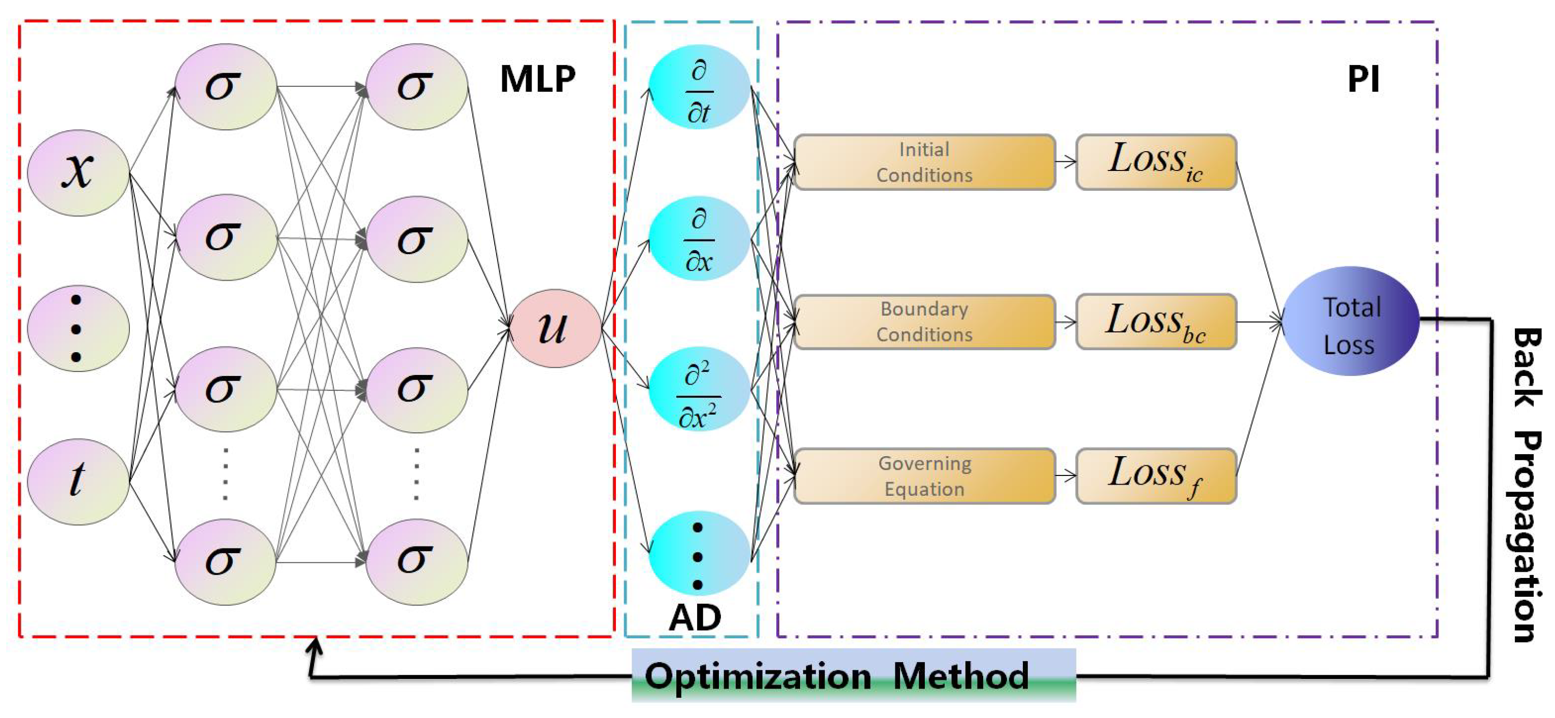
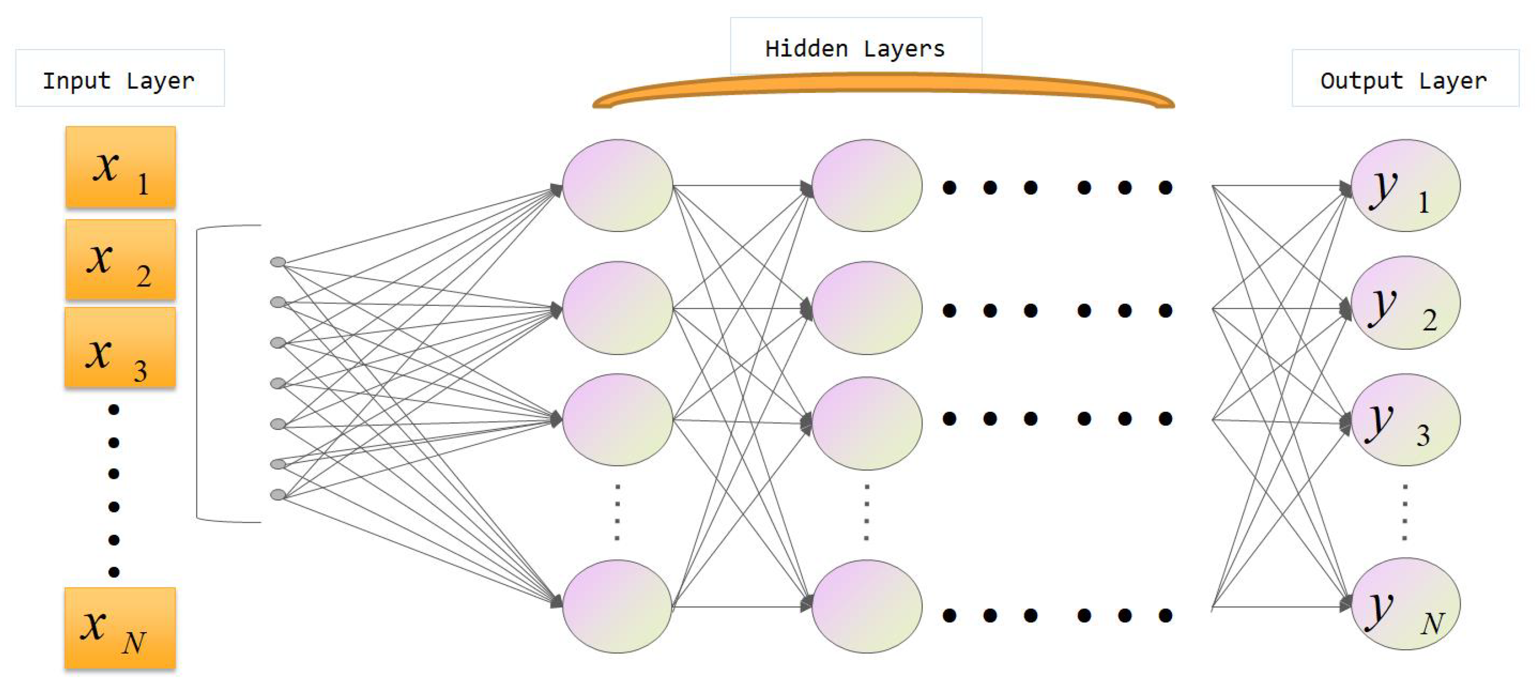
The classical PINNs framework is illustrated in Figure 1. The main network employs a multilayer feedforward fully connected neural network, as shown in Figure 2, to approximate the solution function $u(x,t)$. The core idea involves mapping the input $(x,t)$ through multiple layers of affine transformations and nonlinear activation functions to produce a prediction of the PDE solution. Partial derivatives are then computed via automatic differentiation to construct the PDE residual, thereby enhancing the interpretability of the fully connected network. In this study, a Multilayer Perception (MLP)-based network architecture is similarly adopted to construct the fPINNs framework.

3.3. fPINNs Algorithm Based on $L1$ Approximation

In Section 2, we have derived the $L1$ approximation scheme for the Caputo fractional derivative based on piecewise linear interpolation. Then, according to Equation (10), we obtain the iterative scheme

$$f(t_k)={\displaystyle \frac{\mathsf{\Gamma }(2-\alpha ){\tau }^{\alpha }}{a_0^{\left(\alpha \right)}}}\left[{ϵ}^2\mathsf{\Delta }u+\gamma (u-u^3)\right]+\sum _{l=1}^{k-1}{\displaystyle \frac{(a_{k-l-1}^{\left(\alpha \right)}-a_{k-l}^{\left(\alpha \right)})f\left(t_l\right)}{a_0^{\left(\alpha \right)}}}+{\displaystyle \frac{a_{k-1}^{\left(\alpha \right)}f\left(t_0\right)}{a_0^{\left(\alpha \right)}}},$$

(15)

which serves as the reference solution formulation for subsequent fPINNs simulations.

Next, the predicted solution of Equations (12)–(14) is obtained using the fPINNs solver. The output $\widehat{u}(x,t_k;\theta )$ of the fully connected network is directly taken as the approximate solution, leading to the following $L1$ approximation-based iterative formulation for the fPINNs:

$$F(t_k)={\displaystyle \frac{\mathsf{\Gamma }(2-\alpha ){\tau }^{\alpha }}{a_0^{\left(\alpha \right)}}}\left[{ϵ}^2\mathsf{\Delta }\widehat{u}+\gamma (\widehat{u}-{\widehat{u}}^3)\right]+\sum _{l=1}^{k-1}{\displaystyle \frac{(a_{k-l-1}^{\left(\alpha \right)}-a_{k-l}^{\left(\alpha \right)}){\widehat{u}}^l}{a_0^{\left(\alpha \right)}}}+{\displaystyle \frac{a_{k-1}^{\left(\alpha \right)}{\widehat{u}}^0}{a_0^{\left(\alpha \right)}}},$$

(16)

where $\widehat{u}=\widehat{u}(x,t_k;\theta )$; $\theta$ represents all learnable parameters in the fully connected network.

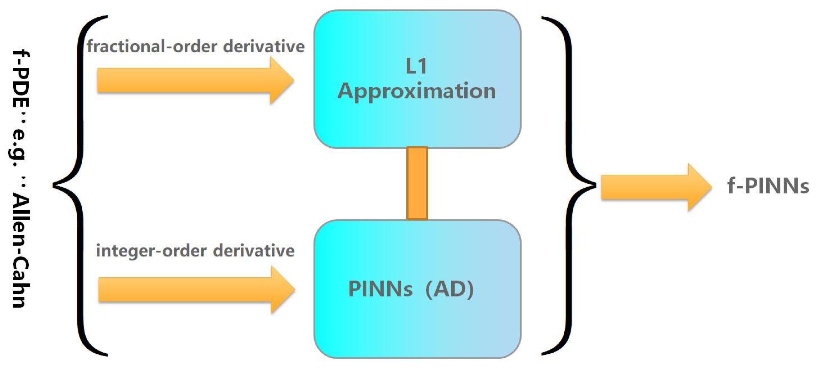
In summary, the specific solution framework of the $L1$ approximation-based fPINNs is illustrated in Figure 3. Integer-order derivatives of the neural network output are computed using automatic differentiation (as in PINNs), while fractional-order derivatives are numerically approximated via the $L1$ discretization scheme.

3.4. Loss Functions

In fPINNs, the parameters $\theta$ in $\widehat{u}(x,t;\theta )$ are trained by minimizing the following weighted sum of squared error,

$$\mathcal{L}\left(\theta \right)={\omega }_f{\mathcal{L}}_{PDE}+{\omega }_{ic}{\mathcal{L}}_{ic}+{\omega }_{bc}{\mathcal{L}}_{bc},$$

(17)

where, in practice, the weights ${\omega }_f$, ${\omega }_{ic}$, and ${\omega }_{bc}$ are typically initialized to 1 and then dynamically adjusted according to the magnitudes of the respective loss terms. The individual loss components are defined as follows:

• PDE residual loss ${\mathcal{L}}_{PDE}$. Define the residual function as

  $$r(x,t)={}_0{}^{C}D_t^{\alpha }\widehat{u}(x,t)-{ϵ}^2\mathsf{\Delta }\widehat{u}-\gamma (\widehat{u}-{\widehat{u}}^3).$$
  Then, the corresponding loss is given by

  $${\mathcal{L}}_{PDE}={\displaystyle \frac{1}{N_f}}\sum _{i=1}^{N_f}{r}^2(x_i,t_i),$$

  (18)

  where $N_f$ is the number of collocation points, and $(x_i,t_i)$ denotes the i-th specific sampling point. In fPINNs, this residual term is constructed by combining automatic differentiation with numerical discretization.
• Initial condition loss ${\mathcal{L}}_{ic}$,

  $${\mathcal{L}}_{ic}={\displaystyle \frac{1}{N_{ic}}}\sum _{i=1}^{N_{ic}}{(\widehat{u}(x_i,0)-u_0\left(x_i\right))}^2,$$

  (19)

  where $N_{ic}$ is the number of sampling points under the initial condition, and $x_i$ represents the i-th specific sampling point satisfying the initial condition.
• Boundary condition loss ${\mathcal{L}}_{bc}$,

  $${\mathcal{L}}_{bc}={\displaystyle \frac{1}{N_{bc}}}\sum _{i=1}^{N_{bc}}{(\widehat{u}(x_i^{bc},t_i^{bc})-u_b(x_i^{bc},t_i^{bc}))}^2,$$

  (20)

  where $N_{bc}$ is the number of sampling points under the boundary condition. $(x_i^{bc},t_i^{bc})$ denotes the i-th specific sampling point on the boundary. If $x_i^{bc}=0$, then $u_b=g_1$; if $x_i^{bc}=1$, then $u_b=g_2$.

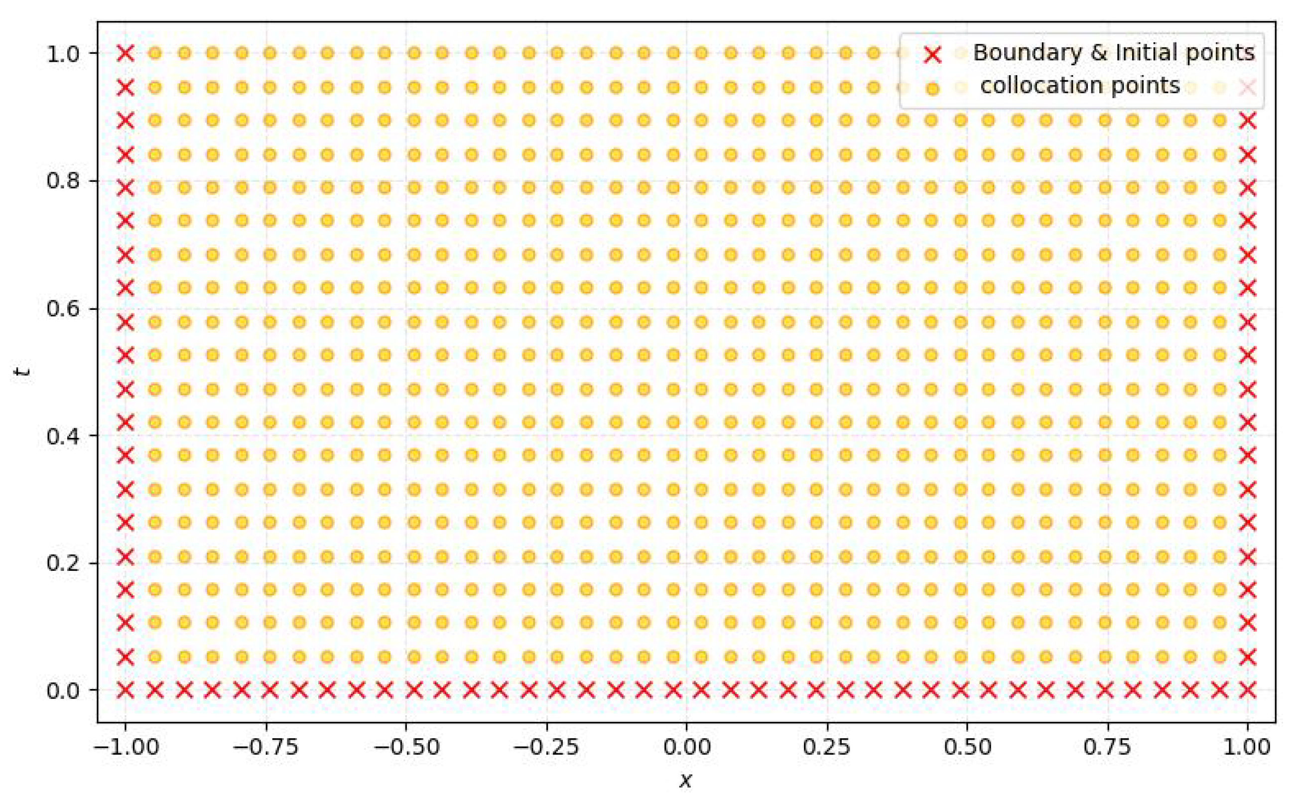
As an example for a one-dimensional spatial problem, the distribution of sample points is illustrated in Figure 4. The collection of these collocation points is fed into the neural network as a tensor input.

4. Improved Physics-Informed Neural Networks

In this section, to improve the computational accuracy and efficiency of fPINNs in solving the f–AC equation and f–CH equation, we propose three optimization strategies specifically tailored for the fPINNs framework. These strategies address neural network sampling, loss function weight assignment, and total loss optimization. The following subsections present an introduction to these optimization strategies and present the resulting improved fPINNs algorithm incorporating these improvements.

4.1. Optimization Strategies

4.1.1. Adaptive Non–Uniform Sampling(ANUS)

For the f–AC Equation (2) and f–CH Equation (3), uniform sampling may fail to effectively capture the rapid variations in the solution in specific regions (e.g., boundary layers or interfaces), leading to significant errors in these areas. In particular, the Caputo fractional derivative can cause errors to accumulate progressively throughout the network training process. Moreover, due to the nonlocal nature of fractional derivatives and the sharp gradient changes in interfacial regions (for example, near $x=0$), uniform grids tend to oversample smooth regions while suffering from insufficient resolution in critical areas.

To address this issue, we consider a non-uniform grid sampling method to enhance the capture of physical phenomena in specific regions (e.g., sharp transitions or boundary layers) of the f–AC equation. The core idea is to employ a higher density of sampling points in certain critical regions, such as the phase interface or initial temporal region, to resolve the solution with finer resolution in these areas. Specifically, the data sampling density is increased within a defined spatial region near the center to ensure accurate resolution of potential boundary layers or sharp variations. The remaining spatial domain is then divided into regions of moderate and low sampling density, where the solution is expected to vary more smoothly. This sampling strategy enables the generated dataset to improve the model’s ability to capture fine-scale physical features while maintaining computational efficiency.

4.1.2. Adaptive EMA Ratio Loss Weighting(AERLW)

In the loss function defined in Section 3.4, three components, that is, PDE residual loss ${\mathcal{L}}_{PDE}$, initial condition loss ${\mathcal{L}}_{ic}$, and boundary condition loss ${\mathcal{L}}_{bc}$, each have adjustable weighting coefficients. In typical solving scenarios, these weights are often set to fixed values. However, for more complex nonlinear equations, treating them as constants during network training may lead to imbalanced optimization, where certain loss terms dominate while others, particularly critical ones, fail to converge. For the Caputo derivative, the current residual incorporates influences from all previous time steps, causing the PDE residual error to accumulate progressively over the time domain. If the weights remain fixed or do not increase appropriately with time, the network may perform well at early time stages but deteriorate later as accumulated errors grow. Moreover, the nonlinear terms $\gamma (u-u^3)$ in the Equation (12) are often highly sensitive to errors within certain value ranges (for example, when the solution u is large or near saturation). Although the error contribution from these terms may initially be small, it can become a bottleneck during training. Fixed weights may thus fail to provide sufficient gradient drive when the network performs poorly on the nonlinear terms, resulting in inaccurate solutions near nonlinear saturation values.

To address this, inspired by the recent work [17,18], we propose a dynamic multi-objective loss weighting strategy. The main idea is to dynamically adjust the weights of individual loss components based on their relative magnitudes. During network training, this approach automatically balances the PDE residual loss with the boundary and initial condition losses, assigning higher weights to terms with larger losses so that they receive greater attention and are more adequately optimized. In contrast to conventional methods that update weights using instantaneous loss values, we employ an Exponential Moving Average (EMA) to smooth the loss value [19], which can reduce the impact of loss fluctuations and also can achieve more stable weight adaptation. The specific implementation steps are as follows:

• Compute the EMA of each loss component during the iterative process. The update formulas are

  $$\begin{array}{c}\hfill E_{ic}^{\left(t\right)}=\beta E_{ic}^{(t-1)}+(1-\beta ){\mathcal{L}}_{ic}^{\left(t\right)},\end{array}$$

  (21)

  $$\begin{array}{c}\hfill E_{bc}^{\left(t\right)}=\beta E_{bc}^{(t-1)}+(1-\beta ){\mathcal{L}}_{bc}^{\left(t\right)},\end{array}$$

  (22)

  $$\begin{array}{c}\hfill E_f^{\left(t\right)}=\beta E_f^{(t-1)}+(1-\beta ){\mathcal{L}}_{PDE}^{\left(t\right)},\end{array}$$

  (23)

  where $\beta$ is the decay rate of the EMA with a value in the range $(0,1)$. At initialization, we set $E_{ic}^{\left(0\right)}={\mathcal{L}}_{ic}^{\left(0\right)}$, $E_{bc}^{\left(0\right)}={\mathcal{L}}_{bc}^{\left(0\right)}$, and $E_f^{\left(0\right)}={\mathcal{L}}_{PDE}^{\left(0\right)}$.
• Compute the proportion of each EMA value as follows:

  $$\begin{array}{c}\hfill R_{ic}^{\left(t\right)}={\displaystyle \frac{E_{ic}^{\left(t\right)}}{E_{ic}^{\left(t\right)}+E_{bc}^{\left(t\right)}+E_f^{\left(t\right)}}},\end{array}$$

  (24)

  $$\begin{array}{c}\hfill R_{bc}^{\left(t\right)}={\displaystyle \frac{E_{bc}^{\left(t\right)}}{E_{ic}^{\left(t\right)}+E_{bc}^{\left(t\right)}+E_f^{\left(t\right)}}},\end{array}$$

  (25)

  $$\begin{array}{c}\hfill R_f^{\left(t\right)}={\displaystyle \frac{E_f^{\left(t\right)}}{E_{ic}^{\left(t\right)}+E_{bc}^{\left(t\right)}+E_f^{\left(t\right)}}},\end{array}$$

  (26)

  and update the weights according to

  $$\begin{array}{c}\hfill {\omega }_{ic}^{\left(t\right)}=(1-\eta ){\omega }_{ic}^{(t-1)}+\eta R_{ic}^{\left(t\right)},\end{array}$$

  (27)

  $$\begin{array}{c}\hfill {\omega }_{bc}^{\left(t\right)}=(1-\eta ){\omega }_{bc}^{(t-1)}+\eta R_{bc}^{\left(t\right)},\end{array}$$

  (28)

  $$\begin{array}{c}\hfill {\omega }_f^{\left(t\right)}=(1-\eta ){\omega }_f^{(t-1)}+\eta R_f^{\left(t\right)},\end{array}$$

  (29)

  where $\eta$ is the adaptation rate. The total loss function is then given by

  $$\begin{array}{c}\hfill {\mathcal{L}}^{\left(t\right)}={\omega }_f^{\left(t\right)}{\mathcal{L}}_{PDE}+{\omega }_{ic}^{\left(t\right)}{\mathcal{L}}_{ic}+{\omega }_{bc}^{\left(t\right)}{\mathcal{L}}_{bc}.\end{array}$$

  (30)
• Clipping coefficients. To prevent training instability caused by any single loss term becoming excessively large or small, we apply a clipping operation to ${\omega }_f$, ${\omega }_{ic}$ and ${\omega }_{bc}$. Let $\tilde{\omega }\in \{{\omega }_f,{\omega }_{ic},{\omega }_{bc}\}$; then,

  $$\begin{array}{c}\hfill \tilde{\omega }=\left\{\begin{array}{cc}0.01,\hfill & \mathrm{if}\tilde{\omega }<0.01,\hfill \\ \tilde{\omega },\hfill & \mathrm{if}0.01\le \tilde{\omega }\le 100,\hfill \\ 100,\hfill & \mathrm{if}\tilde{\omega }>100.\hfill \end{array}\right.\end{array}$$

  (31)

4.1.3. Two–Stage Adaptive Quasi Optimization (TAQO)

In traditional optimization, using only the Adam optimizer often leads to oscillations near the minimum or convergence to relatively “flat/less-accurate” regions. Conversely, using only the L–BFGS optimizer can make the solution highly sensitive to the initial point, potentially trapping the optimization in poor local minima or saddle points. To address these limitations, in this paper, we adopt a staged optimization strategy that combines the Adam and L-BFGS optimizers. The underlying idea is to first use the Adam optimizer to guide the parameters into a favorable basin of attraction and then employ the L–BFGS optimizer to achieve rapid convergence and high-accuracy refinement within this basin. In practice, we first perform pre-training with the Adam algorithm, followed by fine-tuning using the L–BFGS optimizer. This approach leverages the robustness of Adam and the curvature information (quasi-Newton properties) of L–BFGS in a complementary manner, yielding solutions that are more stable and accurate compared to using either optimizer alone.

4.2. Improved fPINNs Algorithm Based on Optimization Strategies

Based on the three optimization strategies proposed above, we first develop improved fPINNs algorithms incorporating each individual strategy. Since there are many strategy combinations, in this paper, we only choose two distinct combinations by comprehensively evaluating the accuracy improvement and computational efficiency (i.e., runtime reduction) achieved by each strategy thereby two new variants of the improved fPINNs algorithm are proposed.

4.2.1. Improved Fractional PINNs with Single Strategy

When only the first strategy is considered, we denote the f–ANUS–PINNs algorithm as the fPINNs framework with the ANUS. For the second strategy, the f–A–PINNs algorithm integrates the fPINNs framework with the AERLW method. At last, f–T–PINNs is denoted as the fPINNs framework with the TAQO strategy. Here, we only give the complete computational procedure for f–T–PINNs (Algorithm 1).

Algorithm 1 Algorithm: f–A–PINNs for Solving the f–AC Equation

Input: Spatiotemporal domain $\mathsf{\Omega }\times [0,T]$, fractional order $\alpha \in (0,1)$, model parameter $ϵ$ and $\gamma$, spatial and temporal discretization steps. Output: Predicted solution $\widehat{u}(x,t;\theta )$, relative $L^2$ error e. Algorithm steps: Generate training points. Discretize the computational domain and sample collocation points: PDE residual points: $(x_i^f,t_i^f)\in \mathsf{\Omega }\times (0,T],i=1,\dots ,N_f$; Initial condition points: $(x_i^{ic},0)\in \mathsf{\Omega },i=1,\dots ,N_{ic}$; Boundary condition points: $(x_i^{bc},t_i^{bc})\in \partial \mathsf{\Omega }\times [0,T],i=1,\dots ,N_{bc}$. Compute reference solution. Solve the f–AC equation using numerical scheme to obtain the reference solution $u(x,t)$ on the same grid. Initialize optimizer and parameters. Initialize neural network parameters $\theta$ (weights and biases), model parameters $\alpha$, $ϵ$, and $\gamma$. Set Training Stopping Criteria. Define the following termination conditions: Gradient tolerance: tolerance_grad; Maximum iterations: Epoch; Loss change threshold: tolerance_change. The training continues if any of the following is true: $\parallel {\nabla }_{\theta }{\mathcal{L}\left(\theta \right)\parallel }_2\ge \mathit{tolerance\_grad}$; Current iteration < Epoch; $|{\mathcal{L}}^{(k+1)}-{\mathcal{L}}^{\left(k\right)}|\ge {ϵ}_{\mathrm{machine}}$. Construct neural network and fPINNs framework. Build a deep feedforward fully connected neural network: $$\widehat{u}(x,t;\theta ):{\mathbb{R}}^2\to \mathbb{R}$$ with multiple hidden layers and nonlinear activation functions (e.g., tanh function); Approximate the Caputo fractional time derivative ${\partial }_t^{\alpha }u$ using the $L1$ scheme; Use PyTorch’s automatic differentiation to compute spatial and temporal derivatives required in the PDE residual. Define loss function with adaptive weights. The total loss is a weighted sum of residual components: $$\mathcal{L}(\theta ,\omega )={\omega }_f{\mathcal{L}}_{\mathrm{PDE}}+{\omega }_{ic}{\mathcal{L}}_{\mathrm{ic}}+{\omega }_{bc}{\mathcal{L}}_{\mathrm{bc}},$$ Initialize the loss weights: ${\omega }_f=100,{\omega }_{ic}=1,{\omega }_{bc}=1.$ Set the decay rate $\beta =0.01$ and weight update learning rate $\eta =0.5$. Optimize the loss function. Minimize $\mathcal{L}\left(\theta \right)$ using the L-BFGS optimizer to update the network parameters $\theta$ until convergence. Terminate training. Stop the optimization process when all stopping criteria are satisfied. Evaluate solution and Compute Error. Obtain the trained solution: $\widehat{u}(x,t;{\theta }^{*})$; Compute the relative $L^2$-norm error against the reference solution;

4.2.2. Fractional PINNs with AERLW and ANUS (f–A–A-PINNs) Algorithm

The f–A–A–PINNs algorithm enhances the accuracy and efficiency of solving the f-AC equation by integrating AERLW and ANUS strategies. The main procedure (Algorithm 2) is summarized below (only a brief description of the steps that are different from Algorithm 1 is provided).

Algorithm 2 Algorithm: f–A–A–PINNs: Solving the f–AC Equation

Algorithm steps: Generate Non–Uniform Training Grid (ANUS Strategy). Partition the spatial domain $\mathsf{\Omega }$ using a non-uniform grid to concentrate sampling in regions of expected high solution variation. For example,: if $\mathsf{\Omega }=[0,1]$, in $[0,0.05]$: assign N sampling points; In $[0.05,0.2]$: assign $N/2$ sampling points; In $[0.2,1]$: assign $N/4$ sampling points. Compute reference solution. Initialize optimizer and parameters. Set Training Termination Criteria: Construct neural network and fPINNs framework. Define loss function with adaptive weights (AERLW Strategy): Optimize the loss function. Terminate training. Evaluate solution and compute error.

4.2.3. Fractional PINNs with AERLW and TAQO (f–A–T–PINNs) Algorithm

The f–A–T–PINNs algorithm, which integrates the fPINNs method with the AERLW strategy and the TAQO strategy, is proposed to solve the f–AC equation. This algorithm is primarily based on Algorithm 1, with the addition of the TAQO strategy in step 7. Therefore, the detailed procedure of this algorithm is also omitted.

5. Numerical Experiments

In this section, we present the experimental results of solving the f–AC equation and the f–CH equation using the fPINNs framework and its improved versions based on $L1$ approximation. All experiments in this paper were conducted on an NVIDIA GeForce RTX 4090 GPU. The code was implemented in Python using the PyTorch framework. Unless otherwise specified, the structure of the neural network in the original fPINNs framework is listed as follows (

Table 1. The structure of original fPINNs.

Parameter	Value
Number of Hidden Layers	6
Number of Neurons per Layer	60
Activation function	tanh
Optimizer	L-BFGS
Learning rate	0.001

).

The relative $L^2$ error norm is adopted as the evaluation metric in the experiments,

$$e={\displaystyle \frac{\parallel \widehat{u}{-u\parallel }_{L^2}}{{\parallel u\parallel }_{L^2}}},$$

where $\widehat{u}$ is the predicted solution, u is the reference solution, and ${\parallel ·\parallel }_{L^2}$ is the $L^2$ norm.

5.1. fPINNs Algorithm for Solving f–AC Equation

Consider the following f–AC equation:

$${}_0{}^{C}D_t^{\alpha }u(x,t)={ϵ}^2\mathsf{\Delta }u+\gamma (u-u^3),$$

(32)

with the initial condition

$$u(x,0)=x^{2}cos\left(\pi x\right),$$

(33)

and the boundary conditions

$$u(0,t)=0,u(1,t)=-1.$$

(34)

Let the computational domain be $\mathsf{\Omega }=(x,t)\in [0,1]\times (0,1]$. Set $\alpha =0.5,ϵ=1$, $\gamma =5$, with a spatial step size of $1/60$ and a temporal step size of $1/60$. The fPINNs framework is employed to compute the predicted solution for Equations (32)–(34). Since Equations (32)–(34) do not have an exact analytical solution, the numerical solution based on the $L1$ scheme (11) is used as an approximate reference solution.

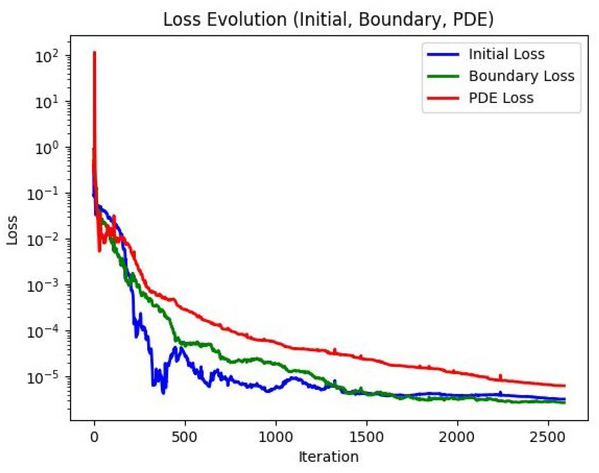
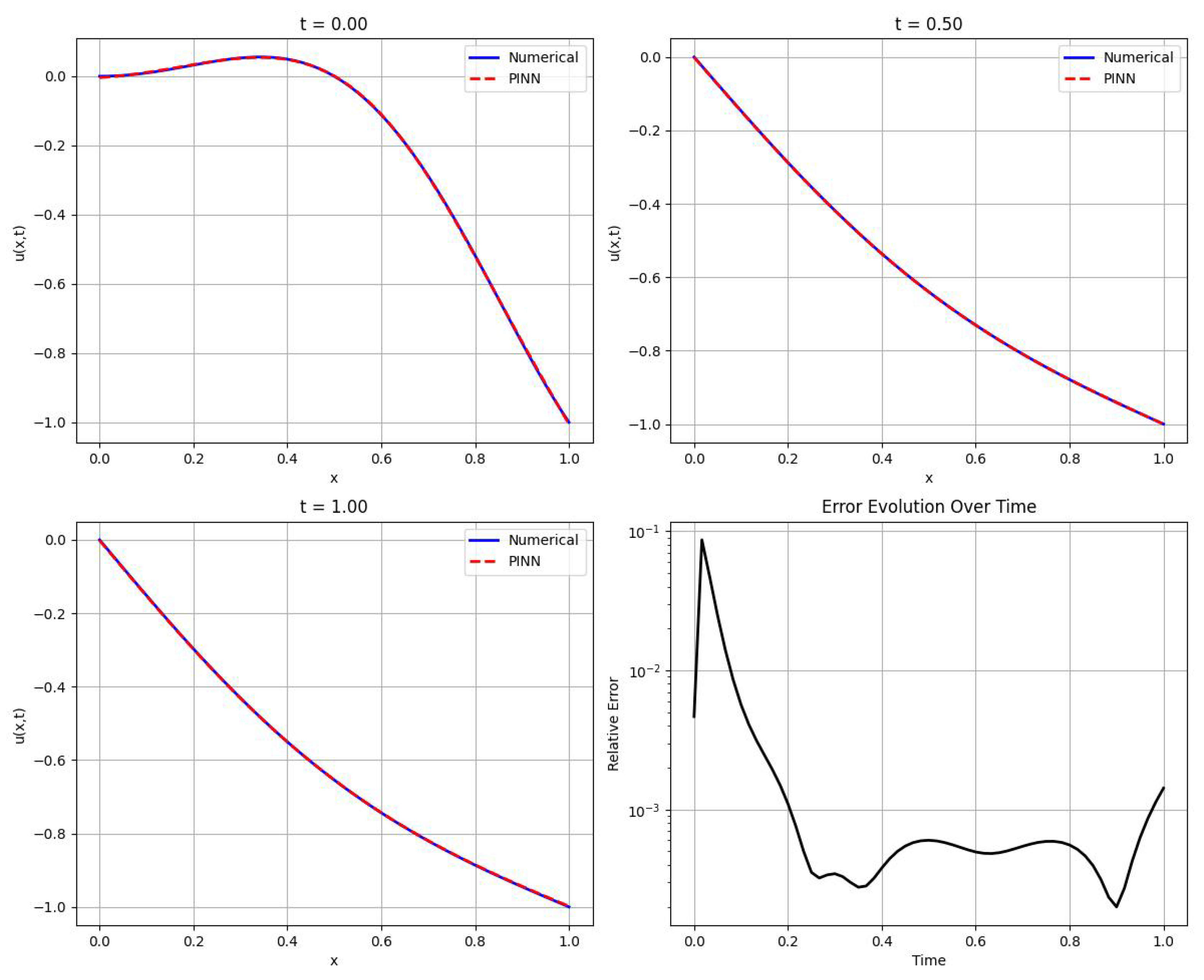
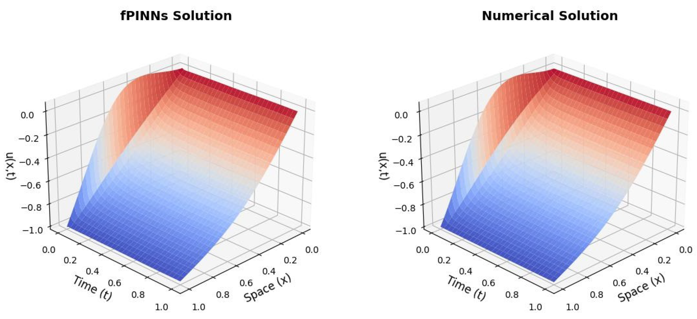
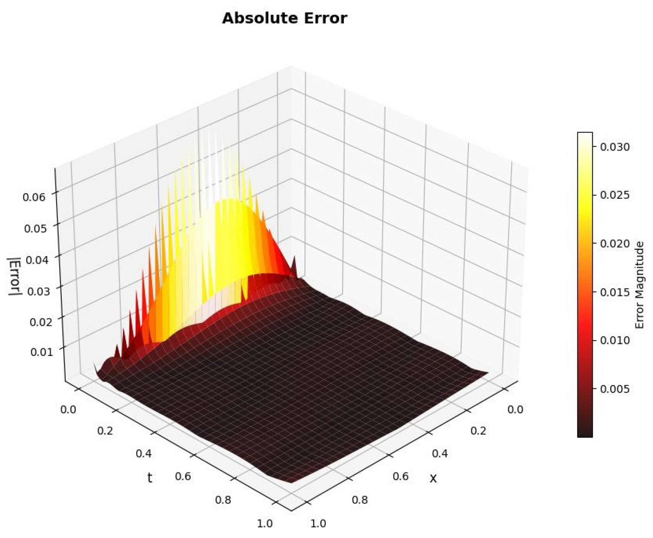
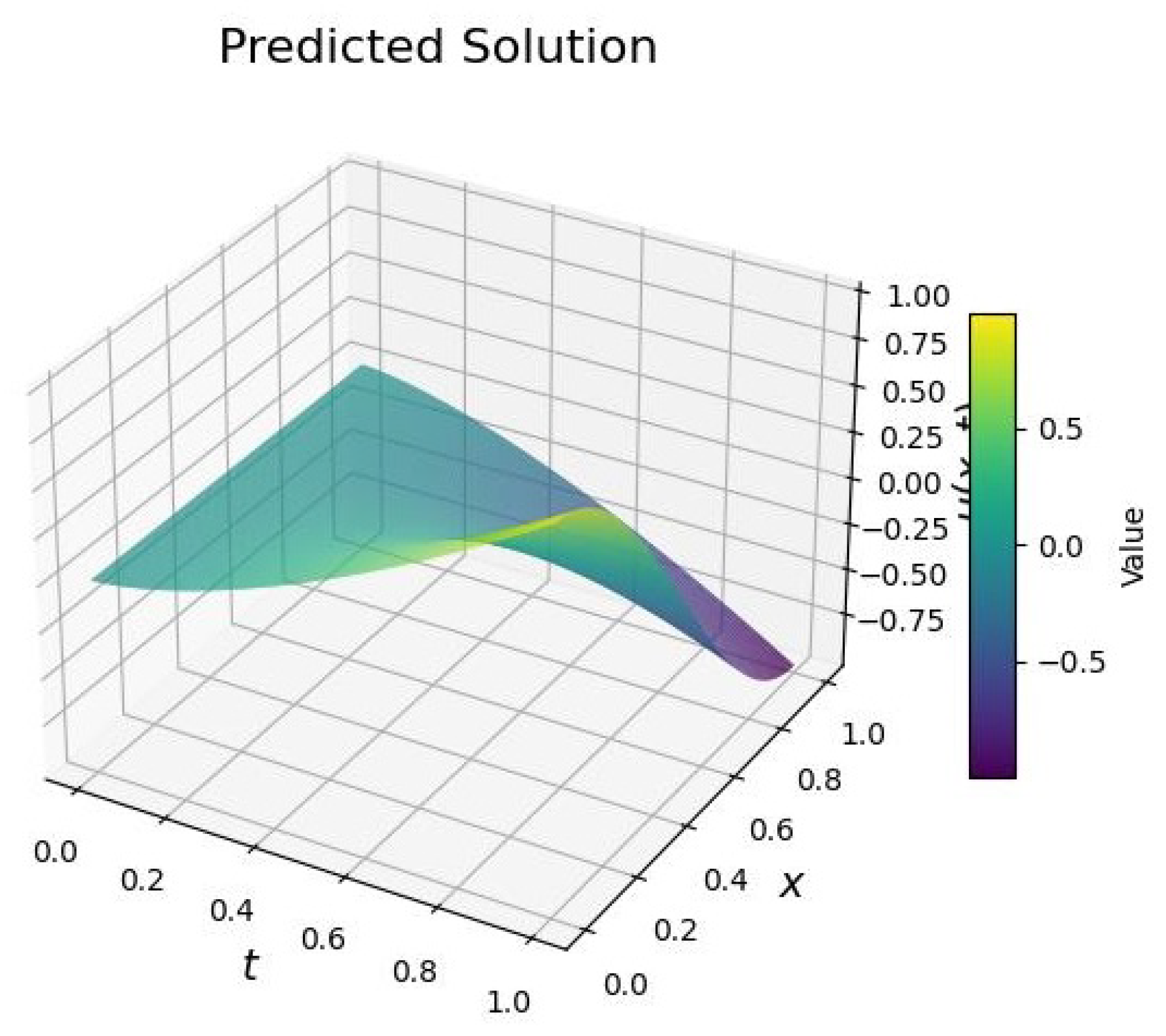
Throughout the computation, the relative error between the predicted solution and this reference is $1.053\times {10}^{-2}$. The evolution curves for the initial loss, boundary loss, and PDE loss are presented in Figure 5, along with the total loss curve shown in Figure 6. It can be observed from Figure 5 that all types of errors continuously decrease as the number of iterations increases. Figure 7 shows the predicted solution, the numerical solution, and their difference at three different times: $t=0$, $t=0.5$ and $t=1$. It is evident that the predicted solution agrees very well with the numerical solution at different times, demonstrating that the fPINNs algorithm can achieve high-accuracy results. In Figure 8, Figure 9 and Figure 10, a visualization of the predicted solution, the numerical solution, and their absolute error across the entire spatio-temporal domain are also provided.

To evaluate the stability of the fPINNs algorithm in solving the f–AC equation, its performance was assessed using different neural network parameters (specifically, the number of hidden layers and the number of neurons per layer). In

Table 2. The $L^2$ error of fPINNs employing neural networks of different sizes for the f-AC Equations (32)–(34) when $\alpha =0.5,ϵ=1,\gamma =5$.

Layers/Neurons	20	40	60	80
3	1.069 × 10−2	1.099 × 10−2	1.061 × 10−2	1.087 × 10−2
5	1.039 × 10−2	1.071 × 10−2	1.069 × 10−2	1.075 × 10−2
7	1.213 × 10−2	1.076 × 10−2	1.046 × 10−2	1.080 × 10−2
9	1.015 × 10−2	1.062 × 10−2	1.063 × 10−2	1.077 × 10−2

, the relative errors obtained with various network configurations are presented. The results indicate that the fPINNs algorithm exhibits minimal sensitivity to the choice of network parameters, as the prediction accuracy remains consistently high across different configurations.

5.2. Improved fPINNs Algorithm for Solving f–AC Equation

In Section 4.2, we proposed some improved fPINNs algorithms, namely, three improved fPINNs algorithms with a single strategy—f–ANUS-PINNs, f–A–PINNs and f–T–PINNs—and two combination algorithms—f–A–A–PINNs and f–A–T–PINNs. Using the same equation and parameters as in Section 5.1, the resulting $L^2$ errors obtained by each algorithm are summarized in

Table 3. $L^2$ error of fPINN and improved f-PINN algorithms for the f-AC Equations (32)–(34).

	Relative ${\mathit{L}}^2$ Error	Run Time (s)
fPINNs	1.053 × 10−2	428.22
f–ANUS-PINNs	1.033 × 10−2	405.79
f-A-PINNs	9.293 × 10−3	483.74
f-T-PINNs	1.088 × 10−2	318.34
f-A-A-PINNs	9.335 × 10−3	539.62
f-A-T-PINNs	8.476 × 10−3	853.21

.

According to the results presented in Table 3, among the three improved fPINNs algorithms employing a single strategy, both f–ANUS–PINNs and f–A–PINNs demonstrate the improvement in accuracy compared to the original fPINNs, with f–A–PINNs yielding superior computational performance relative to f–ANUS–PINNs.

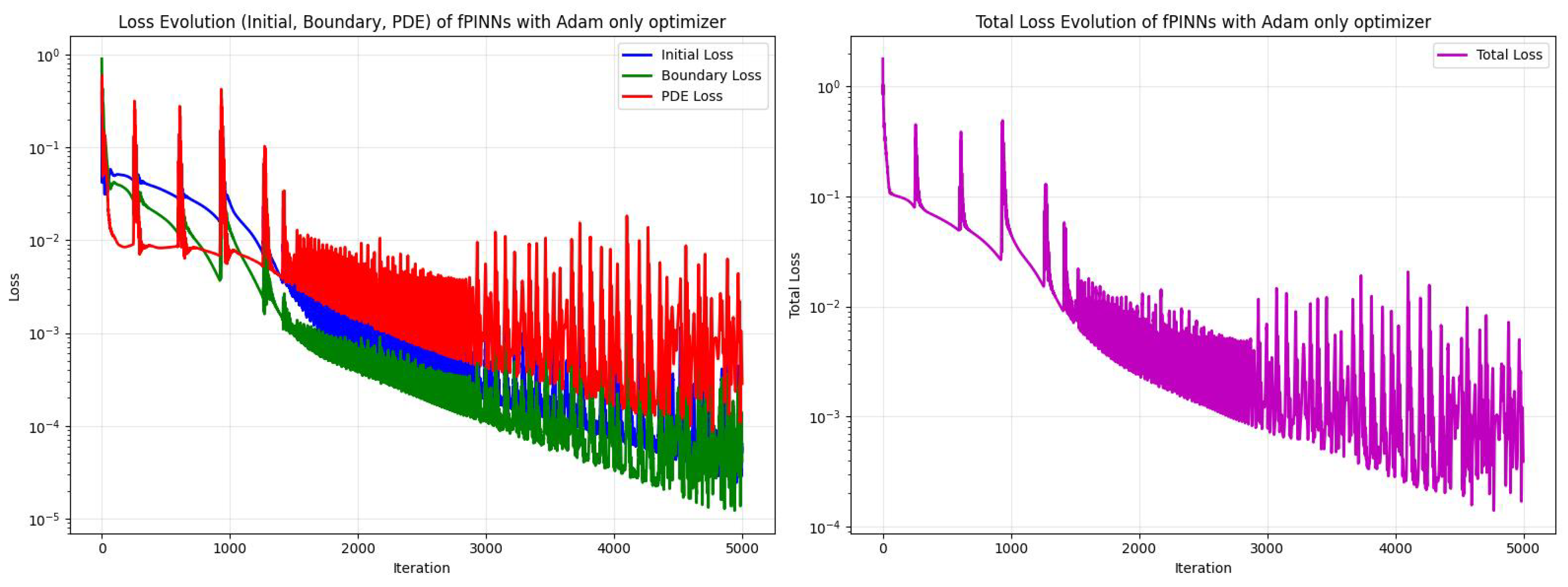
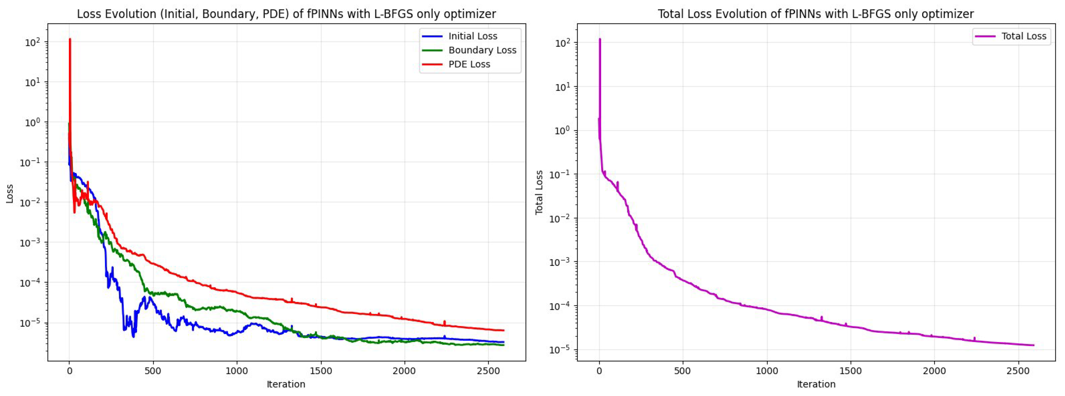
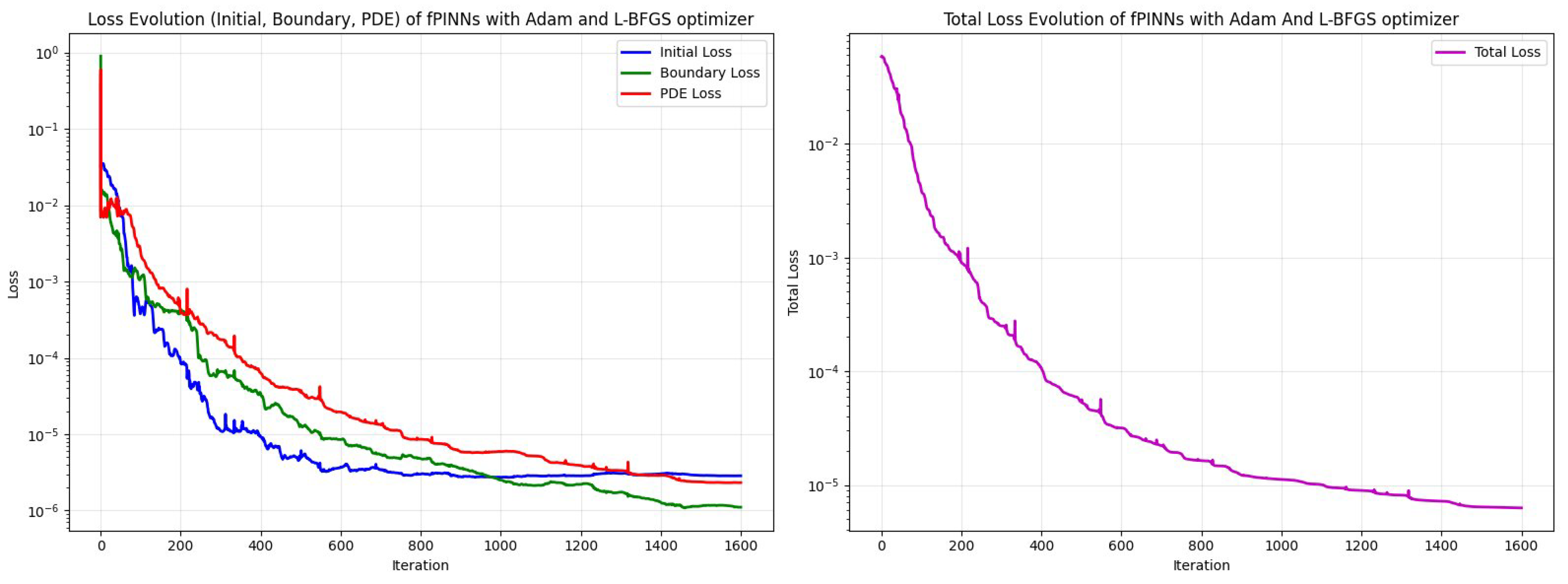
Also, we notice that the f–T–PINNs algorithm exhibits a slight degradation in accuracy, but it shows a notable advantage in terms of computational efficiency (i.e., reduced runtime). Here, we also present the loss curves of fPINNs with the Adam-only optimizer, fPINNs with L-BFGS-only (the default optimizer in this paper, see Table 1) and f-T-PINNs (with the Adam-L-BFGS optimizer) in Figure 11, Figure 12 and Figure 13.

As shown in Figure 11, Figure 12 and Figure 13, when only the Adam optimizer is used, each loss component begins to oscillate persistently after approximately 1200 iterations, and this oscillatory behavior continues even after 5000 iterations without convergence. In contrast, if we employ the L-BFGS-only optimizer, the oscillations observed with Adam can be avoided. However, it still requires a relatively large number of iterations to converge. By combining both optimizers, convergence is achieved in merely 1600 iterations, thereby significantly reducing computational time.

Consequently, for the algorithmic integration, we adopt the AERLW strategy as the primary component and combine it with the ANUS and TAQO strategies, respectively, resulting in two new variants: f–A–A–PINNs and f–A–T–PINNs. As evidenced by the results in Table 3, these combined variants consistently achieve higher accuracy than their single-strategy counterparts.

To further verify the stability of the improved fPINNs algorithms, next we only choose the original fPINNs and three improved algorithms, f–A–PINNs, f–A–A–PINNs and f–A–T–PINNs, to test the improved algorithms under different spatial and temporal step sizes.

5.2.1. Numerical Test for the Parameter $\alpha$

Fixed $ϵ=1$ and $\gamma =5$; to test the influence of the fractional order $\alpha$, we select different values of $\alpha$ and different time step sizes. The corresponding relative errors are shown in

Table 4. The $L^2$ error of fPINN and improved fPINN algorithms for $\alpha =0.35$.

${\mathit{N}}_{\mathit{t}}$	fPINNs	f-A-PINNs	f-A-A-PINNs	f-A-T-PINNs
21	2.718 × 10−2	2.773 × 10−2	2.702 × 10−2	2.684 × 10−2
31	2.189 × 10−2	2.194 × 10−2	2.122 × 10−2	2.148 × 10−2
41	1.809 × 10−2	1.749 × 10−2	1.864 × 10−2	1.763 × 10−2
61	1.419 × 10−2	1.519 × 10−2	1.616 × 10−2	1.382 × 10−2

,

Table 5. The $L^2$ error of fPINN and improved fPINN algorithms for $\alpha =0.6$.

${\mathit{N}}_{\mathit{t}}$	fPINNs	f–A–PINNs	f-A–A–PINNs	f–A–T–PINNs
21	2.185 × 10−2	2.106 × 10−2	1.916 × 10−2	2.145 × 10−2
31	1.616 × 10−2	1.403 × 10−2	1.472 × 10−2	1.481 × 10−2
41	1.273 × 10−2	1.085 × 10−2	1.118 × 10−2	1.225 × 10−2
61	8.705 × 10−3	7.128 × 10−3	7.609 × 10−3	8.039 × 10−3

and

Table 6. The $L^2$ error of fPINN and improved fPINN algorithms for $\alpha =0.8$.

${\mathit{N}}_{\mathit{t}}$	fPINNs	f–A–PINNs	f–A–A–PINNs	f–A–T–PINNs
21	1.7975 × 10−2	1.680 × 10−2	1.564 × 10−2	1.666 × 10−2
31	1.248 × 10−2	1.013 × 10−2	1.047 × 10−2	1.096 × 10−2
41	9.738 × 10−3	7.721 × 10−3	7.421 × 10−3	7.824 × 10−3
61	6.346 × 10−3	5.474 × 10−3	6.139 × 10−3	4.968 × 10−3

.

From Table 4, it can be observed that when the value of $\alpha$ is small, the performance of the f–A–PINNs algorithm is slightly inferior to that of the original fPINNs algorithm. This is primarily because a smaller $\alpha$ corresponds to a “slow diffusion” process, where the gradual state changes have little effect on the adjustment of loss weights. The redundant weight iterations lead to a decrease in computational accuracy. However, for larger values of $\alpha$, the weight adjustment becomes more significant for such “fast” diffusion processes.

In fact, for the f–AC equation, the initial condition loss ${\mathcal{L}}_{ic}$ at $t=0$ may be easily satisfied and thus have a small value. In contrast, the PDE residual loss ${\mathcal{L}}_{PDE}$ (which includes the fractional time derivative, the Laplacian term, and the nonlinear term) is evaluated over the entire spatial domain and may exhibit larger residuals. For a fixed weight ${\omega }_f$, if its value is too small, the ${\mathcal{L}}_{PDE}$ term may be neglected, causing the model to prioritize satisfying the initial and boundary conditions at the expense of PDE solution accuracy. Conversely, if ${\omega }_f$ is too large, the errors from the initial and boundary conditions may be overlooked during training. Therefore, dynamic weight adjustment can reasonably balance the three types of errors and achieve better computational performance.

Furthermore, as can be seen from the results in Table 4, Table 5 and Table 6, the f–A–A–PINNs algorithm generally outperforms the original fPINNs across most parameter combinations, except for cases with small values of $\alpha$ combined with small time step sizes. However, compared to the results in Table 6, for smaller $N_t$ values ($N_t=21,31,41$), the f–A–A–PINNs algorithm performs better than f-A-PINNs. In contrast, for larger $N_t$ values (e.g., $N_t=61$), the accuracy of the f–A–A–PINN algorithms slightly deteriorates.

In summary, the f–A–T–PINNs algorithm achieves higher accuracy than the original fPINNs algorithm across all combinations of $\alpha$ and $N_t$. Furthermore, the f–A–T–PINNs algorithm consistently outperforms both f-A-PINNs and f–A–A–PINNs and does not exhibit the accuracy fluctuations observed in the latter methods. The tests on the f–AC equation with the three hybrid optimization algorithms demonstrate that the f–A–T–PINNs approach yields the best overall performance, maintaining superior accuracy across multiple parameter configurations.

5.2.2. Numerical Test for the Parameter $\gamma$

In Equation (32), the parameter $\gamma$ represents the sharpness of the transition layer. In traditional numerical schemes, a larger value of $\gamma$ leads to increased computational difficulty. Therefore, we next test the stability of these algorithms with respect to the parameter $\gamma$. Fixing $ϵ=1$ and $\alpha =0.5$, the error results of the predicted solutions based on fPINNs and three improved fPINNs under different values of $\gamma$ are shown in

Table 7. The $L^2$ error of fPINN and improved fPINN algorithms for $\gamma =2$.

${\mathit{N}}_{\mathit{t}}$	fPINNs	f–A–PINNs	f–A–A–PINNs	f–A–T–PINNs
31	7.027 × 10−3	6.095 × 10−3	7.208 × 10−3	6.126 × 10−3
41	5.418 × 10−2	4.478 × 10−2	5.856 × 10−3	4.719 × 10−3
81	2.913 × 10−3	7.421 × 10−3	8.081 × 10−3	2.794 × 10−3
101	2.992 × 10−3	4.947 × 10−3	5.975 × 10−3	2.768 × 10−3

,

Table 8. The $L^2$ error of fPINN and improved fPINN algorithms for $\gamma =5$.

${\mathit{N}}_{\mathit{t}}$	fPINNs	f–A–PINNs	f–A–A–PINNs	f–A–T–PINNs
31	1.809 × 10−2	1.594 × 10−2	1.723 × 10−2	1.759 × 10−2
41	1.460 × 10−2	1.402 × 10−2	1.375 × 10−2	1.338 × 10−2
81	8.482 × 10−3	7.057 × 10−3	7.341 × 10−3	7.116 × 10−3
101	7.203 × 10−3	1.026 × 10−2	9.183 × 10−3	6.861 × 10−3

and

Table 9. The $L^2$ error of fPINN and improved fPINN algorithms for $\gamma =8$.

${\mathit{N}}_{\mathit{t}}$	fPINNs	f–A–PINNs	f–A–A–PINNs	f–A–T–PINNs
31	2.883 × 10−2	2.835 × 10−2	2.831 × 10−2	2.714 × 10−2
41	2.395 × 10−2	2.297 × 10−2	2.262 × 10−2	2.325 × 10−2
81	1.416 × 10−2	1.343 × 10−2	1.362 × 10−2	1.372 × 10−2
101	1.176 × 10−2	1.248 × 10−2	1.131 × 10−2	9.519 × 10−3

.

As can be observed from the results presented in Table 7, Table 8 and Table 9, fPINNs and the other three improved algorithms demonstrate satisfactory computational accuracy across different values of $\gamma$. However, according to Table 7, for larger values of $N_t$, the errors obtained by the f–A–PINNs and f–A–A–PINNs algorithms increase. This may be attributed to the smaller time-step size, which results in a slower diffusion process in state evolution, thereby degrading the accuracy of these two enhanced algorithms. In contrast, for larger values of $\gamma$, as shown in Table 8 and Table 9, all three improved algorithms generally outperform the original fPINNs. Among the three improved algorithms, f-A–T–PINNs exhibits the greatest stability with respect to the parameter $\gamma$.

5.3. f–A–T–PINNs Algorithm for Solving 2D f–AC Equation

Based on the performance comparison presented in Section 5.2, we select the f–A–T–PINNs algorithm in this section for solving the 2D f–AC equation. Consider the following 2D f–AC equation:

$${}_0{}^{C}D_t^{\alpha }u(x,y,t)={ϵ}^2\mathsf{\Delta }u+\gamma (u-u^3)+f(x,y,t),(x,y)\in \mathsf{\Omega },t\in [0,T]$$

(35)

where $\mathsf{\Omega }=[0,1]\times [0,1],T=1$. When $ϵ=0.1$ and $\gamma =1$, the exact solution of Equation (35) is

$$u(x,y,t)=0.2(t^2+1)cos\left(\pi x\right)cos\left(\pi y\right),$$

(36)

and the initial function and the boundary function can be obtained directly. The source function $f(x,y,t)$ is

$$\begin{array}{c}\hfill f(x,y,t)={\displaystyle \frac{0.4cos\left(\pi x\right)cos\left(\pi y\right)}{\mathsf{\Gamma }(3-\alpha )}}{t}^{2-\alpha }+0.004\pi (t^2+1)cos\left(\pi x\right)cos\left(\pi y\right)\\ \hfill +0.01[({(0.2(t^2+1)cos(\pi x)cos(\pi y))}^2-1)·0.2·(t^2+1)cos(\pi x)cos(\pi y)].\end{array}$$

(37)

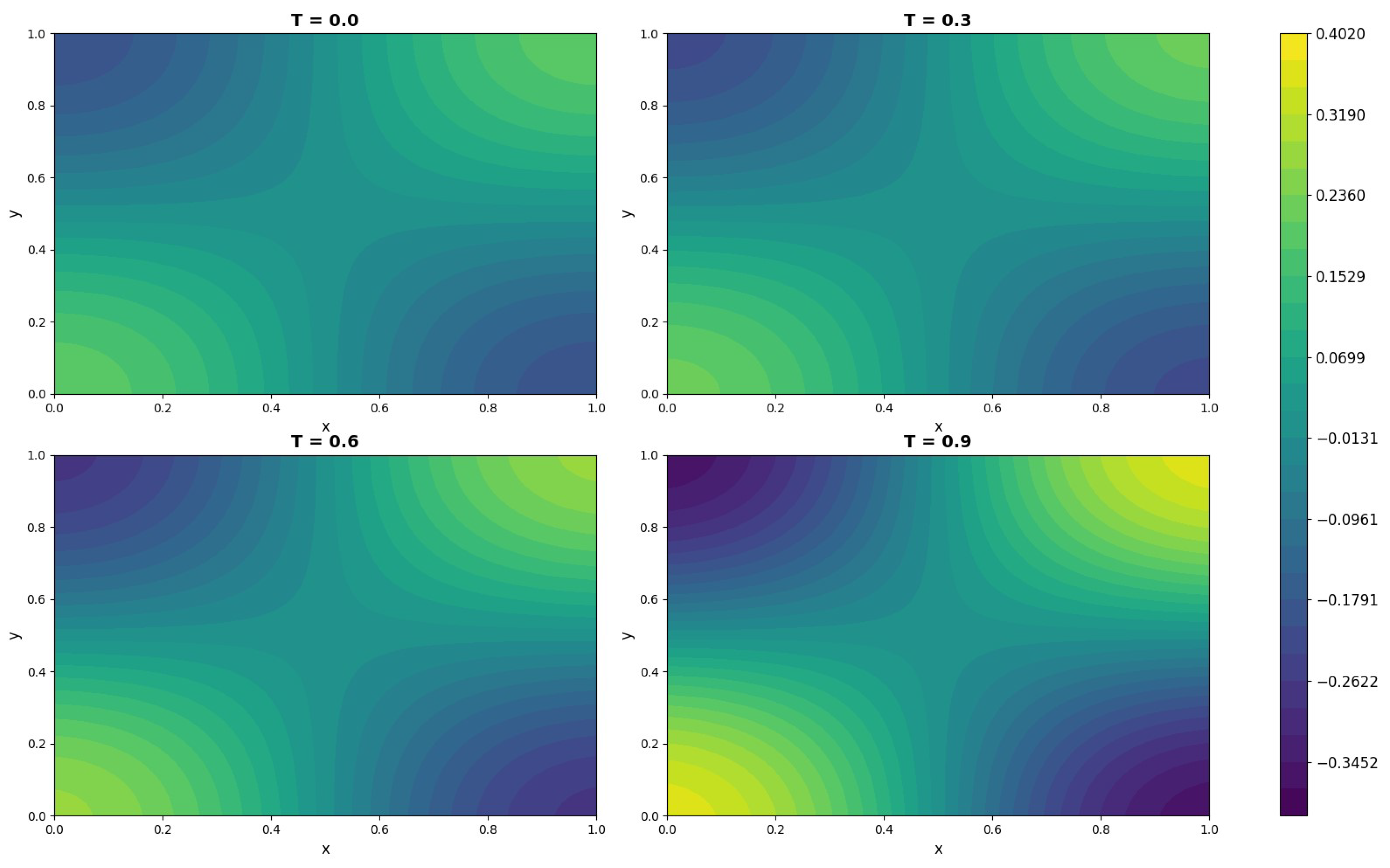
Choose $\alpha =0.9,ϵ=1$ and $\gamma =5$. The temporal and spatial step sizes are both $1/32$. The 2D f-AC equation is solved using both the fPINN and f–A–T–PINN algorithms, respectively, and the resulting relative errors and the run time are presented in the following

Table 10. The $L^2$ error and run time of fPINN and f-A-T-PINN algorithms for the 2D f–AC Equation (35).

	fPINNs	f-A-T-PINNs
Relative $L^2$ error	3.399 × 10−2	1.921 × 10−2
RUn time(s)	376.84	538.18

. In Figure 14 and Figure 15, a visualization of the exact solution, the numerical solution, and the evolution of the numerical solution with f–A–T-PINNs for Equation (35) are provided.

According to the results in Table 2 and Table 10, the computational time required by the fPINNs algorithm to solve the 2D f-AC equation is comparable to that for the 1D case, while achieving satisfactory numerical accuracy. This demonstrates the advantage of fPINNs in handling high-dimensional problems. Moreover, although the improved f-A-T-PINNs algorithm incurs additional computational cost, it further reduces the numerical error.

5.4. f–A–T–PINNs Algorithm for Solving the f–CH Equation

In this section, we also select the f–A–T–PINN algorithm for solving the f–CH equation. Consider the following f–CH equation:

$$\begin{array}{c}\hfill {}_0{}^{C}D_t^{\alpha }u(x,t)=-{ϵ}^2{\displaystyle \frac{{\partial }^{4}u}{\partial x^4}}+\gamma {\displaystyle \frac{{\partial }^2\varphi \left(u\right)}{\partial x^2}}+f(x,t),(x,t)\in \mathsf{\Omega }=[0,1]\times (0,1]\end{array}$$

(38)

with the initial condition

$$u(x,0)=0,x\in [0,1],$$

(39)

and the boundary conditions

$$u(0,t)=t^{1+\alpha },u(1,t)=-t^{1+\alpha },{\displaystyle \frac{\partial u}{\partial x}}(0,t)={\displaystyle \frac{{\partial }^{3}u}{\partial x^3}}(0,t)=0,t\in [0,1],$$

(40)

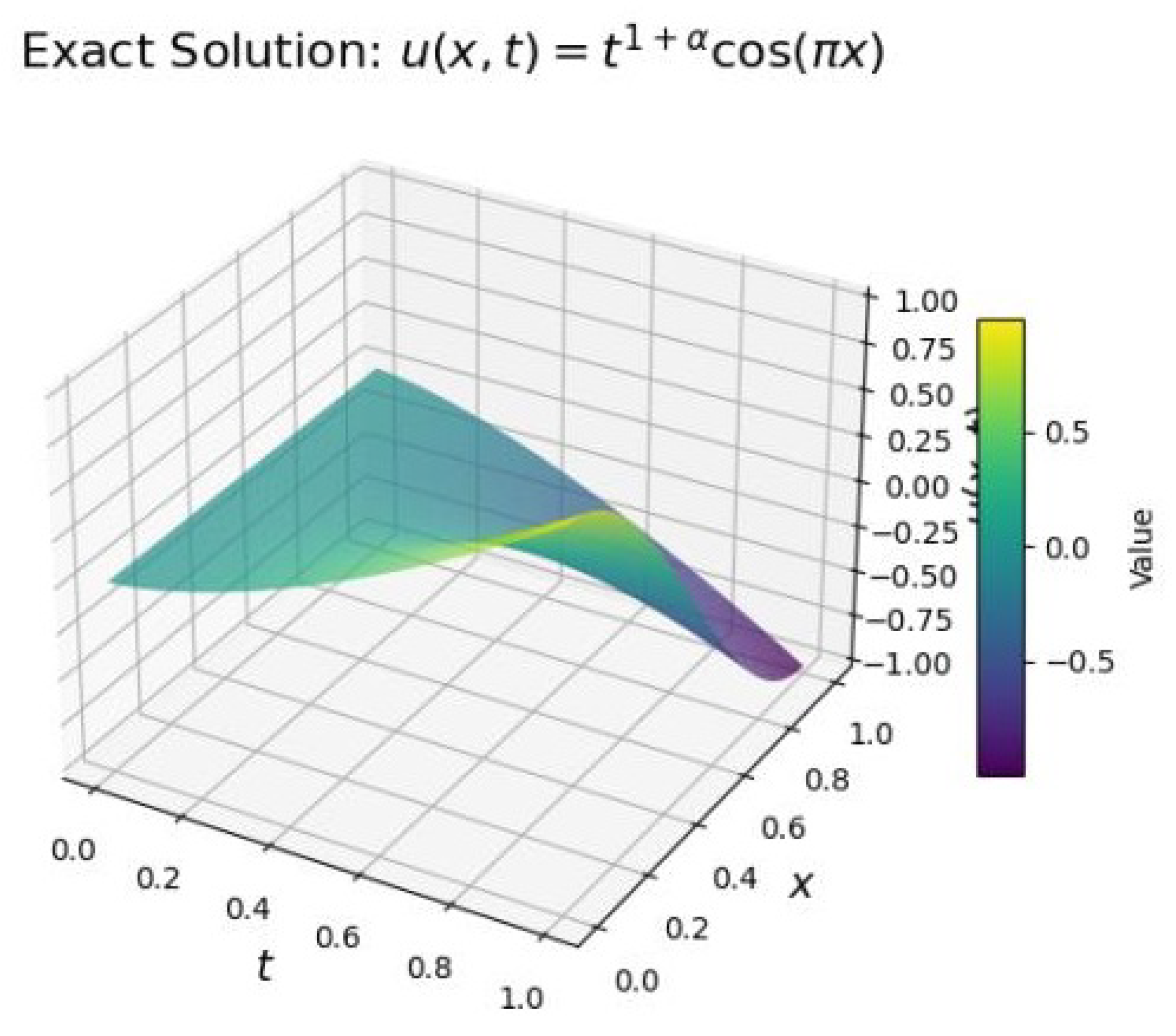
where $\varphi \left(u\right)=u^3-u$; the exact solution is $u(x,t)=t^{1+\alpha }cos\left(\pi x\right)$, and the source term $f(x,t)$ is given by

$$\begin{array}{c}\hfill f(x,t)=\mathsf{\Gamma }(2+\alpha )tcos\left(\pi x\right)+({ϵ}^2{\pi }^2-\gamma ){\pi }^2{t}^{1+\alpha }cos\left(\pi x\right)\\ \hfill -3\gamma {\pi }^{2}cos\left(\pi x\right)[2{sin}^2\left(\pi x\right)-{cos}^2\left(\pi x\right)]t^{3+3\alpha }.\end{array}$$

(41)

Due to the inclusion of derivative boundary conditions, the loss function within the f–A–T–PINN framework is modified as

$$\begin{array}{c}\hfill \mathcal{L}={\omega }_f{\mathcal{L}}_{PDE}+{\omega }_{ic}{\mathcal{L}}_{ic}+{\omega }_{bc}{\mathcal{L}}_{bc}+{\omega }_{fdbc}{\mathcal{L}}_{fdbc}+{\omega }_{tdbc}{\mathcal{L}}_{tdbc},\end{array}$$

(42)

where ${\mathcal{L}}_{fdbc}$ is the loss term for the first-order derivative boundary condition with corresponding weight ${\omega }_{fdbc}$, and ${\mathcal{L}}_{tdbc}$ is the loss term for the third-order derivative boundary condition with corresponding weight ${\omega }_{tdbc}$. In the improved algorithm under the f–A–T–PINN framework, the initial weights are set as

$${\omega }_f=1,{\omega }_{ic}=10,{\omega }_{bc}=10,{\omega }_{fdbc}=0.1,{\omega }_{tdbc}=0.01.$$

(43)

${\mathcal{L}}_{ic}$ and ${\mathcal{L}}_{bc}$ are defined as in Equations (19) and (20), respectively. Other loss components are defined as follows:

PDE residual loss ${\mathcal{L}}_{PDE}$: Define the residual function

$$r(x,t)={}_0{}^{C}D_t^{\alpha }\widehat{u}(x,t)+{\epsilon }^2{\displaystyle \frac{{\partial }^4\widehat{u}(x,t)}{\partial x^4}}-{\displaystyle \frac{{\partial }^2\varphi \left(\widehat{u}(x,t)\right)}{\partial x^2}}-f(x,t),$$

(44)

and the corresponding loss is

$${\mathcal{L}}_{PDE}={\displaystyle \frac{1}{N_f}}\sum _{i=1}^{N_f}{(r(x_i^{(f)},t_i^{(f)}))}^2.$$

(45)

First-order derivative boundary condition loss ${\mathcal{L}}_{fdbc}$:

$${\mathcal{L}}_{fdbc}={\displaystyle \frac{1}{N_{fdbc}}}\sum _{i=1}^{N_{fdbc}}{\left({\displaystyle \frac{\partial \widehat{u}(x_i^{(fdbc)},t_i^{(fdbc)})}{\partial x}}-{\displaystyle \frac{\partial u(x_i^{(fdbc)},t_i^{(fdbc)})}{\partial x}}\right)}^2,$$

(46)

where $N_{fdbc}$ is the number of sampling points, $\partial \widehat{u}/\partial x$ is the network’s predicted output, and $\partial u/\partial x$ is the predefined first-order derivative boundary condition.

Third-order derivative boundary condition loss ${\mathcal{L}}_{tdbc}$:

$${\mathcal{L}}_{tdbc}={\displaystyle \frac{1}{N_{tdbc}}}\sum _{i=1}^{N_{tdbc}}{\left({\displaystyle \frac{{\partial }^3\widehat{u}(x_i^{(tdbc)},t_i^{(tdbc)})}{\partial x^3}}-{\displaystyle \frac{{\partial }^{3}u(x_i^{(tdbc)},t_i^{(tdbc)})}{\partial x^3}}\right)}^2,$$

(47)

where $N_{tdbc}$ is the number of sampling points, ${\partial }^3\widehat{u}/\partial x^3$ is the network’s predicted output, and ${\partial }^{3}u/\partial x^3$ is the predefined third-order derivative boundary condition.

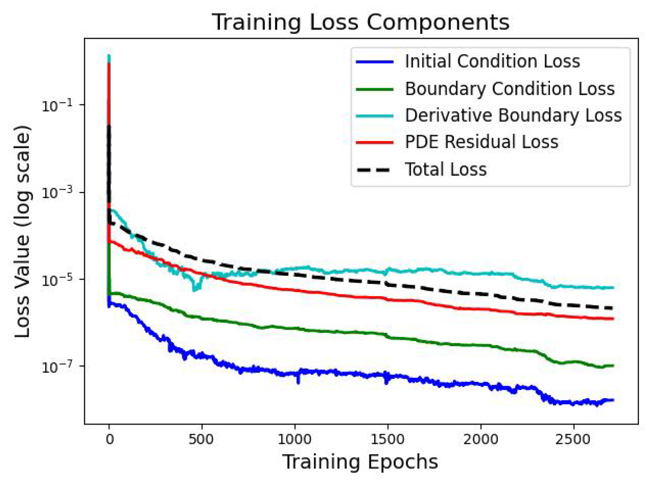
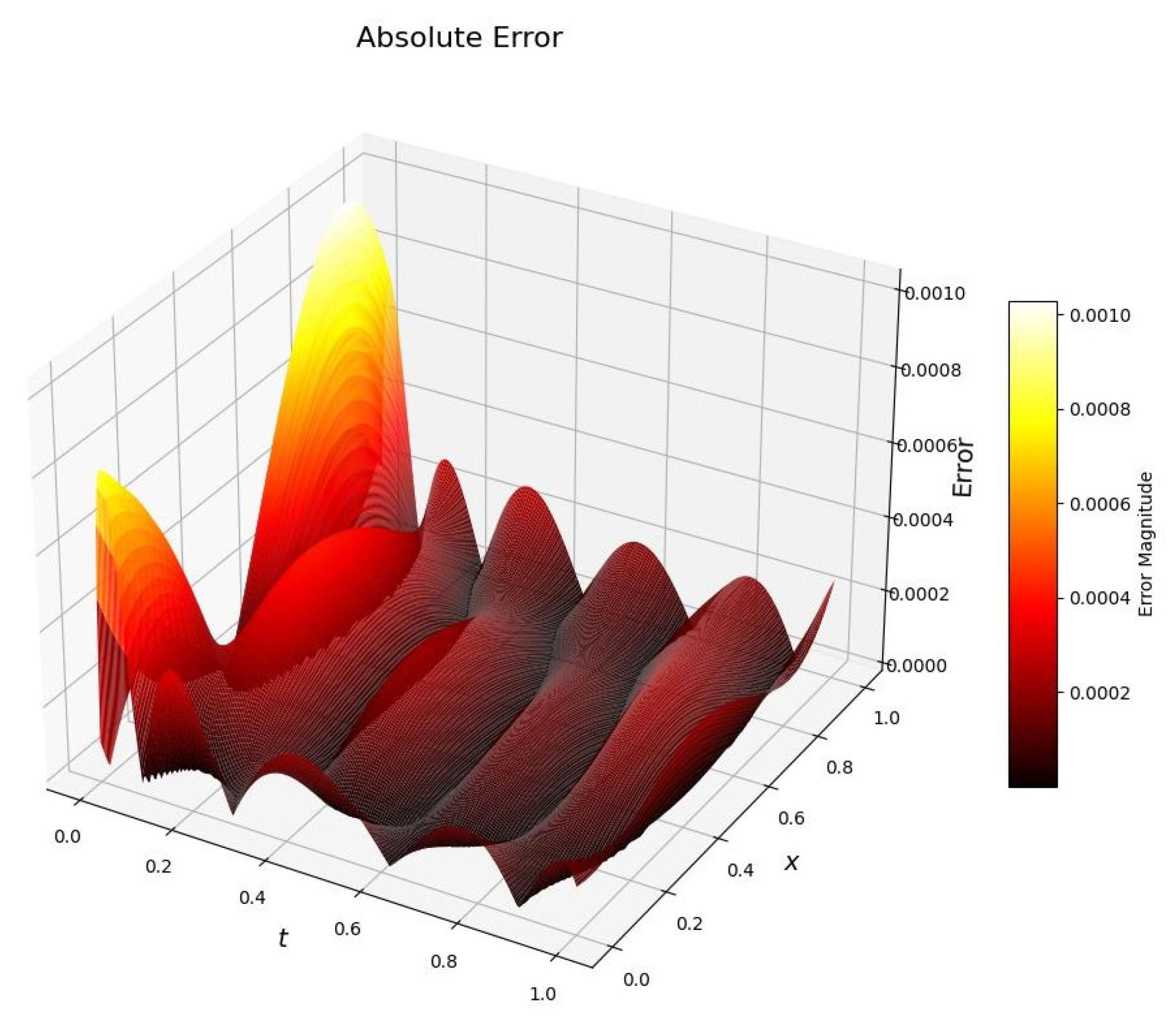
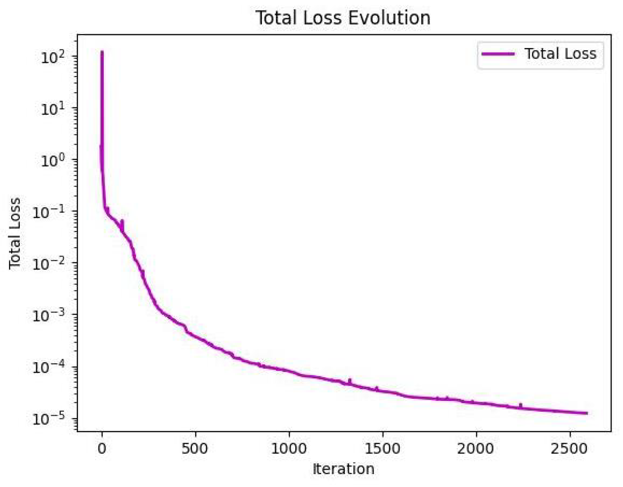
Set $\alpha =0.5$, $\epsilon =0.1$, with a spatial step size of $1/100$ and a temporal step size of $1/100$. The f-CH equation is solved using both the fPINN and f–A–T–PINN algorithms, respectively. and the resulting relative errors are presented in the following

Table 11. The $L^2$ error of fPINN and f-A-T-PINN algorithms for the f-CH Equations (38)–(40).

	fPINNs	f-A-T-PINNs
Relative $L^2$ error	8.323 × 10−3	5.219 × 10−4

. The exact solution of Equations (38)–(40) and the corresponding predicted solution with f–A–T–PINNs are presented in Figure 16 and Figure 17, respectively. Each loss and total loss are also plotted in Figure 18 and Figure 19, and the absolute error between the exact solution and the predicted solution is shown in Figure 20, respectively.

As can be seen from Table 11, for the higher-order f–CH equation, the f–A–T–PINNs algorithm achieves higher accuracy than the fPINNs algorithm, and the performance improvement is more effective compared to that observed in solving the f–AC equation.

6. Conclusions

Due to the nonlinearity and stiffness of the f–AC and f–CH equations, as well as the nonlocal nature of the $L1$ discretization scheme for the Caputo fractional derivative, this study employs the fPINNs algorithm to conduct numerical investigations on these two prototypical fractional gradient flow models. To enhance the solution accuracy of fPINNs, three optimization strategies are proposed to improve the network architecture, leading to the development of three improved fPINNs algorithms based on combinations of these strategies. Numerical examples demonstrate that the proposed algorithms achieve varying degrees of improvement over the original fPINNs, with the f–A–T–PINNs algorithm exhibiting superior numerical accuracy and enhanced stability with respect to parameter variations.

This work focuses exclusively on optimizing the fPINNs algorithm based on the $L1$ approximation. Based on existing research, future efforts will extend to the development of fPINNs algorithms incorporating fast numerical schemes that overcome the initial singularity and reduce high computational cost, such as the fast L1 (or $L2-1_{\sigma }$) formula with SOE technique [20,21], the parallel-in-time method [22], the spectral collocation method [14] and the finite element method [23], to further improve accuracy and efficiency.

References

1. Raissi, M.; Perdikaris, P.; Karniadakis, G.E. Physics–informed Neural Networks: A deep learning framework for solving forward and inverse problems involving nonlinear partial differential equations. J. Comput. Phys. 2019, 378, 686–707. [Google Scholar] [CrossRef]
2. Lu, L.; Pestourie, R.; Yao, W.J.; Wang, Z.C.; Verdugo, F.; Johnson, S.G. Physics–informed neural networks with hard constraints for inverse design. SIAM J. Sci. Comput. 2021, 43, B1105–B1132. [Google Scholar] [CrossRef]
3. Pang, G.F.; Lu, L.; Karniadakis, G.E. fPINNs: Fractional physics–informed neural networks. SIAM J. Sci. Comput. 2019, 41, A2603–A2626. [Google Scholar] [CrossRef]
4. Zhang, J.N.; Zhao, Y.; Tang, Y.F. Adaptive loss weighting auxiliary output fPINNs for solving fractional partial integro–differential equations. Phys. D–Nonlinear Phenom. 2024, 460, 134066. [Google Scholar] [CrossRef]
5. Yan, X.B.; Xu, Z.Q.J.; Ma, Z. Laplace–fPINNs: Laplace-based fractional physics–informed neural networks for solving forward and inverse problems of a time fractional equation. East Asian J. Appl. Math. 2024, 14, 657–674. [Google Scholar] [CrossRef]
6. Guo, L.; Wu, H.; Yu, X.C.; Zhou, T. Monte Carlo fPINNs: Deep learning method for forward and inverse problems involving high dimensional fractional partial differential equations. Comput. Methods Appl. Mech. Eng. 2022, 400, 115523. [Google Scholar] [CrossRef]
7. Du, Q.; Yang, J.; Zhou, Z. Time–fractional Allen–Cahn equations: Analysis and numerical methods. J. Sci. Comput. 2020, 85, 42. [Google Scholar] [CrossRef]
8. Liao, H.L.; Tang, T.; Zhou, T. An energy stable and maximum bound preserving scheme with variable time steps for time fractional Allen–Cahn equation. SIAM J. Sci. Comput. 2021, 43, A3130–A3155. [Google Scholar] [CrossRef]
9. Zhang, G.Y.; Huang, C.M.; Alikhanov, A.A.; Yin, B.L. A high–order discrete energy decay and maximum-principle preserving scheme for time fractional Allen–Cahn equation. J. Sci. Comput. 2023, 96, 39. [Google Scholar] [CrossRef]
10. Liu, H.; Cheng, A.J.; Wang, H.; Zhao, J. Time–fractional Allen–Cahn and Cahn–Hilliard phase–field models and their numerical investigation. Comput. Math. Appl. 2018, 76, 1876–1892. [Google Scholar] [CrossRef]
11. Zhang, J.; Zhao, J.; Wang, J.R. A non-uniform time–stepping convex splitting scheme for the time–fractional Cahn–Hilliard equation. Comput. Math. Appl. 2020, 80, 837–850. [Google Scholar] [CrossRef]
12. Ran, M.H.; Zhou, X.Y. An implicit difference scheme for the time–fractional Cahn–Hilliard equations. Math. Comput. Simulat. 2021, 180, 61–71. [Google Scholar] [CrossRef]
13. Wight, C.L.; Zhao, J. Solving Allen–Cahn and Cahn–Hilliard equations using the adaptive physics informed neural networks. Commun. Comput. Phys. 2021, 29, 930–954. [Google Scholar] [CrossRef]
14. Wang, S.P.; Zhang, H.; Jiang, X.Y. Fractional physics–informed neural networks for time–fractional phase field models. Nonlinear Dyn. 2022, 110, 2715–2739. [Google Scholar] [CrossRef]
15. Wang, X.; Wang, X.P.; Qi, H.T.; Xu, H.Y. Numerical simulation of time fractional Allen–Cahn equation based on Hermite neural solver. Appl. Math. Comput. 2025, 491, 129234. [Google Scholar] [CrossRef]
16. Podlubny, I. Fractional Differential Equations: An Introduction to Fractional Derivatives, Fractional Differential Equations, to Methods of Their Solution and Some of Their Applications; Elsevier: Amsterdam, The Netherlands, 1998. [Google Scholar]
17. McClenny, L.D.; Braga-Neto, U.M. Self–adaptive physics–informed neural networks. J. Comput. Phys. 2023, 474, 111722. [Google Scholar] [CrossRef]
18. Berardi, M.; Difonzo, F.; Icardi, M. Inverse physics–informed neural networks for transport models in porous materials. Comput. Methods Appl. Mech. Eng. 2025, 435, 117628. [Google Scholar] [CrossRef]
19. Lakkapragada, A.; Sleiman, E.; Surabhi, S.; Wall, D.P. Mitigating negative transfer in multi–task learning with exponential moving average loss weighting strategies. Proc. AAAI Conf. Artif. Intell. 2024, 37, 16246–16247. [Google Scholar] [CrossRef]
20. Yan, Y.; Sun, Z.Z.; Zhang, J. Fast evaluation of the Caputo fractional derivative and its applications to fractional diffusion equations: A second–order scheme. Commun. Comput. Phys. 2017, 22, 1028–1048. [Google Scholar] [CrossRef]
21. Xin, Q.; Gu, X.M.; Liu, L.B. A fast implicit difference scheme with nonuniform discretized grids for the time-fractional Black–Scholes model. Appl. Math. Comput. 2025, 500, 129441. [Google Scholar]
22. Gu, X.M.; Wu, S.L. A parallel-in-time iterative algorithm for Volterra partial integro–differential problems with weakly singular kernel. J. Comput. Phys. 2020, 417, 109576. [Google Scholar] [CrossRef]
23. Grossmann, T.G.; Komorowska, U.J.; Latz, J.; Schölieb, C.B. Can physics–informed neural networks beat the finite element method? IMA J. Appl. Math. 2024, 89, 143–174. [Google Scholar] [CrossRef]
Figure 1. Framework of classical PINNs. MLP denotes Multilayer Perception; AD denotes automatic differentiation; PI is Physics Information.
Fractalfract 09 00773 g001
Figure 2. Architecture of multilayer feedforward fully connected neural network.
Fractalfract 09 00773 g002
Figure 3. Architecture of f-PINNs based on the L 1 approximation.
Fractalfract 09 00773 g003
Figure 4. An illustration of sampling points.
Fractalfract 09 00773 g004
Figure 5. Initial loss, boundary loss and PDE loss of the original fPINNs for the f-AC Equations (32)–(34).
Fractalfract 09 00773 g005
Figure 6. Total loss curves of the original fPINNs for the f-AC Equations (32)–(34).
Fractalfract 09 00773 g006
Figure 7. The predicted solution of fPINNs and the numerical solution of the L 1 scheme at t = 0 , 0.5 and 1.0 , and the L 2 error evolution on t [ 0 , 1 ] of the predicted solution and the numerical solution of the f-AC Equations (32)–(34).
Fractalfract 09 00773 g007
Figure 8. (Left): 3D views of the PINN solution for Equations (32)–(34). (Right): numerical solution based on the L 1 scheme for the f-AC Equations (32)–(34).
Fractalfract 09 00773 g008
Figure 9. (Left): 3D views of the PINN solution for Equations (32)–(34). (Right): numerical solution based on the L 1 scheme for the f-AC Equations (32)–(34).
Fractalfract 09 00773 g009
Figure 10. 3D view of the absolute error between the PINN solution and the numerical solution for the f-AC Equations (32)–(34).
Fractalfract 09 00773 g010
Figure 11. (Left): initial loss, boundary loss and PDE loss of fPINNs with Adam-only. (Right): Total loss curves of fPINNs with Adam-only.
Fractalfract 09 00773 g011
Figure 12. (Left): initial loss, boundary loss and PDE loss of fPINNs with L-BFGS-only. (Right): Total loss curves of fPINNs with L-BFGS-only.
Fractalfract 09 00773 g012
Figure 13. (Left): initial loss, boundary loss and PDE loss of fPINNs with Adam-L-BFGS optimizer. (Right): Total loss curves of fPINNs with Adam-L-BFGS optimizer.
Fractalfract 09 00773 g013
Figure 14. The exact solution of Equation (35) and the numerical solution with f-A-T-PINNs for Equation (35) at t = 1 .
Fractalfract 09 00773 g014
Figure 15. The evolution of the numerical solution with f-A-T-PINNs for Equation (35) at t = 0 , 0.3 , 0.6 and 0.9 .
Fractalfract 09 00773 g015
Figure 16. The exact solution of the f–CH Equations (38)–(40).
Fractalfract 09 00773 g016
Figure 17. The predicted solution of the f–CH Equations (38)–(40) with the f-A-T-PINN algorithm.
Fractalfract 09 00773 g017
Figure 18. Loss curves of various parts during the network training process with f-A-T-PINNs for the f-CH Equations (38)–(40).
Fractalfract 09 00773 g018
Figure 19. Relative error curve during the network training process with f-A-T-PINNs for the f-CH Equations (38)–(40).
Fractalfract 09 00773 g019
Figure 20. Absolute error between the exact solution and the f-A-T-PINN solution of the f-CH Equations (38)–(40).
Fractalfract 09 00773 g020