Article

Fractional Modeling and Stability Analysis of Tomato Yellow Leaf Curl Virus Disease: Insights for Sustainable Crop Protection

1
Department of Mathematics, Faculty of Science, King Abdulaziz University, P.O. Box 80203, Jeddah 21589, Saudi Arabia
2
IT4Innovations, VSB-Technical University of Ostrava, 17. Listopadu 2172/15, 708 33 Ostrava, Czech Republic
3
Department of Applied Mathematics, VSB-Technical University of Ostrava, 17. Listopadu 2172/15, 708 33 Ostrava, Czech Republic
4
Department of Mathematics, National College of Business Administration and Economics, Lahore 54660, Pakistan
5
Mathematical Science Department, College of Science, Princess Nourah bint Abdlrahman University, P.O. Box 84428, Riyadh 11671, Saudi Arabia
*
Author to whom correspondence should be addressed.
Fractal Fract. 2025, 9(12), 754; https://doi.org/10.3390/fractalfract9120754
Submission received: 19 October 2025 / Revised: 10 November 2025 / Accepted: 12 November 2025 / Published: 21 November 2025
(This article belongs to the Special Issue Applications of Fractional Calculus in Modern Mathematical Modeling)

Abstract

Tomato Yellow Leaf Curl Virus (TYLCV) has recently caused severe economic losses in global tomato production. According to the International Plant Protection Convention (IPPC), yield reductions of 50–60% have been reported in several regions, including the Caribbean, Central America, and South Asia, with losses in sensitive cultivars reaching up to 90–100%. In developing countries, TYLCV and mixed infections affect more than seven million hectares of tomato-growing land annually. In this study, we construct and analyze a nonlinear dynamic model describing the transmission of TYLCV, incorporating the Caputo fractional-order derivative operator. The existence and uniqueness of solutions to the proposed model are rigorously established. Equilibrium points are identified, and the Jacobian determinant approach is applied to compute the basic reproduction number, R 0 . Suitable Lyapunov functions are formulated to analyze the global asymptotic stability of both the disease-free and endemic equilibria. The model is numerically solved using the Grünwald–Letnikov-based nonstandard finite difference method, and simulations assess how the memory index and preventive strategies influence disease propagation. The results reveal critical factors governing TYLCV transmission and suggest effective intervention measures to guide sustainable crop protection policies.

1. Introduction

In [1], the authors used a mathematical model to explore Tomato Yellow Leaf Curl Virus (TYLCV) disease, aiming to identify the most effective strategies to limit its spread. To determine the economic significance of these control methods, a cost-effectiveness analysis was also performed. The findings provided valuable insights into developing efficient and economically sustainable disease control approaches. In [2], the authors emphasized the importance of accurate TYLCV diagnosis, which supports the sustainability of tomato cultivation—one of the world’s most valuable commercial crops. In [3], the researchers investigated how chemical and natural compounds could enhance tomato plant resistance. Their study focused on applying these compounds exogenously as a preventive measure, demonstrating their effectiveness against both cucumber mosaic virus and TYLCV. In [4], the authors analyzed the functions of V2-1 and V2-2, two isoforms of V2 obtained from dual-initiation codons, in TYLCV development. Their findings revealed that the two isoforms play distinct roles in disease progression. In [5], it was demonstrated that B. tabaci-resistant tomato plants producing acylsucrose effectively prevent TYLCV-IL-G2 spread. These resistant plants performed better than near-isogenic lines lacking type IV trichomes, which, due to the absence of acylsucrose secretion, were more susceptible to infection. In [6], the authors noted that although tomato cultivars with intermediate resistance to TYLCV-IL are widely grown, the TYLCV-GA variant is more prevalent in the southeastern United States. They stressed the importance of integrated disease management strategies to limit viral spread and offered valuable tools for screening germplasm for TYLCV-GA resistance. In [7], researchers found that arbutin effectively reduces TYLCV infection. A concentration of 100 μ g/mL arbutin decreased viral gene accumulation in Nicotiana benthamiana by up to 76.8%, outperforming Ningnanmycin (65.8%) and ribavirin (39.5%). Arbutin’s strong binding affinity to the TYLCV coat protein was further verified through microscale thermophoresis. In [8], the authors showed that the C2 protein interferes with the salicylic acid (SA) defense mechanism by disrupting TCP7-like transcription factors, substantially impacting the regulation of TGA2 expression. In [9], Allee effects were used for the optimization of the profit of stochastically fluctuating populations. In [10], a stochastic plant–vector–host epidemic model with direct transmission was examined to analyze the dynamic behavior of TYLCV spread. The study provided valuable understanding of how direct transmission influences the overall epidemic dynamics. In [11], the occurrence of TYLCV infection in tomatoes in Lampung was investigated based on visual symptoms and resistance assessment across tomato cultivars, along with spatial distribution analysis of the virus. In [12], Tomato Yellow Leaf Curl Virus—Oman (TYLCV-OM), a recombinant of TYLCV—Iran, was identified as the causal agent of TYLCD in Oman. It showed a strong correlation with Tomato Leaf Curl Betasatellite (ToLCB), with maximum frequency (77%) in Sharqia. A recombinant TYLCV-OM variant in Al Batinah, involving ToLCOMV recombination (1–132 nt), increased viral diversity, symptom severity, and accumulation under the influence of ToLCB. In [13], the authors investigated non-feeding transmission modes of TYLCV by the whitefly Bemisia tabaci, concluding that these modes do not play a significant role in recurring epidemics, suggesting that other mechanisms may dominate disease spread. In [14], the role of d-limonene as a repellent volatile in minimizing TYLCV transmission by B. tabaci was studied. It was found that d-limonene prolongs non-feeding periods while reducing phloem feeding duration, as confirmed by Electrical Penetration Graph (EPG) analysis for both viruliferous and non-viruliferous whiteflies. In [15], the breakdown of Ty-1-based resistance in tomato plants exposed to heat was investigated. The study demonstrated a marked reduction in Ty-1 effectiveness at high temperatures, emphasizing the need for developing heat-tolerant resistance mechanisms to ensure long-term tomato yield. In [16], the authors reported the presence of a SUMO-interacting motif in the TYLCV Replication Initiator protein, which plays a crucial role in viral replication efficiency. Finally, in [17], researchers postulated that heat stress induces TYLCV accumulation within its insect vector through the activation of heat shock factors, thereby enhancing virus proliferation. A general epidemic model with Lévy noise was also studied in [18]. The stochastic fractional delay differential equations are driven by their remarkable capability of capturing the complexity of real-world dynamical systems much better than classical models. Most real-world processes exhibit memory effects, hereditary properties, and inherent randomness that cannot be fully described within the framework of traditional integer-order deterministic models. Fractional derivatives will allow the modeling of long-term memory and anomalous diffusion; the stochastic elements represent the presence of unpredictable environmental fluctuations, while time delays model the realistic lags between cause and effect. All these together yield a far stronger framework for understanding complex systems ranging from biology and epidemiology to finance and engineering. The theory and numerical analysis developed in this paper on stochastic fractional delay differential equations will provide more reliable predictive models, giving deeper insights into the dynamics of various systems and improved strategies for decision making under uncertainty. Furthermore, the research works reveal that TYLCV maintains its presence in both plant tissues and vector populations for a long time even after the removal of vectors, thereby indicating long-term memory in the spread of the virus. The use of a fractional derivatives approach resembles such inheritance effects in the way it treats the current rate of infections as dependent not on the present state but on the whole history of infection. Additionally, the environment with its changing temperature, movement of vectors, and variability in controlling methods is the main source of randomness in infection pressure; thus the stochastic terms take into account these uncertainties.
This paper is organized in the following manner. In Section 2, we provide some fundamental definitions of fractional-order derivatives that are essential for our investigation. Section 3 focuses on building the stochastic fractional delay differential model, followed by its dynamical analysis in Section 4. In Section 5, we explore the model equilibria and calculate the basic reproduction number. The stability of both the disease-free and disease-present equilibrium points is examined in Section 6. Section 7 presents a sensitivity analysis to highlight the most influential parameters in the model. In Section 8, we describe the Grunwald–Letnikov nonstandard finite difference scheme used for numerical approximation. Section 9 provides numerical simulations along with a discussion of the results. Finally, Section 10 provides a summary of our results and some recommendations for future research directions.

2. Basic Preliminary

This section presents essential preliminaries and key definitions related to fractional-order derivatives.
Definition 1
([19,20]). The fractional integral of order α ( 0 < α < 1 ) for a function u ( t ) is expressed as
I t α u ( t ) = 1 Γ ( α ) 0 t u ( x ) ( t x ) 1 α d x , t > 0 .
Definition 2
([19,20]). The Caputo fractional derivative of order α is given by
D t α u ( t ) = 1 Γ ( q α ) 0 t u ( q ) ( x ) ( t x ) α + 1 q d x ,
where q 1 < α < q and q N .
Lemma 1
([21]). The Laplace transform of the Caputo fractional derivative of u ( t ) is given by
L D t α u ( t ) = s α U ( s ) k = 0 n 1 u ( k ) ( 0 ) s α k 1 ,
for n 1 < α < n and n N .
Lemma 2
([19]). The Mittag–Leffler functions with single and double parameters are defined as
E a 1 ( s ) = i = 0 s i Γ ( a 1 i + 1 ) , E a 1 , a 2 ( s ) = i = 0 s i Γ ( a 1 i + a 2 ) ,
where a 1 , a 2 R + .
Lemma 3
([22]). Let 0 < α 1 and u ( t ) C [ p , q ] . If D t α C u ( t ) is continuous on [ p , q ] , then
u ( t ) = u ( p ) + 1 Γ ( α ) ( x p ) α D t α C u ( s ) d s , x ( p , q ] , 0 s x .
Lemma 4
([22]). Consider the fractional-order system
D t α C X ( s ) = Ψ ( X ) , X ( t 0 ) = ( e t 0 1 , e t 0 2 , , e t 0 n ) ,
where 0 < α < 1 , X ( t ) = ( e 1 ( t ) , e 2 ( t ) , , e n ( t ) ) , and Ψ ( X ) : [ t 0 , ) R n × n . The equilibrium points satisfy Ψ ( X ) = 0 . These equilibria are locally asymptotically stable (LAS) if each eigenvalue λ j of the Jacobian matrix
J ( X ) = ( Ψ 1 , Ψ 2 , , Ψ n ) ( e 1 , e 2 , , e n )
evaluated at equilibrium points satisfies
| arg ( λ i ) | < α π 2 .
Lemma 5
([22]). If u ( t ) R + is differentiable, then for any t < 0 ,
D t α C u ( t ) u * ( t ) u * ( t ) log u ( t ) u * ( t ) 1 u * ( t ) u ( t ) D t α C u ( t ) , u * R + , α ( 0 , 1 ) .

3. Model Formulation

In this study, we develop a compartmental model incorporating time-dependent control measures (see Figure 1). The tomato plant population is divided into three classes: healthy plants ( S ) , latently infected plants ( L ) , and infectious plants ( X ) . The vector population is similarly classified into non-infective vectors ( E ) and infective vectors ( Y ) . The parameters used in the model and their respective notations are summarized in Table 1.
The deterministic model of this research depends [1] on substituting the first-order temporal derivatives using fractional Caputo derivatives of order “ α ” into a stochastic setting. Such substitution is deemed to better reflect the diffusion and relapse of TYLCV among the populace. The model is given by the following set of stochastic fractional differential equations.
D t α 0 C S ( t ) = π α ( 1 μ 1 α ) a α S ( t τ ) Y ( t τ ) e β α τ β α S ( t ) + σ 1 S ( t ) d B ( t ) ,
D t α 0 C L ( t ) = ( 1 μ 1 α ) a α S ( t τ ) Y ( t τ ) e β α τ ( b α + β α ) L ( t ) + σ 2 L ( t ) d B ( t ) ,
D t α 0 C X ( t ) = b α L ( t ) ( β α + μ 3 α ) X ( t ) + σ 3 X ( t ) d B ( t ) ,
D t α 0 C E ( t ) = ( 1 θ α ) μ α γ α E ( t ) X ( t ) ( g α + μ 2 α ) E ( t ) + σ 4 E ( t ) d B ( t ) ,
D t α 0 C Y ( t ) = θ α μ α + γ α E ( t ) X ( t ) ( g α + μ 2 α ) Y ( t ) + σ 4 Y ( t ) d B ( t ) .
subject to
S ( 0 ) = S 0 0 , L ( 0 ) = L 0 0 , X ( 0 ) = X 0 0 , E ( 0 ) = E 0 0 , Y ( 0 ) = Y 0 0 ,
with Brownian motion denoted by B ( t ) and σ i ( i = 1 , 2 , 3 , 4 , 5 ) represented stochastic fluctuation for all t 0 , τ < t . Moreover, the delay τ represents the latent period between vector acquisition of the virus and its ability to transmit infection.

4. Properties

In this section, we examine the dynamical properties of the fractional tomato yellow leaf curl virus model (6)–(10).

4.1. Positivity and Boundedness

Theorem 1.
For the initial conditions S ( 0 ) 0 , L ( 0 ) 0 , X ( 0 ) 0 , E ( 0 ) 0 , Y ( 0 ) 0 , t 0 , τ < t , the fractional model (6)–(10) admits a positive solution in R + 5 under the assumption σ i = 0 , i = 1 , 2 , 3 , 4 , 5 .
Proof. 
Let f = ( f 1 , f 2 , f 3 , f 4 , f 5 ) denote the right-hand sides of Equations (6)–(10), where
f 1 = π α ( 1 μ 1 α ) a α S ( t τ ) Y ( t τ ) e β α τ β α S ( t ) , f 2 = ( 1 μ 1 α ) a α S ( t τ ) Y ( t τ ) e β α τ ( b α + β α ) L ( t ) , f 3 = b α L ( t ) ( β α + μ 3 α ) X ( t ) , f 4 = ( 1 θ α ) μ α γ α E ( t ) X ( t ) ( g α + μ 2 α ) E ( t ) , f 5 = θ α μ α + γ α E ( t ) X ( t ) ( g α + μ 2 α ) Y ( t ) .
The feasible region of the system must remain non-negative for all t 0 under the given initial conditions. That is, the solutions for all state variables should satisfy
f 1 ( 0 , L , X , E , Y , t ) = π α > 0 , f 2 ( S , 0 , X , E , Y , t ) = a α S Y e β α τ > 0 , f 3 ( S , L , 0 , E , Y , t ) = b α L ( t ) > 0 , f 4 ( S , L , X , 0 , Y , t ) = ( 1 θ α ) μ α > 0 , f 5 ( S , L , X , E , 0 , t ) = θ α μ α + γ α E X e ( g α + μ 2 α ) τ > 0 .
The positivity is verified sequentially: first for S ( t ) , and then for L ( t ) , X ( t ) , E ( t ) , and Y ( t ) , since each variable depends on those already shown to be non-negative.
Hence, the solutions of the system remain in the non-negative orthant
Ω = ( S ( t ) , L ( t ) , X ( t ) , E ( t ) , Y ( t ) ) R + 5 | S ( t ) , L ( t ) , X ( t ) , E ( t ) , Y ( t ) 0 .
Therefore, the model is biologically feasible and preserves non-negativity for all t 0 .
Theorem 2.
The non-negative solution ( S ( t ) , L ( t ) , X ( t ) , E ( t ) , Y ( t ) ) for the model (6)–(10) exist for all state variables with the non-negative initial conditions S ( 0 ) 0 , L ( 0 ) 0 , X ( 0 ) 0 , E ( 0 ) 0 , Y ( 0 ) 0 for all t 0 , τ < t by assuming σ i = 0 ( i = 1 , 2 , 3 , 4 , 5 ) .
Proof. 
For this, considering the total tomato plant population (6)–(8), we obtain
D t α 0 C N 1 ( t ) = D t α 0 C ( S ( t ) ) + D t α 0 C ( L ( t ) ) + D t α 0 C ( X ( t ) ) .
D t α 0 C N 1 ( t ) = π α ( 1 μ 1 α ) a α S ( t ) Y ( t ) e β α τ β α S ( t ) + ( 1 μ 1 α ) a α S ( t ) Y ( t ) e β α τ ( b α + β α ) L ( t ) + b α L ( t ) ( β α + μ 3 α ) X ( t ) .
D t α 0 C N 1 ( t ) π α β α S ( t ) β α L ( t ) β α X ( t ) .
D t α 0 C N 1 ( t ) π α β α S ( t ) + L ( t ) + X ( t ) .
D t α 0 C N 1 ( t ) π α β α N 1 ( t ) .
D t α 0 C N 1 ( t ) + β α N 1 ( t ) π α .
Applying the concept of Laplace and Theorem 7.2 in [25], we have
s α L ( N 1 ( t ) ) s α 1 N 1 ( 0 ) + β α L ( N 1 ( t ) ) = π α s α .
and
L ( N 1 ( t ) ) s α + 1 + β α = s α N 1 ( 0 ) + π α .
L ( N 1 ( t ) ) = s α N 1 ( 0 ) + π α s α + 1 + β α .
L ( N 1 ( t ) ) = s α N 1 ( 0 ) s α + 1 + β α + π α s α + 1 + β α .
Using the inverse Laplace transform gives the following result:
N 1 ( t ) = N 1 ( 0 ) E α , 1 β α t α + π α t α E α , α + 1 β α t α .
By Lamma 2,
E α , β ( x ) = x E α , α + β ( x ) + 1 Γ ( β ) .
So,
N 1 ( t ) = N 1 ( 0 ) π α β α E α , 1 β α t α + π α β α .
Hence,
lim sup t N 1 ( t ) π α β α .
Similarly, the result is obtained for the total vector populations (9) and (10).
lim sup t N 2 ( t ) μ α g α + μ 2 α .
Therefore, the region Ω is defined as the set of all biologically feasible solutions where all state variables of the system remain non-negative and bounded for all t 0 .
Ω = ( S ( t ) , L ( t ) , X ( t ) , E ( t ) , Y ( t ) ) R + 5 | 0 N 1 ( t ) π α β α , 0 N 2 ( t ) μ α g α + μ 2 α .
The solution trajectories π ( t ) and μ ( t ) remain in Ω for all t 0 . □

4.2. Existence and Uniqueness

The following theorem establishes initial conditions that ensure the existence and uniqueness of solutions to the system of Equations (6)–(10), and its proof is subsequently provided.
Theorem 3.
There exists a unique solution ( S ( t ) , L ( t ) , X ( t ) , E ( t ) , Y ( t ) ) of the fractional model (6)–(10) based on each initial condition S ( 0 ) 0 , L ( 0 ) 0 , X ( 0 ) 0 , E ( 0 ) 0 , Y ( 0 ) 0 for all t 0 , τ < t by assuming σ i = 0 ( i = 1 , 2 , 3 , 4 , 5 ) .
Proof. 
We seek an initial condition and solution that lie in Υ R + 5 , which represents the biologically feasible state space, and T > 0 is a finite time horizon
Υ = ( S ( t ) , L ( t ) , X ( t ) , E ( t ) , Y ( t ) ) R + 5 : max S , L , X , E , Y M .
Consider the mapping (see [26])
F ( x ) = F 1 ( x ) , F 2 ( x ) , F 3 ( x ) , F 4 ( x ) , F 5 ( x )
where
x = ( S , L , X , E , Y ) and x ¯ = ( S ¯ , L ¯ , X ¯ , E ¯ , Y ¯ ) .
F 1 ( x ) = π α ( 1 μ 1 α ) a α S ( t ) Y ( t ) e β α τ β α S ( t ) .
F 2 ( x ) = ( 1 μ 1 α ) a α S ( t ) Y ( t ) e β α τ ( b α + β α ) L ( t ) .
F 3 ( x ) = b α L ( t ) ( β α + μ 3 α ) X ( t ) .
F 4 ( x ) = ( 1 θ α ) μ α γ α E ( t ) X ( t ) ( g α + μ 2 α ) E ( t ) .
F 5 ( x ) = θ α μ α + γ α E ( t ) X ( t ) ( g α + μ 2 α ) Y ( t ) .
For any x , x ¯ Υ
F ( x ) F ( x ¯ ) = | F 1 ( x ) F 1 ( x ¯ ) | + | F 2 ( x ) F 2 ( x ¯ ) | + | F 3 ( x ) F 3 ( x ¯ ) | + | F 4 ( x ) F 4 ( x ¯ ) | + | F 5 ( x ) F 5 ( x ¯ ) | .
= | π α ( 1 μ 1 α ) a α S ( t ) Y ( t ) e β α τ β α S ( t ) π α + ( 1 μ 1 α ) a α S ¯ ( t ) Y ¯ ( t ) e β α τ + β α S ¯ ( t ) | + | ( 1 μ 1 α ) a α S ( t ) Y ( t ) e β α τ ( b α + β α ) L ( t ) ( 1 μ 1 α ) a α S ¯ ( t ) Y ¯ ( t ) e β α τ + ( b α + β α ) L ¯ ( t ) | + | b α L ( t ) ( β α + μ 3 α ) X ( t ) b α L ¯ ( t ) + ( β α + μ 3 α ) X ¯ ( t ) | + | ( 1 θ α ) μ α γ α E ( t ) X ( t ) ( g α + μ 2 α ) E ( t ) ( 1 θ α ) μ α γ α E ¯ ( t ) X ¯ ( t ) ( g α + μ 2 α ) E ¯ ( t ) | + | θ α μ α + γ α E ( t ) X ( t ) ( g α + μ 2 α ) Y ( t ) θ α μ α γ α E ¯ ( t ) X ¯ ( t ) + ( g α + μ 2 α ) Y ¯ ( t ) | . = | ( 1 μ 1 α ) a α ( S ¯ ( t ) S ( t ) ) ( Y ¯ ( t ) Y ( t ) ) e β α τ + β α ( S ¯ ( t ) S ( t ) ) | + | ( 1 μ 1 α ) a α ( S ( t ) S ¯ ( t ) ) ( Y ( t ) Y ¯ ( t ) ) e β α τ + ( b α + β α ) ( L ¯ ( t ) L ( t ) ) | + | b α ( L ( t ) L ¯ ( t ) ) + ( β α + μ 3 α ) ( X ¯ ( t ) X ( t ) ) | + | γ α ( E ¯ ( t ) E ( t ) ) ( X ¯ ( t ) X ( t ) ) + ( g α + μ 2 α ) ( E ¯ ( t ) E ( t ) ) | + | γ α ( E ( t ) E ¯ ( t ) ) ( X ( t ) X ¯ ( t ) ) + ( g α + μ 2 α ) ( Y ¯ ( t ) Y ( t ) ) | . ( β α + 2 ( 1 μ 1 α ) a α M e β α τ ) | S ¯ ( t ) S ( t ) | + ( 2 b α + β α ) | L ¯ ( t ) L ( t ) | + ( β α + μ 3 α ) | X ¯ ( t ) X ( t ) | + ( g α + μ 2 α + 2 γ α N ) | E ¯ ( t ) E ( t ) | + ( g α + μ 2 α ) | Y ¯ ( t ) Y ( t ) | . P 1   | S ¯ ( t ) S ( t ) | + P 2 | L ¯ ( t ) L ( t ) | + P 3 | X ¯ ( t ) X ( t ) | + P 4 | E ¯ ( t ) E ( t ) | + P 5 | Y ¯ ( t ) Y ( t ) | .
where P = max { P 1 , P 2 , P 3 , P 4 , P 5 } , and P 1 = β α + 2 ( 1 μ 1 α ) a α M e β α τ ,   P 2 = 2 b α + β α ,   P 3 = β α + μ 3 α ,   P 4 = g α + μ 2 α + 2 γ α N ,   P 5 = g α + μ 2 α . Therefore, the fractional model (6)–(10) has a unique solution for all t 0 under the stated assumptions.

5. Equilibrium States and Reproduction Number

The model has two different equilibrium states for the fractional-order system (6)–(10), i.e., the disease-free equilibrium and the disease-present (endemic) equilibrium.
Disease-free equilibrium = C 0 = ( S 0 , L 0 , X 0 , E 0 , Y 0 ) = π α β α , 0 , 0 , ( 1 θ α ) μ α g α + μ 2 α , 0 .
The Jacobian next-generation method is used to calculate the basic reproduction number R 0 . The transmission and transition matrices are given, respectively, by
L = 0 0 ( 1 μ 1 α ) a α S ( t ) e β α τ 0 0 0 0 γ α E ( t ) 0 , M = ( b α + β α ) 0 0 b α ( β α + μ 3 α ) 0 0 0 ( g α + μ 2 α ) .
The largest eigenvalue of | L M 1 λ I | C 0 = 0 is the basic reproduction number:
R 0 = π α b α γ α μ α a α ( 1 θ α ) ( 1 μ 1 α ) e β α τ β α ( b α + β α ) ( β α + μ 3 α ) ( g α + μ 2 α ) .
The disease-present (endemic) equilibrium is C * = ( S * , L * , X * , E * , Y * ) , where
S * = π α ( 1 μ 1 α ) a α Y * e β α τ + β α , L * = ( 1 μ 1 α ) a α S * Y * e β α τ b α + β α , X * = ( 1 μ 1 α ) a α b α S * Y * e β α τ ( b α + β α ) ( β α + μ 3 α ) , E * = ( 1 θ α ) μ α γ α X * + g α + μ 2 α , Y * = θ α μ α + γ α E * X * g α + μ 2 α .
Remark 1.
The above expressions show that S * , L * , X * , E * can be expressed explicitly as functions of Y * . Substituting these into the last equation yields a single nonlinear Equation F ( Y * ) = 0 with Y * > 0 . It follows that a unique positive root Y * (and hence a unique endemic equilibrium C * ) exists if and only if R 0 > 1 , while no positive endemic equilibrium exists when R 0 1 . Although a fully explicit closed-form expression for Y * can in principle be derived, the resulting formula is algebraically cumbersome and does not provide additional biological insight.

6. Stability Analysis

In this section, we establish stability analysis in both the disease-free equilibrium state and disease-present equilibrium state.

6.1. Local Stability Analysis

This subsection will cover the stability at the local level. Local stability analysis, after linearizing the system (6)–(10) without fluctuation σ i = 0 for ( i = 1 , 2 , 3 , 4 , 5 ) and evaluating the Jacobian matrix by taking the partial derivatives of the right-hand side of model (6)–(10), is performed as follows:
J = ( 1 μ 1 α ) a α Y ( t ) e β α τ β α 0 0 0 ( 1 μ 1 α ) a α S ( t ) e β α τ ( 1 μ 1 α ) a α Y ( t ) e β α τ ( b α + β α ) 0 0 ( 1 μ 1 α ) a α S ( t ) e β α τ 0 b α ( β α + μ 3 α ) 0 0 0 0 γ α E ( t ) γ α X ( t ) ( g α + μ 2 α ) 0 0 0 γ α E ( t ) γ α X ( t ) ( g α + μ 2 α ) .
Theorem 4.
The disease-free equilibrium ( C 0 ) is locally asymptotically stable with σ i = 0 ; ( i = 1 , 2 , 3 , 4 , 5 ) , when R 0 < 1 .
Proof. 
Consider Equation (27) at disease-free equilibrium ( C 0 ) as follows:
J | ( C 0 ) = β α 0 0 0 ( 1 μ 1 α ) a α S 0 e β α τ 0 ( b α + β α ) 0 0 ( 1 μ 1 α ) a α S 0 e β α τ 0 b α ( β α + μ 3 α ) 0 0 0 0 γ α E 0 ( g α + μ 2 α ) 0 0 0 γ α E 0 0 ( g α + μ 2 α ) .
For the eigen value of the Jacobian matrix evaluate | J | C 0 λ I | = 0 , then Equation (28) becomes;
β α λ 0 0 0 ( 1 μ 1 α ) a α S 0 e β α τ 0 ( b α + β α ) λ 0 0 ( 1 μ 1 α ) a α S 0 e β α τ 0 b α ( β α + μ 3 α ) λ 0 0 0 0 γ α E 0 ( g α + μ 2 α ) λ 0 0 0 γ α E 0 0 ( g α + μ 2 α ) λ = 0 .
with set of eigen value λ = β α , λ = ( g α + μ 2 α ) , and the remaining value is given by determinant of 3 × 3 matrix.
( b α + β α ) λ 0 ( 1 μ 1 α ) a α S 0 e β α τ b α ( β α + μ 3 α ) λ 0 0 γ α E 0 ( g α + μ 2 α ) λ = 0 .
[ ( b α + β α ) λ ] [ ( β α + μ 3 α ) λ ] [ ( g α + μ 2 α ) λ ] + b α γ α ( 1 μ 1 α ) a α S 0 E 0 e β α τ = 0 ,
λ 3 + b α + 2 β α + μ 3 α + g α + μ 2 α λ 2 + ( b α + β α ) ( β α + μ 3 α ) + ( b α + 2 β α + μ 3 α ) ( g α + μ 2 α ) λ + ( b α + β α ) ( β α + μ 3 α ) ( g α + μ 2 α ) b α γ α ( 1 μ 1 α ) a α S 0 E 0 e β α τ = 0 .
The characteristic polynomial of degree three is given in Equation (29) as
λ 3 + A 2 λ 2 + A 1 λ + A 0 = 0 .
where,
A 2 = b α + 2 β α + μ 3 α + g α + μ 2 α , A 1 = b α + β α β α + μ 3 α + b α + 2 β α + μ 3 α g α + μ 2 α , A 0 = b α + β α β α + μ 3 α g α + μ 2 α b α γ α 1 μ 1 α a α S 0 E 0 e β α τ .
Using the disease-free equilibrium values S 0 = π α β α and E 0 = ( 1 θ α ) μ α g α + μ 2 α , and the expression of R 0 in (25), the constant term A 0 can be rewritten as
A 0 = ( b α + β α ) ( β α + μ 3 α ) ( g α + μ 2 α ) 1 R 0 2 .
Hence, A 0 > 0 if and only if R 0 < 1 . Since all parameters are positive, we also have A 2 > 0 and A 1 > 0 , and a direct computation shows that A 2 A 1 A 0 > 0 whenever R 0 < 1 . Therefore, all Routh–Hurwitz conditions for a cubic polynomial are satisfied when R 0 < 1 , and by Lemma 4 the disease-free equilibrium C 0 is locally asymptotically stable in this case. □
Theorem 5.
The disease-present equilibrium ( C * ) is locally asymptotically stable with σ i = 0 ; ( i = 1 , 2 , 3 , 4 , 5 ) , when R 0 > 1 .
Proof. 
Consider Equation (27) at disease-present equilibrium ( C * ) (26) as follows;
J | C * = ( 1 μ 1 α ) a α Y * e β α τ β α 0 0 0 ( 1 μ 1 α ) a α S * e β α τ ( 1 μ 1 α ) a α Y * e β α τ ( b α + β α ) 0 0 ( 1 μ 1 α ) a α S * e β α τ 0 b α ( β α + μ 3 α ) 0 0 0 0 γ α E * γ α X * ( g α + μ 2 α ) 0 0 0 γ α E * γ α X * ( g α + μ 2 α ) .
For the eigenvalue of the Jacobian matrix, evaluate | J | C * λ I | = 0 ; then Equation (30) becomes associated with a set of eigenvalues given by the determinant of a 5 × 5 matrix in Equation (31).
( 1 μ 1 α ) a α Y * e β α τ β α λ 0 0 0 ( 1 μ 1 α ) a α S * e β α τ ( 1 μ 1 α ) a α Y * e β α τ ( b α + β α ) λ 0 0 ( 1 μ 1 α ) a α S * e β α τ 0 b α ( β α + μ 3 α ) λ 0 0 0 0 γ α E * γ α X * ( g α + μ 2 α ) λ 0 0 0 γ α E * γ α X * ( g α + μ 2 α ) λ = 0
λ 5 + ( g α + μ 2 α + β α + μ 3 α ) + ( 1 μ 1 α ) a α Y * e β α τ + 2 β α + b α + γ α X * + ( g α + μ 2 α ) λ 4 + [ ( g α + μ 2 α ) ( β α + μ 3 α ) + ( g α + μ 2 α + β α + μ 3 α ) ( 1 μ 1 α ) a α Y * e β α τ + 2 β α + b α + ( 1 μ 1 α ) a α Y * e β α τ + β α ( b α + β α ) + γ α X * + ( g α + μ 2 α ) ( g α + μ 2 α + β α + μ 3 α ) + γ α X * + ( g α + μ 2 α ) ( 1 μ 1 α ) a α Y * e β α τ + 2 β α + b α ] λ 3 + [ ( g α + μ 2 α ) ( β α + μ 3 α ) ( 1 μ 1 α ) a α Y * e β α τ + 2 β α + b α + ( 1 μ 1 α ) a α Y * e β α τ + β α ( b α + β α ) ( g α + μ 2 α + β α + μ 3 α ) + γ α X * + ( g α + μ 2 α ) ( g α + μ 2 α ) ( β α + μ 3 α ) + γ α X * + ( g α + μ 2 α ) ( 1 μ 1 α ) a α Y * e β α τ + β α ( b α + β α ) ] λ 2 + [ γ α X * + ( g α + μ 2 α ) ( g α + μ 2 α ) ( β α + μ 3 α ) ( 1 μ 1 α ) a α Y * e β α τ + 2 β α + b α + γ α X * + ( g α + μ 2 α ) ( 1 μ 1 α ) a α Y * e β α τ + β α ( b α + β α ) ( g α + μ 2 α + β α + μ 3 α ) ( 1 μ 1 α ) a α S * e β α τ ( 1 μ 1 α ) a α b α Y * e β α τ ( γ α E * ) ] λ + [ γ α X * + ( g α + μ 2 α ) ( 1 μ 1 α ) a α Y * e β α τ + β α ( b α + β α ) ( g α + μ 2 α ) ( β α + μ 3 α ) ( 1 μ 1 α ) a α S * e β α τ ( 1 μ 1 α ) a α b α Y * e β α τ ( γ α E * ) ( γ α X * ) ( 1 μ 1 α ) a α S * e β α τ ( 1 μ 1 α ) a α b α Y * e β α τ ( γ α X * γ α E * + ( g α + μ 2 α ) γ α E * ) ( 1 μ 1 α ) a α S * e β α τ ( 1 μ 1 α ) a α b α Y * e β α τ ( γ α E * ) ( γ α X * ) ] = 0 .
The characteristic polynomial of degree five is given in Equation (32) as
λ 5 + A 4 λ 4 + A 3 λ 3 + A 2 λ 2 + A 1 λ + A 0 = 0 .
where
A 4 = g α + μ 2 α + β α + μ 3 α + ( 1 μ 1 α ) a α Y * e β α τ + 2 β α + b α + γ α X * + g α + μ 2 α , A 3 = g α + μ 2 α β α + μ 3 α + g α + μ 2 α + β α + μ 3 α ( 1 μ 1 α ) a α Y * e β α τ + 2 β α + b α + ( 1 μ 1 α ) a α Y * e β α τ + β α ( b α + β α ) + γ α X * + g α + μ 2 α g α + μ 2 α + β α + μ 3 α + γ α X * + g α + μ 2 α ( 1 μ 1 α ) a α Y * e β α τ + 2 β α + b α , A 2 = g α + μ 2 α β α + μ 3 α ( 1 μ 1 α ) a α Y * e β α τ + 2 β α + b α + ( 1 μ 1 α ) a α Y * e β α τ + β α ( b α + β α ) ( g α + μ 2 α + β α + μ 3 α ) + γ α X * + g α + μ 2 α g α + μ 2 α ( β α + μ 3 α ) + γ α X * + g α + μ 2 α ( 1 μ 1 α ) a α Y * e β α τ + β α ( b α + β α ) , A 1 = γ α X * + g α + μ 2 α g α + μ 2 α ( β α + μ 3 α ) ( 1 μ 1 α ) a α Y * e β α τ + 2 β α + b α + γ α X * + g α + μ 2 α ( 1 μ 1 α ) a α Y * e β α τ + β α ( b α + β α ) ( g α + μ 2 α + β α + μ 3 α ) ( 1 μ 1 α ) a α S * e β α τ ( 1 μ 1 α ) a α b α Y * e β α τ γ α E * , A 0 = γ α X * + g α + μ 2 α ( 1 μ 1 α ) a α Y * e β α τ + β α ( b α + β α ) ( g α + μ 2 α ) ( β α + μ 3 α ) ( 1 μ 1 α ) a α S * e β α τ ( 1 μ 1 α ) a α b α Y * e β α τ ( γ α E * ) ( γ α X * ) ( 1 μ 1 α ) a α S * e β α τ ( 1 μ 1 α ) a α b α Y * e β α τ ( γ α X * γ α E * + ( g α + μ 2 α ) γ α E * ) ( 1 μ 1 α ) a α S * e β α τ ( 1 μ 1 α ) a α b α Y * e β α τ ( γ α E * ) ( γ α X * ) .
Since the characteristic polynomial has non-negative coefficients under the conditions A 1 A 2 A 3 > A 3 2 A 1 2 A 4 and ( A 1 A 4 A 5 ) ( A 1 A 2 A 3 A 3 2 + A 1 2 A 4 ) > A 5 ( A 1 A 2 A 3 ) 2 + A 1 A 5 2 , it satisfies the Routh–Hurwitz stability criterion when A 2 A 1 A 0 > 0 . Therefore, the endemic equilibrium point C * is locally asymptotically stable for R 0 > 1 , whereas it becomes unstable for R 0 < 1 .

6.2. Global Stability Analysis

This subsection will cover the stability at the global level.
Theorem 6.
The disease-free equilibrium C 0 is globally asymptotically stable with σ i = 0 ( i = 1 , 2 , 3 , 4 , 5 ) when R 0 < 1 .
Proof. 
Define the Lyapunov function Q : Ω R by
Q ( t ) = S S 0 S 0 ln S S 0 + L + X + E E 0 E 0 ln E E 0 + Y ,
where ( S 0 , L 0 , X 0 , E 0 , Y 0 ) = C 0 is the disease-free equilibrium,
S 0 = π α β α , E 0 = ( 1 θ α ) μ α g α + μ 2 α , L 0 = X 0 = Y 0 = 0 .
By Lemma 5, applied with ( u , u * ) = ( S , S 0 ) and ( u , u * ) = ( E , E 0 ) , we obtain
D t α 0 C S S 0 S 0 ln S S 0 1 S 0 S D t α 0 C S = S S 0 S D t α 0 C S ,
D t α 0 C E E 0 E 0 ln E E 0 1 E 0 E D t α 0 C E = E E 0 E D t α 0 C E .
Therefore,
D t α 0 C Q ( t ) S S 0 S D t α 0 C S + D t α 0 C L + D t α 0 C X + E E 0 E D t α 0 C E + D t α 0 C Y .
Now we substitute the right-hand sides of the deterministic system (6)–(10) with σ i = 0 :
D t α 0 C S = π α ( 1 μ 1 α ) a α S ( t τ ) Y ( t τ ) e β α τ β α S , D t α 0 C L = ( 1 μ 1 α ) a α S ( t τ ) Y ( t τ ) e β α τ ( b α + β α ) L , D t α 0 C X = b α L ( β α + μ 3 α ) X , D t α 0 C E = ( 1 θ α ) μ α γ α E X ( g α + μ 2 α ) E , D t α 0 C Y = θ α μ α + γ α E X ( g α + μ 2 α ) Y .
Using the disease-free equilibrium relations
π α = β α S 0 , ( 1 θ α ) μ α = ( g α + μ 2 α ) E 0 ,
and collecting terms, a straightforward computation yields
D t α 0 C Q ( t ) π α ( S S 0 ) 2 S S 0 β α L ( β α + μ 3 α ) X ( 1 θ α ) μ α ( E E 0 ) 2 E E 0 ( g α + μ 2 α ) Y ( t ) 1 ( 1 μ 1 α ) a α S ( t ) e β α τ g α + μ 2 α .
All coefficients in front of the square terms are strictly positive, so these terms are nonpositive and vanish only when S = S 0 , E = E 0 , L = X = 0 . For the last term, by Theorem 2 we have S ( t ) N 1 ( t ) π α / β α for all t 0 . Hence
( 1 μ 1 α ) a α S ( t ) e β α τ g α + μ 2 α ( 1 μ 1 α ) a α S 0 e β α τ g α + μ 2 α .
Using the expression of R 0 in (25), we can write
( 1 μ 1 α ) a α S 0 e β α τ g α + μ 2 α = R 0 2 K ,
where K > 0 depends only on the fixed model parameters. Thus, when R 0 < 1 we have
( 1 μ 1 α ) a α S ( t ) e β α τ g α + μ 2 α < 1 ,
and so the factor in parentheses is non-negative. Consequently,
D t α 0 C Q ( t ) 0 for all t 0 ,
and
D t α 0 C Q ( t ) = 0 S = S 0 , E = E 0 , L = X = Y = 0 ;
that is, ( S , L , X , E , Y ) = C 0 .
Therefore the largest invariant set contained in { ( S , L , X , E , Y ) Ω : D t α 0 C Q ( t ) = 0 } is the singleton { C 0 } when R 0 < 1 (since in this case, no endemic equilibrium exists). By LaSalle’s invariance principle for fractional-order systems, the disease-free equilibrium C 0 is globally asymptotically stable whenever R 0 < 1 . □
Theorem 7
([27]). Assume that R 0 > 1 so that the endemic equilibrium C * = ( S * , L * , X * , E * , Y * ) exists with all components strictly positive. Then, with σ i = 0 ( i = 1 , 2 , 3 , 4 , 5 ) , the equilibrium C * is globally asymptotically stable in Ω .
Proof. 
Since R 0 > 1 , the analysis in Section 5 guarantees the existence of a unique endemic equilibrium C * with S * , L * , X * , E * , Y * > 0 .
Define the Lyapunov function U : Ω R by
U ( t ) = i = 1 5 k i z i z i * z i * ln z i z i * , ( z 1 , z 2 , z 3 , z 4 , z 5 ) = ( S , L , X , E , Y ) ,
where k i > 0 are constant weights. For simplicity and without loss of generality, choose
k 1 = k 2 = k 3 = k 4 = k 5 = 1 ,
since positive scalar weights only rescale U and do not affect its sign. Thus,
U ( t ) = ( S S * S * ln S S * ) + ( L L * L * ln L L * ) + ( X X * X * ln X X * ) + ( E E * E * ln E E * ) + ( Y Y * Y * ln Y Y * ) .
Clearly U ( t ) 0 for all ( S , L , X , E , Y ) Ω and U ( t ) = 0 if ( S , L , X , E , Y ) = C * .
Application of Lemma 5. By Lemma 5, for each pair ( u , u * ) ( S , S * ) , ( L , L * ) , ( X , X * ) , ( E , E * ) , ( Y , Y * ) ,
D t α 0 C u u * u * ln u u * 1 u * u D t α 0 C u = u u * u D t α 0 C u .
Summing over all five components gives
D t α 0 C U ( t ) S S * S D t α 0 C S + L L * L D t α 0 C L + X X * X D t α 0 C X + E E * E D t α 0 C E + Y Y * Y D t α 0 C Y .
Substitution of model equations. Substituting the right-hand sides of (6)–(10) (with σ i = 0 ) and then using the endemic-equilibrium relations
0 = π α ( 1 μ 1 α ) a α S * Y * e β α τ β α S * , 0 = ( 1 μ 1 α ) a α S * Y * e β α τ ( b α + β α ) L * , 0 = b α L * ( β α + μ 3 α ) X * , 0 = ( 1 θ α ) μ α γ α E * X * ( g α + μ 2 α ) E * , 0 = θ α μ α + γ α E * X * ( g α + μ 2 α ) Y * ,
and adding/subtracting these terms in each component yield, after simplification,
D t α 0 C U ( t ) π α ( S S * ) 2 S S * ( b α + β α ) ( L L * ) 2 L L * ( β α + μ 3 α ) ( X X * ) 2 X X * ( 1 θ α ) μ α ( E E * ) 2 E E * θ α μ α + γ α E X ( Y Y * ) 2 Y Y * .
All coefficients preceding the squared terms are positive:
π α > 0 , b α + β α > 0 , β α + μ 3 α > 0 , ( 1 θ α ) μ α > 0 , θ α μ α + γ α E X > 0 ,
so each term is non-positive, giving
D t α 0 C U ( t ) 0 for all t 0 .
Equality holds only when ( S , L , X , E , Y ) = C * .
Hence the largest invariant set contained in { ( S , L , X , E , Y ) Ω : D t α 0 C U ( t ) = 0 } is { C * } . Because R 0 > 1 ensures the existence and positivity of C * , and D t α 0 C U ( t ) 0 with equality only at this point, LaSalle’s invariance principle for fractional-order systems implies that C * is globally asymptotically stable in Ω whenever R 0 > 1 . □

7. Sensitivity Analysis

The sensitivity analysis of the basic reproduction number R 0 for the fractional model (6)–(10) was carried out following the normalized elasticity approach in [28]. This approach identifies parameters that have the strongest influence on R 0 , thus guiding appropriate intervention strategies for disease control.
The normalized (dimensionless) sensitivity or elasticity index of R 0 with respect to a given parameter p is defined as
Υ p = R 0 p · p R 0 .
This formulation gives the relative change in R 0 corresponding to a relative change in p. For example, Υ p = 0.5 means that a 1% increase in p produces a 0.5% increase in R 0 . Normalization ensures that all sensitivity indices are dimensionless and typically lie within the interval [ 1 , 1 ] , allowing a direct and meaningful comparison of the relative influence of different parameters on R 0 .
The sensitivity analysis of the stochastic delay fractional-order TYLCV model, that is, the reproduction number R 0 , is most sensitive to a subset of key parameters. As shown in Figure 2 and Table 2, parameters π , b , γ , μ , and a have positive sensitivity indices, meaning that an increase in these parameters increases R 0 and thus enhances the potential for disease persistence. On the contrary, β , g , μ 1 , μ 2 , and μ 3 demonstrate negative sensitivity indices, indicating that increasing their values would decrease R 0 and help mitigate the epidemic. Among them, β possesses the most negative sensitivity. This makes it, within the present model formulation, the most effective control parameter.
The fractional order introduces memory effects that prolong transient dynamics, while including time delays can generate oscillatory behavior around the threshold R 0 = 1 . Furthermore, stochastic perturbations close to this threshold may produce random outbreaks or fade-outs even when the deterministic R 0 predicts otherwise. These findings emphasize prioritizing control strategies targeting parameters with the highest absolute sensitivity magnitudes, while considering the combined influence of memory, delay, and stochasticity in anticipating and managing TYLCV outbreaks.

8. Grünwald–Letnikov Nonstandard Finite Difference Scheme

This section presents the construction of a nonstandard finite difference (NSFD) formulation for the fractional-order model (6)–(10). Let the mesh points be defined as
t n = n Δ t , n = 0 , 1 , 2 , , N n ,
where h = Δ t = t final N n , and N n is a positive integer. Here, S n , L n , X n , E n , and Y n denote the discrete approximations of S , L , X , E , and Y at time t n .
The Grünwald–Letnikov approximation of the Caputo derivative is expressed as
D t α 0 C x ( t ) | t = t n = 1 ψ ( Δ t ) α x n + 1 i = 1 n + 1 c i x n + 1 i q n + 1 x 0 ,
where
c i = ( 1 ) i 1 α i , c 1 = α , q i = i α Γ ( 1 α ) , i = 1 , 2 , , n + 1 .
Theorem 8
([29]). For 0 < α < 1 , the coefficients c i and q i satisfy
0 < c i + 1 < c i < < c 1 = α < 1 , i 1 ,
and
0 < q i + 1 < q i < < q 1 = 1 Γ ( 1 α ) .
Proof. 
The nonstandard finite scheme for model (6)–(10) is achieved by using the NSFD technique and Equation (33).
1 ψ ( h ) α S n + 1 i = 1 n + 1 c i S n + 1 i q n + 1 S 0 = π α ( 1 μ 1 α ) a α S n + 1 Y n e β α τ β α S n + 1 + σ 1 S n Δ B n .
1 ψ ( h ) α L n + 1 i = 1 n + 1 c i L n + 1 i q n + 1 L 0 = ( 1 μ 1 α ) a α S n + 1 Y n e β α τ ( b α + β α ) L n + 1 + σ 2 L n Δ B n .
1 ψ ( h ) α X n + 1 i = 1 n + 1 c i X n + 1 i q n + 1 X 0 = b α L n + 1 ( β α + μ 3 α ) X n + 1 + σ 3 X n Δ B n .
1 ψ ( h ) α E n + 1 i = 1 n + 1 c i E n + 1 i q n + 1 E 0 = ( 1 θ α ) μ α γ α E n + 1 X n + 1 ( g α + μ 2 α ) E n + 1 + σ 4 E n Δ B n .
1 ψ ( h ) α Y n + 1 i = 1 n + 1 c i Y n + 1 i q n + 1 Y 0 = θ α μ α + γ α E n + 1 X n + 1 ( g α + μ 2 α ) Y n + 1 + σ 5 Y n Δ B n .
Since S n + 1 , L n + 1 , X n + 1 , E n + 1 , and Y n + 1 are the linear equations, the explicit forms of following equations are
S n + 1 = i = 1 n + 1 c i S n + 1 i + q n + 1 S 0 + ( ψ ( h ) ) α π α + σ 1 S n Δ B n 1 + ( ψ ( h ) ) α ( 1 μ 1 α ) a α Y n e β α τ + β α .
L n + 1 = i = 1 n + 1 c i L n + 1 i + q n + 1 L 0 + ( ψ ( h ) ) α ( 1 μ 1 α ) a α S n + 1 Y n e β α τ + σ 2 L n Δ B n 1 + ( ψ ( h ) ) α b α + β α .
X n + 1 = i = 1 n + 1 c i X n + 1 i + q n + 1 X 0 + ( ψ ( h ) ) α b α L n + 1 + σ 3 X n Δ B n 1 + ( ψ ( h ) ) α β α + μ 3 α .
E n + 1 = i = 1 n + 1 c i E n + 1 i + q n + 1 E 0 + ( ψ ( h ) ) α ( 1 θ α ) μ α + σ 4 E n Δ B n 1 + ( ψ ( h ) ) α γ α X n + 1 + g α + μ 2 α .
Y n + 1 = i = 1 n + 1 c i Y n + 1 i + q n + 1 Y 0 + ( ψ ( h ) ) α θ α μ α + γ α E n + 1 X n + 1 + σ 5 Y n Δ B n 1 + ( ψ ( h ) ) α g α + μ 2 α .

8.1. Positivity and Boundedness of the Scheme

This subsection examines essential qualitative properties of the proposed numerical method given in Equations (41)–(45). In particular, it is shown that the discrete model corresponding to system (6)–(10) admits unique, non-negative solutions.
Theorem 9
(Positivity). Suppose that the initial conditions satisfy S 0 0 , L 0 0 , X 0 0 , E 0 0 , and Y 0 0 . Then, the numerical solutions remain non-negative for all discrete time levels n = 1 , 2 , 3 , ; that is,
S n 0 , L n 0 , X n 0 , E n 0 , Y n 0 .
Proof. 
Using induction, for n = 0 , we obtain the system (41)–(45):
S 1 = c 1 S 0 + q 1 S 0 + ( ψ ( h ) ) α π α + σ 1 S 1 Δ B 0 1 + ( ψ ( h ) ) α ( 1 μ 1 α ) a α Y 0 e β α τ + β α 0 , L 1 = c 1 L 0 + q 1 L 0 + ( ψ ( h ) ) α ( 1 μ 1 α ) a α S 1 Y 0 e β α τ + σ 2 L 0 Δ B 0 1 + ( ψ ( h ) ) α b α + β α 0 , X 1 = c 1 X 0 + q 1 X 0 + ( ψ ( h ) ) α b α L 1 + σ 3 X 0 Δ B 0 1 + ( ψ ( h ) ) α β α + μ 3 α 0 , E 1 = c 1 E 0 + q 1 E 0 + ( ψ ( h ) ) α ( 1 θ α ) μ α + σ 4 E 0 Δ B 0 1 + ( ψ ( h ) ) α γ α X 1 + ( g α + μ 2 α ) 0 , Y 1 = c 1 Y 0 + q 1 Y 0 + ( ψ ( h ) ) α θ α μ α + γ α E 1 X 1 + σ 5 Y 0 Δ B 0 1 + ( ψ ( h ) ) α g α + μ 2 α 0 .
Since all parameters of Equation (46) are positive, we assume that S n 0 , L n 0 , X n 0 , E n 0 , and Y n 0 for all n < n + 1 . Therefore, for n + 1 ,
S n + 1 = i = 1 n + 1 c i S n + 1 i + q n + 1 S 0 + ( ψ ( h ) ) α π α + σ 1 S n Δ B n 1 + ( ψ ( h ) ) α ( 1 μ 1 α ) a α Y n e β α τ + β α 0 , L n + 1 = i = 1 n + 1 c i L n + 1 i + q n + 1 L 0 + ( ψ ( h ) ) α ( 1 μ 1 α ) a α S n + 1 Y n e β α τ + σ 2 L n Δ B n 1 + ( ψ ( h ) ) α b α + β α 0 , X n + 1 = i = 1 n + 1 c i X n + 1 i + q n + 1 X 0 + ( ψ ( h ) ) α b α L n + 1 + σ 3 X n Δ B n 1 + ( ψ ( h ) ) α β α + μ 3 α 0 , E n + 1 = i = 1 n + 1 c i E n + 1 i + q n + 1 E 0 + ( ψ ( h ) ) α ( 1 θ α ) μ α + σ 4 E n Δ B n 1 + ( ψ ( h ) ) α γ α X n + 1 + ( g α + μ 2 α ) 0 , Y n + 1 = i = 1 n + 1 c i Y n + 1 i + q n + 1 Y 0 + ( ψ ( h ) ) α θ α μ α + γ α E n + 1 X n + 1 + σ 5 Y n Δ B n 1 + ( ψ ( h ) ) α g α + μ 2 α 0 .
Theorem 10
(Boundedness). Assume that the initial conditions are S 0 = π α β α , L 0 = 0 , X 0 = 0 , E 0 = ( 1 θ α ) μ α g α + μ 2 α , Y 0 = 0 , S 0 + L 0 + X 0 = N 1 , and E 0 + Y 0 = N 2 ; then S n , L n , X n , E n and Y n are bounded for all n = 1 , 2 , 3 , .
Proof. 
Each equation in system (41)–(45) is multiplied by its denominator to yield.
S n + 1 1 + ( ψ ( h ) ) α ( 1 μ 1 α ) a α Y n e β α τ + β α + L n + 1 1 + ( ψ ( h ) ) α ( b α + β α ) + X n + 1 1 + ( ψ ( h ) ) α ( β α + μ 3 α ) + E n + 1 1 + ( ψ ( h ) ) α ( γ α X n + 1 + ( g α + μ 2 α ) ) + Y n + 1 1 + ( ψ ( h ) ) α ( g α + μ 2 α ) = i = 1 n + 1 c i S n + 1 i + L n + 1 i + X n + 1 i + E n + 1 i + Y n + 1 i + q n + 1 S 0 + L 0 + X 0 + E 0 + Y 0 + ( ψ ( h ) ) α π α + ( 1 μ 1 α ) a α S n + 1 Y n e β α τ + b α L n + 1 + μ α + γ α E n + 1 X n + 1 + ( ψ ( h ) ) α σ 1 S n + σ 2 L n + σ 3 X n + σ 4 E n + σ 5 Y n Δ B n .
By using the induction method, for n = 0 , we obtain
S 1 1 + ( ψ ( h ) ) α ( 1 μ 1 α ) a α Y 0 e β α τ + β α + L 1 1 + ( ψ ( h ) ) α ( b α + β α ) + X 1 1 + ( ψ ( h ) ) α ( β α + μ 3 α ) + E 1 1 + ( ψ ( h ) ) α ( γ α X 1 + ( g α + μ 2 α ) ) + Y 1 1 + ( ψ ( h ) ) α ( g α + μ 2 α ) = i = 1 n + 1 c i S 1 i + L 1 i + X 1 i + E 1 i + Y 1 i + q 1 N + ( ψ ( h ) ) α π α + ( 1 μ 1 α ) a α S 1 Y 0 e β α τ + b α L 1 + μ α + γ α E 1 X 1 + ( ψ ( h ) ) α σ 1 S 0 + σ 2 L 0 + σ 3 X 0 + σ 4 E 0 + σ 5 Y 0 Δ B 0 .
= c 1 ( S 0 + L 0 + X 0 + E 0 + Y 0 ) + q 1 N + ( ψ ( h ) ) α π α + ( 1 μ 1 α ) a α S 1 Y 0 e β α τ + b α L 1 + μ α + γ α E 1 X 1 + ( ψ ( h ) ) α σ 1 S 0 + σ 2 L 0 + σ 3 X 0 + σ 4 E 0 + σ 5 Y 0 Δ B 0 = ( c 1 + q 1 ) N + ( ψ ( h ) ) α π α + ( 1 μ 1 α ) a α S 1 Y 0 e β α τ + b α L 1 + μ α + γ α E 1 X 1 + ( ψ ( h ) ) α σ 1 S 0 + σ 2 L 0 + σ 3 X 0 + σ 4 E 0 + σ 5 Y 0 Δ B 0 = α + 1 Γ ( 1 α ) N + ( ψ ( h ) ) α π α + ( 1 μ 1 α ) a α S 1 Y 0 e β α τ + b α L 1 + μ α + γ α E 1 X 1 + ( ψ ( h ) ) α σ 1 S 0 + σ 2 L 0 + σ 3 X 0 + σ 4 E 0 + σ 5 Y 0 Δ B 0 = M 1 .
So, we obtain
S 1 M 1 1 + ( ψ ( h ) ) α ( 1 μ 1 α ) a α Y 0 e β α τ + β α , L 1 M 1 1 + ( ψ ( h ) ) α ( b α + β α ) , X 1 M 1 1 + ( ψ ( h ) ) α ( β α + μ 3 α ) , E 1 M 1 1 + ( ψ ( h ) ) α ( γ α X 1 + ( g α + μ 2 α ) ) , Y 1 M 1 1 + ( ψ ( h ) ) α ( g α + μ 2 α ) .
That is,
S 1 M 1 , L 1 M 1 , X 1 M 1 , E 1 M 1 , Y 1 M 1 .
For n = 1 , we have
S 2 1 + ( ψ ( h ) ) α ( 1 μ 1 α ) a α Y 1 e β α τ + β α + L 2 1 + ( ψ ( h ) ) α ( b α + β α ) + X 2 1 + ( ψ ( h ) ) α ( β α + μ 3 α ) + E 2 1 + ( ψ ( h ) ) α ( γ α X 2 + ( g α + μ 2 α ) ) + Y 2 1 + ( ψ ( h ) ) α ( g α + μ 2 α ) = i = 1 2 c i S 2 i + L 2 i + X 2 i + E 2 i + Y 2 i + q 2 N + ( ψ ( h ) ) α π α + ( 1 μ 1 α ) a α S 2 Y 1 e β α τ + b α L 2 + μ α + γ α E 2 X 2 + ( ψ ( h ) ) α σ 1 S 2 + σ 2 L 2 + σ 3 X 2 + σ 4 E 2 + σ 5 Y 2 Δ B 2 .
c 1 ( S 1 + L 1 + X 1 + E 1 + Y 1 ) + c 2 ( S 0 + L 0 + X 0 + E 0 + Y 0 ) + q 2 N + ( ψ ( h ) ) α π α + ( 1 μ 1 α ) a α S 2 Y 1 e β α τ + b α L 2 + μ α + γ α E 2 X 2 + ( ψ ( h ) ) α σ 1 S 2 + σ 2 L 2 + σ 3 X 2 + σ 4 E 2 + σ 5 Y 2 Δ B 2 c 1 ( 5 M 1 ) + c 2 N + q 2 N + ( ψ ( h ) ) α π α + ( 1 μ 1 α ) a α S 2 Y 1 e β α τ + b α L 2 + μ α + γ α E 2 X 2 + ( ψ ( h ) ) α σ 1 S 2 + σ 2 L 2 + σ 3 X 2 + σ 4 E 2 + σ 5 Y 2 Δ B 2 5 α M 1 + α N + 1 Γ ( 1 α ) N + ( ψ ( h ) ) α π α + ( 1 μ 1 α ) a α S 2 Y 1 e β α τ + b α L 2 + μ α + γ α E 2 X 2 + ( ψ ( h ) ) α σ 1 S 2 + σ 2 L 2 + σ 3 X 2 + σ 4 E 2 + σ 5 Y 2 Δ B 2 = M 2 .
So,
S 2 M 2 , L 2 M 2 , X 2 M 2 , E 2 M 2 , Y 2 M 2 .
For n = 2 , we have
S 3 1 + ( ψ ( h ) ) α ( 1 μ 1 α ) a α Y 2 e β α τ + β α + L 3 1 + ( ψ ( h ) ) α ( b α + β α ) + X 3 1 + ( ψ ( h ) ) α ( β α + μ 3 α ) + E 3 1 + ( ψ ( h ) ) α ( γ α X 3 + ( g α + μ 2 α ) ) + Y 3 1 + ( ψ ( h ) ) α ( g α + μ 2 α ) = i = 1 3 c i S 3 i + L 3 i + X 3 i + E 3 i + Y 3 i + q 3 N + ( ψ ( h ) ) α π α + ( 1 μ 1 α ) a α S 3 Y 2 e β α τ + b α L 2 + μ α + γ α E 3 X 3 + ( ψ ( h ) ) α σ 1 S 2 + σ 2 L 2 + σ 3 X 2 + σ 4 E 2 + σ 5 Y 2 Δ B 2 .
c 1 ( S 2 + L 2 + X 2 + E 2 + Y 2 ) + c 2 ( S 1 + L 1 + X 1 + E 1 + Y 1 ) + c 3 ( S 0 + L 0 + X 0 + E 0 + Y 0 ) + q 3 N + ( ψ ( h ) ) α π α + ( 1 μ 1 α ) a α S 3 Y 2 e β α τ + b α L 3 + μ α + γ α E 3 X 3 + ( ψ ( h ) ) α σ 1 S 2 + σ 2 L 2 + σ 3 X 2 + σ 4 E 2 + σ 5 Y 2 Δ B 2 c 1 ( 5 M 2 ) + c 2 ( 5 M 1 ) + c 3 N + q 3 N + ( ψ ( h ) ) α π α + ( 1 μ 1 α ) a α S 3 Y 2 e β α τ + b α L 3 + μ α + γ α E 3 X 3 + ( ψ ( h ) ) α σ 1 S 2 + σ 2 L 2 + σ 3 X 2 + σ 4 E 2 + σ 5 Y 2 Δ B 2 5 α M 2 + 5 α M 1 + α N + 1 Γ ( 1 α ) N + ( ψ ( h ) ) α π α + ( 1 μ 1 α ) a α S 3 Y 2 e β α τ + b α L 3 + μ α + γ α E 3 X 3 + ( ψ ( h ) ) α σ 1 S 2 + σ 2 L 2 + σ 3 X 2 + σ 4 E 2 + σ 5 Y 2 Δ B 2 = M 3 .
So,
S 3 M 3 , L 3 M 3 , X 3 M 3 , E 3 M 3 , Y 3 M 3 .
For n = 3 , we have
S 4 1 + ( ψ ( h ) ) α ( 1 μ 1 α ) a α Y 3 e β α τ + β α + L 4 1 + ( ψ ( h ) ) α ( b α + β α ) + X 4 1 + ( ψ ( h ) ) α ( β α + μ 3 α ) + E 4 1 + ( ψ ( h ) ) α ( γ α X 4 + ( g α + μ 2 α ) ) + Y 4 1 + ( ψ ( h ) ) α ( g α + μ 2 α ) = c 1 ( S 3 + L 3 + X 3 + E 3 + Y 3 ) + c 2 ( S 2 + L 2 + X 2 + E 2 + Y 2 ) + c 3 ( S 1 + L 1 + X 1 + E 1 + Y 1 ) + c 4 ( S 0 + L 0 + X 0 + E 0 + Y 0 ) + q 4 N + ( ψ ( h ) ) α π α + ( 1 μ 1 α ) a α S 4 Y 3 e β α τ + b α L 4 + μ α + γ α E 4 X 4 + ( ψ ( h ) ) α σ 1 S 3 + σ 2 L 3 + σ 3 X 3 + σ 4 E 3 + σ 5 Y 3 Δ B 4 .
c 1 ( 5 M 3 ) + c 2 ( 5 M 2 ) + c 3 ( 5 M 1 ) + c 4 N + q 4 N + ( ψ ( h ) ) α π α + ( 1 μ 1 α ) a α S 4 Y 3 e β α τ + b α L 4 + μ α + γ α E 4 X 4 + ( ψ ( h ) ) α σ 1 S 3 + σ 2 L 3 + σ 3 X 3 + σ 4 E 3 + σ 5 Y 3 Δ B 4 5 α M 3 + 5 α M 2 + 5 α M 1 + α N + 1 Γ ( 1 α ) N + ( ψ ( h ) ) α π α + ( 1 μ 1 α ) a α S 4 Y 3 e β α τ + b α L 4 + μ α + γ α E 4 X 4 + ( ψ ( h ) ) α σ 1 S 3 + σ 2 L 3 + σ 3 X 3 + σ 4 E 3 + σ 5 Y 3 Δ B 4 = M 4 .
So,
S 4 M 4 , L 4 M 4 , X 4 M 4 , E 4 M 4 , Y 4 M 4 .
Now, for n = n ,
S n + 1 1 + ( ψ ( h ) ) α ( 1 μ 1 α ) a α Y n e β α τ + β α + L n + 1 1 + ( ψ ( h ) ) α ( b α + β α ) + X n + 1 1 + ( ψ ( h ) ) α ( β α + μ 3 α ) + E n + 1 1 + ( ψ ( h ) ) α ( γ α X n + 1 + ( g α + μ 2 α ) ) + Y n + 1 1 + ( ψ ( h ) ) α ( g α + μ 2 α ) c 1 ( S n + L n + X n + E n + Y n ) + c 2 ( S n 1 + L n 1 + X n 1 + E n 1 + Y n 1 ) + + c n ( S 1 + L 1 + X 1 + E 1 + Y 1 ) + c n + 1 ( S 0 + L 0 + X 0 + E 0 + Y 0 ) + q 1 N + ( ψ ( h ) ) α π α + ( 1 μ 1 α ) a α S n + 1 Y n e β α τ + b α L n + 1 + μ α + γ α E n + 1 X n + 1 + ( ψ ( h ) ) α σ 1 S n + σ 2 L n + σ 3 X n + σ 4 E n + σ 5 Y n Δ B n .
c 1 ( 5 M n ) + c 2 ( 5 M n 1 ) + + c n ( 5 M 1 ) + c n + 1 N + q 1 N + ( ψ ( h ) ) α π α + ( 1 μ 1 α ) a α S n + 1 Y n e β α τ + b α L n + 1 + μ α + γ α E n + 1 X n + 1 + ( ψ ( h ) ) α σ 1 S n + σ 2 L n + σ 3 X n + σ 4 E n + σ 5 Y n Δ B n 5 α M n + 5 α M n 1 + + 5 α M 1 + α N + q 1 N + ( ψ ( h ) ) α π α + ( 1 μ 1 α ) a α S n + 1 Y n e β α τ + b α L n + 1 + μ α + γ α E n + 1 X n + 1 + ( ψ ( h ) ) α σ 1 S n + σ 2 L n + σ 3 X n + σ 4 E n + σ 5 Y n Δ B n M n + 1 .
So,
S n + 1 M n + 1 , L n + 1 M n + 1 , X n + 1 M n + 1 , E n + 1 M n + 1 , Y n + 1 M n + 1 .

8.2. Stability

Definition 3
(see [30]). The GL-NSFD (41)–(45) is called asymptotically stable, if there exist constants L 1 , L 2 , L 3 , L 4 , and L 5 as α 1 , such that
S n + 1 L 1 , L n + 1 L 2 , X n + 1 L 3 , E n + 1 L 4 , Y n + 1 L 5 .
for any arbitrary initial case 0 < S 0 + L 0 + X 0 + E 0 + Y 0 = N .
From boundedness (Theorem 10), we conclude that the proposed GL-NSFD (41)–(45) is asymptotically stable.

9. Numerical Simulation and Discussion

Numerical simulations of the fractional model (6)–(10) demonstrate how the most important parameters affect the dynamics of the disease. The MATLAB R2022b program uses the Grunwald–Letnikov nonstandard finite difference (GL-NSFD) scheme to do this. Table 3 details the parameter values utilized in the simulation, and the beginning circumstances are taken into consideration as S ( 0 ) = 0.5 , L ( 0 ) = 0.4 , X ( 0 ) = 0.1 , E ( 0 ) = 0.5 , Y ( 0 ) = 0.5 . All of the fractional order model’s simulations were conducted using these parameter values and the initial conditions.
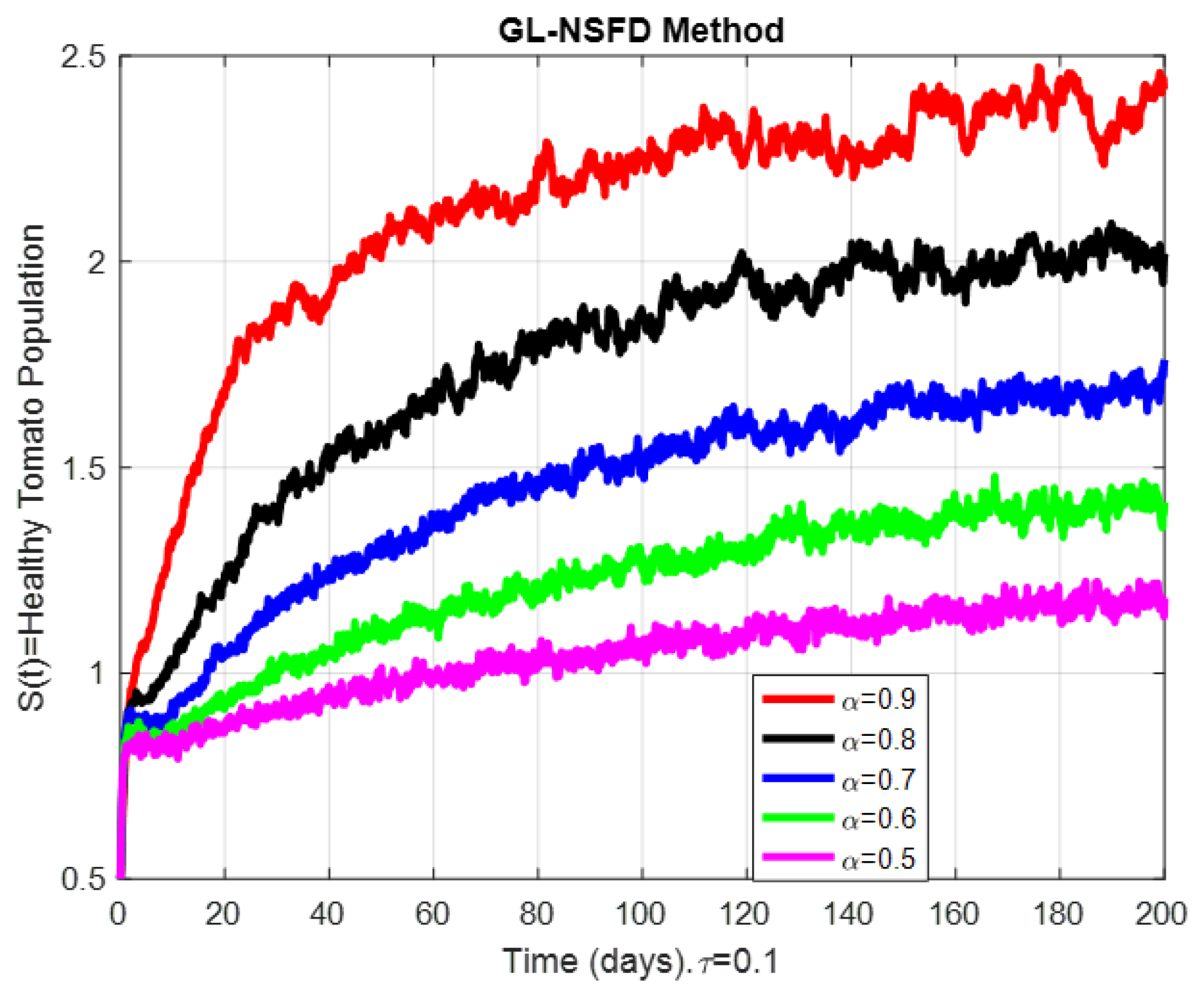
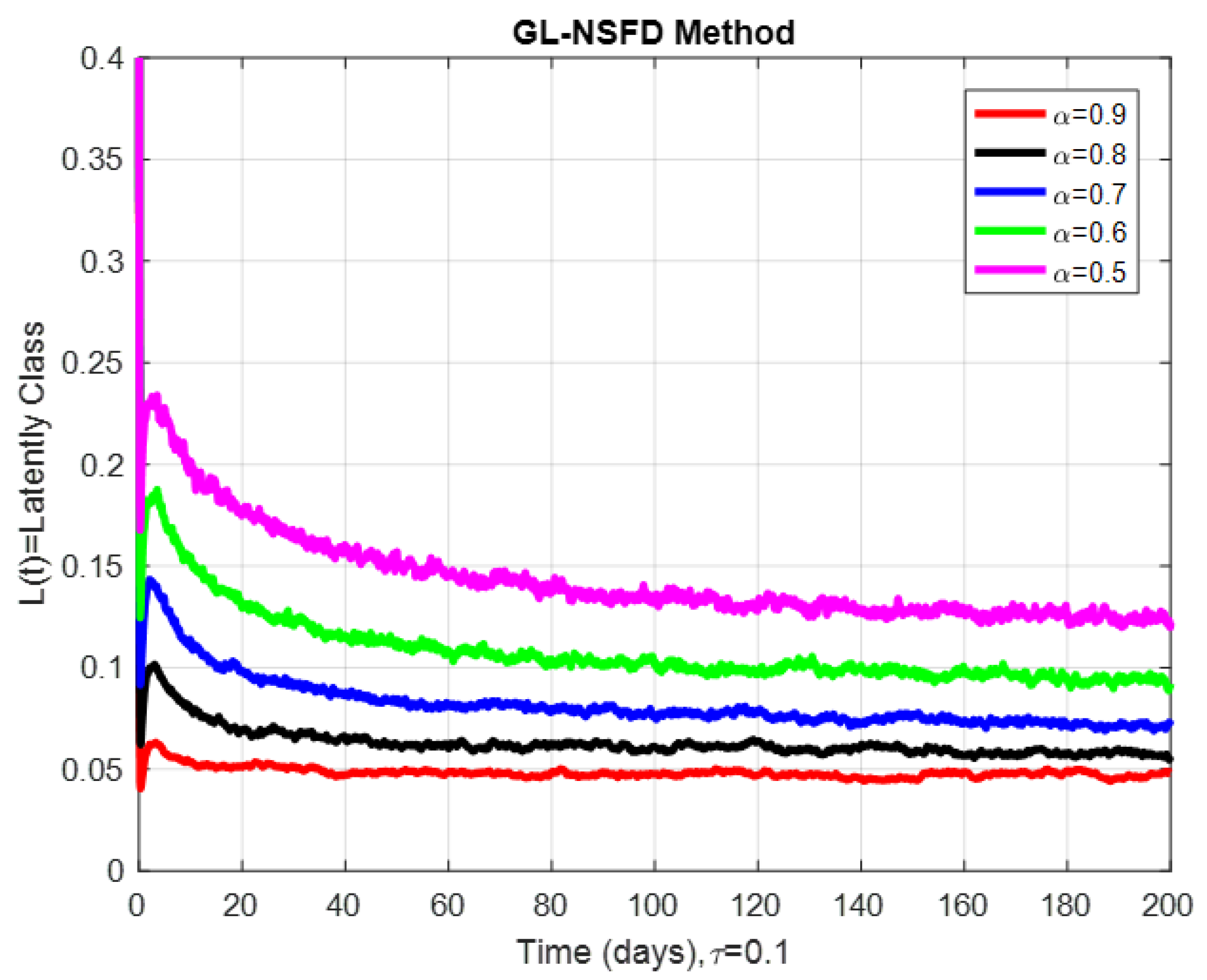
The behavior of TYLCV with dynamic activity under a stochastic delay fractional-order model was numerically simulated through the variation of the fractional order α { 0.5 , 0.6 , 0.7 , 0.8 , 0.9 } and a constant delay parameter τ = 0.1 . This shows the joint impact of memory effects and random disturbances on the spread of the disease through plant and vector populations. The solutions appear in terms of five major compartments: healthy tomatoes S ( t ) , latent tomatoes L ( t ) , infected tomatoes X ( t ) , healthy vectors E ( t ) , and infected vectors Y ( t ) . The dynamics of the healthy tomato population S ( t ) , as indicated by Figure 3, grow very rapidly as the fractional order ( α ) increases. For low values of ( α ) , representing more pronounced memory effects, the healthy population increases at a slower rate as a result of longer memory on the part of the system for infection states in the past. By contrast, for large values of ( α ) , especially as “ α 1 ”, the memory effect becomes weaker, enabling quicker recovery and stabilization of the healthy population. This means that recovery is delayed due to memory effects and will need to be considered in designing disease management strategies. In the latent tomato compartment L ( t ) , Figure 4 exhibits a decreasing trend across time. The decline, however, is more pronounced for greater ( α ) to signify a quicker transition away from the latent stage. When ( α ) is small, the memory of the system preserves the latent status for a longer duration, thus delaying transition into the infectious class. This stresses the fractional order’s role in controlling the latency period: the more intense the memory, the longer the system delay, and thus the longer the risk of outbreak. For the infected tomato population X ( t ) , higher values of ( α ) result in a higher rate of decline of infection number, while smaller values yield an ongoing or even increasing infected population, as illustrated in Figure 5, reflecting that at low ( α ) , the system retains past infection information more strongly, contributing to ongoing disease spread. This persistence suggests that fractional models may better capture the chronic nature of TYLCV epidemics, especially when recovery delays and infection event variability are significant. In the case of Figure 6, the healthy vector population E ( t ) , stability is evident at higher ( α ) with comparatively fewer oscillations. On the other hand, when ( α ) is smaller, the healthy vector population declines more dramatically because of greater infection pressure due to infected plants and the greater effect of memory on the transmission process. What this suggests is that environmental memory has an influence on how rapidly vectors become infected and how efficient they are in perpetuating disease transmission. Infected vector population Y ( t ) in Figure 7 follows behavior inversely related to that of healthy vectors. With small ( α ) , the infected vector population rises and oscillates more, sustaining high levels longer. As ( α ) grows, the infected vector population declines more quickly. This is potentially because of the diminished memory effect and faster ability of the system to adapt and shut down infection. These observations indicate that early intervention in vector control is of importance when memory effects are high and there are delays in disease detection or response. Therefore, the research indicates that the fractional order ( α ) and the stochastic delay component play highly significant roles in TYLCV dynamics. Smaller ( α ) values indicate systems with higher memory and delayed response, leading to more long-lasting and severe outbreaks. More ( α ) values, which approach classical integer-order models, result in faster stabilization and recovery. Therefore, the inclusion of fractional calculus and stochastic delay in epidemiological models is a more realistic model for describing and managing intricate plant–virus–vector interactions like that of TYLCV. Furthermore, the stochastic perturbations are interpreted in the Itô sense, reflecting random environmental fluctuations around the deterministic drift. The intensity ( σ i ) modulates noise amplitude for each compartment. Although analytical treatment of stochastic stability is beyond this paper’s scope, numerical experiments show that increasing ( σ i ) enhances solution variance and can induce random outbreak peaks even when ( R 0 < 1 ) .

10. Conclusions

This study introduces and investigates a non-integer mathematical framework for the transmission dynamics of TYLCD, formulated using the Caputo fractional derivative. The proposed model captures the essential epidemiological mechanisms that govern the spread of TYLCV. The properties of the model, such as existence, uniqueness, positivity, and boundedness, are rigorously studied. Equilibrium points of the model are determined, and the basic reproduction number R 0 is computed using the recently developed next-generation matrix method. A sensitivity analysis, carried out around R 0 , identifies the most sensitive parameters that have the largest impact on disease transmission. Employing the Lyapunov functional technique, both local and global asymptotic stability of equilibria are established, namely the disease-free equilibrium when R 0 < 1 and the endemic equilibrium when R 0 > 1 . Numerical experiments, using the Grünwald–Letnikov nonstandard finite difference (GL-NSFD) scheme, illustrate the significant role of fractional memory and time-delay interventions on disease spread. This suggests that fractional-order memory dynamics can improve the performance of controls against TYLCV. In future work, fractal–fractional derivatives will be considered in the Caputo sense to design an optimal control framework that improves accuracy and biological realism in the predictive modeling of plant viral epidemics.

Author Contributions

Conceptualization, A.R., M.L. and U.S.; Methodology, A.R., M.A. and U.S.; Software, A.R.; Validation, M.A., A.R., M.L. and E.G.R.; Formal analysis, A.R. and U.S.; Investigation, A.R.; Resources, A.R.; Data curation, A.R.; Writing—original draft, A.R. and U.S.; Writing—review & editing, M.A., A.R., M.L., U.S. and E.G.R.; Visualization, M.A., A.R. and M.L.; Supervision, A.R. and M.L.; Project administration, A.R. and M.L.; Funding acquisition, A.R. and E.G.R. All authors have read and agreed to the published version of the manuscript.

Funding

This work was supported by the Ministry of Education, Youth and Sports of the Czech Republic through the e-INFRA CZ (ID:90254), with the financial support of the European Union under the REFRESH—Research Excellence For Region Sustainability and High-tech Industries project number CZ.10.03.01/00/22-003/0000048 via the Operational Programme Just Transition, and by Grant of SGS No.SP2025/049, VŠB—Technical University of Ostrava, Czech Republic.

Data Availability Statement

The references for the data used to support the findings of this study are cited within the article.

Acknowledgments

Princess Nourah bint Abdulrahman University Researchers Supporting Project No. (PNURSP2025R895), Princess Nourah bint Abdulrahman University, Riyadh, Saudi Arabia.

Conflicts of Interest

The authors declare no conflict of interest.

References

  1. Hugo, A.; Lusekelo, E.M.; Kitengeso, R. Optimal control and cost effectiveness analysis of tomato yellow leaf curl virus disease epidemic model. Appl. Math. 2019, 9, 82–88. [Google Scholar]
  2. Mo, H.; Wei, L. Tomato yellow leaf curl virus detection based on cross-domain shared attention and enhanced BiFPN. Ecol. Inform. 2025, 85, 102912. [Google Scholar] [CrossRef]
  3. Hemmati, F.; Behjatnia, S.A.A.; Moghadam, A.; Afsharifar, A. Induction of systemic resistance against cucumber mosaic virus (CMV) and tomato yellow leaf curl virus (TYLCV) in tomato. Int. J. Pest Manag. 2025, 71, 307–320. [Google Scholar] [CrossRef]
  4. Wang, Z.; Gong, P.; Zhao, S.; Li, F.; Zhou, X. Functional Characterization of Dual-Initiation Codon-Derived V2 Proteins in Tomato Yellow Leaf Curl Virus. Agronomy 2025, 15, 1726. [Google Scholar] [CrossRef]
  5. Koeda, S.; Fortes, I.M.; Rodríguez-López, M.J.; Fernández-Muñoz, R.; Moriones, E. Resistance to the insect vector Bemisia tabaci enhances the robustness and durability of tomato yellow leaf curl virus resistance conferred by Ty-1. Plant Dis. 2025, 109, 399–409. [Google Scholar] [CrossRef]
  6. Kumar, M.; Bag, S.; McAvoy, T.; Torrance, T.; Cloud, C.; Simmons, A.M. A shift in begomovirus Coheni populations associated with tomato yellow leaf curl disease infecting tomato cultivars in the southeastern united States. Plant Pathol. 2025, 74, 1277–1289. [Google Scholar] [CrossRef]
  7. Xu, Y.; Zhang, T.; Mu, S.; Peng, Y.; Wu, D.; Yang, L.; Li, Q.; Wu, Z.; Zhang, J. Discovery of Arbutin as Novel Potential Antiviral Agent Against Tomato Yellow Leaf Curl Virus. J. Agric. Food Chem. 2025, 73, 3967–3976. [Google Scholar] [CrossRef]
  8. Li, P.; Zhang, L.; Yan, X.T.; Zheng, C.; Zhang, X.Y.; Chen, J.P.; Liu, S.S.; Wang, X.W. Suppression of TGA2-mediated Salicylic Acid Defence by Tomato Yellow Leaf Curl Virus C2 via Disruption of TCP7-like Transcription Factor Activity in Tobacco. Plant Cell Environ. 2025, 48, 4039–4050. [Google Scholar] [CrossRef]
  9. Brites, N.M.; Braumann, C.A. Profit Optimization of Stochastically Fluctuating Populations under Harvesting: The Effects of Allee Effects. Optimization 2022, 71, 3277–3293. [Google Scholar] [CrossRef]
  10. Salcedo-Varela, G.; Diaz-Infante, S. Threshold behaviour of a stochastic vector plant model for tomato yellow curl leaves disease: A study based on mathematical analysis and simulation. Int. J. Comput. Math. 2024, 101, 1430–1453. [Google Scholar] [CrossRef]
  11. Septiana, A.Z.; Mahfut, M.; Handayani, T.T.; Suratman. Survey of Tomato yellow leaf curl virus (TYLCV) infection on Solanum lycopersicum L. in Lampung, Indonesia. AIP Conf. Proc. 2024, 2970, 050027. [Google Scholar] [CrossRef]
  12. Al-Matroushi, A.R.; e Ammara, U.; Shahid, M.S.; Khan, J.; Al-Sadi, A.M. Genetic diversity and infectivity analysis of tomato yellow leaf curl virus Oman and its associated betasatellite. Cell. Mol. Biol. 2024, 70, 101–108. [Google Scholar] [CrossRef]
  13. Marchant, W.G.; Brown, J.K.; Gautam, S.; Ghosh, S.; Simmons, A.M.; Srinivasan, R. Non-feeding transmission modes of the tomato yellow leaf curl virus by the whitefly Bemisia tabaci do not contribute to reoccurring leaf curl outbreaks in tomato. Insects 2024, 15, 760. [Google Scholar] [CrossRef] [PubMed]
  14. Wei, Y.; Gao, L.; Zhang, Z.; Li, K.; Zhang, Z.; Zhang, D.; Chen, J.; Peng, J.; Gao, Y.; Du, J.; et al. D-limonene affects the feeding behavior and the acquisition and transmission of tomato yellow leaf curl virus by Bemisia tabaci. Viruses 2024, 16, 300. [Google Scholar] [CrossRef] [PubMed]
  15. Koeda, S.; Kitawaki, A. Breakdown of Ty-1-based resistance to tomato yellow leaf curl virus in tomato plants at high temperatures. Phytopathology 2024, 114, 294–303. [Google Scholar] [CrossRef] [PubMed]
  16. Gaertner, N.F.; Maio, F.; Arroyo-Mateos, M.; Luna, A.P.; Sabarit, B.; Kwaaitaal, M.; Eltschkner, S.; Prins, M.; Bejarano, E.R.; van den Burg, H.A. A SUMO interacting motif in the Replication initiator protein of Tomato yellow leaf curl virus is required for viral replication. bioRxiv 2024. [Google Scholar] [CrossRef]
  17. Wang, Y.M.; Xie, T.; He, Y.Z.; Cuellar, W.J.; Wang, X.W. Heat stress promotes the accumulation of tomato yellow leaf curl virus in its insect vector by activating heat shock factor. Crop Health 2024, 2, 19. [Google Scholar] [CrossRef]
  18. Sabbar, Y.; Aldosary, S.F. A general epidemic model with variable-order fractional derivatives and Lévy noise: Dynamical analysis and application to historical influenza data. Alex. Eng. J. 2025, 130, 459–482. [Google Scholar] [CrossRef]
  19. Petráš, I. Fractional-Order Nonlinear Systems: Modeling, Analysis and Simulation; Nonlinear Physical Science; Springer: Berlin/Heidelberg, Germany, 2011. [Google Scholar]
  20. Podlubny, I. Fractional Differential Equations: An Introduction to Fractional Derivatives, Fractional Differential Equations, to Methods of Their Solution and Some of Their Applications; Elsevier: Amsterdam, The Netherlands, 1998; Volume 198. [Google Scholar]
  21. Kilbas, A. Theory and Applications of Fractional Differential Equations; North-Holland Mathematics Studies; Elsevier: Amsterdam, The Netherlands, 2006; Volume 204. [Google Scholar]
  22. Li, Y.; Chen, Y.; Podlubny, I. Stability of fractional-order nonlinear dynamic systems: Lyapunov direct method and generalized Mittag–Leffler stability. Comput. Math. Appl. 2010, 59, 1810–1821. [Google Scholar] [CrossRef]
  23. Butter, N.; Rataul, H. The virus-vector relationship of the Tomato leafcurl virus (TLCV) and its vector, Bemisia tabaci Gennadius (Hemiptera: Aleyrodidae). Phytoparasitica 1977, 5, 173–186. [Google Scholar] [CrossRef]
  24. Li, K.; Turechek, B.W.; Adkins, S.; Luo, W.; Mellinger, H.C.; Smith, H.; Kousik, C.S.; Roberts, P.; Parks, F.; Lucas, L.; et al. Satellite-based Crop Identification and Risk Profiling for Area Wide Management of Whitefly and Tomato Yellow Leaf Curl Virus in Southwest Florida. Plant Dis. 2025. [Google Scholar] [CrossRef]
  25. Li, C.; Zhang, F. A survey on the stability of fractional differential equations: Dedicated to Prof. YS Chen on the Occasion of their 80th Birthday. Eur. Phys. J. Spec. Top. 2011, 193, 27–47. [Google Scholar] [CrossRef]
  26. Zamir, M.; Nadeem, F.; Abdeljawad, T.; Hammouch, Z. Threshold condition and non pharmaceutical interventions’s control strategies for elimination of COVID-19. Results Phys. 2021, 20, 103698. [Google Scholar] [CrossRef]
  27. Berhe, H.W.; Gebremeskel, A.A.; Melese, Z.T.; Al-arydah, M.; Gebremichael, A.A. Modeling and global stability analysis of COVID-19 dynamics with optimal control and cost-effectiveness analysis. Partial. Differ. Equ. Appl. Math. 2024, 11, 100843. [Google Scholar] [CrossRef]
  28. Chitnis, N.; Hyman, J.M.; Cushing, J.M. Determining important parameters in the spread of malaria through the sensitivity analysis of a mathematical model. Bull. Math. Biol. 2008, 70, 1272–1296. [Google Scholar] [CrossRef]
  29. Scherer, R.; Kalla, S.L.; Tang, Y.; Huang, J. The Grünwald–Letnikov method for fractional differential equations. Comput. Math. Appl. 2011, 62, 902–917. [Google Scholar] [CrossRef]
  30. Sweilam, N.; Nagy, A.; Elfahri, L. Nonstandard finite difference scheme for the fractional order Salmonella transmission model. J. Fract. Calc. Appl. 2019, 10, 197–212. [Google Scholar]
  31. Narasegowda Maruthi, M.; Czosnek, H.; Vidavski, F.; Tarba, S.Y.; Milo, J.; Leviatov, S.; Mallithimmaiah Venkatesh, H.; Seetharam Padmaja, A.; Subbappa Kulkarni, R.; Muniyappa, V. Comparison of resistance to Tomato leaf curl virus (India) and Tomato yellow leaf curl virus (Israel) among Lycopersicon wild species, breeding lines and hybrids. Eur. J. Plant Pathol. 2003, 109, 1–11. [Google Scholar] [CrossRef]
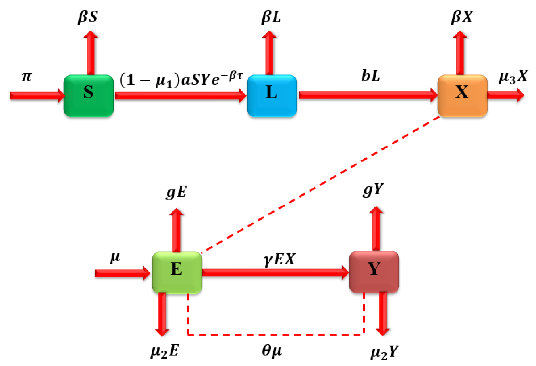
Figure 1. Flowchart of TYLCD.
Fractalfract 09 00754 g001
Figure 2. Normalized sensitivity indices of model parameters on the basic reproduction number R 0 .
Fractalfract 09 00754 g002
Figure 3. Variation in healthy tomato dynamics with fractional order α .
Fractalfract 09 00754 g003
Figure 4. Variation in latent class dynamics with fractional order α .
Fractalfract 09 00754 g004
Figure 5. Variation of infectious tomato plant dynamics with fractional order α .
Fractalfract 09 00754 g005
Figure 6. Variation of vector population with fractional order α .
Fractalfract 09 00754 g006
Figure 7. Variation in infective vector dynamics with fractional order α .
Fractalfract 09 00754 g007
Table 1. Model parameters, their description, and experimental basis.
ParameterDescriptionExperimental Basis/Reference
π Rate at which healthy tomato plants are introduced into the fieldAssumed
β Constant removal rate of all plant classes due to the fixed crop cycle duration[1]
aRate at which healthy plants become latently infected due to contact with infective vectors[5,14]
bRate at which latently infected plants become infectious (inverse of mean latent period)[3,15]
γ Rate at which non-infective vectors acquire infection from infectious plants[23]
μ Constant rate of incoming vectors from external sourcesAssumed
θ Fraction of immigrating vectors that are infective[1]
gNatural death rate of the vector population[5]
μ 1 Intensity of protective netting to reduce vector immigration[1]
μ 2 Intensity of insecticide spraying to decrease vector abundance[24]
μ 3 Intensity of infected plant removal and safe disposal measures[1]
Table 2. Normalized (elasticity) sensitivity indices of R 0 evaluated at the baseline parameter values (with a ±10% perturbation range).
ParameterValueSensitivity Index Υ p
π α 0.5 1 2 > 0
b α 0.4348 β α 2 ( b α + β α ) > 0
γ α 0.5 1 2 > 0
μ α 0.5 1 2 > 0
a α 0.5 1 2 > 0
θ α −0.125 θ α 2 ( 1 θ α ) < 0
β α −0.10437 α 2 1 + β α τ + β α b α + β α + β α β α + μ 3 α < 0
μ 1 α −0.0555 μ 1 α 2 ( 1 μ 1 α ) < 0
g α −0.2727 g α 2 ( g α + μ 2 α ) < 0
μ 2 α −0.2727 g α 2 ( g α + μ 2 α ) < 0
μ 3 α −0.083 μ 3 α 2 ( β α + μ 3 α ) < 0
Table 3. Parameters and values of the model.
ParametersValues (day−1)Reference
π α 0.5Assumed
β α 0.5Assumed
a α 1.01Assumed
b α 0.075[1]
γ α 0.003[23]
μ α 0.3[31]
θ α 0.2[31]
g α 0.06[1]
μ 1 α 0.1[1]
μ 2 α 0.5[1]
μ 3 α 0.1[1]
σ i 0 σ i 1 Assumed
Disclaimer/Publisher’s Note: The statements, opinions and data contained in all publications are solely those of the individual author(s) and contributor(s) and not of MDPI and/or the editor(s). MDPI and/or the editor(s) disclaim responsibility for any injury to people or property resulting from any ideas, methods, instructions or products referred to in the content.