Article

Dynamic Analysis of a Fractional-Order Model for Vector-Borne Diseases on Bipartite Networks

by
Weiyi Xu
1,
Zhenzhen Lu
2,
Chengyi Wang
1,
Yuxuan Han
1 and
Yongguang Yu
1,*
1
School of Mathematics and Statistics, Beijing Jiaotong University, Beijing 100044, China
2
School of Mathematical Sciences, Inner Mongolia University, Hohhot 010021, China
*
Author to whom correspondence should be addressed.
Fractal Fract. 2025, 9(11), 742; https://doi.org/10.3390/fractalfract9110742 (registering DOI)
Submission received: 24 September 2025 / Revised: 5 November 2025 / Accepted: 11 November 2025 / Published: 17 November 2025

Abstract

Vector-borne infectious diseases transmitted by vector organisms (e.g., mosquitoes, rodents, and ticks) are recognized as key priorities in global public health. The construction of host–vector interaction frameworks within bipartite networks enables a clearer depiction of the transmission mechanisms underlying vector-borne infectious diseases. Compared with traditional models, the effective influence of historical information on vector-borne infectious diseases is more critical. In this study, the long-term memory behavior of infected populations during the recovery phase is regarded as a power-law tail distribution, a result that is consistent with fractional calculus. Thus, a fractional-order model for vector-borne diseases on bipartite networks is established.The basic reproduction number is derived about network topology and fractional order. With stability analysis, the conditions governing the global extinction and global persistence of vector-borne infectious diseases are determined. Furthermore, the validity of the proposed model is confirmed through numerical simulation results obtained from Barabási–Albert (BA) networks and Watts–Strogatz (WS) networks.

1. Introduction

Vector-borne diseases pose a significant threat to public health worldwide. The World Health Organization (WHO) estimates that millions of people die from vector-borne diseases each year. These diseases not only impose a huge health burden, but also have a particularly severe impact on developing countries, potentially leading to poverty and development setbacks. Common vector-borne infectious diseases include malaria, dengue fever, and Zika virus, as well as some diseases transmitted by plague and ticks. Explaining the prevalence and development of vector-borne infectious diseases among the population from a mathematical perspective is a highly significant and rational approach. The evolution of mathematical modeling for vector-borne diseases has witnessed a series of significant advancements. Early frameworks, such as the Ross–Macdonald model in 1911 [1] established the foundational framework for studying malaria transmission by integrating human and vector populations through a mass-action formulation [1].
d x ( t ) d t = γ x ( t ) a b m [ 1 x ( t ) ] y ( t ) , d y ( t ) d t = μ y ( t ) a c [ 1 y ( t ) ] x ( t ) .
This model separated the transmission dynamics into two compartments: human hosts x ( t ) and female Anopheles mosquitoes y ( t ) , with parameters representing infection probabilities γ , mortality rates μ , a is the biting rate on humans by a single vector, b is the probability of infective bites on a human that produce an infection, c is the probability of infective bites that produce an infective vector, and m represents the average number of mosquitoes each person possesses. Since then, many researchers have paid more attention to building a framework of mathematical models to study vector-borne diseases including Dengue Fever, Rift Valley Fever, West Nile Fever, etc. [2,3,4,5,6,7]. These studies refine the quantification of transmission dynamics based on foundational frameworks. They move beyond the system (1) to more accurately capture the interaction between human hosts and vector populations, extend mathematical modeling from malaria to other vector-borne diseases, and improve the interpretability of model outputs for real-world public health decisions.
Traditional models oversimplified the intricate interactions between hosts and vectors—a limitation that hindered accurate analysis of vector-borne disease dynamics. Among the diverse array of complex networks, bipartite network models have stood out as an essential tool for investigating vector-borne diseases. Bipartite network models explicitly depict the bipartite interactions between hosts and vectors that form the very foundation of vector-borne disease transmission dynamics in networks. Over the past few decades, numerous scholars have built on the foundation of bipartite network models to conduct in-depth studies on vector-borne diseases. Focusing on complex networks, Masuda developed multi-state epidemic models in 2006. A core insight from his work was the emphasis on the network heterogeneity’s crucial role in models with competing pathogens—specifically, that pathogen co-existence relies not only on heterogeneous contact rates but also on network-independent conditions [8]. Research into vector-borne disease spread on bipartite networks was led by Bisanzio in 2010, and his work broke new ground by proving that scale-free degree distributions cause epidemic thresholds to vanish [9]. The global dynamics of vector-borne diseases on bipartite networks became the focus of Zhang’s 2020 study [10], In 2011, Tanimoto introduced immunization strategies in bipartite network models, with the innovation of targeted immunization and studying the effect of immunization rates on reducing epidemic thresholds for diseases like STDs [11]. In 2013, Hernandez presented a deeper analysis of epidemic thresholds for bipartite networks, revealing the existence of critical infectivity values for each population to prevent epidemics [12]. In 2015, Zhang introduced a delayed SIS model to study the impact of incubation periods for both humans and vectors, exploring how time delays affected the basic reproduction number and disease spread dynamics [13]. which built on and extended earlier models. A key finding from this research was that degree distribution heterogeneity accelerates disease transmission [10]. In 2021, Zhao’s [14] contribution to bipartite network modeling involved adding two time delays to the framework. By making this adjustment, he was able to explore how double time delays influence both the basic reproduction number and its global stability [14]. These studies further confirm that integrating complex network theory into vector-borne disease mathematical modeling is not just a scientific advancement, but a necessary innovation to overcome the inherent limitations of traditional approaches. This integration not only deepens the understanding of disease transmission mechanisms that traditional models could not unravel but also paves the way for developing more targeted and effective control measures, making it essential for bridging the gap between theoretical modeling and real-world public health practice.
Furthermore, traditional differential equation models often fall short in capturing the time-lagged and memory effects that are deeply ingrained in biological and social systems. For instance, the life cycle of disease carrying vectors, such as mosquitoes in the case of malaria or dengue, and the subsequent spread of the disease are influenced by complex temporal patterns and memory-based factors. Fractional calculus, however, presents a highly potent mathematical instrument for depicting these nonlocal processes. It allows for a more precise representation of delayed and memory dependent phenomena [15,16,17,18]. By integrating fractional derivatives into disease transmission models, researchers can gain a more comprehensive understanding of the temporal dynamics of infection. This, in turn, significantly improves the accuracy of predictions. Angstmann et al. posited that the fractional-order SIR model stemmed from an underlying physical random process [19,20,21]. They broadened the application of the power-law distribution to incorporate the Mittag-Leffler distribution, thereby developing a model rooted in fractional calculus. The resulting right-hand-side differential equation for the Riemann–Liouville fractional-order derivative diverged from existing fractional-order epidemic models. These investigations highlighted that a key method for constructing such fractional-order models involved considering the continuous time random walk (CTRW) process and the power-law distribution waiting time. Crucially, no prior models combined power-law distribution waiting times with bipartite network interactions to study vector-borne diseases, leaving a critical gap in integrating nonlocal temporal dynamics and real-world network structures. To address this gap, this paper establishes a fractional-order model for vector-borne diseases, a necessary CTRW fractional modeling innovation: it captures vector-borne disease systems’ long-term recovery capabilities and fills the void of linking CTRW-derived fractional dynamics to bipartite networks, enabling more realistic, accurate vector-borne disease system analysis.
In order to elucidate the potential mechanisms of the transmission of vector-borne diseases in a bipartite network environment, this paper constructs a fractional-order infectious disease model based on the bipartite network. With a particular emphasis on the impacts of network topology and fractional-order on the two types of equilibrium points of vector-borne diseases, we also analyze the effect of the basic reproduction number R 0 on the long term behavior of the model. Numerical simulations support the theoretical analysis for given parameter values. The main contributions of this study are as follows:
(i)
The long-memory behavior of the infected population during the recovery period is represented by a power-law tail distribution and described using an α -order Riemann–Liouville fractional integral.
(ii)
Using the unique topology of bipartite networks, the model of the basic reproduction number with fractional-order effects is derived. As a critical threshold, it differentiates the stability regions of disease-free and endemic equilibrium points, and defines the conditions of the stability in the model.
(iii)
Using scale-free and small-world networks as case studies, simulation results aligning with theoretical findings are derived, which furnish evidence for relevant models in complex networks.
The rest of this paper is structured as below. In Section 2, some preliminaries about the fractional-order calculus are given, then a fractional-order model for vector-borne diseases on bipartite networks is built. In Section 3, Some qualitative properties of the fractional-order model are discussed. Moreover, some numerical simulations are given to verify the theoretical results in Section 4. Finally, conclusions are discussed in Section 5.

2. Preliminaries and Problem Formulation

2.1. Preliminaries

This section begins with some definitions and results.
Definition 1.
A Gamma function of α is defined by:
Γ ( α ) = 0 t α 1 e t d t , t t 0 ,
where α C , [ α ] > 0 .
Definition 2.
The α-order ( α > 0 ) Riemann–Liouville (R-L) fractional integral of a function f ( t ) is defined by
I t α t 0 f ( t ) = 1 Γ ( α ) t 0 t ( t s ) α 1 f ( s ) d s , t t 0 .
Definition 3.
The α-order ( α > 0 ) R-L fractional derivative of a function f ( t ) is defined by
D t α t 0 R f ( t ) = d n d t n I t n α t 0 f ( t ) , t t 0 ,
where n = [ α ] + 1 .
Definition 4.
Let g ( t ) be the function about time t and g ( t ) = 0 when t < 0 ; s is a complex variable. The Laplace transform and the inverse Laplace transform of f are defined by
G ( s ) = L t { g ( t ) } = 0 g ( t ) e s t d t , g ( t ) = L s { G ( s ) } = 1 2 π i β i β + i G ( s ) e s t d s ,
when g ( t ) = 0 D t α f ( t ) in Definition (2), the Laplace transform of the Riemann–Liouville fractional integral is given by
L t { 0 D t α f ( t ) } = s α L t f ( t ) .
Lemma 1.
([22]). Suppose that a function f : R + R is twice differentiable and that f ̲ < f ¯ . Then, there are sequences ( t n ) and ( τ n ) as n such that
f ( t n ) f ̲ , f ( t n ) = 0 , f ( t n ) 0 ,
and
f ( τ n ) f ¯ , f ( τ n ) = 0 , f ( τ n ) 0 .
Lemma 2.
([23] (Poincaré–Bendixson property)). Let Ω be a non-empty, closed, and bounded limit set of a dynamical system, and suppose that Ω contains no equilibrium points. Then, Ω is a closed orbit.
Lemma 3.
([24,25]). Assume that
  • (H1) D is simply connected, where D R n ;
  • (H2) There is a compact absorbing set K D ;
  • (H3) The dynamical system satisfies the Poincaré–Bendixson property;
  • (H4) X * is a unique equilibrium point of the dynamical system in D provided it is stable.
Then the equilibrium point X * of the dynamical system is globally asymptotically stable in D.

2.2. Survival Probability in the Recovery Process

To derive the dynamic equation of the fractional-order SIS-SI model, we first describe the counting process of the infected compartment I k H ( t ) changing over time. Let P ( t ) denote the probability that no event (i.e., no recovery event) has occurred by time t; in other words, it represents the probability that an individual remains in the infected state at least until time t. The number of individuals in the I k H ( t ) compartment at time t can be expressed as,
I k H ( t ) = 0 t β M H k S k H ( τ ) Θ ( I M ) e μ ( t τ ) d τ 0 t γ I k H ( τ ) P ( t τ ) e μ ( t τ ) d τ ,
where P ( 0 ) = 0 ; then, differentiate Equation (3) to produce
d I k H ( t ) d t = β M H k S k H ( t ) Θ ( I M ) μ 0 t β M H k S k H ( τ ) Θ ( I M ) e μ ( t τ ) d τ γ I k H ( t ) P ( 0 ) γ 0 t I k H ( x ) P ( t τ ) e μ ( t τ ) d τ + γ μ 0 t I k H ( τ ) P ( t τ ) e μ ( t τ ) d τ , = β M H k S k H ( t ) Θ ( I M ) μ I k H ( t ) γ 0 t I k H ( τ ) P ( t τ ) e μ ( t τ ) d τ .
Empirical studies [26,27,28,29,30,31,32,33,34] have demonstrated that in a wide range of real-world scenarios, the inter-event time distribution exhibits heavy-tailed characteristics, frequently conforming to a power law distribution. Such distributions emerge in human activity patterns, social interactions, and biological processes—attributes rendering them highly pertinent for modeling disease recovery dynamics. Consequently, in the present study, the power law distribution is adopted as an illustrative example. Let P ( t ) = t α Γ ( α + 1 ) , P ( t ) = t α 1 Γ ( α ) ; then
0 t I k H ( τ ) P ( t τ ) e μ ( t τ ) d τ = e μ t L t { I k H ( t ) e μ t } L t { P ( t ) } , = e μ t L t { I k H ( t ) e μ t } [ s L t { P ( t ) } P ( 0 ) ] , = e μ t L t { I k H ( t ) e μ t } s α .
According to the properties of the Riemann–Liouville fractional-order integral,
d I k H ( t ) d t = β M H k S k H ( t ) Θ ( I M ) μ I k H ( t ) γ exp ( μ t ) 0 D t α ( I k H ( t ) exp ( μ t ) ) .

2.3. Dynamic Equations of the Fractional-Oder SIS-SI Model on Bipartite Networks

In this subsection, the mean-field equations of the fractional-order SIS-SI model are systematically derived, with the explicit assumption that vector-borne diseases (e.g., malaria and dengue fever, which rely on intermediate vectors like mosquitoes for transmission) spread over a well-defined bipartite network. The bipartite network structure is shown in Figure 1.
The average degree of the host network (comprising the population of organisms susceptible to and infected by the disease, such as humans in mosquito-borne disease models) within the complex system is uniformly denoted as k , and the average degree of the vector network (consisting of the intermediate carriers that transmit the disease, e.g., mosquitoes, ticks) as l . Based on the above discussion, the fractional-order model is as follows:
d S k H ( t ) d t = μ β M H k S k H ( t ) Θ ( I M ) + γ exp ( μ t ) 0 D t α ( I k H ( t ) exp ( μ t ) ) μ S k H ( t ) , d I k H ( t ) d t = β M H k S k H ( t ) Θ ( I M ) γ exp ( μ t ) 0 D t α ( I k H ( t ) exp ( μ t ) ) μ I k H ( t ) , d S l M ( t ) d t = μ ˜ β H M l S l M ( t ) Θ ( I H ) μ ˜ S l M ( t ) , d I l M ( t ) d t = β H M l S l M ( t ) Θ ( I H ) μ ˜ I l M ( t ) ,
where Θ ( I H ) = k = 1 n k p ( k ) I k H k , Θ ( I M ) = l = 1 m l p ( l ) I l M l . We assume the human recovered rate is denoted by γ . The human inflow rate is equal to the human mortality rate, denoted by μ . This assumption aims to simplify the model by ensuring the stability of human size over time. And the birth rate of vectors is equal to the mortality rate of vectors, denoted by μ ˜ . For short-lived vectors like mosquitoes, such simplification makes the model more analytically tractable, allowing a focused analysis of disease transmission dynamics without the need to account for the complexity introduced by population size fluctuations.

3. Model Analysis

In this section, the basic reproduction number R 0 will be formally derived. Guided by stability theory, the stability of the system (7) at both disease-free and endemic equilibrium points will be systematically analyzed.

3.1. Boundedness and Non-Negative of Solutions, the Basic Reproduction Number

Prior to investigating the stability, it is of great necessity to prove the boundedness and non-negative of the biological system.
Theorem 1.
If any solution of system (7) satisfies the inital condition, then all solutions are bounded and non-negative for t > 0 .
Proof. 
To investigate the non-negativity of the system, we consider the following system:
d S ˜ k H ( t ) d t = β M H k S ˜ k H ( t ) Θ ( I ˜ M ) + γ exp ( μ t ) 0 D t α ( I ˜ k H ( t ) exp ( μ t ) ) μ S ˜ k H ( t ) , d I ˜ k H ( t ) d t = β M H k S ˜ k H ( t ) Θ ( I ˜ M ) γ exp ( μ t ) 0 D t α ( I ˜ k H ( t ) exp ( μ t ) ) μ I ˜ k H ( t ) , d S ˜ l M ( t ) d t = β H M l S ˜ l M ( t ) Θ ( I ˜ H ) μ ˜ S ˜ l M ( t ) , d I ˜ l M ( t ) d t = β H M l S ˜ l M ( t ) Θ ( I ˜ H ) μ ˜ I ˜ l M ( t ) ,
where the initial conditions satisfy S ˜ k H ( 0 ) = 0 , I ˜ k H ( 0 ) = 0 , S ˜ l M ( 0 ) = 0 , I ˜ l M ( 0 ) = 0 . Apparently, ( 0 , 0 , 0 , 0 ) is the unique solution of the system (8). According to the comparison theorem, one can deduce that the solutions of the system (7) satisfy S k H ( t ) 0 , I k H ( t ) 0 , S l M ( t ) 0 , I l M ( t ) 0 .
About boundedness, one has
N H ( t ) = S k H ( t ) + I k H ( t ) = 1 , N M ( t ) = S l M ( t ) + I l M ( t ) = 1 .
That implies N H ( t ) , N M ( t ) is bounded, and the same as S k H ( t ) , I k H ( t ) , S l M ( t ) , I l M ( t ) . □
From Theorem 1 and the normalization condition (9), the following Ω is the positive invariant set for the system (7), as follows:
Ω = { ( S k H , I k H , S 1 m , I l m ) R + 2 n + 2 m : 0 S k H , I k H , 1 , k = 1 , 2 , , n , 0 S l m , I l m 1 , l = 1 , 2 , , m . }
Now, we consider the dynamics of the system (7) on the region Ω . Here, it can be found that S k H ( t ) + I k H ( t ) = 1 , S l M ( t ) + I l M ( t ) = 1 . Hence, we shall focus our attention on the following rewritten system:
d I k H ( t ) d t = β M H k ( 1 I k H ( t ) ) Θ ( I M ) γ exp ( μ t ) 0 D t α ( I k H ( t ) exp ( μ t ) ) μ I k H ( t ) , d I l M ( t ) d t = β H M l ( 1 I l M ( t ) ) Θ ( I H ) μ ˜ I l M ( t ) .
It is obvious that the equilibrium point state of the system (10) is defined by
lim t I k H ( t ) = I k H * , lim t I l M ( t ) = I l M * , lim t Θ ( I H ) = Θ ( I H * ) , lim t Θ ( I M ) = Θ ( I M * ) .
Splitting the remaining limit and based on the result of [20], one has
lim t γ e μ t D t α 0 ( I k H ( t ) e μ t ) = γ ( lim t e μ t D t α 0 ( e μ t I k H ( t ) ) ) , = γ μ α I k H * .
Then the equilibrium point state of the system (10) is satisfied by following equations:
0 = β M H k ( 1 I k H * ) Θ ( I M * ) γ μ α I k H * μ I k H * , k = 1 , 2 , , n , 0 = β H M l ( 1 I l M * ) Θ ( I H * ) μ ˜ I l M * , l = 1 , 2 , , l .
From (11),
I k H * = β M H k l = 1 m l p ( l ) β H M l Θ ( I H * ) β H M l Θ ( I H * ) + μ ˜ l β M H k l = 1 m l p ( l ) β H M l Θ ( I H * ) β H M l Θ ( I H * ) + μ ˜ l + γ μ α + μ , k = 1 , 2 , , n ,
substituting (12) into Θ ( I H * ) , then
Θ ( I H * ) = 1 k k = 1 n k 2 p ( k ) β M H l = 1 m l p ( l ) β H M l Θ ( I H * ) β H M l Θ ( I H * ) + μ ˜ β M H k l = 1 m l p ( l ) β H M l Θ ( I H * ) β H M l Θ ( I H * ) + μ ˜ + l ( γ μ α + μ ) f ( Θ ( I H * ) ) .
It is clear that the self-consistency Equation (13) has the solution Θ ( I H * ) = 0 . This means that the system (10) has a disease-free equilibrium point E 0 . Upon further differentiation of f ( Θ ( I H * ) ) , we have
f ( Θ ( I H * ) ) = 1 k k = 1 n k 2 p ( k ) β M H l ( γ μ α + μ ) f 1 ( Θ ( I H * ) ) ( f 2 ( Θ ( I H * ) ) ) 2 > 0 ,
where
f 1 ( Θ ( I H * ) ) = l = 1 m l p ( l ) β H M l μ ˜ ( β H M l Θ ( I H * ) + μ ˜ ) 2 , f 2 ( Θ ( I H * ) ) = β M H k l = 1 m l p ( l ) β H M l Θ ( I H * ) β H M l Θ ( I H * ) + μ ˜ + l ( γ μ α + μ ) .
Then f 2 ( Θ ( I H * ) ) > 0 , f 1 ( Θ ( I H * ) ) f 2 2 ( Θ ( I H * ) ) < 0 and f 1 ( Θ ( I H * ) ) f 2 ( Θ ( I H * ) ) > 0 . Due to
f ( Θ ( I H * ) ) = 1 k k = 1 n k 2 p ( k ) β M H l ( γ μ α + μ ) [ f 1 ( Θ ( I H * ) ) f 2 ( Θ ( I H * ) ) 2 f 1 ( Θ ( I H * ) ) f 2 ( Θ ( I H * ) ) ] ( f 2 ( Θ ( I H * ) ) ) 3 ,
we have f 2 ( Θ ( I H * ) ) < 0 , so Θ ( I H * ) is a rigorously increasing concave function. Because f ( 0 ) = 0 and f ( 1 ) < 1 , the self-consistency Equation (13) allows a unique nontrivial solution Θ ( I H * ) > 0 ( Θ ( I H * ) ( 0 , 1 ] ) only if
d f ( Θ ( I H * ) ) d Θ ( I H * ) Θ ( I H * ) = 0 = β M H β H M k 2 l 2 k l μ ˜ ( γ μ α + μ ) > 1 ,
where k 2 = k = 1 n k 2 p ( k ) , l 2 = l = 1 m l 2 p ( l ) .
Therefore, we define the basic reproduction number as follows
R 0 = β M H β H M k 2 l 2 k l μ ˜ ( γ μ α + μ ) .
Summarizing the above analysis, if R 0 > 1 , the system (10) has a unique epidemic equilibrium point E * .
Remark 1.
Notably, it becomes evident that the basic reproduction number we have obtained does contain the parameter α. This inclusion of α is not accidental but rather a direct reflection of the long memory considered for recovery rates in the model structure.

3.2. Stability Analysis

In this subsection, the stability analysis of the system (7) will be discussed, with a specific focus on analyzing the local stability and global stability of both the disease-free equilibrium point E 0 and the endemic equilibrium E * under different conditions of the basic reproduction number R 0 .
Theorem 2.
For the model (10),
(i) 
If R 0 < 1 , it has a unique disease-free equilibrium point E 0 = ( 0 , 0 ) which is locally asymptotically stable;
(ii) 
If R 0 = 1 , the disease-free equilibrium point E 0 is neutrally stable;
(iii) 
If R 0 > 1 , the disease-free equilibrium point E 0 is unstable, and the endemic equilibrium point E * is locally asymptotically stable.
Proof. 
The linearized system of (10) at the equilibrium E 0 is
d I k H ( t ) d t = β M H k Θ ( I M ) γ e 0 μ t D t α ( I k H ( t ) e μ t ) μ I k H ( t ) , d I l M ( t ) d t = β H M l Θ ( I H ) μ ˜ I l M ( t ) .
The Jacobian matrix at the disease-free equilibrium E 0 of the system (10) is
J 1 = A 11 A 12 A 21 A 22 ,
where
A 11 = γ μ α μ 0 0 0 0 γ μ α μ 0 0 0 0 γ μ α μ 0 0 0 0 0 γ μ α μ n × n ,
A 12 = β M H l p ( 1 ) β M H l 2 p ( 2 ) β M H l m p ( m ) 2 β M H l p ( 1 ) 2 β M H l 2 p ( 2 ) 2 β M H l m p ( m ) n β M H l p ( 1 ) n β M H l 2 p ( 2 ) n β M H l m p ( m ) n × m ,
A 21 = β H M k p ( 1 ) β H M k 2 p ( 2 ) β H M k n p ( m ) 2 β H M k p ( 1 ) 2 β H M k 2 p ( 2 ) 2 β H M k n p ( m ) m β H M k p ( 1 ) m β H M k 2 p ( 2 ) m β H M l n p ( m ) m × n ,
A 22 = μ ˜ 0 0 0 0 μ ˜ 0 0 0 0 μ ˜ 0 0 0 0 0 μ ˜ m × m ,
So the associated characteristic equation of the linearized system of (10) at the equilibrium point E 0 is
F ( λ ) = | λ I A | = ( λ + γ μ α + μ ) n 1 ( λ + μ ˜ ) m 1 [ λ 2 + ( μ ˜ + μ + γ μ α ) λ + μ ˜ ( μ + γ μ α ) β M H β H M k 2 l 2 k l ] .
Then we can discuss the stability of the disease-free equilibrium point E 0 . We need to verify that the eigenvalues of J 1 are negative; it is easy to see that n 1 eigenvalues of the characteristic equation are γ μ α μ and m 1 eigenvalues of the characteristic equation are all μ ˜ .
Assume the other two eigenvalues are λ 1 and λ 2 ; then λ 1 and λ 2 satisfy
λ 1 + λ 2 = ( μ ˜ + μ + γ μ α ) ,
and
λ 1 λ 2 = μ ˜ ( μ + γ μ α ) β M H β H M k 2 l 2 k l .
To discuss the distribution of all the eigenvalues, we consider three cases.
(i)
If R 0 < 1 , we have μ ˜ ( μ + γ μ α ) > β M H β H M k 2 l 2 k l . All eigenvalues of the characteristic Equation (10) are negative. Therefore E 0 = ( 0 , 0 ) is locally asymptotically stable.
(ii)
If R 0 = 1 , we have μ ˜ ( μ + γ μ α ) = β M H β H M k 2 l 2 k l , since λ = 0 is only a simple root of (10). Therefore E 0 is neutrally stable.
(iii)
If R 0 > 1 , we have μ ˜ ( μ + γ μ α ) < β M H β H M k 2 l 2 k l . Eigenvalues of the characteristic Equation (10) have a positive root. Therefore E 0 is unstable. And the endemic equilibrium point E * is locally asymptotically stable [10].
Theorem 3.
If R 0 < 1 , the system (10) has a unique disease-free equilibrium point E 0 = ( 0 , 0 ) and it is globally asymptotically stable.
Proof. 
According to Theorem 2, it has been known that if R 0 < 1 , the disease-free equilibrium point E 0 is locally asymptotically stable. To this end, we must now only to show that it is globally attractive. Note that system (10) is bounded, that is, I k H ( t ) , I l M ( t ) ( 0 , 1 ) . Then denote I k = lim sup t I k H ( t ) , I l = lim sup t I l M ( t ) . So I k and I l exist with 0 I k 1 and 0 I l 1 . By Lemma 1, there exists a sequence t n with t n as n such that I k H ( t n ) I k , I l M ( t n ) I l and I ˙ k H ( t n ) 0 ( n ) , I ˙ l M ( t n ) 0 ( n ) . The system (10) can be rewritten as
d I k H ( t n ) d t = β M H k ( 1 I k H ( t n ) ) Θ ( I M ( t n ) ) γ exp ( μ t n ) 0 D t α ( I k H ( t n ) exp ( μ t n ) ) μ I k H ( t n ) , d I l M ( t n ) d t = β H M l ( 1 I l M ( t n ) ) Θ ( I H ( t n ) ) μ ˜ I l M ( t n ) .
Take the limit of both sides of the above equations; one has
β M H k Θ ( I l ) = β M H k I k Θ ( I l ) + ( γ μ α + μ ) I k , β H M l Θ ( I k ) = β H M l I l Θ ( I k ) + μ ˜ I l .
If Θ ( I l ) > 0 , Θ ( I k ) > 0 and R 0 < 1 , the above equality yields
Θ ( I l ) = I k Θ ( I l ) + ( γ μ α + μ ) β M H k I k , = ( γ μ α + μ ) I k β M H k ( 1 I k ) , ( γ μ α + μ ) β M H k ( 1 I k ) , = R 0 k l ( γ μ α + μ ) 2 β M H 2 β H M k 2 l 2 k ( 1 I k ) ,
substituting I k = β M H k Θ ( I l ) β M H k Θ ( I l ) + γ μ α + μ into (20), we have
Θ ( I l ) R 0 k l ( γ μ α + μ ) 2 β M H 2 β H M k 2 l 2 k β M H k R 0 k l ( γ μ α + μ ) , < k l ( γ μ α + μ ) 2 β M H 2 β H M k 2 l 2 k β M H k k l ( γ μ α + μ ) , = γ μ α + μ β M H k ( R 0 1 ) .
On the other hand, Θ ( I l ) > 0 . This is a contradiction. So it can be concluded I l = 0 , that is, I l M ( t ) 0 . Similarly, it can be proved that I k H ( t ) 0 . Therefore, the disease-free equilibrium point E 0 is globally asymptotically stable when R 0 < 1 . □
Theorem 4.
If R 0 > 1 , the system (10) has a unique endemic equilibrium point E * = ( I k * , I l * ) and it is globally asymptotically stable.
Proof. 
It can be seen that T ˜ is simply connected and (H1) holds.
A compact absorbing set in T ˜ is equivalent to system (10) being uniformly persistent. Notably, the boundary T ˜ is a positive invariant of the system (10), in which there is the disease-free equilibrium point E 0 = ( 0 , 0 ) . By [35], we can conclude that the system (10) is uniformly persistent if R 0 > 1 . Thus, T ˜ is a compact absorbing set in T ˜ , satisfying (H2).
To verify (H3), let Ω be an omega limit set of (10) in T ˜ . If Ω excludes E * , Lemma 2 implies that Ω is a closed orbit. If Ω includes E * , Theorem 2 ensures orbits near E * converge to it, so Ω = { E * } . Hence, (10) satisfies the Poincaré–Bendixson property.
Finally, we verify (H4); the second compound matrix of J is
J [ 2 ] = t r J = β M H k Θ ( I M ) γ μ α μ β H M l Θ ( I H ) μ ˜ .
The second compound system of (10) along a periodic solution ( I k H ( t ) , I l M ( t ) ) is given by
d P d t = β M H k Θ ( I M ) P γ μ α P μ P β H M l Θ ( I H ) P μ ˜ P ,
To show that (23) is asymptotically stable, we consider a Lyapunov function V ( P , I k H , I l M ) = | P | :
V ( P , I k H , I l M ) = | P | .
The orbit O of the periodic solution ( I k H ( t ) , I l M ( t ) ) is at a positive distance from T by the uniform persistence. Thus there exists a constant c > 0 such that
V ( P , I k H , I l M ) c | P | ,
for all P R and ( I k H , I l M ) T . The right derivative of V along a solution ( I k H ( t ) , I l M ( t ) ) to (49) and ( I k H ( t ) , I l M ( t ) ) can be estimated as follows:
D t V ( t ) g ( t ) V ( t ) ,
where
g ( t ) = β M H k Θ ( I M ) γ μ α μ β H M l Θ ( I H ) μ ˜ < 0 ,
which, together with (26), implies that V ( t ) 0 as t , and in turn that P ( t ) 0 as t by (25). As a result, the second compound system is (23) asymptotically stable. Therefore, from Lemma 3, we can conclude that E * is globally asymptotically stable in T. □

4. Numerical Simulation

In this section, we choose a BA network and WS network as examples for simulation, which verify the correctness of our main theoretical results.
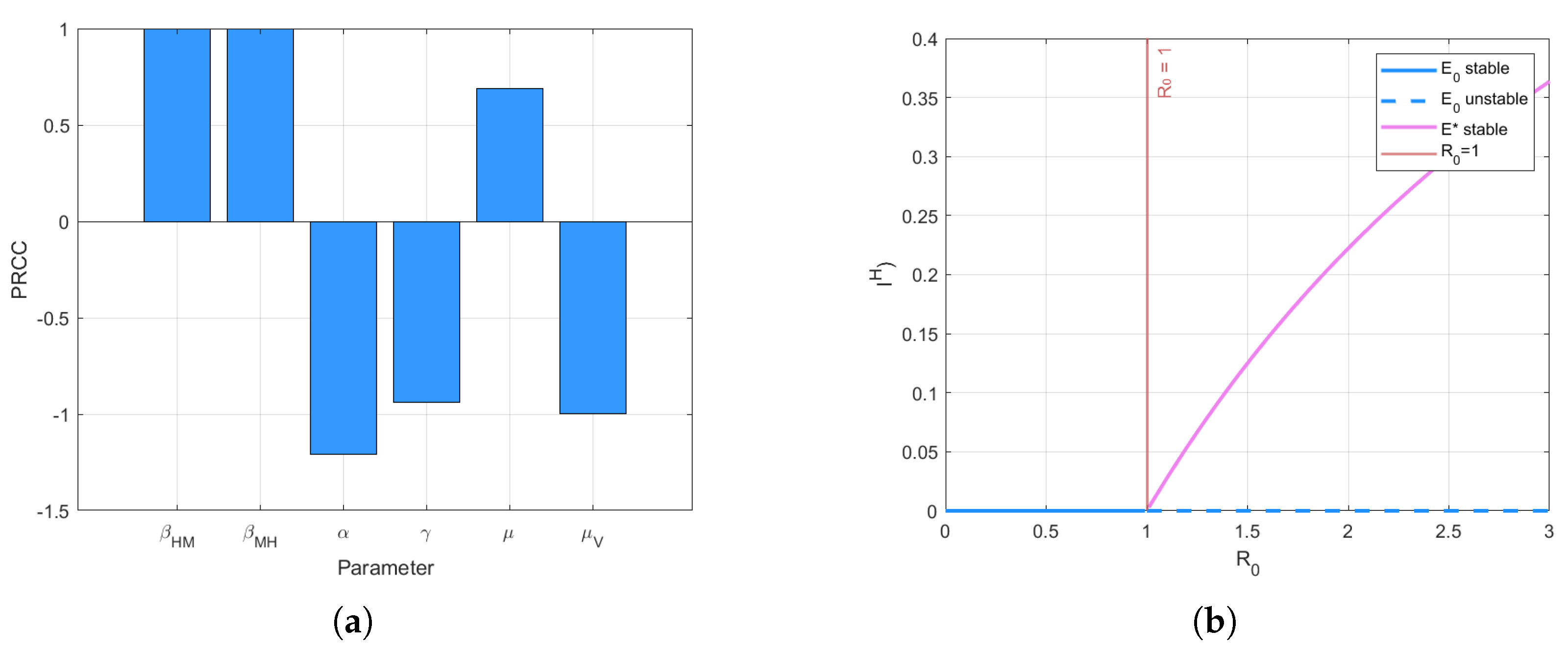
In Figure 2a, the sensitivity of R 0 to the parameters β ˜ , Λ , γ ˜ , and μ is calculated as follows:
A β M H = R 0 β M H β M H R 0 = 1 , A β H M = R 0 β H M β H M R 0 = 1 ,
A γ = R 0 γ γ R 0 = γ μ α γ μ α + μ , A μ ˜ = R 0 μ ˜ μ ˜ R 0 = 1 .
where A β ˜ , A Λ , A γ ˜ , and A μ represent the normalized sensitivity on β ˜ , Λ , γ ˜ , and μ , respectively. It is worth noting that the n times’ increase on β ˜ and Λ leads to the n times’ increase on R 0 , but the n times’ increase on γ ˜ and μ leads to the n times’ decrease on R 0 .
Then, the stability ranges of the disease-free equilibrium point E 0 and the endemic equilibrium point E * with respect to the basic reproduction number are given, as shown in Figure 2b.
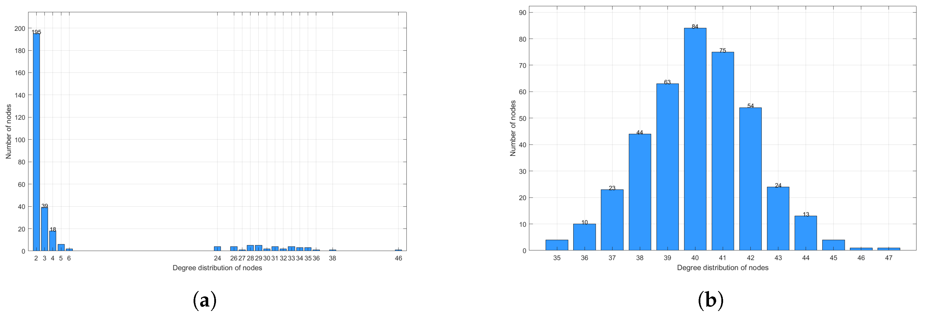
For the BA network, we have 300 nodes. While for the WS network, we have 400 nodes. The degree distribution is shown in Figure 3.
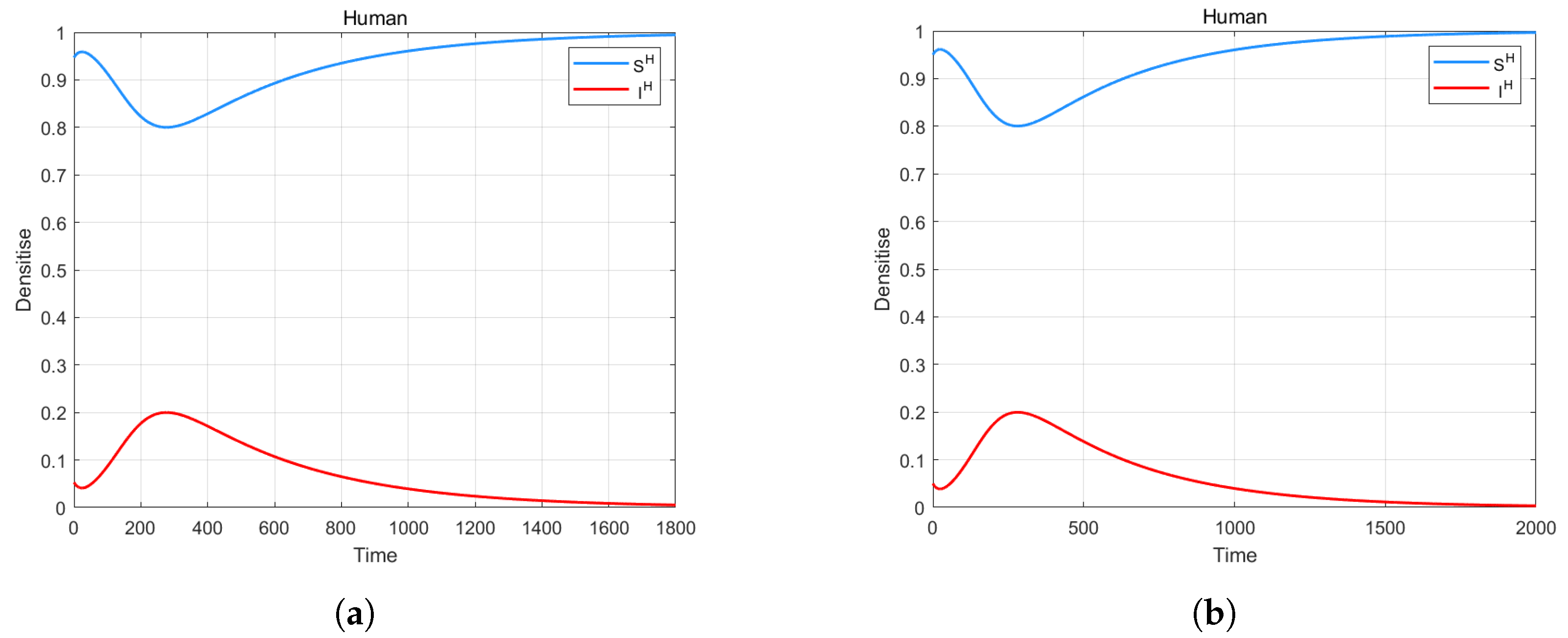
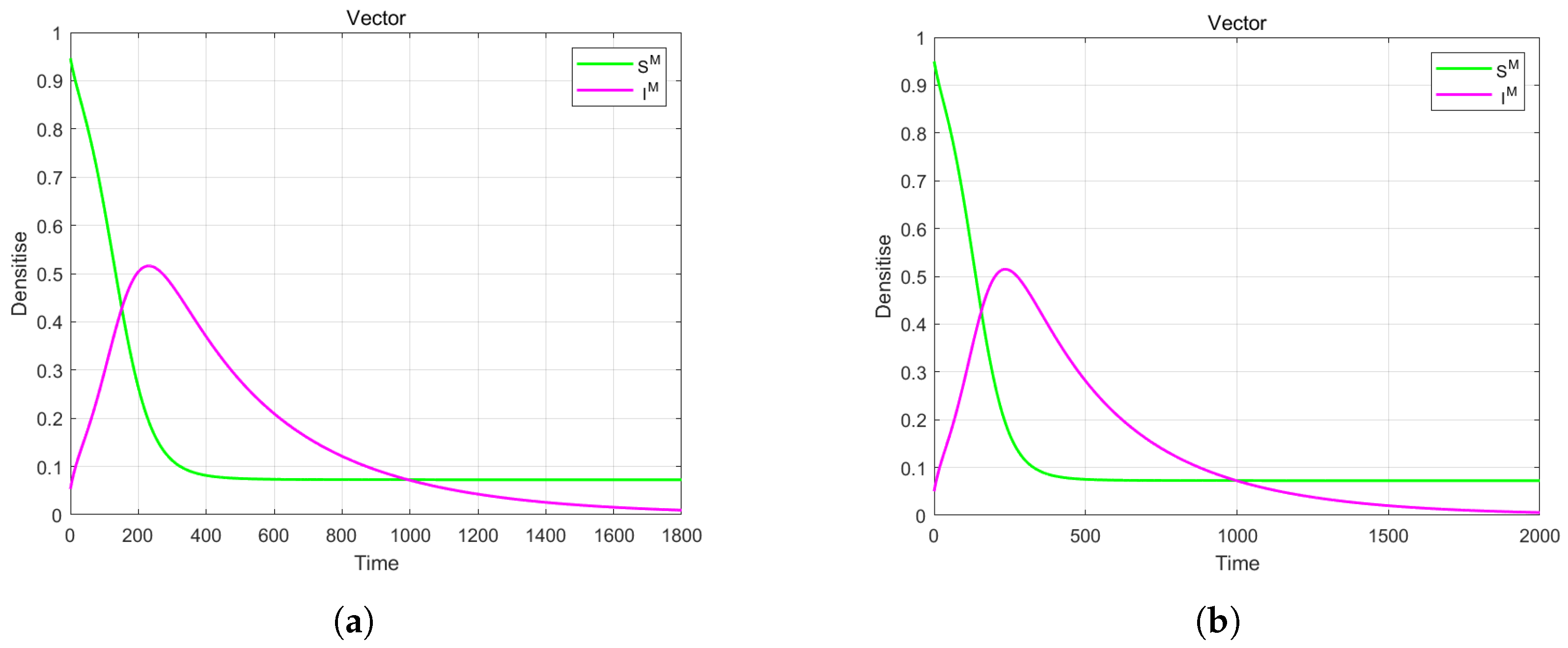
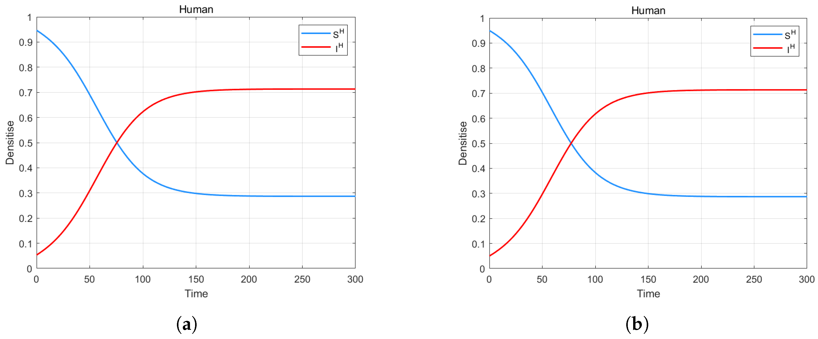
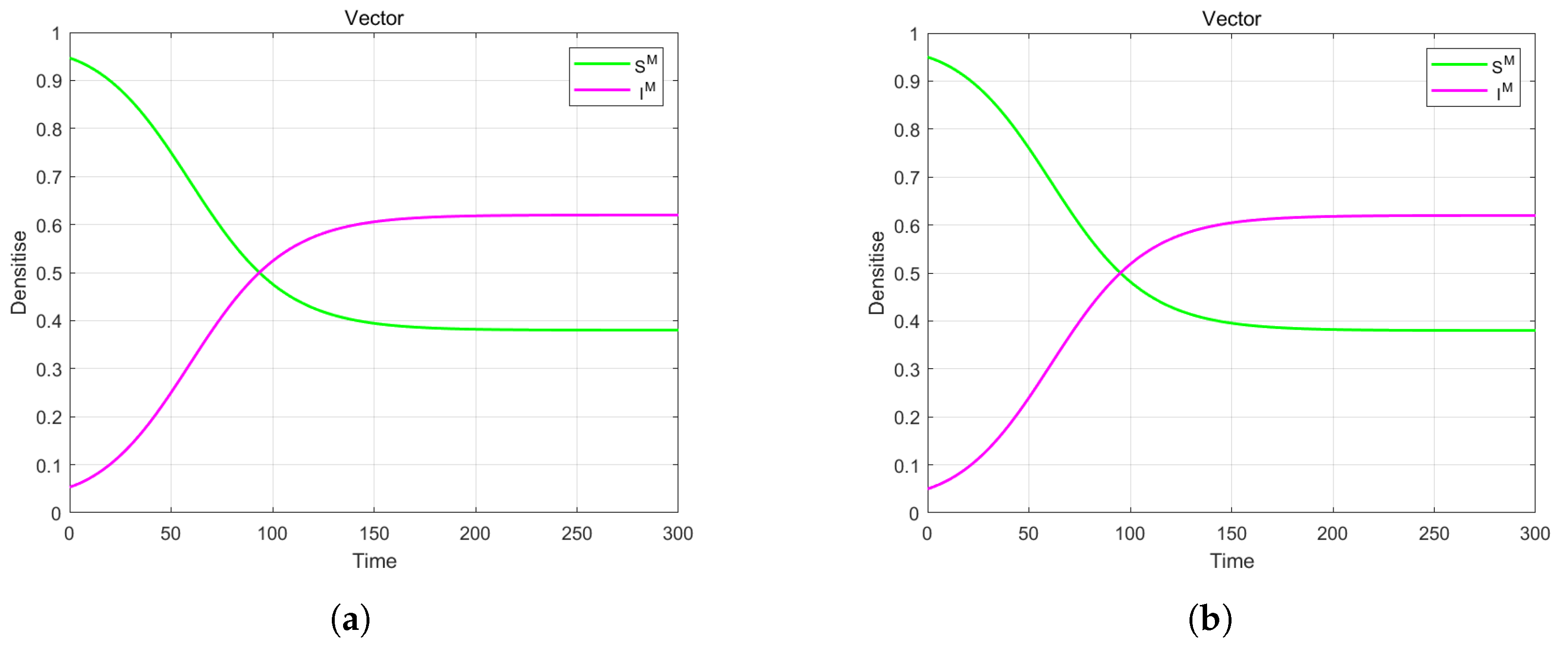
Let us suppose that α = 0.8 , β H M = 0.1 , β M H = 0.8 , μ = 0.2 , μ ˜ = 0.058 , γ = 0.85 , such that R 0 < 1 . According to Theorem 3, the disease-free equilibrium point E 0 is globally asymptotic-stable under the condition R 0 < 1 . For BA networks, the changes in human density over time are shown in Figure 4a, and the changes in vector density over time are shown in Figure 5a. For WS networks, the changes in human density over time are shown in Figure 4b, and the changes in vector density over time are shown in Figure 5b. That is to say, vector-borne diseases can die out. The simulation results also verify the correctness of Theorem 3. Epidemiologically, this has clear practical value: the vector-borne disease will eventually die out regardless of initial human or vector infection levels, with limited outbreak duration and no lingering low-level transmission. For control, R 0 targeted measures such as reducing vector biting rates via insecticides or boosting host recovery with treatment can push R 0 below 1, lowering peak prevalence while completely stopping the epidemic and eliminating resurgence risk.
Next, according to Theorem 4, the endemic equilibrium point E * is considered under the condition R 0 > 1 . We choose parameters α = 0.8 , β H M = 0.5 , β M H = 0.8 , μ = 0.2 , μ ˜ = 0.2 , γ = 0.3 , such that R 0 > 1 . The endemic equilibrium point E * is globally asymptotic-stable. For BA networks, the changes in human density over time are shown in Figure 6a, and the changes in vector density over time are shown in Figure 7a. For WS networks, the changes in human density over time are shown in Figure 6b, and the changes in vector density over time are shown in Figure 7b. That is to say, vector-borne diseases can persist. The simulation results also verify the correctness of Theorem 4. Biologically, this yields tangible epidemiological insights: the disease will persist long-term in the population, with indefinitely extended outbreaks instead of natural termination, and settle into a steady state where peak prevalence stabilizes as new infections balance recoveries and deaths. Short-term control such as temporary vector reduction that only lowers peak prevalence without cutting R 0 below 1 fails to stop sustained transmission, which emphasizes that R 0 -targeted long-term strategies such as long-acting vaccines or permanent vector habitat management are essential to disrupt the steady state and eliminate the disease.
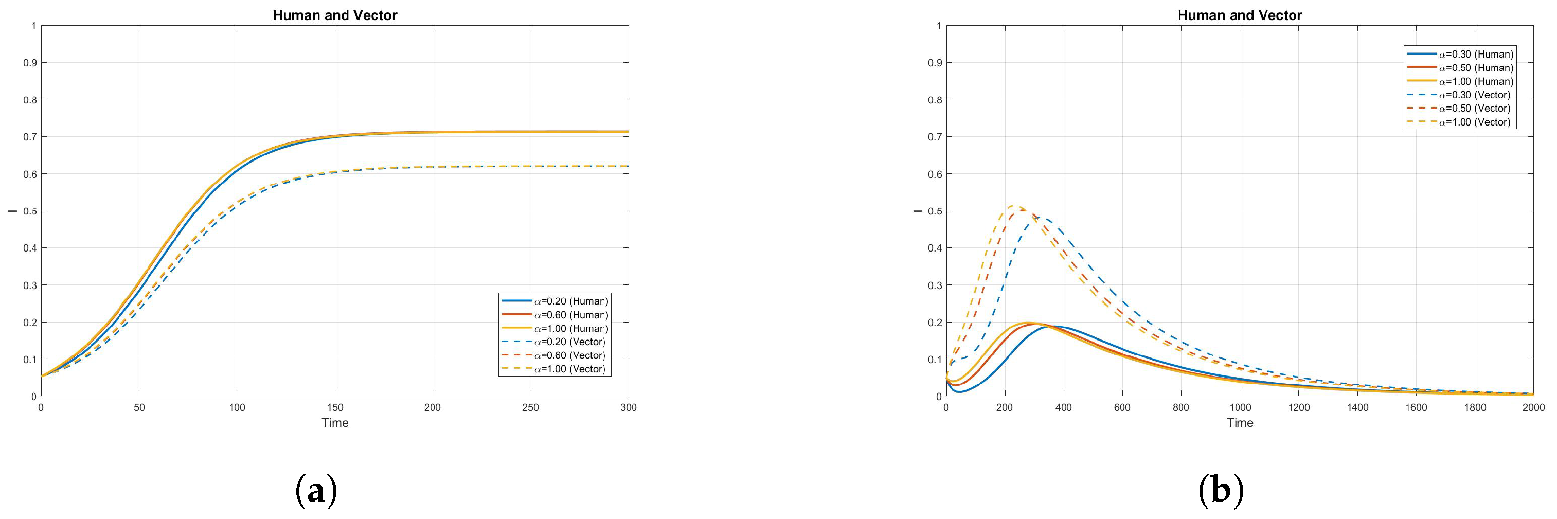
Then, we consider the analysis of the impact of variations of α on the behavior of the system and the stability of equilibria. For BA networks, we test different values of α , which are α = 0.2 , α = 0.6 , α = 1.0 and we use parameters β H M = 0.5 , β M H = 0.8 , μ = 0.2 , μ ˜ = 0.2 , γ = 0.3 . Figure 8a shows human density and vector density changes over time. For WS networks, we test different values of α , which are α = 0.3 , α = 0.5 , α = 1.0 and use parameters α = 0.8 , β H M = 0.1 , β M H = 0.8 , μ = 0.2 , μ ˜ = 0.058 , γ = 0.85 . Figure 8b shows human density and vector density changes over time. In essence, the equilibria peak represents the maximum accumulation of system states before stabilization. The peak difference between integer order ( α = 1 , no memory) and fractional-order ( 0 < α < 1 , with memory) models comes from memory’s regulation of the historical influence. Integer-order models have no historical constraints, so their state growth is more radical and leads to higher peaks. Fractional-order models are restricted by the attenuation of historical influence, so their growth is more gentle and peaks are always lower. To align with the real-world rule, fractional-order models are more meaningful for realistic predictions.

5. Conclusions

In this study, a fractional-order model for vector-borne diseases on bipartite networks is established. Human populations and vectors are considered as two distinct network layers. Meanwhile, the Riemann–Liouville (R-L) fractional integral is employed to describe the long-term memory behavior of infected populations during the recovery period. Subsequently, based on the condition for the unique existence of the endemic equilibrium point, the basic reproduction number associated with network topology and fractional order is derived. Furthermore, by analyzing the inherent properties of the model, conditions for the globally asymptotically stable disease-free equilibrium point and endemic equilibrium point of vector-borne infectious diseases are obtained. Finally, numerical simulation results on BA networks and WS networks are used to verify the theoretical conclusions of the model.

5.1. Limitations of the Proposed Approach

The proposed approach has some limitations. For network structure, it uses bipartite networks and respective human/vector average degrees to quantify transmission intensity, but not multilayer network analysis, which could integrate environmental, social, and genetic factors that affect real vector-borne disease spread. For rate assumptions, linear infection/recovery rates are adopted to clarify fractional-order models amid vector-borne diseases on bipartite networks. However, it lacks real-world nonlinear effects (saturation, herd immunity-driven risk reduction, behavior-based protection) that would improve alignment with actual epidemics.

5.2. Directions for Future Research

Future research directions will focus on three key aspects. First, method extensions: build on the current framework to integrate multilayer network structures—including environmental, social, and genetic factors as well as higher-order topology analyses—and nonlinear infection/recovery effects such as saturation and herd immunity impacts. Also, explore alternative fractional operators to compare their memory capture ability and clarify the suitability of the Riemann–Liouville operator. Second, empirical validation: address current data limitations by using real vector-borne disease datasets to calibrate model parameters, verify predictive reliability for outbreak duration and peak prevalence, and solve challenges from dynamic vector distributions, complex human behaviors, and incomplete public data. Third, application deepening: strengthen the link between theoretical results and public health practices, such as refining guidance for vaccination that prioritizes high human groups, medical resource allocation that focuses on regions with stronger memory effects, and vector control that targets reduction to make theoretical insights more actionable.

Author Contributions

Conceptualization, W.X. and Y.Y.; methodology, Z.L., C.W. and Y.Y.; software, C.W. and Y.H.; validation, W.X., Z.L. and Y.Y.; formal analysis, W.X.; investigation, W.X. and Y.Y.; writing—original draft preparation, W.X.; writing—review and editing, W.X., Y.Y. and Z.L.; visualization, C.W. and Z.L.; funding acquisition, W.X. and Y.Y. All authors have read and agreed to the published version of the manuscript.

Funding

This work is supported in part by the National Key R&D Program of China (2023YFC2605604) and the National Natural Science Foundation of China (Grant No. 62173027).

Data Availability Statement

Data are contained within the article.

Conflicts of Interest

The authors declare no conflicts of interest.

References

  1. Ross, R. The Prevention of Malaria; John Murray: London, UK, 1911. [Google Scholar]
  2. Wonham, M. The mathematics of mosquitoes and West Nile virus. Pi Sky 2004, 8, 5–9. [Google Scholar]
  3. Bergsman, L.D.; Hyman, J.M.; Manore, C.A. A mathematical model for the spread of West Nile virus in migratory and resident birds. Math. Biosci. Eng. 2016, 13, 401–424. [Google Scholar] [CrossRef] [PubMed]
  4. Eguda, A.J.; Yakubu, F. Analysis of a mathematical model to investigate the dynamics of dengue fever. J. Appl. Sci. Environ. Manag. 2017, 21, 626–638. [Google Scholar] [CrossRef]
  5. Qu, Z.; Xue, L.; Hyman, J.M. Modeling the transmission of Wolbachia in mosquitoes for controlling mosquito-borne diseases. SIAM J. Appl. Math. 2018, 78, 826–852. [Google Scholar] [CrossRef]
  6. Njoroge, K.P. Mathematical Modeling and Analysis of Transmission of Rift Valley Fever. Ph.D. Thesis, Kenyatta University, Nairobi, Kenya, 2019. [Google Scholar]
  7. Gebremeskel, A.A.; Krogstad, H.E. Mathematical modelling of endemic malaria transmission. Am. J. Appl. Math. 2015, 3, 36–46. [Google Scholar] [CrossRef]
  8. Masuda, N.; Konno, N. Multi-state epidemic processes on complex networks. J. Theor. Biol. 2006, 243, 64–75. [Google Scholar] [CrossRef]
  9. Bisanzio, D.; Bertolotti, L.; Tomassone, L.; Amore, G.; Ragagli, C.; Mannelli, A.; Giacobini, M.; Provero, P. Modeling the spread of vector-borne diseases on bipartite networks. PLoS ONE 2010, 5, e13796. [Google Scholar] [CrossRef]
  10. Zhang, R. Global dynamic analysis of a model for vector-borne diseases on bipartite networks. Phys. A Stat. Mech. Its Appl. 2020, 545, 123813. [Google Scholar] [CrossRef]
  11. Tanimoto, S. Epidemic spreading with immunization on bipartite networks. arXiv 2011, arXiv:1105.3265. [Google Scholar] [CrossRef]
  12. Hernandez, D.G.; Risau-Gusman, S. Epidemic thresholds for bipartite networks. Phys. Rev. E-Nonlinear Soft Matter Phys. 2013, 88, 052801. [Google Scholar] [CrossRef]
  13. Zhang, R.; Li, D.; Jin, Z. Dynamic analysis of a delayed model for vector-borne diseases on bipartite networks. Appl. Math. Comput. 2015, 263, 342–352. [Google Scholar] [CrossRef]
  14. Zhao, R.; Liu, Q.; Zhang, H. Dynamical behaviors of a vector-borne diseases model with two time delays on bipartite networks. Math. Biosci. Eng. 2021, 18, 3073–3091. [Google Scholar] [CrossRef] [PubMed]
  15. Latha, V.P.; Rihan, F.A.; Rakkiyappan, R.; Velmurugan, G. A fractional-order model for Ebola virus infection with delayed immune response on heterogeneous complex networks. J. Comput. Appl. Math. 2018, 339, 134–146. [Google Scholar] [CrossRef]
  16. Yusuf, A.; Acay, B.; Mustapha, U.T.; Inc, M.; Baleanu, D. Mathematical modeling of pine wilt disease with Caputo fractional operator. Chaos Solitons Fractals 2021, 143, 110569. [Google Scholar] [CrossRef]
  17. Muhammad, G.; Akram, M. Fuzzy fractional epidemiological model for Middle East respiratory syndrome coronavirus on complex heterogeneous network using Caputo derivative. Inf. Sci. 2024, 659, 120046. [Google Scholar] [CrossRef]
  18. Zhou, J.C.; Salahshour, S.; Ahmadian, A.; Senu, N. Modeling the dynamics of COVID-19 using fractal-fractional operator with a case study. Results Phys. 2022, 33, 105103. [Google Scholar] [CrossRef]
  19. Angstmann, C.N.; Henry, B.I.; McGann, A.V. A fractional-order infectivity SIR model. Phys. A 2016, 452, 86–93. [Google Scholar] [CrossRef]
  20. Angstmann, C.N.; Henry, B.I.; McGann, A.V. A fractional order recovery SIR model from a stochastic process. Bull. Math. Biol. 2016, 78, 468–499. [Google Scholar] [CrossRef]
  21. Angstmann, C.N.; Henry, B.I.; McGann, A.V. A general framework for fractional order compartment models. SIAM Rev. 2021, 63, 375–392. [Google Scholar] [CrossRef]
  22. Hirsch, W.M.; Herman, H.; Jean, P.G. Differential equation models of some parasitic infections: Methods for the study of asymptotic behavior. Commun. Pure Appl. Math. 1985, 38, 733–753. [Google Scholar] [CrossRef]
  23. Hirsch, M.W.; Smale, S.; Devaney, R.L. Differential Equations, Dynamical Systems, and an Introduction to Chaos; Academic Press: San Diego, CA, USA, 2013. [Google Scholar]
  24. Li, M.Y.; Muldowney, J.S. A geometric approach to global-stability problems. SIAM J. Math. Anal. 1996, 27, 1070–1083. [Google Scholar] [CrossRef]
  25. Li, M.Y.; Wang, L. Global Stability in Some SEIR Epidemic Models. In Mathematical Approaches for Emerging and Reemerging Infectious Diseases: Models, Methods, and Theory; Castillo-Chavez, C., Blower, S., Driessche, P., Kirschner, D., Yakubu, A., Eds.; Springer: New York, NY, USA, 2002; pp. 295–311. [Google Scholar]
  26. Gandica, Y.; Carvalho, J.; Aidos, F.S.D.; Lambiotte, R.; Carletti, T. Stationarity of the inter-event power-law distributions. PLoS ONE 2017, 12, e0174509. [Google Scholar] [CrossRef]
  27. Gandica, Y.; Carvalho, J. The origin of bursts and heavy tails in human dynamics. J. Phys. A Math. Theor. 2005, 38, 207–211. [Google Scholar]
  28. Vazquez, A.; Balazs, R.; Andras, L.; Barabasi, A. Impact of non-Poissonian activity patterns on spreading processes. Phys. Rev. Lett. 2007, 98, 158702. [Google Scholar] [CrossRef] [PubMed]
  29. Jo, H.H.; Moon, E.; Kaski, K. Optimized reduction of uncertainty in bursty human dynamics. Phys. Rev. E-Nonlinear Soft Matter Phys. 2012, 85, 016102. [Google Scholar] [CrossRef] [PubMed]
  30. Oliveira, J.G.; Barabási, A.L. Darwin and Einstein correspondence patterns. Nature 2005, 437, 1251. [Google Scholar] [CrossRef]
  31. Gonçalves, B.; Ramasco, J.J. Human dynamics revealed through Web analytics. Phys. Rev. E-Nonlinear Soft Matter Phys. 2008, 78, 026123. [Google Scholar] [CrossRef]
  32. Candia, J.; González, M.C.; Wang, P.; Schoenharl, T.; Madey, G.; Barabási, A.-L. Uncovering individual and collective human dynamics from mobile phone records. J. Phys. A Math. Theor. 2008, 41, 224015. [Google Scholar] [CrossRef]
  33. Radicchi, F. Human activity in the web. Phys. Rev. E-Nonlinear Soft Matter Phys. 2009, 80, 026118. [Google Scholar] [CrossRef]
  34. Chaintreau, A.; Hui, P.; Crowcroft, J.; Diot, C.; Gass, R.; Scott, J. Impact of human mobility on opportunistic forwarding algorithms. IEEE Trans. Mob. Comput. 2006, 6, 620. [Google Scholar]
  35. Freedman, H.L.; Ruan, S.; Tang, M. Uniform persistence and flows near a closed positively invariant set. J. Dyn. Differ. Equ. 1994, 6, 583–600. [Google Scholar] [CrossRef]
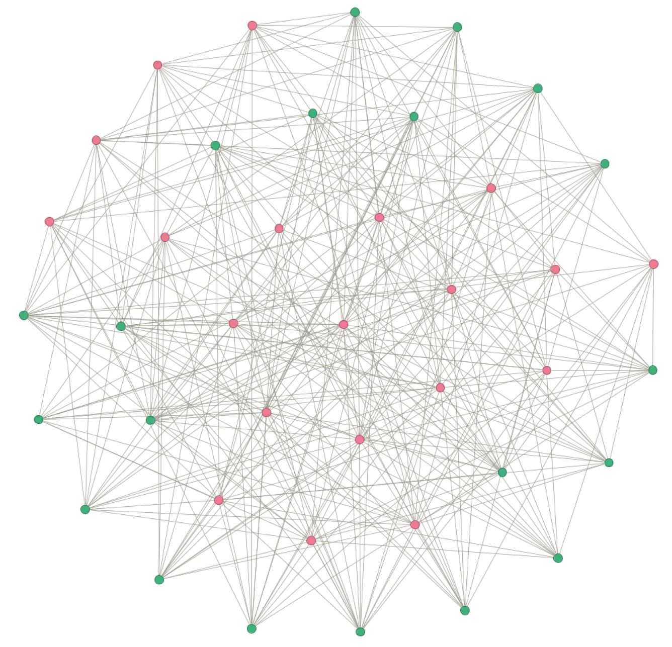
Figure 1. The structure of a bipartite network: the red nodes represent human, and the green nodes represent vector.
Fractalfract 09 00742 g001
Figure 2. Property of R 0 ; (a) sensitivity analysis; (b) stability region.
Fractalfract 09 00742 g002
Figure 3. The degree distribution of the networks; (a) BA network; (b) WS network.
Fractalfract 09 00742 g003
Figure 4. The disease-free equilibrium point of the networks; (a) BA network; (b) WS network.
Fractalfract 09 00742 g004
Figure 5. The disease-free equilibrium point of the networks; (a) BA network; (b) WS network.
Fractalfract 09 00742 g005
Figure 6. The endemic equilibrium point of the networks; (a) BA network; (b) WS network.
Fractalfract 09 00742 g006
Figure 7. The endemic equilibrium point of the networks; (a) BA network; (b) WS network.
Fractalfract 09 00742 g007
Figure 8. The impact of the different α ; (a) BA network; (b) WS network.
Fractalfract 09 00742 g008
Disclaimer/Publisher’s Note: The statements, opinions and data contained in all publications are solely those of the individual author(s) and contributor(s) and not of MDPI and/or the editor(s). MDPI and/or the editor(s) disclaim responsibility for any injury to people or property resulting from any ideas, methods, instructions or products referred to in the content.